HAL Id: halshs-00586834https://halshs.archives-ouvertes.fr/halshs-00586834

Preprint submitted on 18 Apr 2011

HAL is a multi-disciplinary open accessarchive for the deposit and dissemination of sci-entific research documents, whether they are pub-lished or not. The documents may come fromteaching and research institutions in France orabroad, or from public or private research centers.

L’archive ouverte pluridisciplinaire HAL, estdestinée au dépôt et à la diffusion de documentsscientifiques de niveau recherche, publiés ou non,émanant des établissements d’enseignement et derecherche français ou étrangers, des laboratoirespublics ou privés.

European integration, FDI and the geography of Frenchtrade

Miren Lafourcade, Elisenda Paluzie

To cite this version:Miren Lafourcade, Elisenda Paluzie. European integration, FDI and the geography of French trade.2008. �halshs-00586834�

WORKING PAPER N° 2008 - 13

European integration, FDI and the geography of French trade

Miren Lafourcade

Elisenda Paluzie

JEL Codes: F15, F23, R12, R58 Keywords: trade, gravity, border regions, European

integration, foreign direct investment

PARIS-JOURDAN SCIENCES ECONOMIQUES

LABORATOIRE D’ECONOMIE APPLIQUÉE - INRA

48, BD JOURDAN – E.N.S. – 75014 PARIS TÉL. : 33(0) 1 43 13 63 00 – FAX : 33 (0) 1 43 13 63 10

www.pse.ens.fr

CENTRE NATIONAL DE LA RECHERCHE SCIENTIFIQUE – ÉCOLE DES HAUTES ÉTUDES EN SCIENCES SOCIALES ÉCOLE NATIONALE DES PONTS ET CHAUSSÉES – ÉCOLE NORMALE SUPÉRIEURE

European Integration, FDI and the Geography of French Trade∗

Miren Lafourcade† Elisenda Paluzie‡

March 27, 2008

Abstract

This paper uses an augmented gravity model to investigate whether the 1978-2000 process of

European integration has changed the geography of trade within France, with a particular focus

on the trends experienced by border regions. We support the conclusion that, once controlled for

bilateral distance, origin- and destination-specific characteristics, French border regions trade on

average 72% more with nearby countries than predicted by the gravity norm. They perform even

better (114%) if they have good cross-border transport connections to the neighboring country.

However, this outperformance eroded drastically for the French border regions located at the pe-

riphery of Europe throughout integration. We show that this trend is partly due to a decreasing

propensity of foreign affiliates to trade with their home country. This trade reorientation is less

pronounced for the Belgian-Luxembourgian and German firms located in the regions which have

better access to the EU core.

JEL classification: F15, F23, R12, R58.

Keywords: Trade, Gravity, Border regions, European Integration, Foreign Direct Investment.

∗This paper has been prepared as part of a PREDIT research contract (Grant No:04-MT-5036). We would like to

thank the French Ministry of Transport, specially Alain Sauvant and Micheline Travet, for providing us with French trade

data in return for financial contractual obligations and strict confidentiality. We also acknowledge the French Government

Agency For International Investment (and more particularly David Cousquer and Clotilde Lainard) and Thierry Mayer

for their kind help in gathering data. We are indebted to Anthony Briant, Melika Ben Salem, Pierre-Philippe Combes,

Joan Costa, Laurent Gobillon, Giordano Mion, Jordi Pons, Muriel Roger, Egle Tafenau and Daniel Tirado for insightful

suggestions. Conference participants in Glasgow (February 2005), Cagliari (May 2005), Kiel (June 2005), Barcelona

(July 2005) and Amsterdam (August 2005) provided us with fruitful comments. Financial supports from the CEPR

Research Network on The Economic Geography of Europe: Measurement, Testing and Policy Simulations, funded by the

European Commission under the Research Training Network Programme (Contract No: HPRN-CT-2000-00069), from

the Spanish Ministry of Science and Technology (Project SEC2002-03212), the Spanish Ministry of Education (Project

SEJ2005-03196/ECON) and the Catalan Government (2005SGR-00460) are also gratefully acknowledged.†Corresponding author. University of Valenciennes and Paris School of Economics (PSE). PSE, 48 Bd. Jourdan,

75014 Paris, France. lafourcade@pse.ens.fr. http://www.enpc.fr/ceras/lafourcade/.‡Universitat de Barcelona (Departament de Teoria Economica, CAEPS). epaluzie@ub.edu

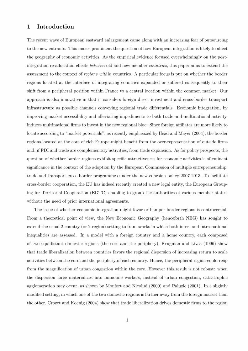
1 Introduction

The recent wave of European eastward enlargement came along with an increasing fear of outsourcing

to the new entrants. This makes prominent the question of how European integration is likely to affect

the geography of economic activities. As the empirical evidence focused overwhelmingly on the post-

integration re-allocation effects between old and new member countries, this paper aims to extend the

assessment to the context of regions within countries. A particular focus is put on whether the border

regions located at the interface of integrating countries expanded or suffered consequently to their

shift from a peripheral position within France to a central location within the common market. Our

approach is also innovative in that it considers foreign direct investment and cross-border transport

infrastructure as possible channels conveying regional trade differentials. Economic integration, by

improving market accessibility and alleviating impediments to both trade and multinational activity,

induces multinational firms to invest in the new regional bloc. Since foreign affiliates are more likely to

locate according to “market potentials”, as recently emphasized by Head and Mayer (2004), the border

regions located at the core of rich Europe might benefit from the over-representation of outside firms

and, if FDI and trade are complementary activities, from trade expansion. As for policy prospects, the

question of whether border regions exhibit specific attractiveness for economic activities is of eminent

significance in the context of the adoption by the European Commission of multiple entrepreneurship,

trade and transport cross-border programmes under the new cohesion policy 2007-2013. To facilitate

cross-border cooperation, the EU has indeed recently created a new legal entity, the European Group-

ing for Territorial Cooperation (EGTC) enabling to group the authorities of various member states,

without the need of prior international agreements.

The issue of whether economic integration might favor or hamper border regions is controversial.

From a theoretical point of view, the New Economic Geography (henceforth NEG) has sought to

extend the usual 2-country (or 2-region) setting to frameworks in which both inter- and intra-national

inequalities are assessed. In a model with a foreign country and a home country, each composed

of two equidistant domestic regions (the core and the periphery), Krugman and Livas (1996) show

that trade liberalization between countries favors the regional dispersion of increasing return to scale

activities between the core and the periphery of each country. Hence, the peripheral region could reap

from the magnification of urban congestion within the core. However this result is not robust: when

the dispersion force materializes into immobile workers, instead of urban congestion, catastrophic

agglomeration may occur, as shown by Monfort and Nicolini (2000) and Paluzie (2001). In a slightly

modified setting, in which one of the two domestic regions is farther away from the foreign market than

the other, Crozet and Koenig (2004) show that trade liberalization drives domestic firms to the region

1

closer to the border, unless competition pressure from the foreign market is too fierce. As opening

up to trade with a foreign economy increases exports (foreign demand) and imports (foreign supply),

the impact of trade liberalization is the result of two counteracting forces: increased market access

(favorable to export production) and increased import competition (negative for domestic producers

that compete with foreign supply).

Nonetheless, the core-periphery models of the Krugman’s type are not only known for the extreme

result that trade costs reduction would yield catastrophic agglomeration, but also for their analytical

intractability. Hence, recent studies have tried both to attenuate centripetal forces and to provide

analytical solutions to the models. For instance, Brulhart et al. (2004) build a 3-region setting in which

the manufacturing sector uses mobile human capital as the fixed cost and immobile workers as the

variable cost of production. They find that, for most parameter configurations, trade liberalization

favors the concentration of human capital in the border region. However, this mechanism is not

deterministic: A sufficiently strong pre-liberalization concentration of economic activity in the interior

region can make this concentration globally stable, and predicts even more agglomeration in this

region. Behrens et al. (in press) develop a 2-country 4-region model in which low inter-country

trade costs is shown to promote regional dispersion when inter-regional trade costs are high enough.

Behrens et al. (2006) use the same model to investigate the role of “gate” regions, through which

goods are shipped to the international market. If one country is endowed with such a region, the latter

benefits from agglomeration when the country is well integrated whereas, in the other case, it is the

landlocked region. Therefore, theory has not reached a consensus on whether or not border regions

might benefit from integration processes. Hence, empirical analysis is even more crucial to identify

the main mechanisms at work.

The main empirical approach consists in testing the NEG predictions of backward (demand)

linkage effects:1 the better a region’s access to large markets, the higher its factor prices, output, or

a mix of the two. Therefore, regional wage gradients, which were initially decreasing monotonously

from center to periphery, might possibly reverse consequently to changes in trade regimes and market

potentials. As for output variables, adjustments are driven by the number of firms, and regions with

good access to foreign markets end up with a higher share of activities. Regarding North-America,

Hanson (1996a, 1996b, 1997, 2001) are among the pioneer empirical studies assessing whether the

NAFTA process entailed changes in wages or employment within participating countries. While they

provide strong evidence of jobs relocation by the two sides of the U.S.-Mexico border following NAFTA,

they do not yet support unequivocally the wage gradients reversal prediction. EU prospects concern

1See Niebuhr and Stiller (2004) for a comprehensive survey.

2

mostly the recent eastward enlargement and the fear that, as the borders of CEE countries become

internal to the EU, economic activities could shift towards Eastern border locations, eventually at

the expense of Western border regions. For instance, Brulhart and Koenig (2006) compare the wage

gradients of five accession countries (Czech Republic, Hungary, Poland, Slovenia and Slovakia) to

those of incumbent EU countries, for the period 1996-2000. They find that concentration in the capital

regions is significantly stronger in the former and that nominal wages are higher in the border regions

of incumbent EU countries. Hence, they conjecture that market forces would likely favor Eastern

border regions. Based on simulated changes in the market accessibility of EU27 regions, Niebuhr

(2005) also supports the conjecture that border regions could experience above-average integration

benefits due to their favorable access to foreign markets. A noticeable exception to the eastward focus

is the recent work by Overman and Winters (2003, 2005), who examine whether the UK’s accession to

the EEC in 1973 impacted the location of domestic manufacturing activities within the UK. Accession

is shown to have a mitigated effect: even though manufacturing activities might have relocated south-

eastwards, several industries also retreated north-westwards, because of increased import competition.

Therefore, the empirical estimation of backward linkages, both in the factor price version (wages) and

quantity version (employment or production) indicates that regions bordering the largest and richest

markets do seem to benefit from economic integration with them. By contrast, the results for regions

bordering poorer markets are more mixed. Some of them, like the South of the US, experience positive

effects while for others, particularly in Eastern Europe, the impact might be negative.

Our empirical approach is different in that first, we focus on the western part of Europe and

secondly, we concentrate on trade rather than on wage and employment issues. Post-integration

changes in trade performances that would depend on where regions are located within countries have

been rarely investigated. Two noticeable exceptions have to be mentioned. First, Coughlin and Wall

(2003) distill the trade impact of NAFTA on the US states. Their conclusion is that, following NAFTA,

28 (36, respectively) U.S. states experienced a rise of more than 10% in their exports towards Mexico

(Canada, respectively), while 8 (4, respectively) were negatively affected. However, the core-periphery

nature of winners and losers is not assessed. In contrast, Egger and Pfaffermayr (2002) analyze the

trade impact of the 1960-1998 process of EU integration, with a special focus on trade within and

between the core and periphery countries. They find out that, while both core-periphery and intra-

periphery countries benefited more from EU integration than intra-core countries, this positive effect

reduced throughout the enlargement. The southern enlargement even turned to exert a negative effect

on the intra-core volume of trade.

In line with Egger and Pfaffermayr (2002), we assess the trade differentials sparked by European

integration, but we focus on the case of French regions. We develop an augmented gravity model in

3

which European integration is materialized through the reduction of FDI barriers. We then quantify

the trade performance of border regions as their deviation from the value of trade predicted by this

gravity norm. We find evidence that, everything else equal, French border regions trade on average

72% more with nearby countries than predicted by the norm, and even more (114%) if they have

good cross-border transport connections. However, the process of European integration has coincided

with a large decrease in this trade overperformance over the period 1978-2000. This trend was driven

by the drastic fall in the deviations experienced by the most peripheral French border regions within

the EU. Neither the Single European Act nor the completion of the Single Market were sufficient

to counterbalance the decline. We find that these trade differentials can partly be attributed to

FDI regional patterns, and more precisely to a decreasing scope for trading with the home country.

However, this trend is less pronounced for the Belgian-Luxembourgian and German firms located at

the vicinity of the EU core.

The remainder of the paper proceeds as follows. Section 2 provides some stylized evidence on the

suitability of the gravity framework for the study of the interplay between trade performances and

FDI. Section 3 describes the augmented gravity model, as well as the data and methodological issues.

Section 4 provides two sets of results for France. The first set relates to the 1978-2000 long-span

evolution of trade differentials between border and interior regions, whereas the second set analyzes

more specifically the role of inward FDI in the period 1993-2000. Section 5 concludes.

2 Trade and FDI patterns of French regions: Stylized evidence

A detailed assessment on whether integration is likely to affect the internal geography of trade requires

a thorough theoretical and econometric analysis, that we will seek to provide in subsequent sections.

However, if border regions experience specific trends arising from the counteracting forces described in

the Introduction, we should be able to pick up them with the naked eye. Section 2 therefore provides

a set of stylized facts on the trade and FDI patterns of French regions.

2.1 Trade specialization patterns by country

To illustrate that proximity is a clear catalyst for trade, a brief look at the relative trade performances

of regions inside France is instructive.2 So as to assess the relative specialization of regions across

partner countries, we compute the following trade index. Let J denote the trade partner country of

2As we seek for trade differentials depending on whether regions border a country or not, we examine only the sixEU countries neighboring France: Belgium, Luxembourg, Germany, United-Kingdom, Spain and Italy. Due to dataconstraints, we treat Belgium and Luxembourg as a single partner country for French regions. Appendix A presents thedata sources.

4

region i. We define siJ = FiJ/∑

i∈I FiJ as the share of region i in the country I’s trade with country

J , and xi =∑

K FiK/∑

i∈I

∑K FiK as its share in the country I’s international trade. The simplest

way to measure how much the trade of region i is oriented towards the partner country J , and to

compare this trade intensity across countries, is to compute the following Balassa Trade Specialization

Index:

TSIiJ =siJ

xi× 100. (1)

Values above 100 mean that region i trades relatively more with country J than would be predicted

by its share in international trade. Figures 1 and 2 exhibit the patterns obtained in 2000.

Figure 1: Trade specialization of French regions with respect to: Spain (top) and Italy (bottom)

Source: Authors’ computations based on data from the SITRAM database (French Ministry of Transport). See Appendix A for further details.

The gravity pattern of trade is striking: regardless of the direction of trade, border regions always

outperform “vis-a-vis” the countries with which they share a frontier. This pattern is especially clear at

the French borders with Belgium-Luxembourg and Germany. For instance, with a TSI of respectively

280 for exports and 355 for imports, the French NUTS3 “Ardennes”, which borders Belgium, is almost

four times more export-oriented towards this country than with the rest of the world.

5

Hence, proximity gives the agents located on both sides of the same frontier clear incentives to

trade. Sometimes however, specific border regions have a surprisingly low TSI. For instance, in the

NUTS3 region of “Haute-Garonne”, which hosts Toulouse and has a border with Spain, mountains in

the central part of the Pyrenees represent a major geographic obstacle and make cross-border transport

particularly difficult. Therefore, a strict contiguity criterion is not always sufficient to embody the real

border nature of regions, as the geography of frontiers may also deeply affect trade specializations.

Furthermore, interior regions sometimes present surprisingly high levels of specialization with

regard to a partner country, in spite of being located very far away. One first plausible explanation is

that cross-border input-output linkages might generate specific patterns which are not necessarily of

the gravity type. For instance, the French central regions of “Puy de Dome” and “Vienne” exhibit a

strong specialization of exports oriented towards Germany, probably due to the presence of the French

firm Michelin, which produces equipment goods for German firms such as BMW, Daimler-Chrysler and

Volkswagen A.G. A second explanation is that vertical outsourcing, which enables foreign investors

to benefit from advantages other than reduced transport costs (such as low taxes, rents or wages)

might also cause extreme specialization patterns. Foreign inward direct investment from neighboring

countries is likely to boost trade due to input-output linkages between the foreign parent firm in the

home country and its affiliates in the host region. For instance, the south region of “Haute-Garonne”

comes out as the most specialized regarding exports to Germany, although it is located on the opposite

side of this country. The reason may be that it hosts the European Aeronautic Defence and Space

(EADS) consortium, of which the German firm Daimler-Chrysler owns more than 30%. Therefore, to

compare the trade performance and orientation of regions we have to bear in mind that FDI might

expand the trade of interior as well as of border regions. Next section focuses more specifically on

this issue.

2.2 FDI specialization patterns by country

Figure 3 depicts the inward stocks of Foreign inward Direct Investment based on four different vari-

ables: Number of foreign affiliates, created or saved related employment (hence, zero indicates green-

field investment), and millions of euros invested.3

3Appendix A presents the data sources.

6

Figure 2: Trade specialization of French regions with respect to: United-Kingdom (top), Belgium-Luxembourg (middle) and Germany (bottom)

Source: Authors’ computations based on data from the SITRAM database (French Ministry of Transport). See Appendix A for further details.

7

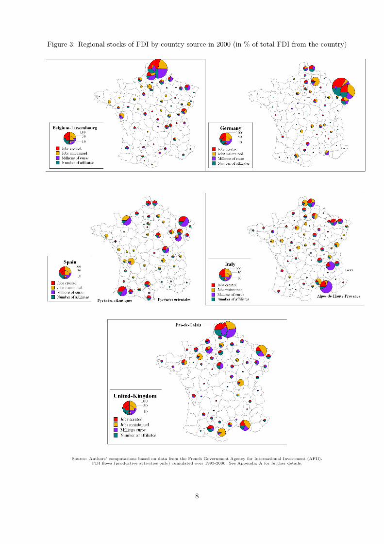
Figure 3: Regional stocks of FDI by country source in 2000 (in % of total FDI from the country)

Source: Authors’ computations based on data from the French Government Agency for International Investment (AFII).FDI flows (productive activities only) cumulated over 1993-2000. See Appendix A for further details.

8

Two striking features arise from this picture. First, regardless of their nationality, foreign firms

have a clear preference for the regions located along the north-eastern frontier of France. These border

regions present conducive conditions for investment as they benefit from good access to the richest

internal French regions, due to the high density of highway infrastructures towards the French capital,4

and also to the core of Europe. As the propensity to invest increases with market potentials (Head and

Mayer, 2004), the north-eastern French border represents a good trade-off between the desire to save

on accessing French consumers and the costs of operating in rich European markets at the same time.

Secondly, foreign firms also target the regions located at the other side of their home frontier, which

may feed their trade expansion. As argued in Crozet et al. (2004), the similarity in cultures around

the two sides of a same frontier is likely to distort FDI patterns at the benefit of the regions nearby

home country. Gravity forces may even extend beyond such regions due to the spatial propagation of

preferences. Other features such as natural geographic impediments may also increase the propensity

of foreign firms to target some of the border regions at the expense of others, or to locate a bit further

away from the border. Hence, Italian firms favor the “Isere” region at the expense of the mountainous

“Alpes-de-Haute-Provence”, whereas Spanish firms clearly prefer to locate in “Pyrenees atlantiques”

and “Pyrenees orientales”, where smoother relief allows for pass-roads. The same trend is very salient

for British firms, who prefer to locate in “Pas-de-Calais” region, which benefits from the Euro-tunnel

connection to the UK. These features stress the heterogeneity of border regions, and the need to

qualify their border nature according to the geography of frontiers.

Finally, it is worth noting that exceptions to these two trends, which are found in some regions,

confirm some of the conjectures given in section 2.1. For instance, despite its remoteness, the south-

central region of “Aveyron”, whose exports are strongly oriented towards Germany, hosts a large share

of the total German FDI.5

3 Trade specifications, data and econometric issues

Section 3 presents the theoretical mechanisms underpinning the interplay between economic integra-

tion, multinational activity and trade (Section 3.1), and provides some clue on the data and estimation

issues (Section 3.2).

4See Combes and Lafourcade (2005) for a more detailed picture of the relative transport accessibility of French regions.5As is well known, Bosch is one of the German affiliates located in this region.

9

3.1 The augmented gravity model

The representative utility in region i depends on the consumption of the nJt varieties produced in each

foreign partner country J , ciJt.6 Varieties are differentiated with a constant elasticity of substitution

(CES). Goods being heterogeneous across countries, we use the Armington’s (1969) assumption that

consumers might prefer the varieties produced in some countries at the expense of others: parameter

aiJt captures the preference bias of consumers in region i with respect to the varieties produced in J .

The utility function in region i is:

Uit =

(∑

J

∑nJt

(aiJtciJt)σ−1

σ

) σσ−1

, (2)

where σ > 1 is the elasticity of substitution between the varieties produced abroad.

Let piJt denote the delivered price in region i of any variety produced in country J , τiJt, the ad

valorem trade cost, and pJt the mill price in J . We have piJt = (1 + τiJt) pJt.

It is straightforward to obtain the following expression for imports originating from J :

ciJt = citPσ−1it nJtp

1−σJt aσ−1

iJt (1 + τiJt)1−σ , (3)

where cit =∑

J

∑h ciJht is total demand in region i for varieties originating from all foreign sources,

and Pit, the price index in region i, Pit ≡(∑

J aσ−1iJt nJtp

1−σiJt

)1/(1−σ).

We assume that trade costs are composed of two different elements: transport costs, TiJt, and

specific cross-border costs, BiJt:

(1 + τiJt)σ−1 = TiJtBiJt. (4)

Transport costs have the following symmetric structure:

TiJt = TJit = (distiJ)δ exp(1− βT

1 bord1iJ − βT2 bord2iJ

), (5)

where bord1iJ and bord2iJ are contiguity dummies capturing the border nature of regions. bord1iJ = 1

indicates that the NUTS3 region i shares a frontier with country J (first-order contiguity criterion),

while bord2iJ = 1 means that, absent strict contiguity, the NUTS3 region i belongs to a NUTS2

region that shares a frontier with country J (second-order contiguity criterion). Moreover, if, absent

transport gateways, trade cannot transit through the border of region i to accede market J (due for

6In the rest of the paper, small letters will refer to regions and capital letters to countries. The subscript t indicatesthat the variable is time-variant.

10

instance to mountains), the two previous dummies are set to 0, which means that region i is treated

as interior and not border. Therefore, we capture the “real” border nature of regions by taking into

account their endowments in cross-border infrastructures in addition to their location at the political

frontier. As cross-border transport connections alleviate the cost of shipping goods through the border,

parameters βT1 and βT

2 are both expected to be positive. Finally, more standardly, transport costs

increase with the distance incurred to ship goods between region i and country J , distiJ .

Specific cross-border costs, BiJt, include first tariffs tIJt. The protection structure depends only

on bilateral trade agreements signed by countries I and J , which are uniform across border and non-

border regions. Advances in European integration are reflected in the progressive removal of tariffs,

but also in the alleviation of informal barriers to trade, denoted ntbiJt, that might affect either border

or non-border regions differently. We assume:

BiJt = (1 + tIJt)(1 + ntbiJt) = (1 + fdiiJt)−αB, (6)

where fdiiJt is a measure of the inward stock of bilateral foreign direct investment.7

The relationship between trade barriers and FDI is a rather disputed issue in theory (Neary, 2002;

Faini, 2004). Consequently, there is no clear assertion on the question whether multinational activity

and trade should be complements or substitutes.8 On one side, the reduction in trade barriers alleviates

the costs for foreign firms of operating outside their home market, which should give multinationals

more incentives to fragment production. If region i benefits from lower input costs relatively to other

regions, it should be targeted for vertical outsourcing. If foreign affiliates trade back and forth with

parent firms located in the home country, there should be a positive causation between FDI and both

the imports and exports of the recipient region. Moreover, a number of recent models explain the

propensity of more productive firms to self-select into multinational activity.9 This could generate an

additional trade-expanding effect for the recipient regions. A huge body of empirical literature actually

supports the evidence that multinational activity and trade would be complementary activities (Lipsey

and Weiss, 1981, 1984; Pfaffermayr, 1996; Clausing, 2000; Head and Ries, 2001). However, on the other

side, standard theory of multinational corporation predicts a proximity-concentration trade-off which

leads firms to outsource production when trade barriers are large and scale economies at the plant

level outpace scale economies at the industry level (Brainard, 1997). Therefore, horizontally-motivated

7The direction of FDI is therefore assumed to be the same as imports. A proper modeling of border barriers wouldrequire the addition of the outward stock, fdiJit, which would entail more plausible asymmetric trade costs. However,absent data, we have to restrict to inward FDI only.

8Forte (2004) provides an exhaustive survey of both the theoretical and empirical literatures on this question.9See among others Bernard et al. (2003), Melitz (2003), Helpman et al. (2004).

11

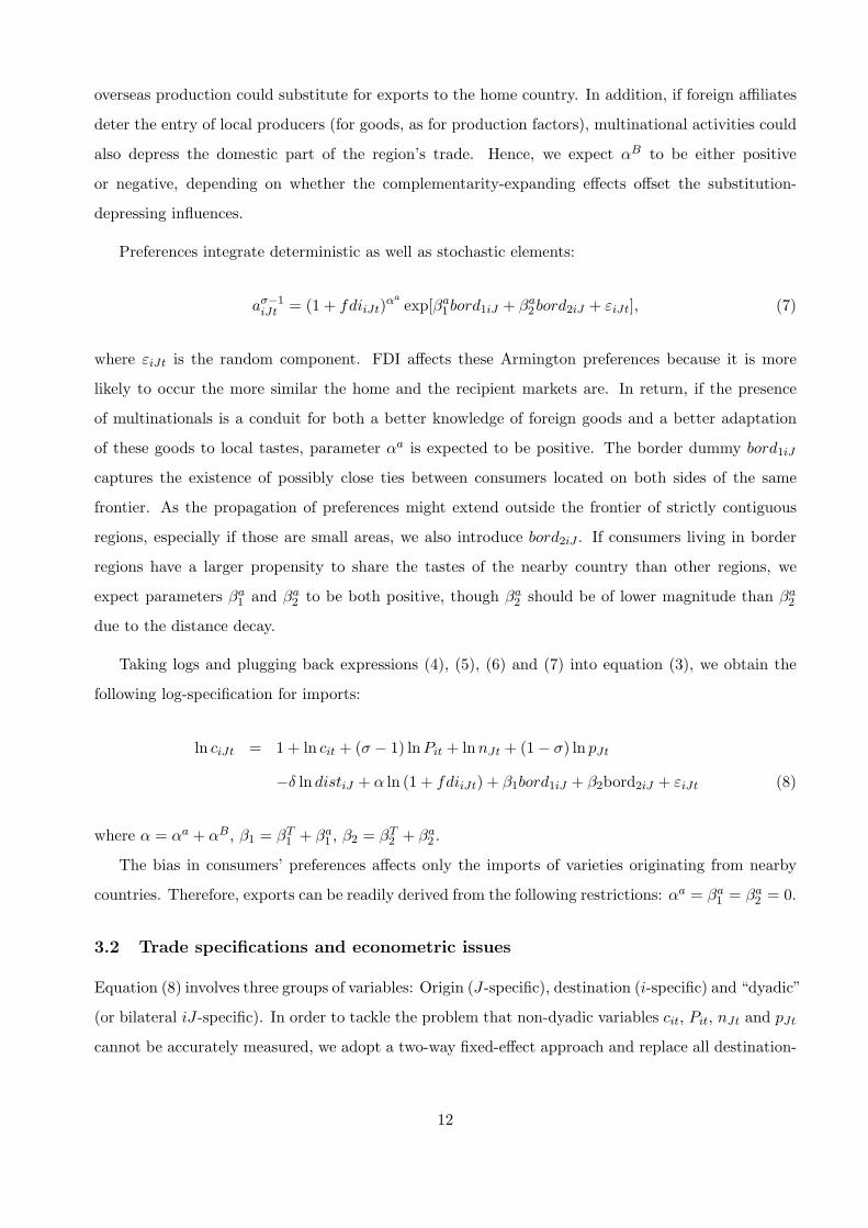
overseas production could substitute for exports to the home country. In addition, if foreign affiliates

deter the entry of local producers (for goods, as for production factors), multinational activities could

also depress the domestic part of the region’s trade. Hence, we expect αB to be either positive

or negative, depending on whether the complementarity-expanding effects offset the substitution-

depressing influences.

Preferences integrate deterministic as well as stochastic elements:

aσ−1iJt = (1 + fdiiJt)αa

exp[βa1bord1iJ + βa

2bord2iJ + εiJt], (7)

where εiJt is the random component. FDI affects these Armington preferences because it is more

likely to occur the more similar the home and the recipient markets are. In return, if the presence

of multinationals is a conduit for both a better knowledge of foreign goods and a better adaptation

of these goods to local tastes, parameter αa is expected to be positive. The border dummy bord1iJ

captures the existence of possibly close ties between consumers located on both sides of the same

frontier. As the propagation of preferences might extend outside the frontier of strictly contiguous

regions, especially if those are small areas, we also introduce bord2iJ . If consumers living in border

regions have a larger propensity to share the tastes of the nearby country than other regions, we

expect parameters βa1 and βa

2 to be both positive, though βa2 should be of lower magnitude than βa

2

due to the distance decay.

Taking logs and plugging back expressions (4), (5), (6) and (7) into equation (3), we obtain the

following log-specification for imports:

ln ciJt = 1 + ln cit + (σ − 1) lnPit + ln nJt + (1− σ) ln pJt

−δ ln distiJ + α ln (1 + fdiiJt) + β1bord1iJ + β2bord2iJ + εiJt (8)

where α = αa + αB, β1 = βT1 + βa

1 , β2 = βT2 + βa

2 .

The bias in consumers’ preferences affects only the imports of varieties originating from nearby

countries. Therefore, exports can be readily derived from the following restrictions: αa = βa1 = βa

2 = 0.

3.2 Trade specifications and econometric issues

Equation (8) involves three groups of variables: Origin (J-specific), destination (i-specific) and “dyadic”

(or bilateral iJ-specific). In order to tackle the problem that non-dyadic variables cit, Pit, nJt and pJt

cannot be accurately measured, we adopt a two-way fixed-effect approach and replace all destination-

12

specific and origin-specific variables by two groups of dummies.10 The import specification we estimate

is the following:

ln ciJt = θ + fit + fJt − δ ln distiJ + α ln (1 + fdiiJt) + β1bord1iJ + β2bord2iJ + ft + εiJt, (9)

where ft is a year-dummy capturing the unobserved time-dependent factors affecting flows identically

across regions and countries, and where fit and fJt are respectively destination- and origin-specific

dummies interacted with the previous.

Independently of trade direction, the FDI explanatory variable is potentially endogenous in equa-

tion (9), as the location choice of foreign firms is likely to depend on the trade activity itself. To

overcome this simultaneity problem, we use the method of instrument variables and estimate the

model by 2SLS. Hence, we have to find at least one variable that is partially correlated with FDI (but

not with trade), once all the other right-hand-side exogenous variables of equation (9) have been net-

ted out. Therefore, the IV candidate must be dyadic (i.e. iJ-specific), otherwise it would be strictly

collinear with either the origin or the destination fixed-effects.11 We choose the following instrument:

MP 1993iJt =

∑

k∈I(6=i)

empkJt

gtc1993ki

, (10)

where empkJt is the total employment of all the J affiliates located in region k, and gtciJ is the

generalized domestic transport cost incurred to ship manufacturing goods from region i to region k in

1993.12 Therefore, MP 1993iJt is a French market potential variable capturing the propensity of foreign

firms to locate at the vicinity of the largest affiliates from the same home country, which proved to be

highly correlated with FDI location in previous empirical studies (for instance Crozet et al., 2004). To

avoid any additional bias arising from potentially endogenous transport infrastructures (since greater

amounts of public funds might be devoted to the main FDI recipient regions), we compute market

potentials based on the value of transport costs at the beginning of the sample period, i.e. 1993.

The first-stage regression consists here in estimating the following FDI specification:

ln (1 + fdiiJt) = ρ+ fit + fJt− γ ln distiJ +φln (1 + MPiJt)+ϕ1bord1iJ +ϕ2bord2iJ + ft + ξiJt. (11)

10Empirically, including fixed-effects is actually the most widely accepted means of obtaining theory-consistent es-timates for gravity equations. See for instance Bergstrand (1985), Hummels (1999), or Anderson and van Wincoop(2003).

11In standard empirical analysis (discrete choice or gravity models), FDI specifications include a set of variablesrelated to the recipient region (local taxes, wages, GDP, ...) and to the home country. We cannot use such variables asinstruments here, because they are already captured by either fit or fJt.

12Combes and Lafourcade (2005) provide a full description of this variable.

13

The IV estimator for α derives from the following second-stage regression:

ln ciJt = θ + fit + fJt − δ ln distiJ + α [ln (1 + fdiiJt)] + β1bord1iJ + β2bord2iJ + ft + εiJt. (12)

The IV estimator is consistent under the hypothesis that the market potential and FDI variables

are effectively partially correlated. Absent additional exclusion restrictions, the model is just identified

and, therefore, condition φ 6= 0 must hold.

3.3 Definition of border regions

As noted in Section 2, caution is needed to define border regions properly. Several French border

regions, although they share a frontier with a neighboring country, do not necessarily benefit from a

direct access to this country, mostly because of physical geography (sea, mountains, ...). Therefore,

we run two sets of regressions that build on two different definitions of border regions. Firstly,

we adopt a large definition based on a simple contiguity bilateral criterion.13 We consider that all

the regions sharing a frontier with at least one neighboring country, by land or by sea, are border

regions.14 Secondly, we restrict the definition of border regions to the subset of contiguous regions

which are effectively well connected to the nearby country, i.e. the regions hosting good cross-border

transport infrastructures (major highways, tunnels or harbors).15 Using the two sets of estimates, we

can compare the trade performances of both types of border regions and quantify the contribution of

transport corridors to these performances, a prominent issue for policy-makers.

4 The trade performance of border and non-border regions

In this section, we present two sets of estimations. In the first set, presented in Section 4.1, we

analyze the trade performance of border regions relatively to interior regions over the whole period

1978-2000. Although this approach neglects the causal relationship between multinational activity

and trade, it makes possible to break down the sample into different sub-periods and to analyze

the changes in trade performances occurring throughout the successive integration episodes. By way

of contrast, Section 4.2 provides further estimates which are structurally-consistent. However, due

to data constraint, the relationship between trade performances and FDI can only be investigated

properly for the period 1993-2000.

13See Appendix B for detailed listing and mapping.14With respect to the UK, we consider all regions bordering the English Channel.15See Appendix B for detailed listing and mapping. To avoid any bias due to the possible simultaneity of trade and

infrastructure endowments, we consider only the transport infrastructures built before the period under study.

14

4.1 Baseline regressions: 1978-2000

Table 1 reports the OLS estimates derived from estimating equation (9), absent FDI in the right-hand

side explanatory variables. We consider the trade of French regions with the five neighboring countries

of France. Hence, in our estimation, the trade partner country J can only be Belgium-Luxembourg,

Germany, UK, Spain or Italy. Columns (P), (X) and (M) report the coefficients estimated over

respectively pooled flows, exports and imports.

Table 1: The average trade outperformance of French border regions

Dependent Variable: log of trade value

Border regions All contiguous Transport corridors

Model : (P) (X) (M) (P) (X) (M)

ln (dist) -0.60a -0.46a -0.74a -0.64a -0.45a -0.84a

(0.07) (0.10) (0.09) (0.06) (0.08) (0.07)

bord1 0.54a 0.33b 0.76a 0.76a 0.57a 0.96a

(0.11) (0.13) (0.16) (0.13) (0.14) (0.21)bord2 0.24a 0.12 0.35a 0.25a 0.17 0.33a

(0.07) (0.11) (0.09) (0.08) (0.11) (0.09)

N 21620 10810 10810 21620 10810 10810R2 0.879 0.904 0.921 0.881 0.906 0.923RMSE 0.579 0.520 0.520 0.575 0.515 0.515

Notes: (i) Specification estimated: ln (ciJt) = θ − δ ln (distiJ ) + β1bord1iJ +β2bord2iJ +fit +fJt +ft +εiJt. (ii) Heteroskedasticity-robust standard errorsin brackets, with a, b and c denoting significance at the 1%, 5% and 10% levels,respectively. Fixed-effects are not reported.

A first overall conclusion to be drawn from Table 1 is that, everything else equal, border regions

trade substantially more with the country with whom they share a frontier than do interior regions.

The magnitude of this trade outperformance is considerably larger for first-order than for second-order

border regions (i.e. bord1 > bord2): the former trade on average 72% more ([exp(0.54) − 1] × 100)

than interior regions, whereas the trade deviation is 27% only ([exp(0.24) − 1] × 100) for the latter.

As expected, border regions endowed with good cross-border transport connections outperform even

better, with an average trade outperformance of 114% ([exp(0.76) − 1] × 100). Trade deviations

with respect to the gravity norm are globally larger for imports than for exports, which means that

βa1 > 0 and βa

2 > 0 in equation (8). This is consistent with the model’s assumption that consumers’

preferences would be biased in favor of the differentiated goods imported from nearby countries or,

in other words, that countries would actually export more to the regions located at the other side of

their frontier than to other regions, due to “cultural” proximity.

Beyond simple average, one might wonder how relative trade performances have evolved over the

last two decades of EU integration. A dynamic perspective is even more illuminating, given that NEG

models mostly build on comparative statics and do not generally account for long-term evolutions.

15

The drawback of time-series analysis here is that different integration episodes might have affected

French trade at the same time. Indeed, although EU reforms become effective at a formal date,

their impact is actually largely anticipated, and changes are likely to occur even earlier than the

time of implementation. Therefore, we cannot reasonably capture the changes induced by integration

with a standard difference-in-difference approach. To overcome the issue of scheduling European

integration, we choose to follow trade performances throughout the period 1978-2000 and to check

whether significant changes occurred around the time of main formal reforms, that is around the

Single European Act (1986), the Schengen Agreement (1990), the Maastricht (1992) treaty, and the

successive EU enlargements to Greece (1981), Spain, Portugal (1986), Austria, Finland and Sweden

(1996). More precisely, we adopt two different approaches. First, we keep on working with trade flows

pooled over years. We thus interact border and time dummies so as to test for significant changes in

the coefficients from year to year. Secondly, we undertake further estimations based on yearly trade

sub-samples, in order to test whether the border regions located at the vicinity of the EU core exhibit

specific trends in comparison with the border regions located at the periphery of western Europe.

Table 2 reports the results of the first set of estimations. Throughout the period 1978-2000, we

observe a progressive fall in the trade outperformance of border regions. While the regions bordering

a country used to trade around twice more with this country than their interior counterparts in 1978,

they end with a lead of only 52.2% in 2000. The same declining trend is experienced by transport

corridors, whose trade outperformances were cut up by nearly a half on the same period.

Hence, the benefits of acceding to new foreign markets would be offset by the loss induced by

increasing import competition throughout the European process of integration. However, counter

forces seem to have acted against the decline by the time of two main integration episodes, that is

slightly before the Single European Act of 1986 and slightly after the Schengen Agreement of 1990.

In the second set of estimations, we proceed with year-by-year regressions over pooled over imports

and exports, for different sub-samples of partner countries. Figure 4-(a) reports the time changes in

the average trade performances of border regions, computed as [exp(β) − 1] × 100, where β is the

coefficient related to the year of estimation.16 The range of estimates is very similar to that obtained

previously. In addition, we see that the gap between well and bad connected border regions narrows

throughout the integration process (as reflected by converging thick and thin lines). The reason might

be that “gateway” regions did not experience major infrastructure improvements during the period

1978-2000, while their counterparts did.17

16Related estimation tables are available upon request. Unless mentioned, the β coefficients used to compute trade

16

Table 2: Time changes in the trade performance of French border regions

Dependent Variable: log of trade value

Border regions All contiguous Transport corridors

Model : (P) (X) (M) (P) (X) (M)

ln(dist) -0.60a -0.46a -0.74a -0.64a -0.45a -0.84a

(0.02) (0.03) (0.02) (0.02) (0.02) (0.02)bord2 0.24a 0.12a 0.35a 0.25a 0.17a 0.33a

(0.02) (0.03) (0.02) (0.02) (0.03) (0.02)

bord1 × f1978 0.67a 0.38b 0.96a 0.92a 0.73a 1.11a

(0.12) (0.15) (0.16) (0.15) (0.17) (0.22)bord1 × f1979 0.74a 0.57a 0.91a 0.94a 0.78a 1.11a

(0.11) (0.15) (0.16) (0.14) (0.18) (0.22)bord1 × f1980 0.60a 0.36a 0.83a 0.83a 0.68a 0.99a

(0.11) (0.14) (0.16) (0.14) (0.16) (0.22)bord1 × f1981 0.63a 0.44a 0.82a 0.82a 0.65a 0.99a

(0.11) (0.16) (0.17) (0.15) (0.19) (0.23)bord1 × f1982 0.64a 0.41a 0.87a 0.85a 0.64a 1.05a

(0.11) (0.15) (0.17) (0.15) (0.19) (0.23)

bord1 × f1983 0.64a 0.36b 0.93a 0.86a 0.58a 1.13a

(0.11) (0.14) (0.17) (0.15) (0.18) (0.24)

bord1 × f1984 0.57a 0.28b 0.87a 0.85a 0.58a 1.11a

(0.11) (0.13) (0.17) (0.14) (0.15) (0.24)

bord1 × f1985 0.55a 0.32b 0.78a 0.82a 0.57a 1.06a

(0.11) (0.13) (0.18) (0.14) (0.16) (0.24)

bord1 × f1986 0.55a 0.29b 0.80a 0.82a 0.53a 1.11a

(0.11) (0.13) (0.17) (0.14) (0.15) (0.22)

bord1 × f1987 0.54a 0.28b 0.81a 0.81a 0.54a 1.07a

(0.10) (0.12) (0.16) (0.13) (0.14) (0.21)

bord1 × f1988 0.53a 0.29b 0.77a 0.83a 0.59a 1.07a

(0.10) (0.12) (0.16) (0.13) (0.14) (0.21)

bord1 × f1989 0.52a 0.30b 0.73a 0.82a 0.62a 1.01a

(0.10) (0.12) (0.16) (0.12) (0.15) (0.19)

bord1 × f1990 0.48a 0.27b 0.68a 0.76a 0.57a 0.95a

(0.10) (0.13) (0.15) (0.12) (0.16) (0.19)bord1 × f1991 0.51a 0.30a 0.73a 0.77a 0.58a 0.97a

(0.10) (0.12) (0.15) (0.12) (0.15) (0.20)

bord1 × f1992 0.50a 0.28b 0.72a 0.76a 0.55a 0.96a

(0.10) (0.12) (0.16) (0.12) (0.14) (0.21)bord1 × f1993 0.52a 0.32a 0.72a 0.73a 0.51a 0.95a

(0.10) (0.10) (0.17) (0.13) (0.11) (0.23)bord1 × f1994 0.50a 0.30a 0.71a 0.68a 0.48a 0.87a

(0.09) (0.09) (0.16) (0.12) (0.10) (0.22)bord1 × f1995 0.48a 0.30a 0.66a 0.67a 0.50a 0.84a

(0.09) (0.09) (0.15) (0.12) (0.10) (0.21)bord1 × f1996 0.50a 0.34a 0.65a 0.67a 0.52a 0.83a

(0.09) (0.09) (0.15) (0.11) (0.10) (0.21)bord1 × f1997 0.47a 0.32a 0.62a 0.63a 0.47a 0.78a

(0.08) (0.08) (0.15) (0.11) (0.09) (0.21)bord1 × f1998 0.48a 0.33a 0.64a 0.60a 0.48a 0.72a

(0.09) (0.08) (0.15) (0.12) (0.10) (0.22)bord1 × f1999 0.46a 0.27a 0.65a 0.59a 0.44a 0.74a

(0.09) (0.09) (0.15) (0.12) (0.10) (0.22)bord1 × f2000 0.42a 0.32a 0.53a 0.58a 0.53a 0.63a

(0.08) (0.10) (0.12) (0.10) (0.12) (0.16)

N 21620 10810 10810 21620 10810 10810R2 0.998 0.998 0.998 0.998 0.998 0.998RMSE 0.579 0.520 0.520 0.575 0.515 0.515

Notes: Heteroskedasticity-robust standard errors in brackets, with a, b

and c denoting significance at the 1%, 5% and 10% levels, respectively.

17

To gain more insights, we divide the trade sample into the four following group of trade partner

countries. The first sub-sample, which is composed of trade with Belgium-Luxembourg and Germany,

puts the emphasis on the trends experienced by the regions bordering the EU core. The second sub-

sample adds to the previous trade with the UK, which extends the focus to the border of North-EU.

The third sub-sample includes trade with Spain and Italy in order to isolate southern border regions,

whereas the last sub-sample, which adds to the previous trade with UK provides some clue on what

is experienced at the western EU periphery.

As depicted in Figure 4-(b), absent a brief growth episode around the Single European Act of

1986, the Northern French border regions have rather stagnated over the period 1978-2000. This

stable pattern hides a recent increase in the outperformances experienced by the regions bordering

the EU core (Figure 4-(c)) and thus, a counterpart decline of the regions bordering UK. By contrast,

the trade outperformance of southern border regions fell drastically during the same period (Figure 4-

(d)), from 320% (494% for transport corridors) down to 103% (123% for transport corridors) in 2000.

As this trend still holds true, once considered the regions bordering UK (Figure 4-(e)), the depressing

prospect can be enlarged to all the border regions located at the western periphery of Europe. However,

as previously, slowdowns in the fall occur namely around the time of the Single Act, Spain’s entry

into the EU, and the Schengen agreement.

What could explain that the trade performances of French border regions depress at the western

and southern periphery of Europe, while they raise at the vicinity of the EU core ? In Section 4.2, we

investigate the role of multinationals in shaping such differentials.

4.2 The interplay between trade performances and FDI: 1993-2000

This section aims to assess the share of trade differentials explained by multinational location strate-

gies, on the period 1993-2000, for which FDI stocks are available for French regions. As in subsec-

tion 4.1, we first examine the average impact of FDI on trade performances for the whole period.

We next interact the explanatory variables with time dummies to allow effects to change over time.

Tables 3 and 4 display the results of this first set of estimations.

As a benchmark, column (B) in Table 3 reports the OLS results of estimating equation (9),

excluding FDI from the right-hand side explanatory variables, on the 1993-2000 sub-sample of flows

pooled over exports and imports. Column (P1) provides the 2SLS estimates of structural equation (12),

whereas column (P2) (respectively (P3)) interacts FDI with the first-order (respectively second-order)

deviations from the gravity norm are significantly different from zero at the level of 5% at least.17For instance, transport connections between Spain and the French border regions of “Ariege” and between Italy

and the French border region of “Alpes-de-Haute-Provence” improved respectively with the opening of the Puymorenstunnel and the Larche pass road in 1994.

18

Figure 4: Changes in the trade performances of French border regions by group of partner countries

(a) Average

(b) Northern EU border (c) Border of EU core

(d) Southern EU border (e) Border of EU periphery

19

Table 3: The average trade-expanding impact of FDI on pooled flows

Dependent Variable: log of trade value

Border regions All contiguous Transport corridors

Model : (B) (P1) (P2) (P3) (P4) (B) (P1) (P2) (P3) (P4)

ln(dist) -0.57a -0.45a -0.45a -0.44a -0.50a -0.65a -0.53a -0.51a -0.53a -0.57a

(0.03) (0.05) (0.05) (0.06) (0.07) (0.03) (0.05) (0.05) (0.07) (0.08)

bord1 0.50a 0.27a 0.56a 0.22c 0.27a 0.64a 0.31b 0.85a 0.32c 0.31b

(0.04) (0.09) (0.07) (0.12) (0.09) (0.05) (0.13) (0.12) (0.19) (0.13)

bord2 0.26a 0.23a 0.21a 0.29a 0.23a 0.22a 0.17a 0.16a 0.16b 0.18a

(0.03) (0.04) (0.04) (0.06) (0.04) (0.03) (0.04) (0.04) (0.07) (0.04)ln(1 + fdi) 0.53a 0.51a

(0.17) (0.19)ln(1 + fdi)× bord1 0.31a 0.20

(0.11) (0.13)ln(1 + fdi)× (1− bord1) 0.61a 0.61a

(0.20) (0.21)ln(1 + fdi)× bord2 0.51a 0.51a

(0.17) (0.17)ln(1 + fdi)× (1− bord2) 0.63a 0.50c

(0.23) (0.27)ln(1 + fdi)× core 0.60a 0.57a

(0.14) (0.16)ln(1 + fdi)× (1− core) 0.30 0.27

(0.31) (0.33)

N 7520 7520 7520 7520 7520 7520 7520 7520 7520 7520R2 0.857 0.845 0.841 0.838 0.852 0.858 0.846 0.841 0.846 0.853RMSE 0.559 0.582 0.589 0.595 0.568 0.557 0.580 0.589 0.579 0.566

Hausman (Prob > F ) 0.0115 0.0002 0.0071 0.0000 0.0195 0.0004 0.0012 0.0000

Note: Heteroskedasticity-robust standard errors in brackets, with a, b and c denoting significance at the 1%, 5%and 10% levels, respectively. Fixed-effects are not reported. “Hausman” provides the p-value of the Fisher test forsignificance of dξiJt in structural equation (9). A p-value < 0.05 means that the null of the FDI exogeneity is rejectedat the 5% significance level.

20

border region dummy, in order to disentangle its marginal impact between border and interior regions.

In the same spirit, column (P4) interacts FDI with a core border region dummy (defined independently

of the partner country),18 so as to assess whether trade differentials exist due to the presence of foreign

affiliates either from the nearby country, or from the other countries in the sample. Table 4 reports

similar results for the sample of respectively exports (columns (X1), (X2), (X3) and (X4)) and imports

(columns (M1), (M2), (M3) and (M4)).

As can be seen in Table 3, there is a strong positive relationship between inward multinational

activity and trade. A 10% increase in the foreign stock of affiliates entails a 5.3% increase in trade

with the parent country. This net complementarity is significantly larger for exports (8%) than for

imports (2.6%), which casts doubt on the existence of a bias in consumers’s preferences that would

be conveyed by the FDI channel. As the α estimates are not significantly different from 0 in most

import specifications, this could be evidence that border regions are mostly export platforms towards

nearby countries. In most of the estimations, we cannot reject the null of exogeneity of FDI at the 5%

significance level, which means that 2SLS are consistent estimators. Incidentally, in all the first-stage

regressions, the stock of FDI is actually partially correlated with our market potential variable, which

makes us confident in the validity of this instrument.19

More importantly, we see that augmenting the gravity specification with FDI greatly reduces

the coefficients of the bord1 variable. For the border regions defined according to a strict contigu-

ity criterion, the deviation from the gravity norm falls from 64.9% ([exp(0.50) − 1] × 100) to 31%

([exp(0.27)− 1]× 100), whereas transport corridors face a similar fall in their lead place, from 89.6%

([exp(0.64) − 1] × 100) to 36.3% ([exp(0.31) − 1] × 100). Present FDI in the gravity specification,

transport corridors do not longer outperform regarding exports. Therefore, nearly half of the trade

outperformance of first-order border regions is actually due to the presence of foreign affiliates from

the nearby country.20 However, the elasticity of trade with respect to FDI is actually significantly

larger within the group of interior regions (0.61) than within that of first-order border regions (either

0.31 or 0.20 depending on their subjacent definition). Nonetheless, we have to bear in mind that the

regions who share a frontier with a country host, on average, around 14 times more affiliates from

this country than interior regions. Therefore, although the trade-expanding effect of each additional

affiliate is larger for interior than for border regions, this is compatible with an average trade-creating

impact of FDI larger for the former than for the latter.

18Which means that “core” is a dummy taking the value 1 whenever trade observed relates to a region located at theBelgium-Luxembourg or at the German borders (whatever trade concerns these countries or not). See Appendix B fora precise listing of these regions.

19Which means that a two-tailed Student test leads to reject the null that φ = 0 in equation 11, at the 5% critical

21

Tab

le4:

The

aver

age

trad

e-ex

pand

ing

impa

ctof

FD

Ion

eith

erim

port

sor

expo

rts

Dep

enden

tV

ari

able

:lo

gflow

Bord

erre

gio

ns

All

conti

guous

Tra

nsp

ort

corr

idors

Model

:(X

1)

(M1)

(X2)

(M2)

(X3)

(M3)

(X4)

(M4)

(X1)

(M1)

(X2)

(M2)

(X3)

(M3)

(X4)

(M4)

ln(d

ist)

-0.2

8a

-0.6

2a

-0.2

8a

-0.6

2a

-0.2

5b

-0.6

2a

-0.2

8b

-0.7

1a

-0.3

0a

-0.7

5a

-0.2

9a

-0.7

3a

-0.2

8b

-0.7

8a

-0.2

9b

-0.8

6a

(0.0

8)

(0.0

6)

(0.0

8)

(0.0

6)

(0.1

0)

(0.0

7)

(0.1

1)

(0.0

9)

(0.0

8)

(0.0

6)

(0.0

9)

(0.0

7)

(0.1

1)

(0.0

8)

(0.1

3)

(0.1

1)

bord1

-0.0

40.5

8a

0.2

7a

0.8

4a

-0.1

30.5

7a

-0.0

40.5

8a

-0.1

20.7

5a

0.3

7a

1.3

3a

-0.2

10.8

5a

-0.1

20.7

4a

(0.1

3)

(0.1

1)

(0.0

8)

(0.1

3)

(0.1

8)

(0.1

5)

(0.1

3)

(0.1

2)

(0.2

0)

(0.1

7)

(0.1

1)

(0.2

5)

(0.3

1)

(0.2

5)

(0.2

0)

(0.1

9)

bord2

0.1

5a

0.3

0a

0.1

4a

0.2

9a

0.2

6a

0.3

1a

0.1

5a

0.3

1a

0.0

70.2

7a

0.0

60.2

6a

0.1

40.1

8b

0.0

60.2

9a

(0.0

5)

(0.0

5)

(0.0

5)

(0.0

5)

(0.0

8)

(0.0

7)

(0.0

5)

(0.0

5)

(0.0

6)

(0.0

5)

(0.0

6)

(0.0

5)

(0.1

0)

(0.0

9)

(0.0

7)

(0.0

6)

ln(1

+fdi)

0.8

0a

0.2

60.8

8a

0.1

4(0

.27)

(0.2

1)

(0.3

0)

(0.2

2)

ln(1

+fdi)×

bord1

0.5

7a

0.0

60.6

0a

-0.1

9(0

.16)

(0.1

5)

(0.1

9)

(0.1

9)

ln(1

+fdi)×

(1−

bord1)

0.8

8a

0.3

30.9

7a

0.2

4(0

.30)

(0.2

4)

(0.3

4)

(0.2

6)

ln(1

+fdi)×

bord2

0.7

6a

0.2

50.8

6a

0.1

6(0

.28)

(0.2

0)

(0.3

0)

(0.2

1)

ln(1

+fdi)×

(1−

bord2)

0.9

8a

0.2

91.0

0b

0.0

0(0

.37)

(0.2

7)

(0.4

6)

(0.3

3)

ln(1

+fdi)×

core

0.7

9a

0.4

1b

0.8

7a

0.2

6(0

.21)

(0.1

8)

(0.2

6)

(0.2

1)

ln(1

+fdi)×

(1−

core)

0.8

1c

-0.2

20.9

4c

-0.4

1(0

.48)

(0.4

0)

(0.5

5)

(0.4

5)

N3760

3760

3760

3760

3760

3760

3760

3760

3760

3760

3760

3760

3760

3760

3760

3760

R2

0.8

44

0.9

09

0.8

37

0.9

07

0.8

18

0.9

09

0.8

42

0.9

01

0.8

30

0.9

11

0.8

23

0.9

08

0.8

12

0.9

09

0.8

22

0.8

91

RM

SE

0.5

61

0.5

08

0.5

72

0.5

15

0.6

06

0.5

10

0.5

64

0.5

33

0.5

85

0.5

05

0.5

98

0.5

12

0.

615

0.5

09

0.5

98

0.5

56

Hausm

an

(Prob

>F

)0.0

002

0.6

140

0.0

007

0.0

057

0.0

005

0.3

218

0.0

000

0.0

000

0.0

001

0.9

949

0.0

004

0.0

053

0.0

000

0.1

427

0.0

000

0.0

000

Note

:H

eter

osk

edast

icity-r

obust

standard

erro

rsin

bra

cket

s,w

ith

a,

band

cden

oti

ng

signifi

cance

at

the

1%

,5%

and

10%

level

s,re

spec

tivel

y.Fix

ed-e

ffec

tsare

notre

port

ed.

“H

ausm

an”

pro

vid

esth

ep-v

alu

eofth

eFis

her

test

for

signifi

cance

ofd ξ iJ

tin

stru

ctura

leq

uati

ons

(9).

Ap-v

alu

e<

0.0

5m

eans

that

the

null

ofth

eFD

Iex

ogen

eity

isre

ject

edat

the

5%

signifi

cance

level

.

22

By disentangling further the effect of FDI within two additional groups, we see that not only core

border regions benefit from a larger FDI trade-creating impact on average, but also at the margin.

Indeed, the α coefficient is larger within the group of core regions (around 0.6) than elsewhere (around

0.3, but insignificant).

Finally, the distance coefficients also reduce consequently to the inclusion of FDI into the gravity

specification. Hence, distance actually captures other effects than spatial proximity, and merely

effects conveyed by variables that are negatively correlated with FDI, such as tariffs, information or

jurisdiction costs. Therefore, spatial proximity matters for trade, but in a quite complex way that

goes beyond the impact of shipment costs or “physical” geography.

Tables 5 and 6 provide further insights regarding the trade dynamics observed on the period 1993-

2000. The main explanatory variables are thus interacted with year dummies in order to show the

time trends experienced by their coefficients. As previously, in Table 5, column (B) reports the results

of estimating equation (9) (excluding FDI from the specification) on the 1993-2000 sub-sample of

pooled flows. Columns (P1), (X1) and (M1) provide the 2SLS estimates of structural equation (12) for

respectively the pooled, exports and import flows, whereas columns (P2), (X2) and (M2) (respectively

(P4), (X4) and (M4) in Table 6) disentangles the marginal impact of FDI within the group of border

and interior regions .

Column (P1) in Table 5 shows that, once controlled for inward FDI, the trade outperformance

of border regions is drastically reduced: the positive trade deviation from the gravity norm falls and

becomes insignificant for nearly all the period 1993-2000. Furthermore, the trade-creating effect of

inward FDI diminishes in magnitude (it is divided by nearly 7 from 1993 to 2000), and loses significance

over time, until becoming insignificant for the most recent years of observation. This could indicate

an increasing orientation of foreign firms towards the French market. Over time, foreign affiliates both

sell more to French consumers or firms and buy more from French suppliers, and hence, reduce their

trade with the origin country. However, this effect is not sufficiently strong to eliminate the trade

creating impact of FDI over the whole period 1993-2000. Even though horizontal motives seem to

become prevalent over time, overall, FDI appears as a complement rather than a substitute for trade.

The erosion of the trade expanding impact of foreign affiliates is lower for interior than border

regions, the FDI elasticity being divided by 5.5 on the same period. Therefore, decreasing returns to

scale in the benefits of FDI seem to prevail over the period 1993-2000.

level. Related results are available upon request.20By contrast, multinational activities only slightly affect the coefficient on second-order border regions.

23

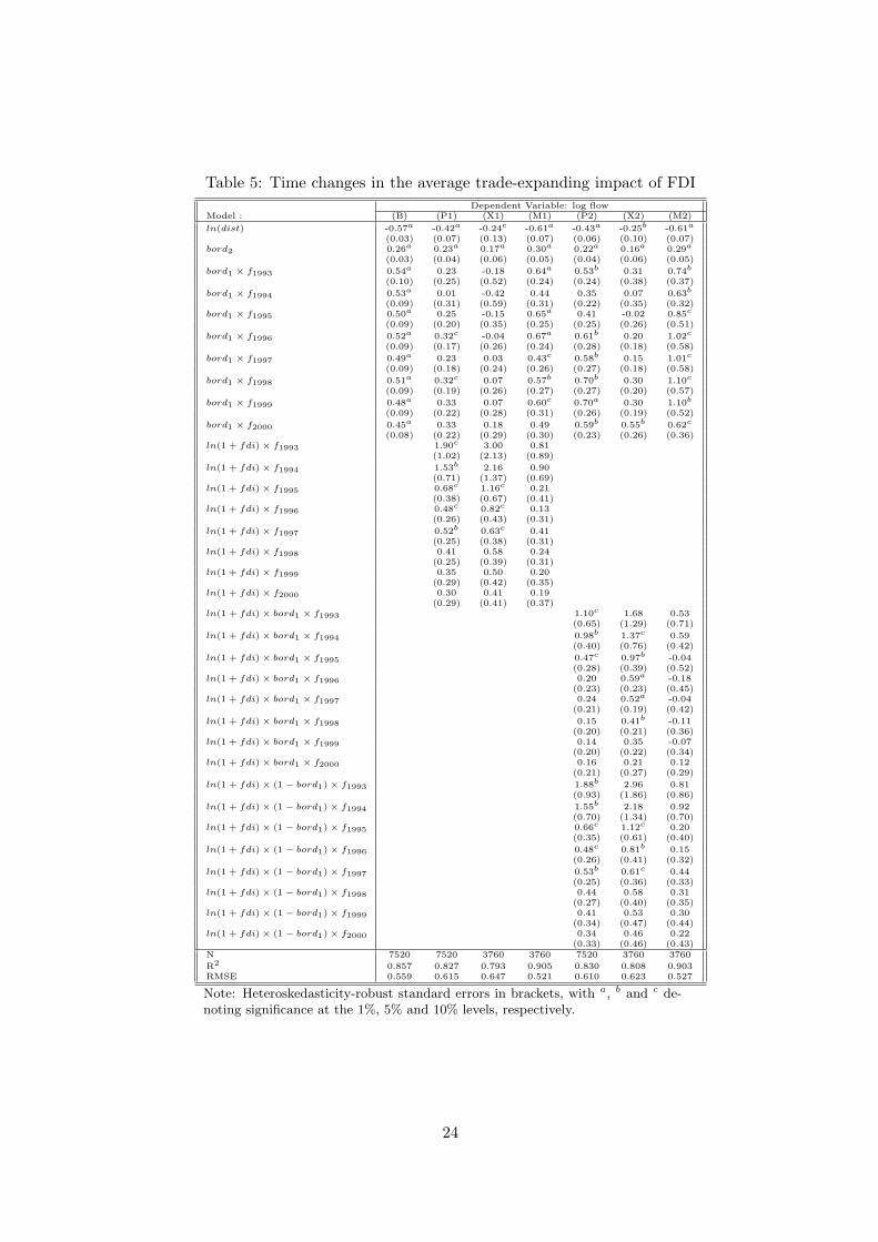
Table 5: Time changes in the average trade-expanding impact of FDIDependent Variable: log flow

Model : (B) (P1) (X1) (M1) (P2) (X2) (M2)

ln(dist) -0.57a -0.42a -0.24c -0.61a -0.43a -0.25b -0.61a

(0.03) (0.07) (0.13) (0.07) (0.06) (0.10) (0.07)bord2 0.26a 0.23a 0.17a 0.30a 0.22a 0.16a 0.29a

(0.03) (0.04) (0.06) (0.05) (0.04) (0.06) (0.05)

bord1 × f1993 0.54a 0.23 -0.18 0.64a 0.53b 0.31 0.74b

(0.10) (0.25) (0.52) (0.24) (0.24) (0.38) (0.37)

bord1 × f1994 0.53a 0.01 -0.42 0.44 0.35 0.07 0.63b

(0.09) (0.31) (0.59) (0.31) (0.22) (0.35) (0.32)bord1 × f1995 0.50a 0.25 -0.15 0.65a 0.41 -0.02 0.85c

(0.09) (0.20) (0.35) (0.25) (0.25) (0.26) (0.51)

bord1 × f1996 0.52a 0.32c -0.04 0.67a 0.61b 0.20 1.02c

(0.09) (0.17) (0.26) (0.24) (0.28) (0.18) (0.58)

bord1 × f1997 0.49a 0.23 0.03 0.43c 0.58b 0.15 1.01c

(0.09) (0.18) (0.24) (0.26) (0.27) (0.18) (0.58)

bord1 × f1998 0.51a 0.32c 0.07 0.57b 0.70b 0.30 1.10c

(0.09) (0.19) (0.26) (0.27) (0.27) (0.20) (0.57)

bord1 × f1999 0.48a 0.33 0.07 0.60c 0.70a 0.30 1.10b

(0.09) (0.22) (0.28) (0.31) (0.26) (0.19) (0.52)

bord1 × f2000 0.45a 0.33 0.18 0.49 0.59b 0.55b 0.62c

(0.08) (0.22) (0.29) (0.30) (0.23) (0.26) (0.36)ln(1 + fdi)× f1993 1.90c 3.00 0.81

(1.02) (2.13) (0.89)

ln(1 + fdi)× f1994 1.53b 2.16 0.90(0.71) (1.37) (0.69)

ln(1 + fdi)× f1995 0.68c 1.16c 0.21(0.38) (0.67) (0.41)

ln(1 + fdi)× f1996 0.48c 0.82c 0.13(0.26) (0.43) (0.31)

ln(1 + fdi)× f1997 0.52b 0.63c 0.41(0.25) (0.38) (0.31)

ln(1 + fdi)× f1998 0.41 0.58 0.24(0.25) (0.39) (0.31)

ln(1 + fdi)× f1999 0.35 0.50 0.20(0.29) (0.42) (0.35)

ln(1 + fdi)× f2000 0.30 0.41 0.19(0.29) (0.41) (0.37)

ln(1 + fdi)× bord1 × f1993 1.10c 1.68 0.53(0.65) (1.29) (0.71)

ln(1 + fdi)× bord1 × f1994 0.98b 1.37c 0.59(0.40) (0.76) (0.42)

ln(1 + fdi)× bord1 × f1995 0.47c 0.97b -0.04(0.28) (0.39) (0.52)

ln(1 + fdi)× bord1 × f1996 0.20 0.59a -0.18(0.23) (0.23) (0.45)

ln(1 + fdi)× bord1 × f1997 0.24 0.52a -0.04(0.21) (0.19) (0.42)

ln(1 + fdi)× bord1 × f1998 0.15 0.41b -0.11(0.20) (0.21) (0.36)

ln(1 + fdi)× bord1 × f1999 0.14 0.35 -0.07(0.20) (0.22) (0.34)

ln(1 + fdi)× bord1 × f2000 0.16 0.21 0.12(0.21) (0.27) (0.29)

ln(1 + fdi)× (1− bord1)× f1993 1.88b 2.96 0.81(0.93) (1.86) (0.86)

ln(1 + fdi)× (1− bord1)× f1994 1.55b 2.18 0.92(0.70) (1.34) (0.70)

ln(1 + fdi)× (1− bord1)× f1995 0.66c 1.12c 0.20(0.35) (0.61) (0.40)

ln(1 + fdi)× (1− bord1)× f1996 0.48c 0.81b 0.15(0.26) (0.41) (0.32)

ln(1 + fdi)× (1− bord1)× f1997 0.53b 0.61c 0.44(0.25) (0.36) (0.33)

ln(1 + fdi)× (1− bord1)× f1998 0.44 0.58 0.31(0.27) (0.40) (0.35)

ln(1 + fdi)× (1− bord1)× f1999 0.41 0.53 0.30(0.34) (0.47) (0.44)

ln(1 + fdi)× (1− bord1)× f2000 0.34 0.46 0.22(0.33) (0.46) (0.43)

N 7520 7520 3760 3760 7520 3760 3760

R2 0.857 0.827 0.793 0.905 0.830 0.808 0.903RMSE 0.559 0.615 0.647 0.521 0.610 0.623 0.527

Note: Heteroskedasticity-robust standard errors in brackets, with a, b and c de-noting significance at the 1%, 5% and 10% levels, respectively.

24

Table 6: Time changes in the average trade-expanding impact of FDI in core regions

Dependent Variable: log flowModel : (P4) (X4) (M4)

ln(dist) -0.45a -0.23 -0.66a

(0.11) (0.19) (0.14)

bord2 0.23a 0.16b 0.31a

(0.04) (0.06) (0.05)bord1 0.24c -0.05 0.54a

(0.13) (0.22) (0.17)ln(1 + fdi)× core× f1993 2.30c 2.88 1.71

(1.40) (2.53) (1.61)ln(1 + fdi)× core× f1994 1.14a 1.39c 0.90c

(0.44) (0.75) (0.52)

ln(1 + fdi)× core× f1995 0.76a 0.98b 0.55(0.28) (0.47) (0.34)

ln(1 + fdi)× core× f1996 0.61a 0.80b 0.42(0.23) (0.35) (0.28)

ln(1 + fdi)× core× f1997 0.58a 0.71b 0.45(0.22) (0.33) (0.29)

ln(1 + fdi)× core× f1998 0.51b 0.68b 0.35(0.21) (0.32) (0.27)

ln(1 + fdi)× core× f1999 0.46b 0.61b 0.32(0.19) (0.30) (0.25)

ln(1 + fdi)× core× f2000 0.40b 0.54c 0.26(0.19) (0.30) (0.24)

ln(1 + fdi)× (1− core)× f1993 1.70 2.96 0.44(1.18) (2.21) (1.27)

ln(1 + fdi)× (1− core)× f1994 1.41 2.38 0.45(0.92) (1.78) (0.95)

ln(1 + fdi)× (1− core)× f1995 0.52 1.19 -0.15(0.58) (0.99) (0.70)

ln(1 + fdi)× (1− core)× f1996 0.36 0.87 -0.15(0.43) (0.71) (0.53)

ln(1 + fdi)× (1− core)× f1997 0.39 0.67 0.11(0.40) (0.64) (0.48)

ln(1 + fdi)× (1− core)× f1998 0.28 0.62 -0.05(0.44) (0.71) (0.54)

ln(1 + fdi)× (1− core)× f1999 0.18 0.53 -0.17(0.57) (0.91) (0.71)

ln(1 + fdi)× (1− core)× f2000 0.11 0.56 -0.33(0.62) (0.99) (0.81)

N 7520 3760 3760R2 0.832 0.792 0.899RMSE 0.606 0.649 0.538

Note: Heteroskedasticity-robust standard errors in brackets,with a, b and c denoting significance at the 1%, 5% and 10%levels, respectively.

25

Because interior regions were initially less attractive than border regions, the decline experienced

in the gains arising from attracting new affiliates could be less pronounced for the former than for the

latter.

As can be seen in Table 6, even though core border regions experience a similar fall in FDI trade-

expanding gains throughout the period, the erosion is also less dramatic there and, most importantly,

the trade outperformance remains highly significant at the end of the period. A plausible explanation

for the drastic fall in trade outperformances suffered by the French border regions located at the

periphery of Europe would be that, during the period 1978-2000, they did not benefit from any major

cross-border transport developments, whereas their communications with the north of France (in the

form of new highways and railroad infrastructure) improved notably. Hence, the trade orientation of

these regions shifted from their neighboring countries (Spain and Italy) towards the French northern

market that was becoming more accessible overtime.

5 Conclusion

In this paper we have used an augmented gravity model to explain the geography of trade within

France, over the period 1978-2000. Firstly, we have compared the trade performances of 94 regions

according to their geographic position “vis-a-vis” a bloc of five neighboring countries of France, during

their ongoing process of integration within Europe. We find that the regions sharing a frontier with a

country trade on average as much as 70% more with this partner than other regions, once controlled

for the own region-specific and country-specific characteristics. As European integration progressed,

the French border regions located at the vicinity of the EU core succeeded in triggering new trade

surpluses, whereas those located at the western periphery of Europe did not. Even though temporary

gains were drawn from integration shocks such as the Single European Act, the Schengen Agreement

and the Maastricht Treaty, they were not sufficient to counteract the drastic long-term decline suffered

by the southern French regions bordering Spain and Italy.

Secondly, we have assessed how much of the observed trade differentials can be explained by

the location strategy of foreign affiliates from the five countries studied. The spatial distribution of

inward FDI across French regions, as its post-integration changes, explain partly these differentials.

We find that inward FDI is on average trade-expanding, independently of both the country source and

the geographic position of regions. Recalling that trade and outsourcing are complements whereas

horizontal FDI is clearly a substitute for trade, this could be evidence that FDI from French bordering

countries are mostly vertically motivated. The magnitude of the induced overtrade is larger for border

regions than for their interior counterparts. However, the marginal effect of FDI is stronger for interior

26

than for border regions, except those located at the vicinity of the EU core (e.g. at the north-eastern

frontier of Belgium-Luxembourg and Germany), which benefit from the over-representation of foreign

affiliates from all country sources. Over time the trade creating effect of inward FDI decreases. This

may indicate an increasing orientation of foreign firms towards the French market, and this trend is

even more pronounced for the Spanish and Italian affiliates.

However, inward FDI is not the only channel at work. Even once controlled for the possible

over-representation of foreign affiliates, border regions still outperform interior regions. Although it

is largely beyond the scope of this paper to properly investigate the determinants of remaining trade

differentials, simple conjectures can provide useful insights. A plausible explanation would be that a

dyadic variable distinct from inward FDI, also possibly sensitive to “proximity”, might be specifically

trade-expanding for border regions. If a first candidate is obviously outward FDI, the most plausible

candidate is migrations. As shown by a couple of empirical studies, such as Wagner et al. (2002) or

Combes et al. (2005), the preferences of immigrants might be biased towards the home country, and

their presence in a recipient region might convey better information on the trade partner country.

If border regions benefit from the over-representation of immigrants from nearby countries, due to

labor/capital complementarity (as suggested for instance by Buch et al., 2006 for German FDI), or

because of cultural, language and spatial proximity, which allow them to integrate more easily while

keeping active linkages with their family, this could generate trade over-expansion with the home

country. However, time-series data on immigration regional stocks by country source are missing and

this conjecture cannot be tested properly.

In practice, the results provided in our paper may orient the new cross-border cohesion policy

action for 2007-2013. Although European regional policies are designed to compensate for possible

post-integration inequalities, the losses suffered at the periphery of western Europe seem to have been

concealed by academic research at the benefit of eastward enlargement prospects. Policy initiatives

such as the summit of the French and Spanish governments in Zaragoza (December 2004), which has

oriented both countries’ agenda towards new cross-border infrastructure developments, would have

warranted more support in that respect.

References

Anderson, J., van Wincoop, E. (2003). Gravity with gravitas: a solution to the border puzzle.American Economic Review 93, 170-192.

Armington, P. (1969). A Theory of Demand for Products Distinguished by Place of Production.International Monetary Fund Staff Papers, 16, 159-176.

Behrens, K., Gaigne C., Ottaviano G., and Thisse J-F. (in press). Countries, regions and trade:on the welfare impacts of economic integration. Forthcoming in European Economic Review.

Behrens, K., Gaigne C., Ottaviano G., and Thisse J-F. (2006). Is remoteness a locational disad-vantage. Journal of Economic Geography, 6, 347-368.

27

Bernard, A.B., and Jensen, J.B. (1999). Exceptional Exporter Preference: cause, effect, or both?Journal of International Economics, 47, 1-25.

Bernard, A.B., Eaton, J., Jensen, J.B., and Kortum S. (2003). Plants and productivity in inter-national trade. American Economic Review, 93, 1268-1290.

Blonigen, B. (2001). In search of substitution between foreign production and exports. Journal ofInternational Economics, 53(1), 81-104.

Brainard, L. (1997). An empirical assessment of the proximity-concentration trade-off betweenmultinational sales and trade. The American Economic Review, 87(4), 520-544.

Brulhart M., Crozet, M. and Koenig-Soubeyran, P. (2004). Enlargement and the EU periphery:The impact of Changing Market Potential. World Economy, 27(6), 853-875.

Brulhart M., and Koenig-Soubeyran, P. (2006). New Economic Geography meets Comecon: re-gional wages and industry location in Central Europe. Economics of Transition, 14(2), 245-267.

Buch, C.M., Kleinert J., and Toubal F. (2006). Where enterprises lead, people follow? Linksbetween migration and FDI in Germany. European Economic Review, 50(8), 2017-2036.

Combes, P.-P., Lafourcade, M., and Mayer T. (2005). The trade-creating effects of business andsocial networks: evidence from France. Journal of International Economics, 66, 129.

Combes, P.-P., and Lafourcade, M. (2005). Transport Costs: Measures, Determinants and Re-gional Policy Implications for France. Journal of Economic Geography, 5, 319-349.

Clausing, K. (2000). Does multinational activity displace trade? Economic Inquiry, 38(2), 190-205.Combes, P.-P., Lafourcade, M., and, Mayer, T. (2005). The Trade-creating effects of Business and

Social Networks: evidence from France. Journal of International Economics, 69, 1-29.Coughlin C. C., and Wall, H.J. (2003). NAFTA and the Changing Patterns of State Exports.

Papers in Regional Science, 82(4), 427-450.Crozet, M., and Koenig, P. (2004). EU Enlargement and the Internal Geography of Countries.

Journal of Comparative Economics, 32(2), 265-279.Crozet, M., Mayer, T., and Mucchielli, J.-L. (2004). How Do Firms Agglomerate? A study of FDI

in France. Regional Science and Urban Economics, 34, 27-54.Egger, P., and Pfaffermayr, M. (2002). The Pure Effects of European Integration on intra-EU

Core and Periphery Trade. Working Paper, University of Innsbruck.Egger, P., and Pfaffermayr, M. (2004). Foreign Direct Investment and European Integration in

the 1990s. World Economy, 27(1), 99-110.Faini, R. (2004). Trade Liberalization in a Globalization World, CEPR DP 4665, London.Feenstra, R.C. (2004). Advanced international trade: Theory and evidence, Princeton University

Press, 484p.Forte, R. (2004). The relationship between foreign direct investment and international trade.

Substitution or complementarity? A survey. FEP Working Papers, 140, Universidade do Porto.Fujita, M., Krugman, P., and Venables, A.J. (1999). The Spatial Economy: Cities, Regions, and

International Trade, MIT Press, Cambridge, Massachusetts, 367p.Hanson, G. H. (1996a). Localization Economies, Vertical Organization and Trade. American

Economic Review, 86, 1266-1278.Hanson, G. H. (1996b). Economic integration, intra-industry trade, and border regions. European

Economic Review, 40, 941-949.Hanson, G. H. (1997). Increasing returns, trade and the regional structure of wages. Economic

Journal, 107, 113-133.Hanson, G. H. (2001). U.S.-Mexico integration and regional economies: evidence from border-city

pairs. Journal of Urban Economics, 50, 259-287.Head, K. and Ries, J. (2001). Overseas investment and firm exports. Review of International

Economics, 9(1), 108-122.Head K., and Mayer, T. (2004). Market Potential and the Location of Japanese Investment in the

European Union. Review of Economics and Statistics, 86(4), 959-972.

28

Helpman, E., Melitz, M.J., and Yeaple, S.R. (2004). Export versus FDI with heterogenous firms.American Economic Review, 94(1), 300-316.

Krugman, P. (1991). Increasing returns and economic geography. Journal of Political Economy,99, 483-499.

Krugman, P. and Livas Elizondo, R. (1996). Trade policy and third world metropolis. Journal ofDevelopment Economics, 49, 137-150.

Lipsey, R. and Weiss, M. (1981). Foreign production and exports in manufacturing industries.The Review of Economics and Statistics, 63, 488-494.

Lipsey, R. and Weiss, M. (1984). Foreign production and exports of individual firms. The Reviewof Economics and Statistics, 66, 304-308.

Melitz, M.J. (2003). The Impact of Trade on Intra-Industry Reallocations and Aggregate IndustryProductivity. Econometrica, 71(6), 1695-1725.

Monfort, P. and Nicolini, R. (2000). Regional convergence and international integration. Journalof Urban Economics, 48, 286-306.

Neary, J.P. (2002). Foreign Direct Investment and the Single Market. The Manchester School,70(3), 291-314.

Niebuhr, A. (2005). The Impact of EU Enlargement on European Border Regions. HWWADiscussion Paper, 330, Hamburg Institute of International Economics, Hamburg.

Niebuhr, A., and Stiller, S. (2004). Integration effects in border regions - A survey of economictheory and empirical studies. Review of Regional Research, Special Issue on Border Studies, 24(1),3-21.

Overman, H. G. and Winters, L.A. (2003). Trade shocks and industrial location: the impactof EEC accession on the UK. CEP Discussion Paper 588, Center for Economic Performance, LSE,London.

Overman, H. G. and Winters, L.A. (2005). The Port Geography of UK International Trade.Environment and Planning A, 37 (10), 1751-1768.

Paluzie, E. (2001). Trade policy and regional inequalities. Papers in Regional Science, 80, 67-85.Pfaffermayr, M. (1996). Foreign outward direct investment and exports in Austrian manufacturing:

substitutes or complements? Weltwirtschaftliches Archiv, 132(3), 501- 522.Wagner, D., Head K., and Ries J. (2002). Immigration and the trade of provinces. Scottish Journal

of Political Economy, 49(5), 507525.

Appendix A: French data sources

Trade

Each year since 1978, French decentralized customs services record the trade flows exchanged betweenthe 94 French NUTS3 regions and the different countries in the world for France. Regarding exports,the origins of trade flows are the regions where shipments are produced and loaded before handlingto destination countries, which themselves correspond to the locations where commodities are con-sumed, and conversely for import flows. The measure of trade flows obtained is therefore exclusiveof transit shipments (accounting therefore for more than 50% of the total exchanges between regionsand countries).21

The data set include trade flows (in euro values) and is originally available at a highly detailedindustry level (176 industries) and for five transport modes (air, maritime, rivers, railroad and road).22

21Data on French intra-national trade flows also exist. Unfortunately, their collection is not immune to transit andbreak-loading issues, so we cannot simply add them to customs data in order to obtain a global picture of both the intra-and international trade patterns.

22We neglect postal, pippers and other too specific shipments.

29

However, due to a change in European legislation in 1993 ruling that the mode used to transport com-modities need only be recorded when crossing European borders and not national ones, the breakdownby mode is not homogenous over the whole period of study. Therefore, we work on trade aggregatedover all the transport modes. Moreover, since the number of observations was low for some industries,we also aggregate trade over industries, which leads us to focus on trade values (instead of volumes)due to the standard problem of the units of measure.

Inward FDI

With respect to FDI, we use the data collected by the French Government Agency for InternationalInvestment (AFII).23 This agency reports yearly inward bilateral regional flows originating from 47different countries in the world, for twenty broad categories of industries.24 Moreover, five differentmeasures of FDI are available: The number of affiliates from parent firms, their employment scale(number of jobs created, of jobs maintained and total employment), and the investment value (millionseuro). The data sample for the period 1993-2000 amounts to 3900 bilateral observations.

To avoid any distortive pattern arising from the tremendous proportion of headquarters in thecapital region, we keep the flows related to three types of investments only: “Production/Assembly”,“Retail/Logistics” and “Sales offices”. Once aggregated over industries, our sample reduces to 1823bilateral observations. Finally, the flows are cumulated up to the year observed in order to obtain therelated stocks of regional FDI.25

Distance

Our distance variable corresponds to the great-circle distance between the capitals of region i andcountry J .

Appendix B: Location and definition of border regions

Figure 5 depicts the French NUTS2 and NUTS3 divisions and helps to locate the border regions wemention throughout the paper.

First-order border regions: contiguity criterion (bord1 “All contiguous”)

The easiest way to define border regions is to consider those French regions that are contiguous (byland or by sea) to their trade partner countries. This broad definition entails the following list ofNUTS3 regions:

French NUTS3 bordering Belgium-Luxembourg: Nord, Aisne, Ardennes, Meuse, Meurthe etMoselle, Moselle.

French NUTS3 bordering Germany: Moselle, Bas-Rhin, Haut-Rhin.

French NUTS3 bordering United-Kingdom (opened to the English Channel): Nord, Pas-de-Calais, Somme, Seine Maritime, Eure, Calvados, Manche, ılle-et-Vilaine, Cotes-d’Armor andFinistere.

French NUTS3 bordering Spain: Pyrenees Atlantiques, Hautes-Pyrenees, Haute-Garonne, Ariege,Pyrenees Orientales.

23See http://www.afii.fr/France/.24Among which electronics, chemicals, automobile construction and food industries are the most represented.25These could mis-approximate real FDI stocks in the case when parent firms close their affiliates meanwhile. However,

due to standard disclosure issues, we cannot control for this bias.

30

Figure 5: French NUTS2 and NUTS3 regions

French NUTS3 bordering Italy: Haute-Savoie, Savoie, Hautes-Alpes, Alpes-de-Haute-Provence,Alpes Maritimes.

First-order border regions: gateway criterion (bord1 “Transport corridors”)

We define as transport corridors those border regions that can be reached easily despite natural barriers(mountains and seas), i.e. the NUTS3 regions hosting major cross border transport infrastructures,such as highways, tunnels or industrial harbors, at the beginning of our period of study (1978). Thisdefinition leads to the following list of NUTS3 border regions:

French NUTS3 bordering Spain: Pyrenees Atlantiques (Road pass of Biriatou, highway since1975), Pyrenees Orientales (Road pass of Le Perthus, highway since 1978).

French NUTS3 bordering Italy: Haute-Savoie (Tunnel of Mont-Blanc since 1965), Savoie (Tun-nels of Frejus (road and railroad) and Mont-Cenis (railroad since 1870s), Hautes-Alpes (Roadpass of Montgenevre since 1850), Alpes Maritimes (Road pass of Tende since 1882, highway andTunnel of Vintimille since 1980).

French NUTS3 bordering United Kingdom: Pas-de-Calais (Calais harbor), Nord (Dunkerqueharbor), Seine-Maritime (Havre and Rouen harbors).

Regions bordering the EU core (core dummy)

All NUTS3 bordering Belgium-Luxembourg and Germany: Nord, Aisne, Ardennes, Meuse,Meurthe et Moselle, Moselle, Bas-Rhin, Haut-Rhin.

31