european union and no. idbtn191 united states biofuel mandates · european union and united states...
TRANSCRIPT

European Union and
United States Biofuel
Mandates
Impacts on World Markets
Perrihan Al-Riffai (IFPRI) Betina Dimaranan (IFPRI) David Laborde (IFPRI)
Inter-American
Development Bank
Sustainable Energy & Climate Change Unit, Infrastructure and Environment Sector
TECHNICAL NOTES
No. IDB-TN-191
December 2010

European Union and United States
Biofuel Mandates
Impacts on World Markets
Perrihan Al-Riffai (IFPRI) Betina Dimaranan (IFPRI)
David Laborde (IFPRI)
Inter-American Development Bank
2010

http://www.iadb.org The Inter-American Development Bank Technical Notes encompass a wide range of best practices, project evaluations, lessons learned, case studies, methodological notes, and other documents of a technical nature. The information and opinions presented in these publications are entirely those of the author(s), and no endorsement by the Inter-American Development Bank, its Board of Executive Directors, or the countries they represent is expressed or implied. This paper may be freely reproduced.
David Laborde, [email protected]

Table of Contents List of Acronyms and Abbreviations............................................................................................... i
Executive Summary ....................................................................................................................... iii 1 Introduction............................................................................................................................... 1
2 Biofuel Mandate and Trade Policies......................................................................................... 3 2.1 Brazil .................................................................................................................................4 2.2 European Union.................................................................................................................4 2.3 United States .....................................................................................................................5
3 Data and Methodology.............................................................................................................. 6
3.1 Global Database ................................................................................................................6 3.2 Global Model.....................................................................................................................9
3.2.1 Core Features of the MIRAGE Model........................................................................ 9 3.2.2 Modeling Energy and Intermediate Consumption.................................................... 12 3.2.3 Fertilizer Modeling ................................................................................................... 15 3.2.4 Modeling the Production of Biofuels........................................................................ 15 3.2.5 Modeling of Co-products and Livestock Sectors...................................................... 17
3.3 Land-use Module.............................................................................................................19 3.3.1 Land Allocation among Anthropic Activities........................................................... 20 3.3.2 Land Extension ......................................................................................................... 21
3.4 Greenhouse Gas Emissions and Land-use Change Measurement ..................................23 4 Baseline and Trade Policy Scenarios...................................................................................... 25
4.1 Sectoral and Regional Nomenclature..............................................................................25 4.2 Baseline Scenario ............................................................................................................26
4.2.1 Macroeconomic Trends ............................................................................................ 27 4.2.2 Technology ............................................................................................................... 28 4.2.3 Trade Policy Assumptions ........................................................................................ 29 4.2.4 Agri-Energy Policies................................................................................................. 31 4.2.5 Farm Policies ............................................................................................................ 32 4.2.6 Other Baseline Evolutions ........................................................................................ 32
4.3 Scenarios .........................................................................................................................33 5 Results and Discussion ........................................................................................................... 34
5.1 Production and Prices......................................................................................................35 5.1.1 Biofuel Production .................................................................................................... 35

5.1.2 Feedstock Crop Production....................................................................................... 36 5.1.3 Commodity Prices..................................................................................................... 38 5.1.4 Fuel Prices................................................................................................................. 41
5.2 Trade Impacts ..................................................................................................................42 5.2.1 Biofuel Imports ......................................................................................................... 42 5.2.2 Feedstock Trade ........................................................................................................ 43
5.3 Macroeconomic Impacts .................................................................................................44 5.3.1 Agricultural Value Added......................................................................................... 44 5.3.2 Employment.............................................................................................................. 45 5.3.3 Real Income Effects.................................................................................................. 47
5.4 Land-use Impacts ............................................................................................................49 5.5 Greenhouse Gas Emissions .............................................................................................51
6 Concluding Remarks............................................................................................................... 53 Annex I Additional Results........................................................................................................ 55
Annex II Price Changes in Partial and General Equilibrium Models....................................... 59 References..................................................................................................................................... 62
List of Tables
Table 1 MIRAGE-BIOF Land Transformation Elasticities.......................................................... 21 Table 2 Reduction of CO2 Associated with Different Feedstock ................................................. 24 Table 3 Regional Aggregation ...................................................................................................... 25 Table 4 Sectoral Aggregation ....................................................................................................... 26 Table 5 Annual Growth of Yield for Main Feedstocks and Decomposition, 2008-2020 (percentage) .................................................................................................................................. 29 Table 6 Feedstock Crop Production, 2020 (1000T and percentage change over baseline) ......... 37 Table 7 World Commodity Prices in International Markets (percentage change over baseline, 2020) ............................................................................................................................................. 39 Table 8 Food Prices in Brazil (2004=1) (percentage change over baseline) ............................... 40 Table 9 Food Prices of Commodity Aggregates (2004=1) (percentage change over baseline) .. 41 Table 10 European Union and United States Feedstock Imports by Trading Partner (percentage change over baseline) ................................................................................................................... 44 Table 11 Unskilled Labor in Brazil (Selected Sectors) (percentage change over baseline) ........ 46 Table 12 Real Wages (Skilled and Unskilled) (percentage change over baseline) ..................... 47 Table 13 Real Income and Terms of Trade (percentage change over baseline) .......................... 48

Table 14 Land Use (percentage change over baseline)................................................................ 50 Table 15 Carbon Balance over a 20-Year Period ......................................................................... 53 Table 16 Biofuel Consumption (percentage change over baseline) ............................................ 55 Table 17 European Union Biofuel Imports by Partner (percentage change over baseline)........ 56 Table 18 Biofuel Blending Rates.................................................................................................. 56 Table 19 Intensification Index for Cultivation (percentage change over baseline) .................... 57 Table 20 GDP and Welfare (percentage change over baseline) .................................................. 58
List of Figures
Figure 1 Structure of the Production Process in Agricultural Sectors in the MIRAGE-BIOF Model ............................................................................................................................................ 13 Figure 2 Biofuel Feedstock Schematic ......................................................................................... 17 Figure 3 Land-use Module............................................................................................................ 20 Figure 4 Marginal Land Extension Coefficients for Brazil .......................................................... 23 Figure 5 EU Biodiesel Imports (by source, Mtoe, baseline)......................................................... 31 Figure 6 Distribution of Biofuel Production, 2020 (by feedstock, World, baseline) .................... 32 Figure 7 Domestic Biofuel Production, 2020 ............................................................................... 36 Figure 8 Oil and Fuel Prices, 2020 ............................................................................................... 42 Figure 9 Biofuel Imports, 2020 (Mtoe,)........................................................................................ 43 Figure 10 Agricultural Value Added, 2020 .................................................................................. 45 Figure 11 Agricultural Land Extension MHa, 2020 ..................................................................... 51 Figure 12 Emissions Balance, 2020 (MTCO2eq)......................................................................... 52
List of Boxes
Box 1 Scenario Descriptions......................................................................................................... 34

Acknowledgments
This study benefitted from collaborative efforts with the Instituto de Estudos do Comércio e Negociações Internacionais (ICONE), with additional support provided by the Federação das Indústrias do Estado de São Paulo (FIESP). The initial results from this study were presented on August 9-10, 2010, at the "11º Encontro Internacional de Energia" conference, organized by FIESP in São Paulo, Brazil.


i
List of Acronyms and Abbreviations
AEZ agro-ecological zone ASEAN Association of Southeast Asian Nations
AVE ad-valorem equivalent BLUM Brazilian Land Use Model
CEPII Centre d’Etudes Prospectives et d’Informations Internationales CES constant elasticity of substitution
CET constant elasticity of transformation CGE computable general equilibrium
CO2 carbon dioxide DDA Doha Development Agenda
DDGS dried distillers grains with solubles EPA (US) Environmental Protection Agency
EU European Union FAPRI Food and Agricultural Policy Research Institute
FIESP Indústrias do Estado de São Paulo FAO Food and Agriculture Organization of the United Nations
GDP gross domestic product GHG greenhouse gas
GSP+ Generalised System of Preferences Plus GTAP Global Trade Analysis Project
HS Harmonized System ICONE Instituto de Estudos do Comércio e Negociações Internacionais
IDB Inter-American Development Bank IEA International Energy Agency
IFPRI International Food Policy Research Institute IPCC Intergovernmental Panel on Climate Change
LCA life cycle analysis LES linear expenditure system
MFN most favored nation MIRAGE Modeling International Relationships in Applied General Equilibrium
Mtoe million tons of oil equivalent

ii
OECD Organisation for Economic Co-operation and Development PEM partial equilibrium model
RED Renewable Energy Directive RFS-2 United States Renewable Fuel Standard
SAM social accounting matrix SSA Sub-Saharan Africa
T tonne TFP total factor productivity
UNFCCC United Nations Framework Convention on Climate Change UNICA União da Indústria de Cana-de-Açúcar
US United States of America

iii
Executive Summary
Biofuel production increased sharply in the past decade and can be expected to grow more
rapidly in the coming decade as national governments continue to seek greater energy
independence through renewable energy sources. A large expansion in biofuel production will be
required to meet the European Union (EU) and United States (US) biofuel consumption targets
in the next decade. These biofuel mandates will change the size and structure of global biofuel
markets and their associated sectors, and will affect consumers and producers in developed and
developing countries. The competition between biofuel crop sectors and other agricultural
commodities will have implications for agriculture and land use, especially for the net
agricultural exporting countries of Latin America. Brazil, the largest ethanol producer and
exporter in the region, has a competitive advantage due to the lower production costs and
environmental efficiency of sugarcane. The increased demand for biofuel around the world
offers both opportunities and challenges for Brazil, as well as for other developing countries.
In this study, we analyzed the potential impacts of EU and US biofuels mandates on
world biofuels markets. The evaluation focused on the impacts of the mandates on (a) the
distribution of global production, consumption and trade; (b) the prices of agricultural products
and of fuel to consumers; (c) value added, real income and terms of trade; (d) changes in land
use; and (e) the balance of emissions of greenhouse gases (GHG) associated with the liquid fuel
market, counting both the direct reduction of GHG emissions from the replacement of fossil
fuels with biofuels, as well as emissions from land-use change. Special emphasis was given to
Brazil because of the country’s importance in international ethanol markets, accounting for more
than 95% of ethanol exports in Latin America.
Building on an earlier study carried out by the International Food Policy Institute (IFPRI)
on the impacts of possible changes in EU biofuel and trade policies on global agricultural
production, trade and the environment, the impacts of EU and US biofuel and trade policies are
assessed using a global dynamic computable general equilibrium (CGE) model, which captures
domestic intersectoral relationships and interregional linkages in the global economy. The
Modeling International Relationships in Applied General Equilibrium (MIRAGE) CGE trade
model was extensively modified by IFPRI to incorporate specific features of energy demand and
ethanol and biodiesel production, including different technologies based on different feedstocks
and generation of co-products. A land supply module was also introduced, along with data on

iv
sub-national land allocation between different economic activities (forestry, pasture, different
crops) based on agro-ecological zones (AEZs). The Global Trade Analysis Project (GTAP) 7
database was modified to disaggregate key biofuel and feedstock commodities, and to ensure
consistency of the dataset in terms of prices and quantities. Instituto de Estudos do Comércio e
Negociações Internacionais (ICONE) datasets and information from the Brazilian Land Use
Model (BLUM) model were used to improve the data for Brazil.
The study shows that the incremental expansion of the biofuel consumption under the US
and EU biofuel mandates will be beneficial at the global level in terms of value addition in the
agricultural sector, in the expansion of global trade, and in the reduction of GHG emissions. The
biofuel mandates will have limited impacts on real food prices. However, there will also be
global costs driven mainly by the decline in income of oil-exporting countries.
Since both US and EU mandates favor greater ethanol consumption, it is the ethanol
sector that will expand more compared to biodiesel. Brazil will benefit from increased
production and exports of sugarcane ethanol to supply these markets, especially when the EU
and US biofuel mandates are combined with trade liberalization in biofuels in both countries, as
higher ethanol production and exports will be accompanied by higher real income gains and
agricultural value added. Use of cropland in Brazil will increase, with land coming mostly from
pasture. Unilateral biofuel trade liberalization will dampen the positive economic impacts of the
mandate for the EU and the US, but will enhance the reduction of GHG emissions as these
countries increase imports of the more environmentally efficient sugarcane ethanol. Although
Brazil will still experience real income gains when the EU and US discontinue their use of
imports of sugarcane ethanol, the gains will be sharply lower. The exclusion of sugarcane
ethanol imports will require a significant expansion of domestic ethanol production in the US
and the EU. Although more beneficial for the agricultural sector and for real income in these
countries, the mandate policy without sugarcane ethanol has more adverse implications for the
environment in terms of positive net CO2 emissions.
This study indicates that the US and EU biofuel mandates have generally beneficial impacts
on the agricultural markets and on the environment in terms of reduced CO2 emissions. These
benefits are further enhanced if the mandate policy is accompanied by liberalization in biofuel
trade. Trade liberalization will bring greater benefits to consumers in terms of lower fuel prices
and greater reductions in CO2 emissions, when sugarcane ethanol is traded. While it will result in

v
important adjustments in the agricultural sector, it will generally be beneficial for the agricultural
sector and farm producers.

1
1 Introduction
Biofuel production increased sharply in the past decade and can be expected to grow more
rapidly in the coming decade as national governments continue to seek greater energy
independence through renewable energy sources. Many countries, notably the United States (US)
and the European Union (EU), have adopted ambitious policies to reduce reliance on foreign oil
and cut down greenhouse gas (GHG) emissions. International trade in biofuel and feedstock
crops will also grow as countries seek to reach their renewable energy consumption targets
through more cost-effective and environmentally efficient means.
A large expansion in biofuel production will be required to meet the EU and US biofuel
consumption targets in the next decade. The EU adopted the Renewable Energy Directive
(RED), which includes a 10% target for the use of renewable energy in road transport fuels by
2020. Under the 2007 Energy Independence and Security Act, the US set a target of 36 billion
gallons of renewable fuels for road transportation by 2022. The renewable fuel standards are
accompanied by environmental sustainability criteria. The use of renewable fuels in the US will
be required in order to reduce GHG emissions by at least 20% by 2022, with 58% of all
renewable energy coming from cellulosic ethanol and other advanced biofuels. For the EU, the
provisions are to reduce GHG emissions by 35% by December 2010 and by 50% from 2017,
accompanied by restrictions on land where production of biofuel feedstock crops can be
established.
The US and EU biofuel mandates will change the size and structure of global biofuel
markets and its associated sectors, and will affect consumers and producers in developed and
developing countries. The competition between biofuel crop sectors and other agricultural
commodities will have implications for agriculture and land use, especially for net agricultural
exporting countries of Latin America. Brazil, the largest ethanol producer and exporter in the
region, has a competitive advantage with the lower production costs and environmental
efficiency of sugarcane. The increased demand for biofuel around the world offers both
opportunities and challenges for Brazil, as well as for other developing countries.
In this study, we seek to clarify the interactions between different biofuel policy scenarios
and their potential impacts on global agricultural markets and on the environment, particularly on
production, trade, welfare, land use and CO2 emissions. The primary goal of the study is to
analyze the potential impacts of the EU and US biofuels mandates on world biofuels markets.

2
We focus on Brazil, and not on other developing countries in Latin America or other regions,
because of the importance of Brazil in international ethanol markets. For example, within Latin
America, Brazil accounts for more than 95% of ethanol exports. This is amplified in some
countries in the region, especially those in Central America and the Caribbean, where most of the
ethanol exports are re-exports from Brazil.
This evaluation focuses on the impacts of the mandates on (a) the distribution of global
production, consumption and trade; (b) the prices of agricultural products and of fuel to
consumers; (c) value added, real income and terms of trade; (d) changes in land use; and (e) the
balance of emissions of GHGs associated with the liquid fuel market, counting both the direct
reduction of GHG emissions from the replacement of fossil fuels with biofuels, as well as
emissions from land-use change.
Although the study covers both the biodiesel and ethanol markets, the study provides
greater emphasis on the evaluation of impacts of policies on the ethanol market. This emphasis
on ethanol arises from the greater expansion in ethanol, relative to the biodiesel market, that
results from both the US and EU mandates, and the concentration of initial high levels of trade
protection in the sector. With the stronger slant towards ethanol and the acknowledged
importance of Brazil in the global biofuel market, this study also analyses the hypothetical
impacts of limited consumption of sugarcane ethanol on the US and EU markets, including the
impacts of biofuel consumption targets on GHG emissions.
This study builds on an earlier International Food Policy Research Institute (IFPRI) study
by Al-Riffai, Dimaranan, and Laborde (2010) that analyzes the impact of possible changes in EU
biofuel and trade policies on global agricultural production and the environmental performance
of the EU biofuel policy as concretized in the RED. The quantitative analysis of the global
economic and environmental impact of first-generation biofuel development was conducted
using an extensively modified version of the Modeling International Relationships in Applied
General Equilibrium (MIRAGE) global, dynamic computable general equilibrium (CGE)
model1, which captures domestic intersectoral relationships and interregional linkages in the
global economy. Primary among the major methodological innovations introduced in this new
MIRAGE model (MIRAGE-BIOF) is the new modeling of energy demand, which allows for
1 The MIRAGE model was initially developed at the Centre d’Etudes Prospectives et d’Informations Internationales (CEPII). Documentation of the standard model is available in Bchir et al. (2002) and Decreux and Valin (2007).

3
substitutability between different sources of energy, including biofuels. This is facilitated by the
extension of the underlying Global Trade Analysis Project (GTAP) database, which separately
identifies ethanol with four subsectors, biodiesel, five additional feedstock crop sectors, four
vegetable oils sectors, fertilizers and the transport fuel sectors. The model was also modified to
account for co-products generated in the ethanol and biodiesel production processes and their
role as inputs to the livestock sector. Fertilizer modeling was also introduced to allow for
substitution with land under intensive or extensive crop production methods. Finally, another
major innovation is the introduction of a land use module, which allows for substitution between
land classes, classified according to AEZs and land-extension possibilities. This land-use module
enables assessment of the GHG emissions (focusing on CO2) associated with land-use changes.
In this study commissioned by the Inter-American Development Bank (IDB), the
MIRAGE-BIOF model was further improved with data for Brazil obtained from Brazil’s
Institute for International Trade Negotiations, including information from the Brazilian Land Use
Model (BLUM)2.
A brief review of biofuel policies in the EU, US and Brazil is provided in the next section
of the report. Section 3 includes an overview of the data development and model development
involved in the study. Readers are referred to Al-Riffai et al. (2010) for more detailed
discussions on the various components of the methodology. The baseline scenario and alternative
trade policy scenarios analyzed in the study are presented in Section 4. Results and discussions
are provided in Section 5, and concluding remarks are given in Section 6.
2 Biofuel Mandate and Trade Policies
In recent years, many countries have instituted biofuel programs due to the need to reduce
reliance on foreign fossil fuels and to achieve energy independence, to bolster farm incomes, and
to reduce GHGs. This section provides a brief background about the biofuel policies in the three
main biofuel markets: Brazil, the EU, and the US.
2 Technical discussions with, and data support from, Andre Nassar of the Instituto de Estudos do Comércio e Negociações Internacionais (ICONE) are gratefully acknowledged.

4
2.1 Brazil
Ethanol policies have been implemented in Brazil since the mid-70s and current blending
obligations for ethanol are up to 20-25% for gasoline. More recently, Brazil has introduced
biodiesel blending targets of 2% in 2008 and 5% in 2013, similar to the EU. In order to reach
these obligations, Brazilian federal and state governments grant tax reductions/exemptions. The
level of advantage varies based on the size of the agro-producers and on the level of development
of each Brazilian region.
The Common External Tariff of Mercosur also protects domestic biofuel production, with
ethanol duties of 20% and biodiesel duties of 14%. These tariffs could be eliminated or
significantly reduced under the Doha and/or the EU-Mercosur negotiations. Furthermore, no
non-tariff barriers constrain Brazilian imports of biofuels (e.g. no tariff-rate quota on biofuels in
Mercosur).
Another important explanatory factor in the growth of the ethanol sector in Brazil is the
role of foreign investment with recent investments coming from Europe and the United States.
The investments include not only distillation plants, but also sugarcane production. The
competitive prices of raw materials and the high level of integration in the process explain the
lower costs for ethanol production in Brazil and the motivation of the foreign investors.
2.2 European Union
The adoption of targets for the use of biofuels in road transport fuels is a key component of the
EU’s response to achieving its Kyoto targets of GHG emissions. In 2003, the EU first set a target
of 5.75% biofuels use in all road transport fuels by the end of 2010. The proposal to adopt a 10%
target for a combination of first and second generation biofuels use in road transport fuels by
2020 was made in the Renewable Energy Roadmap (CEC, 2006) as part of an overall binding
target for renewable energy to represent 20% of the total EU energy mix by the same date. On 23
April 2009, the EU adopted the RED, which includes a 10% binding target for renewable energy
use in road transport fuels and also establishes the environmental sustainability criteria for
biofuels consumed in the EU (CEC, 2008). A minimum rate of GHG emission savings (35% in
2009 and rising over time to 50% in 2017), rules for calculating GHG impact, and restrictions on
land where biofuels may be grown are part of the environmental sustainability scheme that
biofuel production must adhere to under the RED. The revised Fuel Quality Directive, adopted at

5
the same time as the RED, includes identical sustainability criteria and it targets a reduction in
lifecycle GHG emissions from fuels consumed in the EU by 6% by 2020. The adoption of the
RED includes a requirement for the Commission to report, by 31 December 2010, on the impact
of indirect land-use change on GHG emissions and ways to minimize that impact.
EU trade policies also affect domestic biofuel production and reduce production
incentives and export opportunities for foreign biofuel producers (e.g. US, Brazil, Indonesia,
Malaysia, etc.). The most-favored-nation (MFN) duty for biodiesel is 6.5%, while for ethanol
tariff barriers are higher (€19.2 / hectolitre for the HS6 code 2207103 and €10.2 / hectolitre for
the code 220720). Even if tariffs for biodiesel were to be reduced, trade would still have to face
more restrictive non-tariff barriers in the form of quality and environmental standards, which
already mostly affect developing country exporters.
Nevertheless, some European partners already benefit from a duty-free access for
biofuels under the Everything But Arms Initiative, the Cotonou Agreement, the Euro-Med
Agreements and the Generalised System of Preferences Plus (GSP +). Many ethanol exporters,
such as Guatemala, South Africa and Zimbabwe, use this free access opportunity. However,
most ethanol imports come from Brazil and Pakistan under the ordinary European GSP without
any preference for either since 2006. For European biofuel exports, the EU has a preferential
access for ethanol in Norway through tariff-rate quotas (i.e. 164 thousand hectolitres for code
220710 and 14.34 thousand hectolitres for 220720).
2.3 United States
US biofuel policies date back to the 1970s and are as complex as those of the EU. Fiscal
incentives and mandates vary from one state to another and differ from those at the federal level.
The Energy Tax Act of 1978 introduced tax exemptions and subsidies for the blending of ethanol
in gasoline. In contrast, biodiesel subsidies are more recent and were introduced in 1998 with the
Conservation Reauthorization Act.
Mandates on biofuel consumption were initiated under the Energy Policy Act of 2005 at
the federal level, although obligations for biofuel use exist at the state level (e.g. Minnesota
introduced a mandate on biofuels before the federal government, which it increased to 20% in
3 Harmonized System (HS) code 220710 refers to undenatured ethyl alcohol, of actual alcoholic strength of 80%; HS 220720 refers to denatured ethyl alcohol and other spirits.

6
2013). This 2005 Act set the objective of purchasing 4 billion gallons of biofuels in 2006 and 7.5
billion gallons in 2012.
The US Renewable Fuel Standard (RFS-2) provides volume targets for different kinds of
biofuel. The US mandate implies consumption of 1 billion gallons of biodiesel (3.15 Mtoe
[million tons of oil equivalent]), 3.5 billion gallons of non-cellulosic advanced biofuels (7 Mtoe),
and 15 billion gallons of conventional biofuels (30 Mtoe) by 2020.
The current biofuels policies in the US consist of three main tools: output-linked
measures, support for input factors and consumption subsidies. Tariffs and mandates benefit
biofuels producers through price support. Tariffs on ethanol (24% in ad-valorem equivalent
[AVE]) are higher than biodiesel (1% in AVE), which limit imports, especially from Brazil.
Moreover, producers benefit from tax credits based on biofuels blended into fuels. The
Volumetric Ethanol Excise Tax Credit and the Volumetric Biodiesel Excise Tax Credit provide
the single largest subsidies to biofuels, although there are additional subsidies linked to biofuel
outputs.
3 Data and Methodology
This study uses the MIRAGE-BIOF model and the dataset developed for the study entitled
“Global Trade and Environmental Impact Study of the EU Biofuels Mandate“ (Al-Riffai,
Dimaranan, and Laborde, 2010). Several changes in parameter values and in the dataset have
been performed in this study thanks to the contribution of the Instituto de Estudos do Comércio e
Negociações Internacionais (ICONE) and information from the Brazilian Land Use Model
(BLUM), which improved the data for Brazil. In the description of the database and model used
in this study, we emphasize the main changes from the previous study.
3.1 Global Database
The MIRAGE model relies on the Global Trade Analysis Project (GTAP) database for global,
economy-wide data. The GTAP database combines domestic input-output matrices, which
provide details on the intersectoral linkages within each region, and international datasets on
macroeconomic aggregates, bilateral trade, protection and energy. We started from the latest
available database, GTAP 7, which describes global economic activity for the 2004 reference
year in an aggregation of 113 regions and 57 sectors (Narayanan and Walmsley, 2008). The
database was then modified to accommodate the sectoral changes made to the MIRAGE model.

7
Twenty-three new sectors were carved out of the GTAP sector aggregates – the liquid
biofuels sectors (an ethanol sector with four feed-stock specific sectors, and a biodiesel sector),
major feedstock sectors (maize, rapeseed, soybeans, sunflower, palm fruit and the related oils),
co- and by-products of distilling and crushing activities, the fertilizer sector and the transport
fuels sector. For the last two sectors, we split the existing GTAP sectors with the aid of the
SplitCom software.4
However, after several tests, we found that the limitations of the SplitCom software and
the initial data lead to very unsatisfactory results in the splitting of several feedstock crops,
vegetable oils and biofuel sectors. We therefore developed an original and specific procedure to
generate a database that is consistent in both values and quantities. The general procedure is as
follows:
• Agricultural production value and volume are targeted to match Food and Agriculture
Organization of the United Nations (FAO) statistics. A world price matrix for
homogenous commodities was constructed in order to be consistent with international
price distortions (transportation costs, tariffs, and export taxes or subsidies).
• Production technology for new crops is inherited from the parent GTAP sector and the
new sectors are deducted from the parent sectors.
• New vegetable oil sectors are built using a bottom-up approach based on crushing
equations. Value and volume of both oils and meals are consistent with the prices matrix,
physical yields and input quantities.
• Biofuel sectors are built using a bottom-up approach to respect the production costs, input
requirements, production volume, and for the different type of ethanols, the different by-
products. Finally, rates of profits are computed based on the difference between
production costs, subsidies and output prices.
• For Steps 2, 3, and 4, the value of inputs is deducted from the relevant sectors (other food
products, vegetable oils, chemical and rubber products, fuel) in the original social
accounting matrix (SAM), allowing resources and uses to be extracted from different
sectors if needed (n-to-n). 4 SplitCom, a Windows program developed by J. Mark Horridge of the Center for Policy Studies, Monash University, Australia, is specifically designed for introducing new sectors in the GTAP database by splitting existing sectors into two or three sectors. Users are required to supply as much available data on consumption, production technology, trade, and taxes either in US dollar values or as shares information for use in splitting an existing sector. The software allows for each GTAP sector to be split one at a time, each time creating a balanced and consistent database that is suitable for CGE analysis.

8
• At each stage, consumption data are adjusted to be consistent with production and trade
flows.
It is important to emphasize that this procedure, even if time consuming and delicate to operate
with so many new sectors, was crucial and differs from a more simplistic approach used in the
literature until now. Indeed, each step allows us to address several issues. For instance, Step 1
allows us to have a more realistic level of production compared to the GTAP database wherein
production targeting is done only for Organisation for Economic Co-operation and Development
(OECD) countries, with some flaws, and therefore has an outdated agricultural production
structure for many countries. Building a consistent dataset in value and volume – thanks to the
price matrix – is also critical. Targeting only in value often generates inconsistencies in the
physical linkage that thereby leads to erroneous assessments (e.g. wrong yields for extracting
vegetable oil). Even more important is the role of initial prices, and price distortions, in a
modeling framework using constant elasticity of substitution (CES) and constant elasticity of
transformation (CET) functions. Indeed, economic models rely on optimality conditions and, in
our case, as in all the CGE literature, our modeling approach leads to equalization of the
marginal rate of substitution (CES case) to relative prices. It means that the physical conversion
ratio is bound to the relative prices. Wrong initial prices, or incorrect price normalization, will
lead to convert X units of good i (e.g. imported ethanol) into Y units of good j (e.g. domestic
produced ethanol). In the case of a homogenous good, we need to have an initial price ratio equal
to one and to ensure with a high elasticity of substitution that this ratio will remain close to one.
Otherwise, misleading results appear (e.g. one ton of palm oil will replace only half a ton of
sunflower oil, one ton of imported ethanol can replace 1.5 tons of domestic ethanol). This
mechanism may be neglected in many CGE exercises where the level of aggregation easily
explains the imperfect substitution. In the case of this study, however, we found it imperative to
directly address this challenge since we deal with a high level of sector disaggregation, a high
level of substitution (among ethanols produced from different feedstocks, among vegetable oils,
or among imported and domestic production), and with the critical role of physical linkages,
from the crop areas to the energy content of different fuels and meals.
Finally, a flexible procedure is needed (Step 5) since some of our new sectors can be
constructed from among several sectors in GTAP. SplitCom allows only a 1-to-n disaggregation,
which is rather restrictive for the more complex configuration that we face with the data. For

9
instance, Brazilian ethanol trade data falls under the beverages and tobacco sector while its
production is classified under the chemical products sector. For the vegetable oils, we face
similar issues since the value of the oil is in the vegetable oil sector but the value of the oil meals
are generally under in the food products sector.
The specific data sources, procedures and assumptions made in the construction of each
new sector are described in Al-Riffai, Dimaranan, and Laborde (2010, Annex I).
3.2 Global Model
The MIRAGE model (Decreaux and Valin, 2007), a CGE model originally developed at Centre
d’Etudes Prospectives et d’Informations Internationales (CEPII) for trade policy analysis, was
extensively modified at IFPRI in order to address the potential economic and environmental
impact of biofuels policies. The key adaptations to the standard model are the integration of two
main biofuels sectors (ethanol and biodiesel) and biofuel feedstock sectors, improved modeling
of the energy sector, the modeling of co-products and the modeling of fertilizer use. The land-use
module which includes the decomposition of land into different land uses, and the quantification
of the environmental impact of direct and indirect land-use change, was introduced in the model
at the AEZ level, allowing for infra-national modeling. The latter feature is particularly valuable
for large countries such as Brazil where production patterns and land availability are quite
heterogeneous.
Extensive model modifications were done by Al-Riffai, Dimaranan, and Laborde (2010)
to adapt the MIRAGE trade policy-focused CGE model for an assessment of the trade and
environmental impacts of biofuels policies. Some of the changes made to the model were
previously introduced by Bouët et al. (2008) and Valin et al. (2009). In this section, we provide a
brief description of the main features of the MIRAGE model. This is followed by the adaptations
and innovations made in the areas of energy modeling, the modeling of co-products of ethanol
and biodiesel production, and the description of fertilizer use. More detailed explanations of the
various modeling changes are provided in the annex to this report.
3.2.1 Core Features of the MIRAGE Model This section summarizes the features of the standard version relevant for this study. MIRAGE is
a multisector, multiregion CGE Model for trade policy analysis. The model operates in a
sequential dynamic recursive set-up: it is solved for one period, and then all variable values,

10
determined at the end of a period, are used as the initial values of the next one. Macroeconomic
data and SAMs, in particular, come from the GTAP 7 database (see Narayanan, 2008), which
describes the world economy in 2004. From the supply side in each sector, the production
function is a Leontief function of value added and intermediate inputs: one output unit needs for
its production x percent of an aggregate of productive factors (labor, unskilled and skilled;
capital; land and natural resources) and (1 – x) percent of intermediate inputs.5 The intermediate
inputs function is an aggregate CES function of all goods: it means that substitutability exists
between two intermediate goods, depending on the relative prices of these goods. This
substitutability is constant and at the same level for any pair of intermediate goods. Similarly, in
the generic version of the model, value added is a CES function of unskilled labor, land and
natural resources, and of a CES bundle of skilled labor and capital. This nesting allows the
modeler to introduce less substitutability between capital and skilled labor than between these
two and other factors. In other words, when the relative price of unskilled labor is increased, this
factor is replaced by a combination of capital and skilled labor, which are more complementary.6
Factor endowments are fully employed. The only factor whose supply is constant is
natural resources. Capital supply is modified each year because of depreciation and investment.
Growth rates of labor supply are fixed exogenously. Land supply is endogenous; it depends on
the real remuneration of land. In some countries land is a scarce factor (for example, Japan and
the EU), such that elasticity of supply is low. In others (such as Argentina, Australia, and Brazil),
land is abundant and elasticity is high7.
Skilled labor is the only factor that is perfectly mobile. Installed capital and natural
resources are sector specific. New capital is allocated among sectors according to an investment
function. Unskilled labor is imperfectly mobile between agricultural and nonagricultural sectors
following a constant CET function: unskilled labor’s remuneration in agricultural activities
differs from that in nonagricultural activities. This factor is distributed between these two series
of sectors according to the ratio of remunerations. Land is also imperfectly mobile amongst
agricultural sectors.
5 The fixed-proportion assumption for intermediate inputs and primary factor inputs is especially pertinent to developed economies, but for some developing economies that are undergoing dramatic economic growth and structural change, such as China, the substitution between intermediate inputs and primary factor inputs may be significant. 6 In the generic version, substitution elasticity between unskilled labor, land, natural resources and the bundle of capital and skilled labor is 1.1; it is only 0.6 between capital and skilled labor. This structure has been modified for the present exercise. 7 This assumption, which applies to the standard model, is modified in the version of MIRAGE used in this biofuels study (MIRAGE-BIOF).

11
In the MIRAGE model there is full employment of labor; more precisely, there is
constant aggregate employment in all countries, combined with wage flexibility. It is quite
possible to suppose that total aggregate employment is variable and that there is unemployment;
but this choice greatly increases the complexity of the model, so that simplifying assumptions
have to be made in other areas (such as the number of countries or sectors). This assumption
could amplify the benefits of trade liberalization for developing countries: in full-employment
models, increased demand for labor (from increased activity and exports) leads to higher real
wages, such that the origin of comparative advantage is progressively eroded; but in models with
unemployment, real wages are constant and exports increase much more.
Capital in a given region, whatever its origin, domestic or foreign, is assumed to be
obtained by assembling intermediate inputs according to a specific combination. The capital
good is the same whatever the sector. MIRAGE describes imperfect, as well as perfect,
competition. In sectors under perfect competition, there is no fixed cost, and price equals
marginal cost.
The demand side is modeled in each region through a representative agent whose
propensity to save is constant. The rest of the national income is used to purchase final
consumption. Preferences between sectors are represented by a linear expenditure system–
constant elasticity of substitution (LES-CES) function. This implies that consumption has a non-
unitary income elasticity; when the consumer’s income is augmented by x percent, the
consumption of each good is not systematically raised by x percent, other things being equal.
The sector sub-utility function used in MIRAGE is a nesting of four CES functions. In
this study, Armington elasticities are drawn from the GTAP 7 database and are assumed to be the
same across regions. But a high value of Armington elasticity, i.e. 20, is assumed for all
homogenous sectors (single crops, single vegetable oils, ethanol).8 For biodiesel, we assume the
same elasticity as that for other fossil fuels.
Macroeconomic closure is obtained by assuming that the sum of the balance of goods and
services and foreign direct investments is constant in terms of share of the world gross domestic
product (GDP).
8 Compared to 10 in the “Global Trade and Environmental Impact Study of the EU Biofuels Mandate” study.

12
3.2.2 Modeling Energy and Intermediate Consumption
The most significant of these model modifications is the modeling of the energy sector to
introduce energy products, including biofuels, as components of value-added in the production
process. Following a survey of energy modeling approaches, the MIRAGE model was modified
following a top-down approach, similar to the approach taken with the GTAP-E model
(Burniaux and Truong, 2002), wherein energy demand is derived from the modeling of
macroeconomic activity. However, beyond what is in the GTAP-E model, the MIRAGE model
was revised to include a better representation of agricultural production processes to better
capture the potential impact of biofuels development on agricultural production (see Figure 1).
The paper by Burniaux and Truong (2002) was the inspiration for the elasticities of
substitution of the different CES nesting levels described above. The elasticities of substitution
are set at 1.1 between energy and electricity, 0.5 between energy and coal, and 1.1 between fuel
oil and gas. Based on estimates from Okagawa and Ban (2008) (EU KLEMS estimates), the
elasticity of substitution between capital and energy is 0.2 in industry, 0.3 in services and 0.03 in
agriculture.

13
Figure 1 Structure of the Production Process in Agricultural Sectors in the MIRAGE-BIOF Model
Source: Bouët, A., B. Dimaranan, and H. Valin (2010)
Finally, it is worth noting that a distinctive feature of this new version of MIRAGE is in
the grouping of intermediate consumptions into agricultural inputs, industrial inputs and services
inputs. This introduces greater substitutability within sectors. For example, substitution is higher
between industrial inputs (substitution elasticity of 0.6) than between industrial and services
inputs (substitution elasticity of 0.1). At the lowest level of demand for each intermediate input,
firms can compare the prices of domestic and foreign inputs and for the latter, the prices of these
foreign inputs coming from different regions. In non-agricultural sectors demand for energy
exhibits specific features that are incorporated as follows:
• In the transportation sectors (road transport and air and sea transport) the demand for
fuel, which is a CES composite of fossil fuel, ethanol and biodiesel, is less substitutable.
The modified value added is a CES composite with very low substitution elasticity (0.1)
between the usual composite (unskilled labor and a second composite, which is a CES of

14
skilled labor and a capital and energy composite) and fuel, which is a CES composite
with high elasticity of substitution (1.5) of ethanol, biodiesel and fossil fuel.
• In sectors that produce petroleum products, intermediate consumption of oil has been
made nearly fixed. The modified intermediate consumption is a CES composite (with low
elasticity, 0.1) of a composite of agricultural commodities, a composite of industrial
products, a composite of services and a composite of energy products. The latter
composite is a CES function (with low elasticity) of oil, fuel (composite of ethanol,
biodiesel, and fossil fuel with high elasticity, 1.5) and of petroleum products other than
fossil fuel. The share of oil in this last composite is by far the largest one. This implies
that when demand for petroleum products increases, demand for oil increases by nearly
as much.
• In the gas distribution sector, the demand for gas is made less substitutable. It has been
introduced at the first level under the modified intermediate consumption composite, at
the same level as agricultural inputs, industrial inputs and services inputs. This CES
composite is introduced with a very low elasticity of substitution (0.1).
• In all other industrial sectors we keep the production process illustrated in Figure 1,
except that there is no land composite, and fuel is introduced in the intermediate
consumption of industrial products.
In addition to the extensive modifications made to address the shortcomings of the
MIRAGE global trade model in characterizing the energy sector, modifications were also made
in the MIRAGE demand function for final consumption. The LES-CES, which captures non-
homothetic behaviour in response to changes in income, was improved through the introduction
of new calibration to USDA income and price elasticities (Seale et al., 2003). For China and
India, some complementary information was sourced from the Food and Agricultural Policy
Research Institute (FAPRI). The LES-CES demand structure was further modified to allow for a
separate characterization of demand for fuel relative to demand for other goods. A new LES-
CES level is introduced to allow for the lower elasticity of fuel demand to prices. Further details
on this modification of the energy demand structure is provided in Annex III in Al-Riffai,
Dimaranan, and Laborde (2010). The elasticity of substitution at this level is calibrated to obtain
fuel consumption in the baseline consistent with energy model projections (e.g. the EU PRIMES
model). The value for all regions is 0.4.

15
Compared to previous studies, we have devoted more attention to the Brazilian demand
for ethanol. Due to the specificity of the Brazilian market with the flex fuel car fleet, the
possibility of substitution between gasoline and ethanol is larger in this country. This substitution
is represented by a CES function with an elasticity of 2.6. This elasticity has been calibrated to
target in the baseline the central demand scenario of ethanol projected by União da Indústria de
Cana-de-Açúcar (UNICA) (2010).
3.2.3 Fertilizer Modeling Fertilizers are explicitly introduced in the global database and MIRAGE-BIOF model to capture
potential crop production intensification with use of more fertilizers, in response to increased
demand for biofuel feedstock crops. The characterization of the crop production response to
prices resulting from increased bioenergy demand is particularly important. Through improved
modeling of fertilizers and their impact on crop yield, we introduce a more realistic
representation of yield responses to economic incentives while taking into account biophysical
constraints and saturation effects using a logistic approach. The degree of crop intensification
depends on the relative price between land and fertilizers. Further details on fertilizer modeling
in MIRAGE-BIOF are provided in Al-Riffai, Dimaranan, and Laborde (2010, Annex IV).
In this context, crop yields in the model may increase through three channels:
1. Exogenous technical progress (see baseline section);
2. Endogenous “factor” based intensification: land is combined with more labor and
capital;
3. Endogenous “fertilizers” (intermediate consumption) based intensification, the
mechanism described above.
The model does not include endogenous technical progress based on private or public research
and development expenditures in response to relative price changes. However, the increase of
capital and labor by unit of land (effect ii) plays a similar role.
3.2.4 Modeling the Production of Biofuels The biodiesel and ethanol sectors are modeled in slightly different ways. Biodiesel
production, which does not produce by-products, uses four kinds of vegetable oils (palm oil,
soybean oil, sunflower oil and rapeseed oil) as primary inputs (see Figure 2). These are
combined with other inputs (mainly chemicals and energy) and value added (capital and labour).

16
Intermediate consumption is modeled using a CES nested structure with high substitutability
assumed among the vegetable oils (an elasticity of substitution equal to 8). The initial dataset and
the calibration of the model were set to allow for an initial marginal rate of substitution equal to
1 (e.g. one ton of rapeseed oil may be replaced by one ton of palm oil). The feedstock aggregate
is then combined with a bundle comprised of the other components of intermediate consumption
assuming complementarity (with elasticity of substitution equal to 0.001). As the only output of
this sector, biodiesel can be exported or consumed locally. The shares of the different vegetable
oils are given by initial data, but they evolve endogenously through the CES aggregate.
However, in this framework, a country that does not produce biodiesel initially will never
produce biodiesel; and if a biodiesel sector in one country does not initially use a particular type
of vegetable oil as feedstock, it will never switch to using it as a feedstock later on.
For the ethanol sector, we first model four subsectors, each one using only one of the
following as specific feedstock: wheat, sugarcane, sugar beet or maize. This main input is
combined with other production inputs and value added assuming complementarity. Each of
these four subsectors, except the sugarcane-based ethanol sector, produces a specific by-product
(dried distillers grains with solubles [DDGS] with different properties and prices) and the main
output ethanol. These different types of ethanol are then blended into one homogenous good that
is either exported or consumed locally.
In addition, for Central America and the Caribbean regions, we allow for the possibility
to use imported ethanol from Brazil as an input into their own ethanol production sector.9 The
rents generated by these preferences are shared between Brazilian exporters (represented as an
additional export margin applied by Brazilian exporters on ethanol exports from Brazil to the
Central America and Caribbean regions) and Central America and Caribbean agents (ad valorem
margins on domestic production).
9 The consumption of other inputs is corrected from the share of imported ethanol used in the processing of domestic ethanol under the assumption that transformation of processing of imported ethanol is performed at a low cost. However, only the existence of tariff preferences on the US and EU markets justify these indirect exports from Brazil.

17
Figure 2 Biofuel Feedstock Schematic
Source: Al-Riffai, P., B. Dimaranan, and D. Laborde (2010) Note: *Only for Central America and Caribbean regions, this represents the re-export channel of Brazilian ethanol in the region. Other inputs and value added are not displayed here.
3.2.5 Modeling of Co-products and Livestock Sectors Co-products of the biofuels industry, such as DDGS, soy meal, and rapeseed meal, are used as
substitutes for feed grains in livestock production. It is therefore recognized that in assessing the
impact of biofuels development on agricultural markets, co-products should be taken into
account since they could lessen the unfavorable impact of biofuels: they reduce the need of land
reallocation/extension to replace the crops displaced from the feed and food sectors to bio-energy
production. Biofuel co-products are also recognized for their role in potentially mitigating the

18
land-use impact of biofuels, as demand for feed grains are reduced. Kampman et al. (2008)
estimated that incorporating by-products into the calculations for land requirements of biofuels
reduced land demand by 10-25%.
Accounting for co-products was only recently introduced in CGE assessments of the
impact of biofuels development. Taheripour et al. (2008) analysed the impact of including
biofuel by-products (DDGS) in an analysis based on the GTAP CGE model. They found
significant differences in feedstock output and prices depending on whether the existence of by-
products is taken into account.
Co-products play a different role in the ethanol and in the biodiesel production pathways.
For ethanol, distillers grains and sugar beet pulp are low value materials that are not profitable
without the benefits from ethanol sale (the share of ethanol by-products in total production value
is below 20%). On the other hand, the production of oilseed meals is at the heart of oilseed
market dynamics in biodiesel production. Oil and meals are co-products that can be valued
independently and the demand for one of them directly affects the price of the other. This
difference in the treatment of co-products of ethanol and biodiesel production is reflected in the
modeling of co-products in this study.
For ethanol, co-products are represented as a fixed proportion of ethanol production, with
the shares based on cost shares data for co-products for selected ethanol feedstocks in the US and
EU.10 For biodiesel, we consider as co-products the oilcakes/meals that are produced in the
crushing of oilseeds to produce vegetable oils that are then processed for biodiesel production.
We rely on the cost share information for oilcakes in the vegetable oil production process. Co-
products are then introduced in the model as substitutes for feed grains in livestock production.
Substitution between oilcakes, based on the protein content of the different oilcakes, is first
introduced. The composite of oilcakes is then introduced as a substitute for animal feed and
DDGS as feed inputs to the livestock sector based on their energy content. However, we do not
model the co-products of the biodiesel trans-esterification process, i.e. glycerol and similar
products that can be used as additives to the feeding process.
With the introduction of co-products in the model, the modeling of livestock production
was also significantly modified to allow for intensification through substitution of livestock feed,
10 For Brazil, the co-generation of electricity is taken into account; however, due to uncertainty on the evolution of the price of electricity, and the inadequacy of a global CGE to describe its evolution for Brazil, we assumed that co-generation generates a fixed percentage of income expressed as a percentage of production value for the ethanol producers.

19
including ethanol and biodiesel co-products, with land. This is treated using a similar approach to
our modeling of crop intensification through the substitution of fertilizer for land (land and
feedstuffs are substitutable).
Each type of DDGS is also directly traded or consumed by local livestock industries. It is
important to emphasize that no other DDGS production is modeled outside of the production of
ethanol. It means that the size of DDGS market is more restricted in the model than in the real
world and will be totally dependent on the evolution of the ethanol production sectors. It is quite
different from the production of meals wherein the vegetable oil production process generates
oilcakes. Since the biodiesel sector is a limited destination for the overall vegetable oil sectors,
the effects of biodiesel policies are much more limited on these markets.
3.3 Land-use Module
To capture the interactions between biofuels production and land-use change, we introduce a
decomposition of land use and land-use change dynamics. Land resources are differentiated
between different AEZ. The possibility of extension in total land supply to take into account the
role of marginal land is also introduced. The modeling of land-use change captures both the
substitution effect involved in changing the existing land allocation to different crops and
economic uses, and the expansion effect of using more arable land for cultivation (Figure 3).
Detailed documentation of the land-use module including data on AEZs and land-use change
modeling are available in Al-Riffai, Dimaranan, and Laborde (2010, see Annex V and VI).

20
Figure 3 Land-use Module
Source: Bouët, A., B. Dimaranan, and H. Valin (2010)
3.3.1 Land Allocation among Anthropic Activities Managed land includes cropland (cultivated land including permanent crops land and set aside
land), pastureland and managed forest. These different types of land are substitutes for each
other. They are represented in the model in the form of economic rental values and the
representative land owner can choose to allocate the land’s productivity (homogenous to land
rent values at initial year and defined as land surface adjusted by a productivity index) among the
different land uses using different substitution levels. When demand for a crop increases, prices
for the crop go up, and more land is allocated to this crop. This land is taken from other uses
(pasture and managed forest) with respect to the respective prices of these two other categories.
In the standard specifications, the price of pastureland is directly affected by the demand for
cattle products (beef meat and dairy). Forest prices are affected by the demand for raw wood
products. The magnitude of substitution follows the CET specification. If the elasticity of
transformation is high, the possibility for land replacement within managed land will allow for
low prices when there is increased demand for crops, and aggregated cropland price will not
increase significantly. However, if transformation possibilities inside managed land are smaller
(for instance, simultaneous demand for competing products on the land market, a very

21
homogenous use of the managed land, or a very small elasticity of transformation), then cropland
prices will rise in response to the increased demand. Land-use expansion will occur in response
to the price increase (see below). Since we want to preserve the total physical surface in the
model, we allow for adjustment in average productivity to keep consistency between the CET
framework and this constraint.
The elasticities of transformation used in the nested structured displayed in Figure 3 are drawn from the literature. We display the elasticities for the main regions in Table 1.
Table 1 MIRAGE-BIOF Land Transformation Elasticities Level 1:
Elasticity across substitutable crops
Level 2: Elasticity across crops
Level 3: Elasticity between cropland and pasture
Level 4: Elasticity between agricultural land and managed forest
US 0.25 0.1 0.025 0.02 EU 0.2 0.05 0.025 0.02 Brazil 0.5 0.5 0.4 0.035
Source: MIRAGE-BIOF model dataset based on Winrock International estimates
For Brazil, we relied on estimates from Barr et al. (2010). For Level 4, the elasticity has been
modified to obtain in the baseline a more consistent trend between the model projection and the
stylized fact concerning the evolution of plantations and other agricultural activities as well as
the path of deforestation.
We have tried to estimate the matrix of transformation elasticities based on the BLUM
dataset. Preliminary tests have shown that the current nested CET structure will need deeper
adjustments to reproduce the BLUM historical data. We have therefore chosen the existing
modeling approach at this stage but recognize that future research would be desirable in order to
capture more efficiently the AEZ/regional specificities in cropland management.
It is important to keep in mind that the high level of the elasticity of substitution between
pasture and cropland in the case of Brazil will allow it to easily reallocate large areas of land
from pasture to cropland, limiting the need to extend into virgin regions.
3.3.2 Land Extension Land extension takes place at the AEZ level allowing the model to capture the different
behaviour across different regions of large countries (e.g. Brazil, Sub-Saharan Africa [SSA]).
This behavior is described in the MIRAGE-BIOF model by a land extension equation that allows

22
for the addition of new land to the amount of land available for crops in case of an increase in
land prices. However, this means that price increases need to be increasingly important to allow
for expansion, reflecting the fact that land expansion becomes harder as more available land is
used up. If this elasticity gets close to zero, land expansion then becomes impossible. Implicitly,
this equation defines what other studies have referred to as a “land supply curve.” Land supply
curves are often calibrated on physical values (such as productivity). However, this does not
increase their robustness because the most significant indicator is the expansion elasticity at the
starting point, and this elasticity depends more on behavioral factors than on biophysical factors
(even if biophysical factors can explain a part of the behavior).
In the MIRAGE-BIOF model, the default value for land expansion has been set at the
level of substitution value between managed forest and cropland-pasture aggregate in the
substitution tree (see Table 1). However, sensitivity analyses are critical due to the uncertainty in
the value of this parameter.
Although the historical trends for land-use change are followed in the baseline, changes
in land-use allocation in the scenarios come from the endogenous response to prices through the
substitution effects. Therefore, historical land-use changes do not affect the distribution of land
under economic use across their alternative uses (cropland, pasture, managed forest). In the
scenario, to determine in which biotope cropland occurs, we followed the marginal land
extension coefficients computed by Winrock International for the US Environmental Protection
Agency (EPA), wherein the extent of land-use change over the period 2001 to 2004 was
determined using remote sensing analysis.
For Brazil, these coefficients are defined at the AEZ level to capture the deforestation
that occurs in specific regions. We have also slightly modified the AEZ breakdown to be more
consistent with the BLUM nomenclature. This feature is particularly important since sectoral
distribution will lead to different deforestation behaviour; for instance, soya crops are closer to
the deforestation frontier than sugarcane plantations. The coefficients used in the model are
displayed in Figure 4.
We assume that marginal land productivity in all regions is half the existing average
productivity and will not change. This ratio is increased to 75% for Brazil. It is important to keep
in mind that this assumption remains strong and research seems to show that recent marginal
land extensions were taking place on land with at least average level yields.

23
Figure 4 Marginal Land Extension Coefficients for Brazil
Source: MIRAGE-BIOF model dataset based on Winrock International estimates
3.4 Greenhouse Gas Emissions and Land-use Change Measurement
A critical component of this study is the assessment of the of balance in CO2 emissions between
(a) direct emission savings induced by the production and use of biofuels and (b) possible
increases in emissions as a result of land-use changes induced by biofuels production.
Direct emissions savings for each region are calculated primarily using the typical direct
emission coefficients for various production pathways as specified in the EU RED. Additional
sources were used for the relevant emissions coefficients data for other regions (EPA, 2009). We
also assume that all biofuels will achieve a 50% direct saving target by 2020. The values of these
coefficients (given in Table 2) are critical to the determination of direct emission savings and,
ultimately, the net emissions effects of biofuels. We do not model each production pathway
separately but calculate an average composition for the biofuels production sector. Data on that
composition remain sparse, however; consequently the current average composition of
production capacity in the industry remains uncertain, as well. Moreover, there are major
uncertainties with regard to (a) the future weight of each of these production pathways in total
production and (b) the possibility for substitution between different pathways to comply with the
sustainability criteria defined in the RED. As a result, major uncertainties remain regarding the
0% 20% 40% 60% 80% 100%
Amazon Biome
Central- West Cerrados
Northeast Coast
North-Northeast Cerrados
South
Southeast
AEZ
6 A
EZ5
AEZ
3 A
EZ4
AEZ
11 A
EZ12
SavnGrasslnd Forest primary

24
direct emission savings in the biofuels industry. Concerning sugarcane ethanol, we do not
include the average CO2 intake during the growing period of this perennial crop.
We use a consumption approach to allocate direct emission savings: the emission credit is
given to the country that consumes the biofuels, not to the producer country. In this we follow
the RED even though this may appear to be in contradiction with the United Nations Framework
Convention on Climate Change (UNFCCC) and Kyoto Protocol emission accounting rules that
allocate credits for reductions to the producer country.
Lastly, we do not include in our analysis the changes in GHG emissions due to the
increase in the use of fertilizer.
Table 2 Reduction of CO2 Associated with Different Feedstock
Feedstock CO2 Reduction
Coefficients
Wheat (EU) -53% Wheat (Other) -50% Maize (EU) -56% Maize (Other) -50% Maize (US) -56% Sugar beet -61% Sugarcane -71% Soya -50% Rapeseed -50% Palm Oil -62% Sunflower -58%
Source: Al-Riffai, P., B. Dimaranan, and D. Laborde (2010) In calculating the GHG emissions from land-use change, the study considered emissions
from (a) converting forest to other types of land, (b) emissions associated with the cultivation of
new land and (c) below-ground carbon stocks of grasslands and meadows. We relied on IPCC
coefficients for these different ecosystems. We also included two special treatments specific to
the EU and to Indonesia and Malaysia. For the EU, the carbon stock of forest was limited to 50%
of the value for a mature forest. It was considered that no primary forest would be affected by the
land extension in the EU and that only the areas recently concerned by afforestation would be
impacted. For Indonesia and Malaysia, in addition to the carbon stocks (above and below
ground), we included the emissions from peatlands converted to palm tree plantations. We

25
assumed a marginal coefficient of extension of palm tree plantations on peatlands of 25% for
Malaysia and 50% for Indonesia based on information provided in the literature review on
peatlands by Edwards (2010). In this case, the value of emissions for peatlands used was 55 tons
of CO2 per ha per year.
4 Baseline and Trade Policy Scenarios
The impacts of the EU and US biofuel mandates are evaluated by comparing the policy scenarios
against the baseline scenario. The baseline scenario provides a characterization of growth of the
global economy up to 2020 without additional biofuel policy mandate by these two large
economies. We then introduce the EU and US biofuel mandates as a policy scenario and examine
the resulting changes compared to the baseline scenario. We also introduce alternative trade
policy scenarios around this EU and US biofuel mandates scenario impact.
4.1 Sectoral and Regional Nomenclature
Even if the database has been developed at a detailed level (57 sectors and 35 regions), it is not practical to run the scenarios at this highly detailed level due to the much larger size of this model (now with twice the number of equations/variables as in the standard MIRAGE model) and the modeling of land extension at the detailed AEZ level. By focusing on the sectors and regions of interest11 in this study on biofuels and agricultural production and trade from a EU point of view, we limit the size of our aggregation to the main players (11 regions) and 43 sectors. Details are provided in Table 3 and Table 4. The sectoral disaggregation covers agricultural feedstock crops and processing sectors, energy sectors and other sectors that also use agricultural inputs.
Table 3 Regional Aggregation Region Description Brazil Brazil CAMCarib Central America and Caribbean countries China China CIS Commonwealth of Independent States (inc. Ukraine) EU27 European Union (27 members) IndoMalay Indonesia and Malaysia LAC Other Latin American countries (inc. Argentina) RoOECD Rest of OECD (inc. Canada & Australia)
11 This study focuses on the main consumers and producers of biofuels at the world level. The nomenclature has not been defined to identify the heterogeneous effects of such policies on individual Latin American countries. It is important to keep in mind that due to their diversified economic structures (staple food exporters/importers, energy exporters/importers) countries in the LAC aggregate will face very contrasted fortunes.

26
Region Description RoW Rest of the World SSA Sub Saharan Africa US United States
Table 4 Sectoral Aggregation
Sector Description Sector Description Sector Description Rice Rice SoybnOil Soy oil EthanolW Ethanol – wheat
Wheat Wheat SunOil Sunflower oil Biodiesel Biodiesel
Maize Maize OthFood Other food sectors
Manuf Other manufacturing activities
PalmFruit Palm fruit MeatDairy Meat and dairy products
WoodPaper Wood and paper
Rapeseed Rapeseed Sugar Sugar Fuel Fuel
Soybeans Soybeans Forestry Forestry PetrNoFuel Petroleum products, except fuel
Sunflower Sunflower Fishing Fishing Fertiliz Fertilizers
OthOilSds Other oilseeds Coal Coal ElecGas Electricity and gas
VegFruits Vegetable and fruits
Oil Oil Construction Construction
OthCrop Other crops Gas Gas PrivServ Private services
Sugar_cb Sugarbeet or cane
OthMin Other minerals RoadTrans Road Transportation
Cattle Cattle Ethanol Ethanol - Main sector
AirSeaTran Air & Sea transportation
OthAnim Other animals (inc. hogs and poultry)
EthanolC Ethanol - Sugarcane
PubServ Public services
PalmOil Palm oil EthanolB Ethanol – Sugar beet
RpSdOil Rapeseed oil EthanolM Ethanol - Maize
4.2 Baseline Scenario
It is important to emphasize that the underlying GTAP database used for the model was first
updated from the 2004 data reference year to 2008. This update was undertaken through a

27
simulation that uses external macroeconomic variables (GDP, population, labor force) over that
period, as well as by targeting observed biofuel production and consumption data for 2008.
Endogenous variables (mandate) are used to reach these levels. After 2009, we let the model
evolve freely in the baseline except for the macroeconomic variables and oil prices that are still
targeted.
4.2.1 Macroeconomic Trends The baseline scenario reflects recent International Energy Agency forecasts (IEA) (2008) with
oil prices reaching $120 a barrel in 2030 current prices. Economic growth projections, now
taking into account the effects of the economic crisis, have also been updated with projections
data from the World Economic Outlook (April 2009) of the International Monetary Fund. In this
context, EU consumption of energy for road transportation is estimated to reach 316 Mtoe in
2020. This figure is in line with the latest projections of European Commission’s energy
directorate (DG ENER). Since the EU policies are defined as a percentage of energy used for
road transportation, this level is quite important for assessing the level of demand of biofuels in
the scenario. For Brazil and the US, since policies are defined differently, we do not face the
same constraint of accuracy in defining the energy consumption in the baseline.
The choice of 2008/2009 as a reference year is important in our analysis since it
significantly affects our results particularly regarding the competitiveness of Brazilian vs. US
ethanol. Unfavorable weather conditions and the short-term evolution of the US dollar exchange
rate greatly reduced the competiveness of Brazilian ethanol and hence its exports to the US in
2009/2010. We used 2008 and not 2009/2010 as the reference period, since the production and
trade patterns then were not strongly influenced by short-term phenomena and are more
appropriate for our medium run projections.12
In the model, the real exchange rate is endogenous since we assume a constant current
account surplus/deficit for each region in terms of world GDP. The baseline leads to a real
exchange rate appreciation between the Euro and the dollar by two percent and for the Brazilian
real–US dollar real exchange rate by a fall of 5 percent. If these changes slightly increased the
competitiveness of Brazilian ethanol in the US market, these fluctuations remain quite limited
compared to the evolution in the last decade. 12 The nominal exchange rate between the Brazilian real and the US dollar increased by 66% between April 2008 and December 2008. This has led to some ethanol exports from the US to Brazil in 2009. Since then (by August 2010), the real/USD exchange rate appreciation has decreased by about 75%.

28
4.2.2 Technology The average total factor productivity (TFP) in the economy is computed endogenously to reach
the real GDP target in the baseline. In agriculture, we introduce country- and sector-specific TFP
rates based on estimates from Ludena et al. (2006). It is important to note that no exogenous
growth in palm tree yield is assumed due to the lack of data at our disposal. Therefore, compared
to other crops, palm oil suffers a disadvantage in the baseline. Yields in the palm fruit sector can
only increase through an endogenous process (intensification). This assumption leads to a loss of
competitiveness of this feedstock compared to other oilseeds. We do not assume changes in the
yield of the crushing, distilling and biofuel production activities13.
For sugarcane, the changes in yield are applied directly to the sugar content by ha. For
this crop, the yield increase in Brazil is strong but remains consistent with its 1997-2007
evolution. Details are given in Table 5.
In the case of the EU, one sector (sugar beet) suffers from a net decline in yield during
the period. It is due to the implementation of sugar reform in the baseline (see below) and its
effects on the intensification behavior of producers. We do not include the potential effects of
genetically modified sugar beets that, if introduced in the EU, would potentially greatly modify
the profitability of the whole sector.
13 The estimates for annual yield growth implied by our baseline simulations and reported for Brazil in Table 5 are relatively conservative compared to recent estimates obtained by Ludena (2010). The figures are slightly below the average for the last 10 years for Latin America. The exception is for sugarcane for which our estimate is above the average but considers both the evolution of sugarcane yield (tons of sugarcane per hectare) and the sugar content of sugarcane.

29
Table 5 Annual Growth of Yield for Main Feedstocks and Decomposition, 2008-2020
(percentage) Feedstock Total change Technical
progress Factor intensity
Fertilizer Land allocation
Brazil
Maize 1.55 1.10 0.58 0.24 -0.31 PalmFruit 1.19 1.10 0.64 -0.59
Rapeseed 1.50 1.10 0.62 0.23 -0.40 Soybeans 1.57 1.10 0.62 0.24 -0.33 Sugarcane or sugar beet 3.01 0.83 1.63 1.28 -0.35 Sunflower 1.53 1.10 0.62 0.23 -0.37 Wheat 1.66 1.10 0.62 0.29 -0.26 EU27 Maize 1.21 0.93 0.30 0.08 -0.06 Rapeseed 1.18 0.93 0.45 0.10 -0.28 Soybeans 1.02 0.93 0.25 0.05 -0.21 Sugar beet -0.29 0.70 -0.79 -0.34 0.05 Sunflower 1.22 0.93 0.32 0.07 -0.06 Wheat 1.25 0.93 0.36 0.09 -0.09 US Maize 1.34 0.93 0.52 0.18 -0.24 Rapeseed 1.36 0.93 0.49 0.12 -0.12 Soybeans 1.34 0.93 0.36 0.10 0.02 Sugar beet 1.07 0.70 0.43 0.12 -0.14 Sunflower 1.26 0.93 0.27 0.07 0.04 Wheat 1.36 0.93 0.35 0.12 0.04
Source: MIRAGE-Bios baseline Note: The “total change” column indicates the annual yield change. The four remaining columns give the additive decomposition of this rate. The “technical progress” component is purely exogenous. The “factor intensity” is endogenous of the model (effect of labour and capital by unit of land) as the “fertilizer” one. The “land allocation” reflects the change in average productivity driven by change in land allocation. It combines the loss of productivity due to land reallocation among productive sector (CET effect), the loss of average productivity due to the addition of new land having a marginal productivity below the average, and the change in the distribution of production across AEZ within one country (positive or negative effect depending if production expands in an AEZ with above or below the average productivity).
4.2.3 Trade Policy Assumptions The baseline scenario includes the trade policies that were in place by the end of 2008. The
economic partnership agreements between the EU and the African, Caribbean, and Pacific (ACP)
countries, negotiated in 2008, are implemented either as ratified interim agreements or a
complete economic partnership agreement (e.g. with the Caribbean Community and Common
Market [CARICOM], depending on the status of the agreement. Negotiations on trade

30
agreements that were not finalized by the end of 2009 are not included: the Doha Development
Agenda, a EU-Association of Southeast Asian Nations agreement and an EU-Ukraine agreement.
For the US, the Caribbean Basin Initiative and its preferences are maintained during the period.
No trade policy changes are considered for this country.
For Brazil, the removal of its ethanol tariff is implemented; however, it has no effect due
to the non-existence of ethanol imports in our baseline for this country.14
For the EU, the baseline scenario includes the full AVE, around 48%, of the prevailing
EU MFN duty bioethanol imports from countries that do not benefit from bilateral or unilateral
(GSP) preferential schemes. In reality, this is likely to be an overestimate of the effective AVE.
Significant quantities of bioethanol are imported under temporary suspensions of duties and, in
the form of denatured ethanol, as chemical products for which a lower duty applies. In the
absence of a specific EU tariff line for bioethanol, there are no trade statistics available that
permit us to estimate the effective trade-weighted tariff on bioethanol.
Another critical trade policy measure that we incorporate in the baseline scenario is the
anti-dumping duties that the EU imposed on US exports of biodiesel in March 2009. Over the
last few years, the US has emerged as the major biodiesel exporter to the EU (with more than
80% of market share among all exporters), supplying about 19% of the EU domestic market for
biodiesel. However, due to the tax credit given to the US blenders, and the “splash and dash”15
practice, the EU initiated anti-dumping measures and countervailing duties in March 2009. This
contingent protection has reduced US biodiesel exports to the EU to negligible quantities.
Allegedly, some of these US exports may now have been replaced partially by exports from
Indonesia, Malaysia and Argentina16 and growing trade flows from Canada and Singapore.17 In
the model, the bulk of the adjustment to the anti-dumping duty is achieved through increased EU
biodiesel production (based on EU produced and imported feedstocks). Figure 5 shows EU
biodiesel imports by source in 2008 and projected imports in 2020, it clearly indicates the drastic
change in the share of imports from the US between the two periods.
14 Even if due to special conditions (poor sugarcane harvest, exchange rate) there were some ethanol imports in Brazil in 2009, this is not captured in our base year and baseline. 15 “Splash and dash” practice refers to the collection of US tax credits on imported biofuels sent to Europe. 16 Argentina, included in the LAC aggregate, gains most of the market share lost by the US. It is a combination of three effects: the end of the “splash and dash” in the US released soybean oil resources used in the process, the competitiveness of Argentina, and ongoing investment plans in the sector (including the role of export taxes structure that create a strong bias in favor of biodiesel exports), and the loss of relative productivity of the palm oil sector due to lack of technological progress assumed in this sector (see the discussion in the yield sector). 17 These flows can be re-exported US production and in some cases, double “splash and dash” has been detected (tax credit in the US then in Canada). The EC is proposing to extend the contingent protectionist measures to these new flows.

31
Figure 5 EU Biodiesel Imports (by source, Mtoe, baseline)
Source: Authors’ calculations
4.2.4 Agri-Energy Policies It is important to keep in mind that this study evaluates the impacts of the “incremental” mandate
(the additional effort needed to reach the 2020 targets starting from 2008 levels) and not the full
mandate in the US and the EU. In the baseline, we freeze the biofuel policies of these two
regions in 2008. All tax credits/subsidies remain constant. In 2020, the EU consumption reaches
11 Mtoe, of which 9.1 is provided by biodiesel (3.3% average blending rate). For the US,
consumption is about 19 Mtoe (average blending rate of 6.4%) of which 17.8 Mtoe is ethanol. For Brazil, ethanol consumption is not modeled through an explicit mandate but is driven
by the relative price of oil vs. ethanol. This mechanism will determine the overall consumption
of ethanol in the economy, which is estimated to be 34.90 Mtoe, equivalent to a blending rate of
52%. For biodiesel, we implement a 5% mandate on diesel consumption. Based on projections
provided by ICONE, we calculated that it will represent 4.21 Mtoe by 2020.
For the other regions in the world, we assume a 5% mandate in China, Indonesia and
Malaysia and a 10% mandate in the rest of the OECD. Within this context, there is no significant
increase in EU and US demand for ethanol in the baseline and there exists a large demand from
the rest of the OECD, the first market for Brazilian exports (80%) in 2020 in the baseline.
The overall world consumption of biofuels will reach 98.8 Mtoe for ethanol (mainly
based on sugarcane and sugar beet) and 26.2 Mtoe for biodiesel (of which half is produced from
0.00 0.20 0.40 0.60 0.80 1.00 1.20 1.40 1.60 1.80 2.00
2008 2020
Mill
ion
Tons
of O
il E
quiv
alen
t (M
toe)
United States
Rest of OECD
Other Latin American Countries (inc. Argentina) Indonesia and Malaysia
China
Brazil

32
soybean oil). As shown in Figure 6, sugarcane will be the main feedstock for ethanol but maize,
driven by the US market will also be quite significant at the global level. Soybeans will be the
main feedstock used for biodiesel. It is important to keep in mind that without technological
progress in the palm fruit sector this feedstock loses competitiveness compared to the other
crops.
Figure 6 Distribution of Biofuel Production, 2020 (by feedstock, World, baseline)
Source: Authors’ calculations with the MIRAGE-BIOF model
4.2.5 Farm Policies Farm policies are not modified in the baseline except for the case of EU sugar-market reform. It
means that we do not consider changes in the US Farm Bill or the CAP reform of 2013 in the
EU. In the case of the EU sugar market, since we do not explicitly model the existing sugar
policy tool, we mimic the sugar-market reform by reducing the EU MFN tariff on sugar and
sugar beet to reproduce the price decrease. Overall, the EU sugar production declines by 10%
between 2008 and 2020. The effects of the reform are slightly absorbed by the ethanol industry
since sugar beet production declines by only 7.5%.
4.2.6 Other Baseline Evolutions As described previously, oil prices follow trends identified by the IEA in the recent World
Energy Outlook with oil prices stabilizing at $83.8 a barrel by 2010, increasing slowly up to
$96.4 in 2015, and reaching $109 in 2020 (values are given in 2004 constant dollars). Oil
production is forecast to experience constraints with an increase of only 32% on the period 2010-
2020.
34%
61%
5%
Ethanol - 98.8 Mtoe Maize Sugar cane/beet Wheat
20%
17% 53%
10%
Biodiesel - 26.2 Mtoe PalmFruit Rapeseed Soybeans Sunflower

33
Demand for all crops increases only marginally (+35% in world production) over the
2010-2020 period. The largest increases in demand are for palm fruit (57%) and for sugarcane,
sugar beet (+57%) and soybeans (+49%). Demand for cereals faces limited increases (17% for
wheat and 24% for maize). These figures are above the FAO-Again projections and are mainly
driven by a relatively inelastic demand for agricultural products by other sectors (services, agri-
business, chemicals) and are intrinsic to the CGE exercise.
Given these forecasted changes, cropland expansion is expected to reach 1.47 Mios of
km2 between 2008 and 2020 (+12%). The largest expansion takes place in Brazil (350,000 km2,
half of them extracted from previous pasture land) and in SSA (550,000 km2). In the EU and in
the US, the cropland surface will increase moderately between 2008 and 2020: +1% for the
former and +3% for the later.
4.3 Scenarios
Against this baseline scenario, we evaluate the impact of the full implementation of ongoing EU
and US first-generation biofuel policies with three different trade policy scenarios. The policy
and trade scenarios are designed to answer three questions: (1) What are the impacts of the
incremental biofuel policies of the US and the EU on world markets and on Brazil in particular?
(2) Does trade liberalization (elimination of tariffs and other duties) on biofuels affect the
economic and environmental outcomes of such policies? (3) What will be the effects of
discontinued use of imported sugarcane ethanol in the US and the EU?
In each case, the US and the EU mandates are implemented to reach the consumption
targets by 2020. The Renewable Fuel Standard (RFS-2) of the US provides volume targets for
the different kinds of biofuel. The US mandate implies the consumption of 1 billion gallons of
biodiesel (3.15 Mtoe), 3.5 billion gallons of non-cellulosic advanced biofuels (7 Mtoe), and 15
billion gallons of conventional biofuels (30 Mtoe) by 2020. Ethanol will remain dominant and
biodiesel will play only a marginal role in the US market. We assume that only sugarcane
ethanol is eligible to meet the non-cellulosic advanced biofuels category.
In the EU, although the RED defines a 10% target for renewable energy in fuel used for
road transportation by 2020, different sources of energy can be used: electric cars, second and
third-generation biofuels, first-generation biodiesel made from wastes, etc. In addition, the ratio
between ethanol and biodiesel will strongly depend on the evolution of the car fleet and the

34
different tax incentives that member states will implement. Based on our previous work and due
to the ongoing discussion about the implementation of this target in the EU, we assume that the
incorporation rate of land-based, first-generation biofuels (ethanol from grains and sugar crops,
and biodiesel from vegetable oils) will total 6% of an overall fuel consumption of 316 Mtoe, of
which 40% will be ethanol (approximately 4.4 billion gallons).
The mandate scenarios are combined with different trade policy assumptions. In the first
scenario, we assume the status quo: no change between the baseline and the scenario in terms of
trade policies. In the second scenario which assumes a unilateral trade liberalization of the
biofuels sectors (not the feedstocks) by the US and the EU starting in 2010, all import duties and
charges are removed, including the tax credit compensation in the US even if it is not a tariff. In
the third scenario, the US and EU discontinue their imports of sugarcane ethanol.
Box 1 Scenario Descriptions • Scenario 1 - Mandate Policy: Implementation of the EU and US biofuel mandates of
targeted consumption of ethanol and biodiesel in 2020, under a Business as Usual trade policy
assumption; • Scenario 2 - Mandate and Trade Liberalization: Implementation of the EU and US biofuel
mandates of targeted consumption of ethanol and biodiesel in 2020, with the assumption of
full, unilateral, trade liberalization in biofuels in both countries;
• Scenario 3 - Mandate without Sugarcane Ethanol: Implementation of the EU and US
biofuel mandates of targeted consumption of ethanol and of biodiesel in 2020, without
sugarcane ethanol imports, under a Business as Usual trade policy assumption.
5 Results and Discussion
In this section, we present the results of the EU and US mandate scenario along with the two
alternative trade policy scenarios, focusing on the potential impacts on biofuel and crop
production and prices; bilateral trade; employment, agricultural value added, and welfare
impacts; land-use changes; and environmental impacts in terms of GHG emissions from land-use
changes. Aside from results presented in this section, additional results tables are provided in the
Annex 1.

35
5.1 Production and Prices
The impacts of the mandate and trade scenarios on production and prices in 2020 are captured as
variations relative to the 2020 baseline levels. In this section, we present the impacts of the
scenarios on production on ethanol, biodiesel, and of feedstock crops. We also report the impacts
on world commodity prices, on food prices in Brazil, and on commodity aggregates and oil and
fuel prices in major regions.
5.1.1 Biofuel Production Across all scenarios, global production of biodiesel and ethanol increases to reach the mandated
biofuel consumption levels. Because the US policy remains effectively just an ethanol mandate
and the EU favors faster growth in ethanol production, biodiesel production will enjoy a much
smaller boost compared to ethanol under the mandate scenario. World biodiesel production will
reach 32 Mtoe in 2020 while ethanol production will reach 123 Mtoe (Figure 7). The EU and US
mandates will lead to a 44.3% expansion of biodiesel production in the EU against the 2020
baseline level of 7.9 Mtoe. In the US, biodiesel production is projected to increase by 115.6%,
totaling 3.3 Mtoe, in 2020. Trade liberalization will have no significant impact on biodiesel
production since the initial protection is quite low. The production of biodiesel in Brazil will
remain stable due to the biodiesel mandate in the country.
Due to current large production and consumption of biodiesel in the EU, the 6.6%
mandate with a 40% ethanol component will require an increase in ethanol consumption by
250% compared to 45% for biodiesel. The EU and US mandates will increase Brazilian ethanol
production by 19.9% against the projected 2020 baseline level of 52.9 Mtoe. US ethanol
production will increase by 58.1% to reach 24.7 Mtoe while that in the EU will increase by
49.8% to reach 1.2 Mtoe. When combined with trade liberalization, the US and EU mandate will
boost Brazilian ethanol production by 38.4% as the US and EU open their markets to Brazilian
ethanol exports. The EU and US ethanol industries will benefit more from restrictive trade
policies. Trade liberalization corresponds to a much smaller increase in US ethanol production,
but it still grows by 18% compared to the baseline. For the EU, the removal of trade protection
will result in a 55% decline in ethanol production even with the mandate.
Under the third scenario, if the EU and US mandates are to be achieved without
sugarcane ethanol imports, domestic ethanol production in the EU will shoot up by 578% to 5.6

36
Mtoe, while that in the US will rise by 72% to 26.8 Mtoe. With the reduction in export demand,
Brazilian ethanol will decline by 2.3% in 2020. In this case, the fall in production is limited since
the domestic market will absorb a part of the production and alternative export markets (Japan
and the rest of the OECD) will be tapped.
Figure 7 Domestic Biofuel Production, 2020
Source: Authors’ simulations with the MIRAGE-BIOF model
5.1.2 Feedstock Crop Production The mandate and trade-policy scenarios have significant implications on crop production,
particularly for feedstock crops used in the production of ethanol and biodiesel. As shown in
Table 6, the wheat sector in the EU declines slightly (-0.40%) due the competition of other
sectors (sugar beet, maize) for land and other inputs in the pure mandate scenario. With trade
liberalization, the decline is deeper (-0.50%) with the fall in domestic ethanol production.
However, this effect remains limited since the demand for wheat for ethanol remains small with
respect to the total market (1% of EU wheat production). However, the end of sugarcane ethanol
imports will drastically boost the demand for ethanol feedstock in the EU. It will stop the decline
of wheat production in this region and will be associated with a redirection of existing wheat
production to the ethanol sector (the market share of ethanol will reach 5% of the EU wheat
market).
Global production of sugarcane and sugar beets will increase by 7.9% in 2020 to support
the EU and US mandate production. Brazilian sugarcane production will grow by 15% under the
-‐100%
-‐50%
0%
50%
100%
150%
200%
Brazil European Union
United States
World Brazil European Union
United States
World % C
hang
e ov
er b
asel
ine
Mandate Mandate and Trade Liberalization Mandate without Sugarcane Ethanol
Biodiesel Ethanol
+ 578%

37
mandate. A larger boost in sugarcane production, 32%, will be needed to support the increase in
Brazilian ethanol production under the trade liberalization scenario. Brazilian production of other
feedstock crops experience slower growth or actually decline (e.g. maize, wheat), as resources
are pushed into sugarcane production in this scenario18. When the EU and US markets are closed
to sugarcane ethanol, sugar beet production in the EU expands by 13%, and maize production
rises in both regions to meet ethanol feedstock demand. Conversely, Brazilian sugarcane
production will decline by 1.7%, while maize production will increase by 6.1% due to the
incremental demand for maize in the US. Production of biodiesel feedstock crops such as palm
fruit, soybeans, and sunflower seeds also experience a larger boost in Brazil under this scenario,
as resources become available from sugarcane production.
Table 6 Feedstock Crop Production, 2020 (1000T and percentage change over baseline)
Feedstock crop Region Reference level Mandate
Mandate and trade liberalization
Mandate without sugarcane ethanol
Maize Brazil 88,685 2.46% -1.39% 6.07%
Maize EU27 87,044 0.79% 0.17% 1.46%
Maize US 400,734 1.92% 0.72% 2.51%
Maize World 975,446 1.55% 0.38% 2.32%
Sugarcane Brazil 1,382,179 14.95% 31.78% -1.67%
Sugar beet EU27 126,305 4.26% 0.42% 13.00%
Sugarcane/beet US 63,841 1.13% -0.14% -0.35%
Sugarcane/beet World 3,020,917 7.87% 14.60% -0.02%
Wheat Brazil 11,319 -0.99% -1.94% 0.72%
Wheat EU27 188,110 -0.40% -0.50% -0.04%
Wheat US 68,791 -0.74% -0.54% -0.70%
Wheat World 782,356 -0.30% -0.37% -0.04%
Palm Fruit Brazil 4,905 13.04% 10.32% 15.65%
Palm Fruit World 278,538 2.66% 2.51% 2.72%
18 The projected decline in maize and wheat production may be partly mitigated if second cropping had been taken into account in the model. Indeed, if maize production in Brazil has declined as a first crop, it has expanded as a second crop in recent years.

38
Feedstock crop Region Reference level Mandate
Mandate and trade liberalization
Mandate without sugarcane ethanol
Rapeseed Brazil 149 6.82% 6.61% 7.26%
Rapeseed EU27 25,930 3.45% 3.63% 2.81%
Rapeseed US 1,744 1.23% 1.65% 0.95%
Rapeseed World 66,304 2.66% 2.79% 2.29%
Soybeans Brazil 119,307 1.82% 1.57% 2.34%
Soybeans EU27 1,317 0.28% 0.70% -0.51%
Soybeans US 101,770 -0.54% 0.20% -0.96%
Soybeans World 342,119 1.12% 1.43% 1.00%
Sunflower seed Brazil 178 5.78% 5.33% 6.41%
Sunflower seed EU27 8,370 2.84% 2.95% 2.27%
Sunflower seed US 1,065 1.45% 1.72% 1.16%
Sunflower seed World 44,392 3.85% 3.89% 3.46%
Source: Authors’ simulations with the MIRAGE-BIOF model
5.1.3 Commodity Prices As shown in Table 7, the EU and US biofuel mandates will result in a small increase in real-
world prices of agricultural commodities, especially for feedstock crops. Annex 2 provides a
discussion of price changes obtained from partial and general equilibrium models, and indicates
why the price changes obtained from our simulations are lower than those obtained using
different techniques as documented in earlier literature.
World prices of oilseeds for biodiesel, such as rapeseed, sunflower seeds, palm fruit, and
palm oil, increase by close to 5%, while those of ethanol feedstocks, such as maize and
sugarcane, will rise more modestly at 2 to 3%. Ethanol and biodiesel prices will increase by
3.9% and 5.9%, respectively, under the mandate scenario. The removal of trade barriers will
result in smaller increases in world commodity prices, thereby benefiting consumers. Indeed, it
will help to distribute the impacts of increasing demand of biofuels in a more efficient way. The
much lower change in world trade price of ethanol under the third scenario, 0.31%, reflects the
sharp fall in trade in ethanol when sugarcane ethanol is no longer exported to the US and EU.
Producer prices for ethanol in the domestic US and EU markets still rise by 7% and 20%,

39
respectively, owing to increased demand under the mandate. For biodiesel, since trade policy
options have limited (trade liberalization of biodiesel) or no direct (sugarcane restriction)
impacts, the price changes remain constant across scenarios. Even if the overall demand of
biofuels is more concentrated in ethanol, the price of biodiesel is more reactive. This is due to the
incremental tensions in the vegetable oil markets and the fact that most of the biodiesel traded
will come from Southeast Asia and will rely on palm oil.
Table 7 World Commodity Prices in International Markets (percentage change over baseline, 2020)
Commodities Mandate
Mandate and trade liberalization
Mandate without sugarcane ethanol
Maize 2.96% 1.53% 3.69%
Meat and dairy 0.16% 0.15% 0.11%
Palm fruit 7.27% 6.83% 7.34%
Palm oil 4.92% 4.63% 4.89%
Rapeseed 5.18% 4.99% 5.08%
Rapeseed oil 3.81% 3.67% 3.72%
Soybeans 1.97% 2.08% 1.70%
Soybean oil 1.61% 1.71% 1.38%
Sugar 2.21% 1.65% 0.20%
Sugarcane/beet 2.06% 0.35% 1.32%
Sunflower seed 5.26% 4.88% 5.20%
Sunflower oil 4.43% 4.13% 4.39%
Wheat 0.90% 0.44% 1.61%
Ethanol 3.87% 3.92% 0.31%
Biodiesel 5.92% 5.56% 5.19%
Source: Author’s calculations with the MIRAGE-BIOF Model
In the Brazilian market (Table 8), the rise in commodity prices is broadly consistent with
world price increases under the mandate scenario. However, the trade liberalization scenario
stimulates greater production of Brazilian ethanol and, consequently, greater demand for factors
and inputs for food production and higher food prices. The rise in food prices is alleviated for

40
most commodities under the third scenario when sugarcane ethanol is not supplied in the US and
EU markets. The exception is for Brazilian maize that experiences increased demand from the
US ethanol market, and some oilseed crops (palm fruit, rapeseed) and vegetable oils (soybean
oil) that are supplied to the biodiesel industry.
Table 8 Food Prices in Brazil (2004=1) (percentage change over baseline)
Reference year 2020
Mandate
Mandate and trade liberalization
Mandate without sugarcane ethanol
Cattle 1.43 1.99% 2.86% 1.04% Fishing 1.00 0.94% 1.64% 0.18% Maize 1.15 2.18% 1.38% 2.49% Meat & dairy 1.05 1.44% 2.32% 0.49% Other animal 0.83 0.83% 1.70% -0.13% Other crop 0.97 1.60% 2.80% 0.35% Other food 0.93 1.45% 2.26% 0.56% Other oilseeds 0.96 1.47% 2.59% 0.30% Palm fruit 1.33 7.87% 6.88% 8.49% Palm oil 1.09 5.02% 4.98% 4.74% Rapeseed 1.31 4.98% 4.63% 4.98% Rice 1.12 0.98% 1.50% 0.35% Rapeseed oil 1.22 5.40% 5.31% 5.13% Soybeans 1.19 1.99% 2.03% 1.71% Soybean oil 1.31 6.97% 6.76% 6.79% Sugar 1.03 3.34% 6.31% 0.20% Sugarcane 1.29 6.76% 13.36% 0.12% Sunflower seed 1.36 4.80% 4.17% 5.03% Sunflower oil 1.21 4.60% 4.26% 4.57% Vegetable & fruits 0.99 1.27% 2.13% 0.32% Wheat 1.29 0.80% 0.43% 1.35%
Source: Author’s calculations with the MIRAGE-BIOF Model
As shown in Table 9, the rise in domestic prices of agricultural commodities in response to
increased global demand for biofuels under the mandate is limited mostly to Brazil. Much
smaller prices increases can be expected for the commodity aggregates (all crops, animal
products, and primary food products) in the US and EU. Marginal price impacts can also be
expected for third countries such as SSA. Trade liberalization with the mandate policy will lead
to smaller price increases for commodity aggregates in all countries.

41
Table 9 Food Prices of Commodity Aggregates (2004=1) (percentage change over baseline)
Commodity aggregates Region
Reference year 2020 Mandate
Mandate and trade liberalization
Mandate without sugarcane ethanol
All crops Brazil 1.02 1.25% 2.01% 0.38%
Animal Brazil 1.06 1.43% 2.31% 0.48%
Primary food Brazil 1.04 1.32% 2.13% 0.42%
All crops EU27 1.09 0.50% 0.29% 0.78%
Animal EU27 1.02 0.11% 0.10% 0.07%
Primary food EU27 1.06 0.36% 0.22% 0.53%
All crops US 1.00 0.59% 0.38% 0.64%
Animal US 1.02 -0.15% -0.06% -0.23%
Primary food US 1.01 0.27% 0.19% 0.26%
All crops SSA 1.26 0.36% 0.17% 0.54%
Animal SSA 1.10 0.06% 0.04% 0.17%
Primary food SSA 1.25 0.33% 0.16% 0.50%
Source: Author’s calculations with the MIRAGE-BIOF Model
5.1.4 Fuel Prices Increased consumption of biofuels under the EU and US mandates will lead to a reduction in
demand for oil and thus a slight decline in world oil prices by 2020 (Figure 8). The mandate
scenario has favorable impacts in terms of transport fuel prices in the US, with a 3.9% decline
against the 2020 baseline price19. One of the biggest benefits of the trade liberalization scenario
is the reduction of fuel prices for consumers especially in the US. Transport fuel price for US
consumers will drop by 5.5% while EU consumers will face a smaller increase in fuel prices.
This result is reversed when the US and EU mandates are met without sugarcane ethanol
imports. The EU consumers will suffer from a larger price increase at the pump. In the US, the
price reduction will be lower with sugarcane ethanol than without it. With the mandate, the
increased demand of ethanol in the world markets will raise fuel prices in Brazil by 3.9% due to
19 It should be noted that under the pure mandate scenario the tax credit is still implemented meaning that the gain for consumers is compensated by a cost for taxpayers.

42
the increase in ethanol price. This mechanism is magnified when trade liberalization occurs in
the US and the EU: the increase in fuel prices in Brazil reaches 7.4%.
Figure 8 Oil and Fuel Prices, 2020
Source: Authors' calculations with the MIRAGE-BIOF Model
5.2 Trade Impacts
The production and price impacts reported in the previous section are linked to the trade impacts
of the mandate and trade policy scenarios. In this section, we focus of the impacts on imports of
biodiesel and ethanol and on bilateral trade of selected feedstock crops.
5.2.1 Biofuel Imports The EU and the US biofuel mandates will lead to a 35% increase in global trade of biodiesel and
an 88% increase in global trade of ethanol in 2020 (Figure 9). Increased trade in biodiesel arises
from increased imports of the EU from Indonesia/Malaysia and the rest of Latin America (LAC).
Since EU protection for biodiesel is low, the trade impacts under the two trade liberalization
scenarios will not differ from the first scenario.
EU ethanol imports are expected to increase by 407% against baseline levels to reach 5.3
Mtoe in 2020 under the mandate scenario. This is supplied largely by Brazil and the Central
America/Caribbean region, which will see ethanol exports to the EU rise by 506% and 25%,
respectively. Similarly, ethanol exports from Brazil, the Central America/Caribbean region, and
LAC will rise by 600%, 553% and 63%, respectively, to supply the 435% increase in US ethanol
imports in 2020. Trade liberalization will lead to a greater increase in EU and US imports of
-8% -6% -4% -2% 0% 2% 4% 6% 8%
10%
World Brazil European Union United States
% C
hang
e ov
er B
asel
ine
Mandate
Mandate and Trade Liberalization Mandate without Sugarcane Ethanol
Oil Fuel Price

43
ethanol, and this will come largely from stronger growth in Brazilian ethanol. Since the Central
America/Caribbean region and LAC already enjoy preferential access to the US market, the
benefits of the removal of significant tariff protection in these markets accrue largely to Brazil.
The EU and US will rely mostly on domestic ethanol production under the third scenario
wherein the mandate is met without sugarcane ethanol imports. EU and US imports of ethanol
fall by 8% and 64%, respectively, under this scenario. Ethanol exports of Brazil to these markets
collapse but are slightly offset by increased exports to the rest of the OECD region (including
Japan) and by increased domestic consumption. Ethanol exports from the LAC region to the US
and from US to the EU (of maize ethanol) will rise marginally under this scenario.
Figure 9 Biofuel Imports, 2020 (Mtoe,)
Source: Authors’ calculations with the MIRAGE-BIOF model
5.2.2 Feedstock Trade Aside from their impacts on trade in biofuels, the EU and US mandates also significantly affect
trade in biofuel feedstocks. Table 10 shows selected figures for bilateral trade in feedstocks,
focusing on imports of the EU and the US. Under the mandate scenario, Brazil’s export of
-‐5.0
0.0
5.0
10.0
15.0
20.0
25.0
30.0
Brazil European Union
United States
World Brazil European Union
United States
World
Cha
nge
over
bas
elin
e, (M
toe)
Mandate
Mandate and Trade Liberalization
Mandate without Sugarcane Ethanol
Biodiesel Ethanol
407% *
435%*
5%*
973% *
* Percentage Change for each Scenario over the Baseline
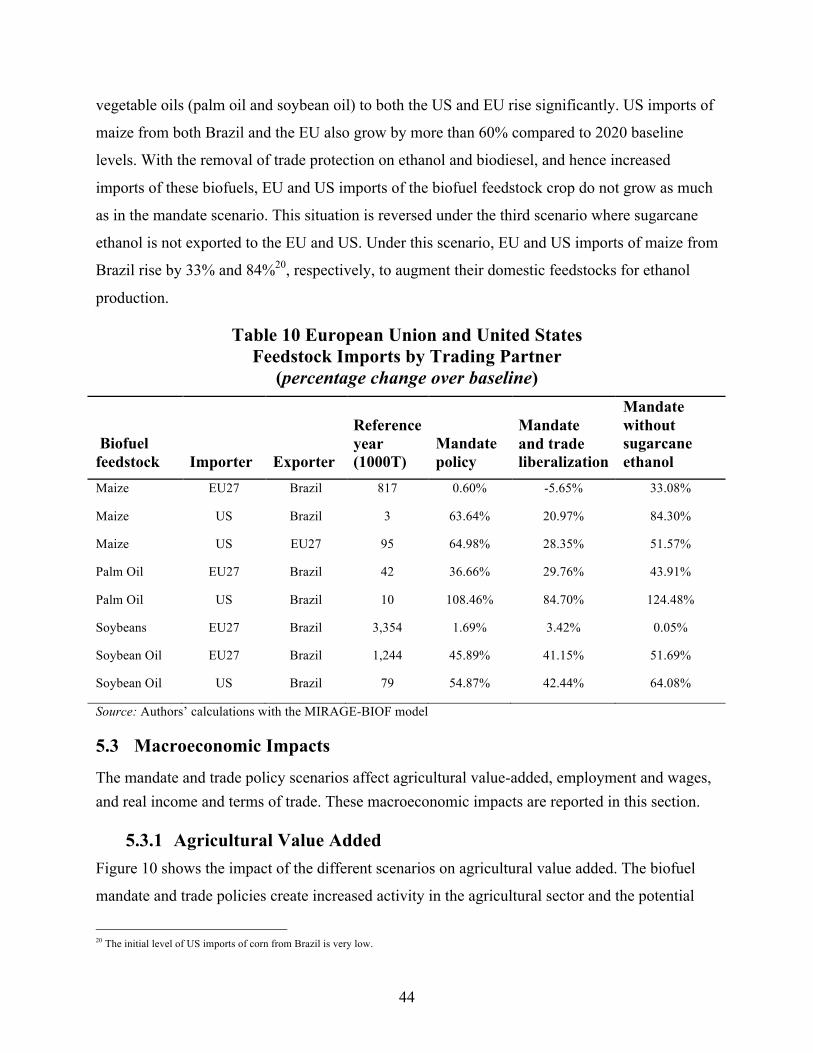
44
vegetable oils (palm oil and soybean oil) to both the US and EU rise significantly. US imports of
maize from both Brazil and the EU also grow by more than 60% compared to 2020 baseline
levels. With the removal of trade protection on ethanol and biodiesel, and hence increased
imports of these biofuels, EU and US imports of the biofuel feedstock crop do not grow as much
as in the mandate scenario. This situation is reversed under the third scenario where sugarcane
ethanol is not exported to the EU and US. Under this scenario, EU and US imports of maize from
Brazil rise by 33% and 84%20, respectively, to augment their domestic feedstocks for ethanol
production.
Table 10 European Union and United States Feedstock Imports by Trading Partner
(percentage change over baseline)
Biofuel feedstock Importer Exporter
Reference year (1000T)
Mandate policy
Mandate and trade liberalization
Mandate without sugarcane ethanol
Maize EU27 Brazil 817 0.60% -5.65% 33.08%
Maize US Brazil 3 63.64% 20.97% 84.30%
Maize US EU27 95 64.98% 28.35% 51.57%
Palm Oil EU27 Brazil 42 36.66% 29.76% 43.91%
Palm Oil US Brazil 10 108.46% 84.70% 124.48%
Soybeans EU27 Brazil 3,354 1.69% 3.42% 0.05%
Soybean Oil EU27 Brazil 1,244 45.89% 41.15% 51.69%
Soybean Oil US Brazil 79 54.87% 42.44% 64.08%
Source: Authors’ calculations with the MIRAGE-BIOF model
5.3 Macroeconomic Impacts
The mandate and trade policy scenarios affect agricultural value-added, employment and wages, and real income and terms of trade. These macroeconomic impacts are reported in this section.
5.3.1 Agricultural Value Added Figure 10 shows the impact of the different scenarios on agricultural value added. The biofuel
mandate and trade policies create increased activity in the agricultural sector and the potential
20 The initial level of US imports of corn from Brazil is very low.

45
impact on agricultural value added is positive in almost all countries/regions throughout the
world, and particularly for Brazil, the EU, and the US. It will increase by more than 1% at the
world level with peaks at 4% in Brazil under trade liberalization and 3% in the US when
sugarcane ethanol imports are restricted. Consistent with the results regarding feedstock crop
production, the mandate will boost agriculture production in all three countries but trade
liberalization will further enhance agricultural value added in Brazil, while also slowing down
growth in agricultural value added in the EU and the US. This result is reversed when the EU
and US markets are closed to sugarcane ethanol imports. Since increased domestic production of
feedstock crops will be required to replace sugarcane ethanol imports to reach the mandate, the
expansion of agricultural value added in the EU and US is greatest under this scenario.
Figure 10 Agricultural Value Added, 2020
Source: Authors’ calculations with the MIRAGE-BIOF Model
5.3.2 Employment
The impacts of the mandate on value added in Brazil can be examined more closely in terms of changes in employment of unskilled labor in the different agricultural sectors.
Table 11 shows that the US and EU mandates will increase employment in feedstock crop production in sectors related to ethanol and biodiesel production, such as maize, sugarcane, palm fruit and oil, rapeseed and rapeseed oil, soybeans and soybean oil, sunflower seeds and oil, and ethanol. Employment in sectors such as rice, sugar, meat and dairy, and other oilseeds (not used for biodiesel) will decline. With trade liberalization in ethanol exports to the EU and US, faster growth in employment occurs in the sugarcane and ethanol sectors in Brazil at the expense of employment growth in most agricultural sectors, which either decline or grow more slowly than in the mandate scenario. Under the third scenario, employment in the Brazilian sugarcane and
0%
1%
2%
3%
4%
Brazil European Union United States World
% C
hang
e ov
er B
asel
ine
Mandate
Mandate and Trade Liberalization
Mandate without Sugarcane Ethanol

46
ethanol sectors decline, while employment in the biodiesel feedstock sectors and maize sector expand.
Table 11 Unskilled Labor in Brazil (Selected Sectors) (percentage change over baseline)
Agricultural sector Mandate
Mandate and trade liberalization
Mandate without sugarcane ethanol
Maize 1.03% -3.87% 5.31%
Meat and dairy -0.62% -0.85% -0.26%
Other oil seeds -2.76% -5.75% 0.25%
Palm fruit 11.36% 7.67% 14.80%
Palm oil 12.60% 10.32% 14.67%
Rapeseed 5.41% 4.14% 6.83%
Rice -1.48% -2.62% -0.29%
Rapeseed oil 4.99% 4.44% 5.36%
Soybeans 0.48% -0.77% 2.04%
Soybean oil 2.50% 2.00% 2.93%
Sugar -6.42% -14.63% -0.15%
Sugarcane 13.73% 29.29% -1.86%
Sunflower Seed 4.41% 2.94% 6.00%
Sunflower oil 6.24% 6.24% 6.40%
Wheat -2.54% -4.46% 0.27%
Ethanol (sugar cane) 20.52% 43.94% -1.75%
Source: Authors’ calculations with the MIRAGE-BIOF model
The changes in real wages of skilled and unskilled labor, in the agricultural and non-agricultural sector, are shown in Table 12. It is the unskilled agricultural labor in the US, EU and Brazil that receives the benefit of increased wages under the mandate policy. Wages of unskilled agricultural labor in Brazil rise by 1.9% with the mandate policy and will see an even larger increase, 3.4%, when the mandate is combined with trade liberalization. Under this scenario, skilled labor and unskilled labor in the non-agricultural sectors in Brazil will face wage declines as the expansion of sugarcane and ethanol production leads to stronger demand for unskilled

47
agricultural labor. It should be noted, however, that our results may overestimate the demand for unskilled agricultural labor in 2020, since the model assumes average current technology and does not consider the technological shift with the ongoing increased mechanization in this sector, especially in regions where greater sugarcane expansion is taking place.
Table 12 Real Wages (Skilled and Unskilled) (percentage change over baseline)
Region Labor category
Reference level year 2020 Mandate
Mandate and trade liberalization
Mandate without sugarcane ethanol
Brazil Skilled 1.47 0.15% -0.01% 0.11%
Brazil Unskilled -Agri 1.32 1.90% 3.47% 0.34%
Brazil Unskilled - NonAgri 1.31 0.02% -0.11% 0.04%
Brazil Unskilled – Total 1.31 0.15% 0.14% 0.06%
EU27 Skilled 1.48 0.06% 0.06% 0.02%
EU27 Unskilled -Agri 1.24 0.23% 0.20% 0.30%
EU27 Unskilled - NonAgri 1.34 0.05% 0.05% 0.02%
EU27 Unskilled – Total 1.33 0.06% 0.05% 0.03%
US Skilled 1.32 0.07% 0.07% 0.03%
US Unskilled -Agri 1.05 0.24% 0.20% 0.24%
US Unskilled - NonAgri 1.21 0.08% 0.10% 0.04%
US Unskilled – Total 1.21 0.08% 0.11% 0.05%
Source: Authors’ calculations with the MIRAGE-BIOF model
5.3.3 Real Income Effects The real income effects of the EU and US mandates shown in Table 13 indicate that the
mandates have negative global effects, on average (-0.04% under all scenarios). As a net
agricultural exporter, Brazil is positively impacted in all cases due to increased agricultural
prices in world markets (see terms of trade effects) and increased demand for its products. The
real income effects for the US and the EU are very limited (smaller than 0.05%). Since both
countries implement distortive policies, the mandates have an efficiency cost than can be
compensated only by the terms of trade effects (evolution of the export prices vs. import prices),
the latter being driven by the fall in demand and prices of oil. Aside from these countries, oil

48
producing countries such as those in the CIS and the SSA21 region suffer losses due to reduction
of oil prices (up to -1.8%) led by the shift in demand toward biofuels, thereby reducing aggregate
world real income. However, the real behavior of oil producers to the increase of biofuels market
share is difficult to assess due to the lack of perfect competition in this sector. The price/quantity
response of a cartel of oil producers may be different from the model projections and, therefore,
the real income effects driven by the terms of trade effects have to be taken carefully.
Table 13 Real Income and Terms of Trade (percentage change over baseline)
Indicator Region
Reference year 2020 (US$ billion)
Mandate policy
Mandate and trade liberalization
Mandate without sugarcane ethanol
Real income Brazil 835 0.34% 0.42% 0.12%
Real income CAMCarib 406 0.13% 0.01% 0.01%
Real income China 4,194 0.00% 0.01% -0.01%
Real income CIS 1,030 -0.65% -0.55% -0.46%
Real income EU27 13,857 0.05% 0.03% 0.02%
Real income IndoMalay 537 0.01% 0.05% 0.08%
Real income LAC 1,491 -0.14% -0.11% -0.08%
Real income RoOECD 7,754 0.00% -0.01% -0.02%
Real income RoW 5,254 -0.42% -0.35% -0.31%
Real income SSA 863 -0.48% -0.40% -0.34%
Real income US 13,868 0.04% -0.01% 0.02%
Real income World 50,089 -0.04% -0.04% -0.04%
Terms of trade Brazil
1.36% 2.34% 0.39%
Terms of trade CAMCarib
0.51% 0.08% 0.03%
Terms of trade China
0.19% 0.17% 0.11%
Terms of trade CIS
-0.92% -0.77% -0.64%
Terms of trade EU27
0.13% 0.10% 0.10%
Terms of trade IndoMalay
0.23% 0.23% 0.23%
21 Due to existing difficulties related to a fair distribution of oil rents in many developing countries, the real income loss at the macro level may not lead to a deterioration of the situation for most of the population.

49
Indicator Region
Reference year 2020 (US$ billion)
Mandate policy
Mandate and trade liberalization
Mandate without sugarcane ethanol
Terms of trade LAC
-0.20% -0.18% -0.07%
Terms of trade RoOECD
0.09% 0.09% 0.06%
Terms of trade RoW
-0.54% -0.45% -0.39%
Terms of trade SSA
-0.85% -0.72% -0.59%
Terms of trade US
0.36% 0.21% 0.32%
Source: Authors’ calculations with the MIRAGE-BIOF Model
For the EU and the US, the best outcome is the mandate with the status quo on trade
policies; trade restrictions will lead to greater inefficiency, and more liberalization will erode the
terms of trade gains. For the US, trade liberalization leads to a deterioration of the terms of trade
that are stronger than in the EU; the starting point for the US is a large trade deficit (which
implies higher marginal real income costs of any deterioration of its real exchange rate [needed
to compensate increased imports]).
5.4 Land-use Impacts
Changes in crop production, particularly due to the increased demand for feedstock crops used as
inputs in biofuels, will have different implications on the expected patterns of land use under the
mandates and trade liberalization scenarios. Most of the environmental debate around biofuels is
now focused on changes in land use and the role of biofuel policies on agricultural expansion,
which leads to deforestation and increases in GHG emissions.
Table 14 indicates the variation in land use by type of land, which could be expected from the policy scenarios. The amount of cropland is significantly affected in Brazil (+2.7% under the mandate scenario, 3.9% with trade liberalization, and 1.7% without sugarcane ethanol – see also Figure 11). This result is due to the combination of the demand for ethanol (sugarcane) and oilseeds (soya). However, our detailed modeling of land extension and land reallocation indicates that primary forests (e.g. Amazonia) are not the main source of cropland. More than half of the land will be released by the livestock sectors (-1.8% to -2.6% of pasture), followed by savannah/grassland (e.g. Cerrado in southeastern Brazil). It is clear that our assumption about intensification of livestock production can play a critical role here and should be considered carefully. At the same time, it is also critical that ranchers pay the price of the land they use;

50
otherwise they will have no incentives to intensify production and may continue with deforestation. The other regions that are affected are the EU, CIS, LAC and Indonesia/Malaysia.
Table 14 Land Use (percentage change over baseline)
Reference year 2020 (1000 ha) Mandate
Mandate and trade liberalization
Mandate without sugarcane ethanol
Pasture Brazil 119,021 -1.84% -2.64% -1.11%
Pasture EU27 68,823 -0.02% -0.02% -0.03%
Pasture US
61,453 0.02% 0.01% 0.02%
Pasture World 1,045,634 -0.29% -0.36% -0.21%
Cerrado Brazil 183,839 -0.16% -0.24% -0.10%
Grassland EU27 20,520 -0.33% -0.27% -0.45%
Grasslnd US
282,403 -0.04% -0.03% -0.05%
Savannah/cerrado/grassland World 2,986,028 -0.04% -0.03% -0.03%
Cropland Brazil 104,851 2.69% 3.87% 1.69%
Cropland EU27 93,765 0.19% 0.16% 0.26%
Cropland US
103,735 0.23% 0.14% 0.26%
Cropland World 1,392,942 0.40% 0.44% 0.33%
Managed forest Brazil 16,925 -1.04% -1.53% -0.98%
Managed forest EU27 148,354 -0.03% -0.02% -0.04%
Managed forest US
143,542 -0.04% -0.03% -0.05%
Managed forest World 1,093,845 -0.08% -0.07% -0.08%
Primary forest Brazil 420,048 -0.02% -0.03% -0.02%
Primary forest EU27 6,780 0.00% 0.00% 0.00%
Primary forest US
161,001
Primary forest World 2,669,467 -0.01% -0.01% -0.01%
Source: Authors’ calculations with MIRAGE-Biof Model

51
Figure 11 Agricultural Land Extension MHa, 2020
Source: Authors’ calculations with the MIRAGE-BIOF Model
5.5 Greenhouse Gas Emissions
GHG emissions balance accounts for direct emissions savings in the biofuel production cycle
and the emissions associated with changes in land use22. As shown in Figure 12, the sum of
direct emissions reductions23 generated by the substitution of fossil fuel by biofuels and implied
by the mandate at -74 million tons of CO2 equivalent in 2020 is slightly less than the sum of
direct emissions when liberalization of trade in ethanol and biodiesel is combined with the
mandate: -81 million tons of CO2 equivalent in 2020. Direct emissions reductions are
significantly less (-41 mtCO2eq) when sugarcane ethanol is eliminated. This result is driven by
the efficiency of sugarcane ethanol. The net emissions balance (land use emissions minus direct
emission savings) is positive and slightly larger under the liberalization case (-41 mtCO2eq) than
under the pure mandate scenario (-32 mtCO2eq). Even if the liberalization leads to more
emissions through indirect land-use effects, using efficient imported biofuels delivers a net
missions reduction in a 20-year period. However, when sugarcane ethanol is not allowed in the
mandate, the direct emissions savings are cancelled out by land-use emissions at the world level.
22 The GHG emissions from fertilizers and intensification are not captured in this analysis. 23 Each MJ of fossil fuel is assumed to generate 25gr. of carbon, i.e. about 92 gr. of CO2.
0.00 1.00 2.00 3.00 4.00 5.00 6.00 7.00
Man
date
Man
date
and
Tr
ade
Libe
raliz
atio
n
Man
date
w
ithou
t Su
garc
ane
Etha
nol
Brazil Central America and Caribbean Countries China Commonwealth of Independent States European Union Indonesia and Malaysia Latin American Countries (inc. Argentina) Rest of OECD (inc. Canada & Australia)

52
Under this scenario, the decline in sugarcane production in Brazil and the increased demand for
feedstock crops for biofuels and food in the EU and US encourages increased production of less
environmentally efficient crops (oilseeds for biodiesel, maize) in Brazil.
These results indicate that the biofuel mandates can lead to positive net GHG emissions
reductions24, but further reductions can be achieved when the trade barriers are removed along
with the mandate.
Figure 12 Emissions Balance, 2020 (MTCO2eq)
Source: Authors’ Calculations using the MIRAGE-BIOF Model
Note: The emissions credit is attributed to the country that consumes the biofuel. Land-use change emissions are attributed to the region where the expansion took place.
Table 15 displays the carbon balance sheet of the EU and US mandates and the trade policy scenarios. The upper part of the table displays the total carbon release (from forest biomass and soil contents) due to the change in land use from 2008-2020 following the implementation of the mandate. The lower part shows average land-use change effect computed with our model, which is equal to the sum of carbon release from forest biomass and soil carbon content. All annual coefficients take the stock value of the upper table and divide them by 20 years. This is then divided by the increase in EU consumption of biofuels. The results indicate a reduction in GHG emissions under the US and EU mandates, with the net emission balance over a 20-year period of about -20.8gCO2/MJ under the US and EU mandates, and -28gCO2/MJ if the mandates are not associated with an open trade policy. However, the GHG emissions balance
24 This does not consider the effects of fertilizers.
-100
-80
-60
-40
-20
0
20
40
60
Brazil EU27 USA World Brazil EU27 USA World Brazil EU27 USA World
% C
hang
e ov
er B
asel
ine
Land use change
Direct cycle
Mandate Mandate and Trade Liberalization
Mandate without Sugarcane Ethanol

53
turns positive at +7.9 gCO2/MJ when sugarcane ethanol imports are not allowed in the mandate. These coefficients are average values since they are based on the full mandate increase in both EU and US and take into consideration all the direct and indirect effects in the CGE framework in terms of income and substitution effects. CO2 variations, which are not directly related to biofuel policies (such as the income effects on the steel industry), are excluded.
Table 15 Carbon Balance over a 20-Year Period
Mandate
Mandate and trade liberalization
Mandate without sugarcane ethanol
Total carbon release from forest biomass (MtCO2eq) 268.28 231.17 283.26
Total carbon release from carbon in soil (MtCO2eq) 576.95 570.69 535.16
Marginal carbon reimbursement rate (MtCO2 per year) -74.27 -81.37 -40.55
Carbon debt payback time (years) 11.38 9.85 20.18
EU+US Consumption of biofuel in 2020 (million GJ) 2502 2524 2069
Annual carbon release from forest biomass (gCO2eq/MJ) 15.64 13.69 24.89
Annual carbon release from below ground (gCO2eq/MJ) 23.16 22.51 32.92
Annual direct savings (gCO2/MJ) -59.63 -64.19 -49.89
Total emission balance over a 20-year period (gCO2/MJ) -20.83 -27.98 7.92
Source: Authors’ Calculations with the MIRAGE-BIOF Model
6 Concluding Remarks
This study shows that the incremental expansion of the biofuel consumption under the US and
EU biofuel mandates will be beneficial at the global level in terms of value addition in the
agricultural sector, in the expansion of global trade, and in the reduction of GHG emissions. The
biofuel mandates will have limited impacts on real food prices. However, there will also be
global costs driven mainly by the decline in income of oil exporting countries. Since both the US and EU mandates favor greater ethanol consumption, it is the ethanol
sector that will expand more compared to biodiesel. Brazil will benefit from increased
production and exports of sugarcane ethanol to supply these markets, especially when the EU
and US biofuel mandates are combined with trade liberalization in biofuels in both countries
since higher ethanol production and exports will be accompanied by higher real income gains
and agricultural value added. Use of cropland in Brazil will increase, with land coming mostly

54
from pasture. Unilateral biofuel trade liberalization will dampen the positive economic impacts
of the mandate for the EU and the US but will enhance the reduction of GHG emissions as these
countries increase imports of the more environmentally efficient sugarcane ethanol.
Although Brazil will still experience real income gains when the US and the EU
discontinue their use of imports of sugarcane ethanol, the gains will be sharply lower. However,
Brazil will be able to tap other markets for ethanol while also allowing production and exports of
other agricultural sectors (e.g. oilseeds and vegetable oils for biodiesel production) to expand.
The exclusion of sugarcane ethanol imports will require a significant expansion of domestic
ethanol production in the US and the EU. Production of feedstock crops, and thus cropland use,
will also increase in these countries. Although more beneficial for the agricultural sector and for
real income in these countries, the mandate policy without sugarcane ethanol has more adverse
implications for the environment in terms of positive net CO2 emissions.
This study indicates that the US and EU biofuel mandates have generally beneficial
impacts on the agricultural markets and on the environment in terms of reduced CO2 emissions.
These benefits are further enhanced if the mandate policy is accompanied by liberalization in
biofuels trade. Trade liberalization will bring greater benefits to consumers in terms of lower fuel
prices and greater reductions in CO2 emissions, when sugarcane ethanol is traded. While it will
result in important adjustments in the agricultural sector, it will generally be beneficial for the
agriculture sector and farm producers.

55
Annex I Additional Results
Table 16 Biofuel Consumption (percentage change over baseline)
Biofuel Region
Reference year 2020 (Mtoe) Mandate
Mandate with trade liberalization
Mandate without sugarcane ethanol
Biodiesel Brazil 4.21 -0.16% -0.07% -0.23%
Biodiesel China 0.18 -3.63% -4.70% -3.07%
Biodiesel EU27 9.10 45.41% 45.59% 44.92%
Biodiesel IndoMalay 3.78 0.68% 0.58% 0.50%
Biodiesel LAC 0.48 -16.83% -15.69% -16.12%
Biodiesel US 1.25 151.66% 154.85% 143.89%
Biodiesel World 26.17 22.37% 22.36% 21.36%
Ethanol Brazil 34.90 -4.61% -7.74% -0.83%
Ethanol CAMCarib 1.28 136.73% -18.22% -46.13%
Ethanol China 14.81 0.68% 0.58% 0.45%
Ethanol EU27 1.87 250.32% 250.74% 249.13%
Ethanol LAC 0.75 -6.68% -1.19% 0.20%
Ethanol US 17.80 107.07% 109.70% 49.90%
Ethanol World 98.81 24.29% 21.72% 13.08%
Source: Authors’ Calculations using the MIRAGE-BIOF Model

56
Table 17 European Union Biofuel Imports by Partner (percentage change over baseline)
Biofuel Region
Reference year 2020 (Mtoe) Mandate
Mandate with trade
liberalization
Mandate without
sugarcane ethanol
Biodiesel Brazil 0.00 57.12% 50.70% 63.34% Biodiesel China 0.00 79.16% 78.99% 79.46% Biodiesel IndoMalay 0.30 86.08% 84.86% 86.13% Biodiesel LAC 0.87 41.37% 42.82% 39.78% Biodiesel RoOECD 0.00 84.88% 189.35% 88.28% Biodiesel US 0.00 10.44% 13.90% 73.84% Biodiesel World 1.18 52.86% 53.82% 51.80% Ethanol Brazil 0.98 416.65% 491.49% -99.99% Ethanol CAMCarib 0.06 298.02% -99.11% -100.00% Ethanol US 0.01 121.46% 5217.11% 12581.97% Ethanol World 1.05 407.43% 490.40% -8.22%
Source: Authors’ Calculations with the MIRAGE-BIOF Model
Table 18 Biofuel Blending Rates
Biofuel Region
2008 blending rate
2020 blending rate
Mandate
Mandate and trade liberalization
Mandate without sugarcane ethanol
Biodiesel Brazil 1.5% 6.1% 6.1% 6.1% 6.1% Biodiesel EU27 2.7% 2.7% 4.0% 4.0% 4.0% Biodiesel US 0.1% 0.4% 1.0% 1.0% 1.0%
Ethanol Brazil 40.2% 52.3% 49.9% 48.4% 51.8% Ethanol EU27 0.6% 0.6% 2.0% 2.0% 2.0% Ethanol US 5.1% 6.0% 12.2% 12.2% 8.9%
All biofuels Brazil 41.7% 58.5% 56.0% 54.5% 57.9% All biofuels EU27 3.3% 3.3% 6.0% 6.0% 6.0% All biofuels US 5.2% 6.4% 13.2% 13.2% 9.8%
Source: Authors’ Calculations with the MIRAGE-BIOF Model Note: Figures in this table are additive: the mandate on a single fuel is reported for the quantity of total fuel (gasoline + diesel + biofuel).

57
Table 19 Intensification Index for Cultivation (percentage change over baseline)
Mandate Mandate
with trade
Mandate without
sugarcane ethanol
Maize Brazil 2.60% -1.48% 6.40% Maize EU27 1.37% 0.46% 2.42% Maize US 3.43% 1.47% 4.34% Other crop Brazil -1.97% -3.96% 0.00% Other crop EU27 0.47% 0.64% 0.28% Other crop US -0.04% 0.14% -0.07% Other oilseeds Brazil -1.63% -4.43% 0.94% Other oilseeds EU27 0.30% 0.60% -0.07% Other oilseeds US 0.04% 0.37% -0.29% Palm fruit Brazil 13.50% 10.87% 15.93% Palm oil Brazil 14.97% 11.62% 18.14% Rapeseed Brazil 7.07% 6.80% 7.55% Rapeseed EU27 4.46% 4.62% 3.80% Rapeseed US 1.83% 2.24% 1.53% Rice Brazil -0.19% -0.45% 0.02% Rice EU27 0.01% 0.01% 0.05% Rice US -0.23% -0.16% -0.26% Soybeans Brazil 1.91% 1.59% 2.47% Soybeans EU27 0.54% 0.99% -0.29% Soybeans US -0.23% 0.55% -0.71% Sugar beet or cane Brazil 28.30% 61.69% -2.12% Sugar beet or cane EU27 40.55% 5.07% 90.39% Sugar beet or cane US 2.15% 0.00% -0.15% Sunflower Brazil 6.00% 5.48% 6.69% Sunflower EU27 3.72% 3.79% 3.14% Sunflower USA 2.09% 2.32% 1.79% Sunflower oil Brazil 7.20% 6.36% 8.09% Sunflower oil EU27 7.05% 7.04% 6.35% Sunflower oil US 2.11% 2.99% 0.96% Vegetable and fruits Brazil -1.01% -1.81% -0.30% Vegetable and fruits EU27 0.14% 0.11% 0.10% Vegetable and fruits US 0.70% 0.34% 0.83% Wheat Brazil -1.00% -2.08% 0.86% Wheat EU27 -0.23% -0.43% 0.38% Wheat US -0.53% -0.42% -0.40%
Source: Authors’ Calculations with the MIRAGE-BIOF Model

58
Table 20 GDP and Welfare (percentage change over baseline)
Indicator Region
Reference year 2008 (US$ billion)
Reference year 2020 (US$ billion) Mandate
Mandate with trade
Mandate without sugarcane ethanol
GDP Brazil 617 888 -0.03% -0.29% 0.06% GDP Caribbean 266 375 -0.01% 0.01% 0.03% GDP China 1,769 4,380 -0.04% -0.03% -0.04% GDP CIS 805 1,136 -0.02% -0.02% -0.03% GDP EU27 11,536 13,761 0.02% 0.02% 0.00% GDP IndoMalay 391 635 -0.01% -0.02% 0.01% GDP LAC 1,125 1,537 0.00% 0.01% -0.01% GDP RoOECD 6,629 8,115 0.01% 0.01% 0.00% GDP RoW 3,353 5,417 0.02% 0.02% -0.01% GDP SSA 562 877 -0.06% -0.05% -0.06% GDP US 10,609 12,980 0.01% 0.03% -0.02% GDP World 37,662 50,101 0.01% 0.01% -0.01% Welfare Brazil 578 835 0.34% 0.42% 0.12% Welfare CAMCarib 288 406 0.13% 0.01% 0.01% Welfare China 1,630 4,194 0.00% 0.01% -0.01% Welfare CIS 726 1,030 -0.65% -0.55% -0.46% Welfare EU27 11,607 13,857 0.05% 0.03% 0.02% Welfare IndoMalay 321 537 0.01% 0.05% 0.08% Welfare LAC 1,091 1,491 -0.14% -0.11% -0.08% Welfare RoOECD 6,363 7,754 0.00% -0.01% -0.02% Welfare RoW 3,231 5,254 -0.42% -0.35% -0.31% Welfare SSA 551 863 -0.48% -0.40% -0.34% Welfare US 11,269 13,868 0.04% -0.01% 0.02% Welfare World 37,655 50,089 -0.04% -0.04% -0.04%
Source: Authors’ Calculations with the MIRAGE-BIOF Model

59
Annex II Price Changes in Partial and General Equilibrium Models
In the absence of modeled linkages to the rest of the economy, partial equilibrium models
(PEMs) tend to overestimate the effect of exogenous shocks on prices and other indicators in
their system. There are several PEMs25 that have been developed and used to explore, and
analyze, the implications of various policy mandates. These PEMs focus on the agricultural
sector and its policies and attempt to provide policy implications at the country, regional and
even global level.
The sectoral structure in these models is highly detailed and allows one to focus on the
most recent international interest, mostly recently the global biofuel debate. In trying to address
country-level and/or global-policy analysis by using PEMs, other individual modules have to be
linked to a central PEM26. Despite the extensive level of detail PEMs provide to the sector under
study, they do not link that sector of study to the other markets/sectors such as the product, factor
and global markets in the system. Factor markets in particular, play a critical role in the long-
term adjustments to any shock, for instance, land can be extended or improved through
investment and labor will flow to expanding markets thus raising productivity. Most of these
mechanisms are endogenous to the economy and PEMs cannot capture them. As a result, the link
between policy choices and economic outcomes is not as comprehensive or as encompassing as
it would be in a CGE model.
Typically in PEMs, the results show higher magnitudes for the variables of focus. As an
example, in an agricultural sector PEM, a mandate targeting increased blending ratios of ethanol
with gasoline is considered an exogenous shock and would ultimately increase the demand for
feedstock and other crops. The result would be an increase in the price, and supply, of biofuel
feedstock, other substitute agricultural crops and activities. In this PEM, the multiplier (direct)
effects of such a shock may be concentrated in one sector and are only fed exogenously to the
remaining modules to calculate values for indicators of interest. The lack of this intersectoral link
25 Most notable PE models in the recent literature are; CAPRI (Britz and Wetzel, 2008), AGLINK/COSIMO (OECD, 2007), FAPRI and IMPACT (Rosegrant et al, 2008). 26 For example, the demand module(s) in CAPRI feed commodity prices to its supply module in order to determine supplier decisions, (Britz and Witzle, 2008) and the IMPACT model is fed water use data by crop and region from a water module (Rosegrant et al, 2008).

60
and its ensuing iterative process of feeding back and forth within and amongst sectors in the
economy leads to results with higher magnitudes than those obtained by CGE models27.
Once an individual sector is linked to the rest of the economy, as is the case in a CGE
model, not only do the direct effects of this exogenous shock leak or transfer to the other sectors
and agents in the modeled economy, but also indirect effects also take place to add another layer
of analysis to the results. For instance, given the same exogenous shock mentioned above of a
biofuel mandate, the resultant increase in feedstock, and other crop supply and prices, may have
other sectoral implications outside the agricultural sector.
In a CGE model that models a country that produces ethanol from sugarcane, such a
biofuel mandate would lead to an increase in the supply and price of sugarcane. Sugarcane is
also an input for sugar, which is a food product and is also a feedstock for producing ethanol. In
the case of sugar for food, the increase in the price of sugarcane, may have various effects on the
demand for sugarcane in the food processing industry. Assuming that the price elasticity of
demand for sugarcane in the food processing sector does not exactly offset the price elasticity of
sugar supply in the same sector, ceteris paribus, the demand for sugarcane (to produce sugar for
consumption) will change. Depending on the magnitude of this change, there will be back and
forth effects on factor allocations, and consequently, factor income allocations, incomes of
sugarcane farmers (and other farmers in the system), the sugar producing industry, other sectors
in the economy, the consumption of sugar (and thus the consumption and saving decisions of the
households), the saving investment balance, the trade balance, the current account balance and
finally GDP. However, the process continues by feeding back into the agricultural sector and out
again until eventually the system reaches an equilibrium in all its variables.
The increase in the price of sugarcane (and consequently in the price of sugar), in the
absence of any support policies for fuel ethanol production, and in the absence of any subsidies
on its consumer price and depending on the price of oil, this price increase may lead to an
increase in the price of fuel ethanol. In short, the impacts of such a biofuel mandate would not
stop with the impacts only on one sector, as in a PEM, in a CGE model the ripple effects of this
biofuel mandate (or an exogenous shock) would keep circulating and expanding to include more
27 The extent of the price, demand and supply responsiveness would depend on the price elasticities as well as the production function(s) assumed for the sector.

61
sectors and agents so that there are more macro indicators affected, albeit with less magnitude
than the typical PEM.
Based on the absence of their intersectoral linkages, PEMs that have analyzed the recent
commodity price hikes may not have appropriately reflected the longer-term price trends as
previously expected. In the recent literature, there is a renewed debate about a new plateau that
now exists for commodity prices after the recent commodity price increase. The movement of
commodity prices are a function of several factors, both supply side and demand side that, if they
coincide, may bring about the “perfect storm” that led to the 2007/2008 commodity price hikes
(Trostle 2008 and Hertel, 2010). The literature states that commodity price variability
overwhelms price trends (Baffes and Haniotis, 2010) and that it is difficult to predict future
trends based on historic trends alone. Model structure, assumptions used, the time period under
study, country-specific stylized factors and global links all contribute to determining commodity
price trends and forecasts. Furthermore, commodity markets should not be analyzed in isolation
from one another nor from the rest of the economy as they are strongly interlinked through their
substitutability and/or complementarity. A CGE model of the biofuel sector would analyze the
commodity markets au lieu of the recent biofuel mandates and as such would, given the
intersectoral linkages, give rise to results that are more moderate and more realistic in the longer
term, than a PEM.

62
References
Al-Riffai, P., B. Dimaranan, and D. Laborde. 2010. Global Trade and Environmental Impact
Study of the EU Biofuels Mandate. Final Draft Report Submitted to the Directorate
General for Trade, European Commission. Available at:
http://www.ifpri.cgiar.org/sites/default/files/publications/biofuelsreportec.pdf.
Baffes, John and Tassos Haniotis. 2010. “Placing the 2006/08 Commodity Price Boom into
Perspective.” World Bank Policy Research Working Paper # 5371. Washington D.C. July
2010.
Barr, K.J., B.A. Babcock, M. Carriquiry, A. Nasser, L. Harfuch. 2010. “Agricultural Land
Elasticities in the United States and Brazil.” Center for Agriculture and Rural
Development Working Paper 10-WP 505.
Bchir, H., Y. Decreux, J-L Guerin, and S. Jean. 2002. "MIRAGE, a Computable General
Equilibrium Model for Trade Policy Analysis," CEPII Working Paper No 2002-17.
France. December 2002. Available at:
http://www.cepii.fr/anglaisgraph/workpap/pdf/2002/wp02-17.pdf
Bouët, A., B. Dimaranan, & H. Valin. 2010. Modeling the Global Trade and Environmental
Impacts of Biofuels Policies, IFPRI Discussion Paper 01018, August 2010.
Bouët, A., L. Curran, Dimaranan, B., Ramos, M.P., and H. Valin. 2008. “Biofuels: Global Trade
and Environmental Impact Study”. Report for DG Trade. ATLASS Consortium.
Britz, W. and Witzke, P. (eds.). 2008. CAPRI Model Documentation 2008: Version 2. Available
at: http://www.capri-model.org/docs/capri_documentation.pdf (accessed 17 September
2010).
Burniaux, J. M. and T.P. Truong. 2002. "GTAP-E: An Energy-Environment Version of the
GTAP Model," GTAP Technical Paper No 16, Center for Global Trade Analysis, Purdue
University, West Lafayette, IN.
Commission of the European Communities (CEC). 2006. Renewable Energy Roadmap.
COM(2006) 848, Commission of the European Communities, Brussels.

63
Commission of the European Communities (CEC). 2008. Proposal for a Directive of the
European Parliament and of the Council on the Promotion of the Use of Energy from
Renewable Sources. Commission of the European Communities, Brussels.
Decreux, Y. and H. Valin. 2007. MIRAGE : Updated Version of the Model for Trade Policy
Analysis: Focus on Agriculture and Dynamics. CEPII Working Paper, N°2007-
15, October 2007. [Online] Available at:
http://www.cepii.fr/anglaisgraph/workpap/pdf/2007/wp07-15.pdf.
Edwards, R. 2010. "What do we know about Peatland Drainage Emissions?" European
Commission, Joint Research Centre.
Environmental Protection Agency. 2009. “Draft Regulatory Impact Analysis: Changes to
Renewable Fuel Standard Program.”
European Council. 2009. “Directive 2009/30/Ec of the European Parliament and of The
Council.” 23 April 2009. Available at: http://www.r-e-a.net/document-
library/thirdparty/rea-and-fqd-documents/FQD_090605_Directive_200930EC_OJ.pdf
Food and Agricultural Policy Research Institute (FAPRI). Available at:
http://www.fapri.org/models/
Hertel, Thomas 2010. “The Global Supply and Demand for Agricultural Land in 2050: A Perfect
Storm in the Making?” AAEA Presidential Address, July 26, 2010. US.
Horridge, J.M. 2005. SplitCom: “Programs to Disaggregate a GTAP Sector.” Centre of Policy
Studies, Monash University, Melbourne, Australia. Available at:
http://www.monash.edu.au/policy/SplitCom.htm
International Energy Agency. 2009. “World Energy Outlook – 2009.”
Kampman, B, F. Brouwer and B. Schepers. 2008. “Agricultural Land Availability and Demand
In 2020, Report to the Renewable Fuels Agency.” published on
www.renewablefuelsagency.org, CE Delft, elft, The Netherlands.
Ludena, C., T. Hertel, P. Preckel, K. Foster, and A. Nin Pratt. 2006. ‘Productivity Growth and
Convergence in Crop, Ruminant and Non-Ruminant Production: Measurement and

64
Forecasts.’ GTAP Working Paper No. 35. Available at:
https://www.gtap.agecon.purdue.edu/resources/download/2900.pdf.
Ludena, C. 2010. "Agricultural Productivity Growth, Efficiency Change and Technical Progress
in Latin America and the Caribbean." IDB Working Paper Series No.IDB-WP-186.
Available at: http://www.iadb.org/res/publications/pubfiles/pubIDB-WP-186.pdf
Narayanan G., B. and T. L. Walmsley, Eds. 2008. Global Trade, Assistance and Protection: The
GTAP 7 Database. Center for Global Trade Analysis, Purdue University. Available at:
https://www.gtap.agecon.purdue.edu/databases/v7/v7_doco.asp
OECD. 2007. Documentation of the AgLink-CosimoModel. Paris: Organisation for Economic
Co–operation and Development.
Okagawa, A. and K. Ban. 2008. "Estimation of Substitution Elasticities for CGE Models,"
Discussion Papers in Economics and Business from Osaka University No 08-16,
Graduate School of Economics and Osaka School of International Public Policy (OSIPP).
Rosegrant, M., C. Ringler, S. Msangi, T. Sulser, T. Zhu and S. Cline. 2008. “International Model
for Policy Analysis of Agricultural Commodities and Trade (IMPACT): Model
Description.” International Food Policy Research Institute, Washington DC, June 2008.
Seale, J., A. Regmi, and J.A. Bernstein. 2003. “International Evidence on Food Consumption
Patterns.” Technical Bulletin No. TB1904.
Taheripour, F., D.K. Birur, T.W. Hertel, and W.E. Tyner. 2008. “Biofuels and Their By-
Products: Global Economic and Environmental Implications.” GTAP Conference paper,
Helsinki, June 2008.
UNICA. 2010. “Brazilian Ethanol Projection.” Memorandum. Brazilian Sugarcane Industry
Association. Available at:
http://sweeteralternative.com/blog/MemoBrazilianEthanolProjections.pdf.
Valin, H., B. Dimaranan, and A. Bouët. 2009. "Biofuels in the World Markets: A Computable
General Equilibrium Assessment of Environmental Costs Related to Land-use changes,"
CATT Working Paper No. 6, November.