EUROTOX2013-CEC5:Statist. Evaluation in Toxicology

Topic I: Statistical principles andanalysis of repeated toxicity studies

Ludwig A. Hothornhothorn@biostat.uni-hannover.de

August 12, 20131 / 86

Aims for the next hour I

- Evaluation strategies of repeated (short-term, 28 days...6 months)toxicological studies

- Using confidence intervals instead of common-used p-values

- Using two-sample confidence intervals for a proof of hazardwithout FWER-control

- Using Dunnett/Williams procedures: parametric (incl. varianceheterogeneity), non-parametric, proportions with FWER-control(again proof of hazard) according to NTP recommendations

- Using R - real data example based exercises

- And, next unit: analysis of mutagenicity assays, namely i) counts, ii)k-fold rule, iii) muta-tox-problem, iv) ...

- And, final unit: proof of safety, namely significant toxicity approach

2 / 86

Motivating examples I

- Example I: Continuous endpoints

I The data of a 13 weeks feeding study on Sodium dichromate dihydratein F344 Rats was downloaded from US-NTP

I For each sex 10 rats were randomized to control, 62.5, 125, 250, 500and 1000 mg/kg.

I Several hematological and clinical chemistry endpoints were measuredafter 5, 23 and 93 days of administration; here organ weight (liver) data

n=10 n=10 n=10 n=10 n=10 n=10

8

10

12

0 62.5 125 250 500 1000dose

Live

rWt

3 / 86

Motivating examples III These data are almost representative for short-term studies: both

sexes, 10 animals/group, many endpoints. However, three instead fivedose groups are common and only one final measurement, whereassometimes a baseline measure is available.

- Example II: Histopathological findingsIncidence data: incidences of tubular epithelia hyaline dropletdegeneration in male rats were reported for a 28-day oral dose toxicitystudy of nonylphenol to: 0/10, 0/10, 3/10, 8/10 [WSI+07].

- Example III: Graded findingsNon-Neoplastic lesions in the P-Cresidine carcinogenicity study oneach 30 male mice: 1) hyperplasia in parotid gland (salivary glands)and 2) kidney hydoephoris (where the single finding minimal wascategorized as none finding as the unlisted animals) The secondexample shows no finding in the control at all.

- Data files in .cvs format available

4 / 86

Motivating examples III

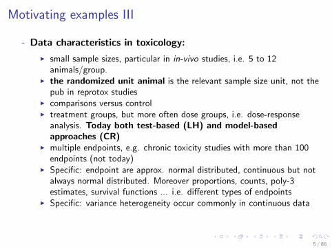
- Data characteristics in toxicology:

I small sample sizes, particular in in-vivo studies, i.e. 5 to 12animals/group.

I the randomized unit animal is the relevant sample size unit, not thepub in reprotox studies

I comparisons versus controlI treatment groups, but more often dose groups, i.e. dose-response

analysis. Today both test-based (LH) and model-basedapproaches (CR)

I multiple endpoints, e.g. chronic toxicity studies with more than 100endpoints (not today)

I Specific: endpoint are approx. normal distributed, continuous but notalways normal distributed. Moreover proportions, counts, poly-3estimates, survival functions ... i.e. different types of endpoints

I Specific: variance heterogeneity occur commonly in continuous data

5 / 86

Proof of hazard I

- Design: (negative) control, k doses (rare, but appropriate: positivecontrol)

- Example: exa1 (liver weighs)

n=10 n=10 n=10 n=10 n=10 n=10

8

10

12

0 62.5 125 250 500 1000dose

Live

rWt

- The exptl. question: which dose is significantly changed with respectto control (or sign. reduced- notice one-sided testing)

6 / 86

Proof of hazard II- First: naive two-sample test: [0, 500]

- Problem 1: for the common small sample sizes, no meaningful teston gaussian distribution, or not (and variance homogeneity, orheterogeneity) exists

- Recommendation 1:

i trusting the robustness of t-test (and related tests) orii using non-parametric tests or

iii modeling the distribution (e.g. quasi-Poisson)

- Using common t-test: p-value 0.0014

- Q.: Can we conclude a significant weight reduction, although thet-test was 2-sided. yes, we can (explain it)

- Look on boxplot: a serious variance heterogeneity occur (a ”good”one ... SD500 < SD0.

- Problem 2: t-test is not robust against variance heterogeneity,particularly when nC >>,<< nD

7 / 86

Proof of hazard III- Use the Welch-t-test instead p: 0.0027. Realize the bias of

common t-test!

- No powerful test on variance heterogeneity for small ni exists,therefore Recommendation 2: Use always the Welch-t-test (onlyminor power loss for homogeneous variances)

- Problem 3: Is the non-parametric Wilcoxon-test appropriate, e.g.when data are skewed (see 1000µg in the boxplot), or outlier occur?Counter-facts:

1 WMW does not test mean differences (even not median differences); it testsstochastic order- hard to interpret (but see xxx)

2 WMW is NOT robust against heterogeneous variances. Recently, aBehrens-Fisher modification is available npar.t.test

3 WMW is asymptotic only, i.e. requires large ni , e.g. ni > 10. Permutativemodifications exist, but with other disadvantages, e.g. conservativeness forrather small ni (a serious problem in tox)

4 WMW is defined for continuous data only, i.e. NOT for tied data(adjustments, permutative version)

5 (confidence intervals for WMW not common available)

8 / 86

Proof of hazard IV6 Summary: for the common design with ni = 3...10 and possible variance

heterogeneity and tied data... no standard non-parametric test for

toxicologists available. Recommendation 3: Be careful when using and

interpreting common WMW-test. Notice, an improved version, for relative

effect size, exist [KH12b] - a bit later

- Coming back to Recommendation 2: Use always theWelch-t-test. Only two exceptions: i) serious outlier(s), ii) rathersmall ni and var homo- use so-called t-test with common varianceestimator. Our data p = 0.000096

- Recommendation 4: Do not use formal outlier tests and nevereliminate extreme values in tox!

9 / 86

Proof of hazard V- Problem 4: Using confidence intervals instead of p-values

I Advantage of a p-value: measure of Popper’s falsification principleI Disadvantage of a p-value: i) a probability [0, 1] hard to interpret, ii) It

is a monotonic function of ni :⇑ p ⇔⇓ ni . Our examplepn500=10 = 0.0027; pn500=8 = 0.0044; pn500=6 = 0.0064, iii) commonly fora point-zero null-hypothesis H0 : µT − µC = 0, but in bio-medicine weare never interested in tiny to zero true differences

I A better alternative is the use of effect sizes and their confidenceintervals

I Effect sizes for continuous data: µT − µC or µT/µC

I Confidence intervals (CI) for these measures by re-formulating thet-test: xT−xC

SD√

(2/n)= tdf ,1−p=min(α) into (µT −µC )±SD

√(2/n)tdf ,1−α/2

I Sometimes, interpretation is easier as percentage change, e.g. k-foldrule in mutagenicity assays, and a confidence interval for µT/µC isrecommended (switch from additive into multiplicative model). A bitmore complicated (no formula here) according to Fieller [Fie54]

I confidence interval approach for superiority and non-inferiority (seeUnit ”significant toxicity approach”

10 / 86

Proof of hazard VI

I Interpretation of the liver weight example

500−0

−2.5 −2.0 −1.5 −1.0 −0.5 0.0

[ ]

I Still the width of the confidence interval, i.e. SD√

(2/n)tdf ,1−α is afunction of sample size, i.e. larger sample sizes, smaller (moresignificant) width and analogously smaller p-values- independent ofeffect size and variance.

I The sample size must be defined a-priori - i) by guideline, ii) by powerapproach

11 / 86

Proof of hazard VIII The common mis-understanding between: statistical significance and

biological relevance results from inappropriate use of p-values, testingpoint-zero H0, and un-designed experiments.

I Therefore, in bio-medical trials should be characterized by anappropriate effect measure and its confidence or limit(one-sided).

I Recommendation 5: reporting a p-value of a test based on anun-powered trial is misuse of statistics. Even worse: although asignificant reduction was found (p < 0.001), it is without any biologicalrelevance

I The example: A mean reduction of 1.7 g (effect size) with at least 0.72g with 95% probability (uncertainty)

12 / 86

Proof of hazard VIII

- Problem 5: Using different effect sizesI common: µT − µC

I rare, but relevant (k-fold change) µT/µC

I for proportions: DR, RR, ORI relative effect size [BM00],[RA08]:

p01 =

∫F0dF1 = P(X01 < X11) + 0.5P(X01 = X11).

F Let R(0s)sj denote the rank of Xsj among all n0 + ns observations within

the samples 0 and s.F The rank means can be used to estimate p0s

p0s =1

n0

(R

(0s)s· −

ns + 1

2

).

F Related approximate (1−α)100% one-sided lower confidence limits are:[pi − tν,1−α

√Si ;

],

13 / 86

Proof of hazard IX

F Effect size pi is win probability [Hay13] I.e. Under H0 : p = 0.5 underHA : p = 0 or p = 1

F Example: using library(nparcomp)

| |

0.0 0.1 0.2 0.3 0.4 0.5 0.6 0.7 0.8 0.9 1.0

p(0,

500)

95 % Confidence Interval for pMethod: Brunner − Munzel − T − Approx with 9.638 DF

F Interpretation: a liver weight reduction where treated animals has a0.27 change of reduction

14 / 86

Second: Comparing k doses against a control I

- US-NTP recommends:

I Continuous Variables: Two approaches are employed ... historically haveapproximately normal distributions, are analyzed with the parametric multiplecomparison procedures of Dunnett (1955) and Williams (1972).

I .... typically skewed distributions, are analyzed using the nonparametricmultiple comparison methods of Shirley (1977) and Dunn (1964).

I If the ANOVA is significant at p < 0.05 or less, Dunnett’s multiple range ttest.... If the data are not homogeneous, nonparametric analysis of variance,the Kruskal-Wallis test...

I ... proportions ... arcsine transformationI ... Average severity values .... with the Mann-Whitney testI ... neoplasm ... poly-k CA-test (Bailer and Portier, 1988)

1 Here: Dunnett (1955) and Williams (1972) tests as special cases of multiplecontrast test

2 Here: Both tests for gaussian distribution, with variance heterogeneity,nonparametric version, for proportions, for graded histopath. findings, and(poly-k)-estimates

3 Here: Not to use a significant ANOVA as pre-test (post-hoc tests)

15 / 86

Second: Comparing k doses against a control II- A contrast is a suitable linear combination of means:

k∑i=0

ci xi

- Notice, I use here i = 0...k , focusing on comparisons vs. control

- A contrast test is standardized

tContrast =k∑

i=0

ci xi/S

√√√√ k∑i

c2i /ni

where∑k

i=0 ci = 0 guaranteed a tdf ,1−α distributed level-α-test andto achieve compatible sCIs.

- Notice, to guarantee comparable simultaneous confidence intervals isneeded:

∑sign+(cj) = 1,

∑sign−(cj) = 1

16 / 86

Second: Comparing k doses against a control III

- A multiple contrast test is defined as maximum test:

tMCT = max(t1, ..., tq)

which follows jointly (t1, . . . , tq)′ a q-variate t- distribution withdegree of freedom df and the correlation matrix R, with

ρab =∑k

i=1 aibi/ni√∑ki=1 a

2i /ni

∑ki=1 b

2i /ni

- Now, just the choice of a particular contrast matrix defines the MCT(some in the literature denoted as MCP)

- Known examples (balanced design k=2 .... just to keep it simple)

17 / 86

Second: Comparing k doses against a control IV

- Dunnett one-sided [Dun55]

ci C T1 T2

ca -1 0 1cb -1 -1 0

- Tukey all pairs comparisons (two-sided) (Tukey1953)

ci C T1 T2

ca -1 0 1cb -1 1 0cc 0 -1 1cd 1 -1 0ce -1 1 0cf 0 1 -1

18 / 86

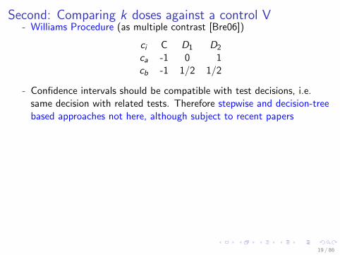
Second: Comparing k doses against a control V- Williams Procedure (as multiple contrast [Bre06])

ci C D1 D2

ca -1 0 1cb -1 1/2 1/2

- Confidence intervals should be compatible with test decisions, i.e.same decision with related tests. Therefore stepwise and decision-treebased approaches not here, although subject to recent papers

19 / 86

Second: Comparing k doses against a control VI- sCI should be estimated in the GLMM to consider several endpoint

types, allow covariates and secondary random factors

- One-sided (lower) simultaneous confidence limits:

[∑k

i=0 ci xi − Stq,df ,R,2−sided ,1−α

√∑ki c2

i /ni ]

- Example

−3 −2 −1 0 1

1000 − 0

500 − 0

250 − 0

125 − 0

62.5 − 0 (

(

(

(

(

)

)

)

)

)

95% family−wise confidence level

Linear Function

−2.0 −1.5 −1.0 −0.5

C 5

C 4

C 3

C 2

C 1 )

)

)

)

)

95% family−wise confidence level

Linear Function

20 / 86

Williams-type procedures for different endpoints I

- US-NTP recommends:

1 skewed-distributed endpoints (e.g. ASAT) nonparametric ⇒ yes, wecan

2 proportions ... arcsine transformation3 severity values ... Mann-Whitney test4 neoplasm lesions ... poly-k test (Bailer and Portier, 1988) ... a

survival-adjusted quantal-response procedure

- Here, Williams (Dunnett)-type procedures for

1 ratio-to-control2 relative effect size (e.g. for scores)3 proportions4 mortality5 poly-3 estimates6 dose-response relationships with downturn effect (muta-tox)

21 / 86

Williams-type procedures for different endpoints III Ratio-to-control: simultaneous confidence intervals for µi/µ0

ωi = ciµ/diµ

- ci and di are the i th row vector of C and D for numer./ denominator- Simply for Dunnett-type contrasts:

C =

0 0 0 10 0 1 00 1 0 0

D =

1 0 0 01 0 0 01 0 0 0

- The mratios R package [DSH07] can be used, here example exa1

95 % simultaneous CI (two−sided) for ratios (method: Plug−in)

1000/0

500/0

250/0

125/0

62.5/0

0.7 0.8 0.9 1.0 1.1 1.2

95 % simultaneous upper confidence limits for ratios (method: Plug−in)

Williams −type contrasts for ratios

C5

C4

C3

C2

C1

0.80 0.85 0.90 0.95 1.00

22 / 86

Williams-type procedures for different endpoints IIIII sCI when variance heterogeneity occurs

- Variance heterogeneity is quite common, i.e. εij ∼ N(0, σ2i ).

- Standard MCP do not control FWER, particularly for unbalanced ni

- Modified test statistic T 2∗(ωi ) = L(ωi )2/S2∗

L(ωi ), where

S2∗L(ωi ) =

ω2i

n0S2

0 +

q∑h=q+1−i

nh

n2i

S2h .

- T ∗(ωi ) has an approximate t-distribution with approximateSatterthwaite-type νUnder variance heterogeneity: both ν and R(ω) depend on theunknown ratios ωi and the unknown variances σ2

i

- Plug-in modification: sci.ratioVH function in the R package mratios[HH08]. Exa1 already used above

23 / 86

Williams-type procedures for different endpoints IV

III Non-parametric: simultaneous confidence intervals for relative effects

- The rank means can be used to estimate p0s

p0s =1

n0

(R

(0s)s· −

ns + 1

2

)- Asymptotically

√N(p1 − p1, . . . , pq − pq)′ follows a central

multivariate normal distribution with expectation 0 and covariancematrix VN [KH12a]

- Related approximate (1− α)100% one-sided lower simultaneousconfidence limits are:[

p` − tq,ν,R,1−α√

S`;], ` = 1, . . . , q, (1)

24 / 86

Williams-type procedures for different endpoints V- E.g. relative Shirley-type effects for order restriction [SHI77]

p1 = p0k

p2 =nk−1

nk−1 + nkp0(k−1) +

nk

nk−1 + nkp0k

...

pq =n1

n1 + . . .+ nkp01 + . . .+

nk

n1 + . . .+ nkp0k

- Example: next

25 / 86

Williams-type procedures for different endpoints VIIV Shirley-type test for graded histopathological findings using R package

nparcompOrdered categorical findings of non-neoplastic lesions in theP-Cresidine carcinogenicity study: hyperplasia in parotid glandlibrary(nparcomp)

nparcomp(Score~Group, data=parotid, asy.method = "probit",type="Williams", plot.simci = TRUE, info = TRUE)

exa2

Score

Gro

up

0 1 2 3

cont

rol

low

med

ium

|

|

|

|

0.0 0.1 0.2 0.3 0.4 0.5 0.6 0.7 0.8 0.9 1.0

p( c

ontr

ol ,

low

)p(

con

trol

, m

ediu

m ) 95 % Simultaneous Confidence Intervals

Type of Contrast: DunnettMethod: Probit − Transformation

|

|

|

|

0.0 0.1 0.2 0.3 0.4 0.5 0.6 0.7 0.8 0.9 1.0

C 1

C 2

95 % Simultaneous Confidence IntervalsType of Contrast: Williams

Method: Probit − Transformation

26 / 86

Williams-type procedures for different endpoints VIIV Tumor, incidence, mortality rates: 3 approaches Williams-type sCI for

proportions:

- Example: incidences of tubular epithelia hyaline droplet degenerationin male rats

Control Dose50 Dose75 Dose150with degeneration 2 6 4 13

n 32 27 32 21

1 Wald-type [HBW08]2 Add1- adjusted [SBH09]3 Profile likelihood [Ger10]

- For sample sizes of ni = 50...10 there is no hope for valid(1− α)100% Wald intervals. Therefore we need CIs with coverageprobability approximately 95% also for smaller samples

- And, for almost all proportions a one-sided alternative for an increaseis appropriate

27 / 86

Williams-type procedures for different endpoints VIII

- As effect size the difference of proportions is common (alternativelyrelative risk, OR)

- One-sided, lower (1− α)100% Wald-type confidence limits for thedifference of the proportions of treatment against those from acontrol are I∑

i=1

cipi − zq,R,1−α

√√√√ I∑i=1

c2i V (pi ) ;

(2)

with V (pi ) = pi (1− pi ) /ni and zq,R,1−α denoting the (1− α)quantile of the q-variate normal distribution

28 / 86

Williams-type procedures for different endpoints IX

- R depends not only on the known contrast coefficients cim andsample sizes ni but also on the unknown πi and V (pi ) where theplug-in of the ML-estimators πi and V (πi ) works well.

- [AC98] showed that adding a total of four pseudo-observations to theobserved successes and failures yields approximate confidence intervalsfor one binomial proportion with good small sample performance

- One-sided limits were investigated by [Cai05] in the case of a singlebinomial proportion I∑

i=1

ci pi − zq,R,1−α

√√√√ I∑i=1

c2i V (pi )

(3)

29 / 86

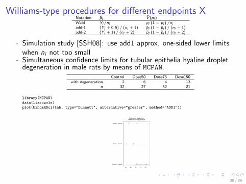
Williams-type procedures for different endpoints XNotation pi V (pi )Wald Yi/ni pi (1 − pi ) /niadd-1 (Yi + 0.5) / (ni + 1) pi (1 − pi ) / (ni + 1)add-2 (Yi + 1) / (ni + 2) pi (1 − pi ) / (ni + 2)

- Simulation study [SSH08]: use add1 approx. one-sided lower limitswhen ni not too small

- Simultaneous confidence limits for tubular epithelia hyaline dropletdegeneration in male rats by means of MCPAN.

Control Dose50 Dose75 Dose150with degeneration 2 6 4 13

n 32 27 32 21

library(MCPAN)

data(liarozole)

plot(binomRDci(tab, type="Dunnett", alternative="greater", method="ADD1"))

Proportion of patients with marked improvement

Dose150 − Placebo

Dose75 − Placebo

Dose50 − Placebo

−0.1 0.0 0.1 0.2 0.3

30 / 86

Williams-type procedures for different endpoints XI

VI Williams-type sCI for time-to-event data

- Williams-type proc. comparing survival functions: i) Cox proport.hazards model or ii) the frailty Cox model to allow a joint analysisover sex and strains [HH12]

-

- Example: Mortality data from the NTP no. TR-120 carcinogenicity ofpiperonyl butoxide Many observations were censored, mostly due toterminal sacrifice at day 784 (dose groups) and 826 (control); onlythree censored observations before: accidently killed or missing

C D1 D2

Events 5 12 16Early Censored 0 3 0Scheduled Sacrifice 15 35 34

31 / 86

Williams-type procedures for different endpoints XII

Days

Cum

ulat

ive

Sur

viva

l Rat

e

0 100 200 300 400 500 600 700 800

00.

20.

40.

60.

81

HighLowControl

- Effect size: Hazard rate. Using Williams-type sCI

Comparison Estimated HR sim. 97.5%-Interval

C vs. D2 3.83 [0.82,∞)C vs. (D1, D2) 3.18 [0.71,∞)

32 / 86

Williams-type procedures for different endpoints XIII

VII Williams-type procedure for poly-3 estimates

- In long-term carcinogenicity studies the compound may not only affectthe tumor rate but also the mortality in the treatment groups. Twoapproaches with/without cause-of-death information - here poly-ktrend test [BP88] only

- To account for censoring due to treatment-specific mortality,[BP88]

proposed the poly-3 adjustment by individual weights wij = (tij/tmax)k .- These weights result in an adjusted group sample size n∗

i =∑ni

j=1 wij

and therefore in adjusted proportions p∗i = yi/n∗

i .- [SSH08] demonstrated there plug-in instead of the crude proportions

into Dunnett/Williams procedure- Evaluation of the example: lower 95% Add-1 confidence limits to

detected an increasing trend in mortality-adjusted tumor rates

33 / 86

Williams-type procedures for different endpoints XIVdose 0 mg/kg 37 mg/kg 75 mg/kg 150 mg/kg

Crude Rate 1/50 9/50 8/50 5/50Crude Percent 2% 18% 16% 10%

Poly-3 adjusted-Rate 1/41.4 9/40.3 8/38.7 5/32.7Poly-3 adjusted-Percent 0.02% 0.22% 0.21% 0.15%

Table: Chronic toxicity study on methyleugenol

- Raw datagroup tumour death

1 0 0 3442 0 0 5213 0 0 5294 0 0 5535 0 0 5646 0 0 5887 0 0 6038 0 0 610.. ... ... ...

174 3 0 638175 3 0 642176 3 0 642177 3 0 642178 3 0 646179 3 0 648180 3 0 650181 3 0 654182 3 0 658183 3 0 659184 3 0 660185 3 0 660186 3 1 660187 3 1 660188 3 0 661189 3 0 669190 3 0 670191 3 0 680192 3 0 680193 3 1 683194 3 0 684195 3 0 688196 3 0 688197 3 0 699198 3 0 700199 3 0 704200 3 0 712

34 / 86

Williams-type procedures for different endpoints XVComparison estimate lower limit adjusted p-value

high vs. control 0.1288 −0.009 0.066high, medium vs. control 0.1555 0.048 0.005

high, medium, low vs. control 0.1701 0.075 0.0005

library(MCPAN)

data(methyl)

xtable(methyl)

poly3test(time=methyl$death, status=methyl$tumour,

f=methyl$group, type = "Williams", method = "ADD1", alternative="greater" )

C 3

C 2

C 1

0.00 0.05 0.10 0.15

35 / 86

Williams-type procedures for different endpoints XVIVIII US-NTP recommends the use of Dunnett and Williams procedure.

Which one really? Take both! (Jaki Hothorn 2013- Dun

cqi NC D1 D2 D3

ca -1 0 0 1cb -1 0 1 0cc -1 1 0 0

- Wilcqi NC D1 D2 D3

ca -1 0 0 1cb -1 0 1/2 1/2cc -1 1/3 1/3 1/3

- Dun and Wilcqi NC D1 D2 D3

ca -1 0 0 1cb -1 0 1/2 1/2cc -1 1/3 1/3 1/3cd -1 0 0 1ce -1 0 1 0cf -1 1 0 0

- UmbrellaWilcqi NC D1 D2 D3

ca -1 0 0 1cb -1 0 1/2 1/2cc -1 1/3 1/3 1/3cd -1 0 1 0ce -1 1/2 1/2 0cf -1 1 0 0

36 / 86

Williams-type procedures for different endpoints XVII- Example: Blood urea nitrogen content after 13 weeks repeated

administration of sodium dichromate dihydrate on male rats(NTP2012)

Comparison Dun Wil DuWi UWil1000 − 0 0.80 0.60 0.80 0.80500 − 0 6.8e-07 - 8.1e-07 8.4e-07250 − 0 0.110 - 0.11 0.12125 − 0 0.017 - 0.018 0.02062.5 − 0 0.045 - 0.047 0.051(1000 + 500)/2 − 0 - 0.0013 0.0030 0.0033(1000 + 500 + 250/3 − 0 - 0.0029 0.0057 0.0063(1000 + 500 + 250 + 125)/4 − 0 - 0.0021 0.0037 0.0042(1000 + 500 + 250 + 125 + 62.5)/5 − 0 - 0.0022 0.0039 0.0043(500 + 250)/2 − 0 - - - < 0.001(500 + 250 + 125)/3 − 0 - - - < 0.001(500 + 250 + 125 + 62.5)/4 − 0 - - - < 0.001(250 + 125)/2 − 0 - - - 0.023(250 + 125 + 62.5)/3 − 0 - - - 0.015(125 + 62.5)/2 − 0 - - - 0.015

37 / 86

Williams-type procedures for different endpoints XVIII

- Discussion:

95 % simultaneous CI (two−sided) for ratios (method: Plug−in)

C15

C14

C13

C12

C11

C10

C9

C8

C7

C6

C5

C4

C3

C2

C1

1.0 1.2 1.4

95 % simultaneous lower confidence limits for ratios (method: Plug−in)

C15

C14

C13

C12

C11

C10

C9

C8

C7

C6

C5

C4

C3

C2

C1

0.9 1.0 1.1 1.2 1.3 1.4

38 / 86

Williams-type procedures for different endpoints XIX

- Summary: i) For all endpoint types occurring in tox, Dunnett/Williams-type tests are available- together with related R libraries. Aunique proof of hazard approach for controlling FWER is available-use Williams tests recently [HCR+12, RSHK12] or Dunnett-type[SBHT12]ii) small sample size problems may be rather problematic

39 / 86

Unit II Evaluation of mutagenicity assays I

- What is specific in the analysis of mutagenicity assays?1 Most endpoints are counts, such as number of revertants. Therefore

appropriate procedures for the analysis of counts per experimentalunit(i.e. per animal or plate, xxx) are needed. Three approaches aredescribed: i) overdispersed Poisson in the GLM, ii) nonparametricapproach allowing ties and iii) data-transformation for the approximateuse of parametric approaches.

2 Alternatively, number at risk should be considered and thereforeprocedures for over-dispersed proportions are discussed. BEISPIEL

3 Moreover, continuous endpoints, such as lymph node weight areconsidered, where a log-transformation of the endpoint is quitecommon. The conditions and limitation for test assuming log-normaldistribution are discussed based on new functions in the library MCPAN

40 / 86

Unit II Evaluation of mutagenicity assays II

4 The concentrations used particularly in in-vitro assays are somewhatarbitrarily to human exposure. Furthermore, to avoid false negativeresults a tendency to over-dosing exists, and a so-called muta-toxproblem may occur, i.e. downturn effects at high(er) concentrations.Trend tests assuming strict order restriction may be seriously biasedand therefore a downturn-protected trend test and an one-sidedcomparison versus control without order restriction are proposed.Example Ames assay

5 Very small sample sizes are used in both in-vitro and in-vivo assays,such as triplicate plates in the Ames assay or 5 mice in themicronucleus assay. This rather critical limitation is discussed for theproposed statistical approaches.

6 In some assays the biological relevance is characterized by a certaink-fold change threshold. Therefore, procedure for ratio-to-control areproposed. Example LLNA assay

7 The role of the positive control to proof the current assay sensitivityExample micronucleus Hasler

8 Near-to-zero controls counts example HET-MN assays

41 / 86

Unit II Evaluation of mutagenicity assays III9 Direct use of historical data

10 Assuming a mixing distribution of many non-responders and someresponders Comet assay

42 / 86

Unit II Evaluation of mutagenicity assays IV

- Evaluation of the Ames Assay as an example for dose-response shapeswith possible downturn effectsThe tendency of over-dosing in in-vitro assays may cause a downturneffect at high(er) concentrations. Example Ames assay with TA98[MKZ81]:

Dose

y

2030

4050

60

0 10 33 100

333

1000

3 3 3 3 3 3

A clear downturn effect at doses higher than 100µg . For such a datasituation the use of:

43 / 86

Unit II Evaluation of mutagenicity assays V1 a global trend test with strict monotone alternative is clearly biased

(although the Williams-type approach is to some extend robust due totheir pooling-contrasts property)

2 n one-sided Dunnett-type approach is a possible alternative, althoughno trend claim for the lower doses is possible

3 a trend test up to the observerable top dose does not control a FWERand iv) therefore a multiple contrast test for all monotone alternativesup to all top doses was proposed [BH03] (see before in Unit I)

44 / 86

Unit II Evaluation of mutagenicity assays VI- Evaluation of the Ames Assay as an example for the analysis of a

design with rather small sample sizes: just triplicatesA challenge is the analysis of assays with rather small sample sizes,such as triplicate plates in the acid red 114 ames assay [HH03] Boththe non-parametric and the GLM-based approach are asymptotic onlyand violates the FWER at such small sample sizes. Considering thetradeoff between control of FWER and robustness, the parametricapproach may be the better alternative for such small sample countdata with a sufficient range of values.> revertant<-c(23,22,14,27,23,21,28,37,35,41,37,42)

> dose <- c(rep("control",3),rep("100mu",3),rep("333mu",3),rep("1000mu",3))

> amesHH <- data.frame(dose,revertant)

> library(multcomp)

> library(nparcomp)

> fitHHG <- lm(revertant~dose, data=amesHH)

> tstatG<-round(summary(glht(fitHHG, linfct = mcp(dose ="Williams")))$test$tstat[1],digits=2)

> tstatN<-round(nparcomp(revertant~dose, data=amesHH, type = "Williams", plot.simci = FALSE,

+ asy.method="mult.t", rounds=5, info=FALSE)$Analysis.of.relative.effects$t.value,digits=2)

> fitHHP <- glm(revertant~dose, data=amesHH, family=quasipoisson(link="log"))

> tstatP <- round(summary(glht(fitHHP, linfct = mcp(dose ="Williams")))$test$tstat[1],digits=2)

- Still a un-solved problem in biostatistics (-omics data). Discussion

45 / 86

Unit II Evaluation of mutagenicity assays VII- Evaluation of the LLNA as an example for k-fold rule

1 For selected muta-assays a relevance criteria was defined: i) the 2-foldrule for Ames assay [CP96], ii) a k = 1.55-fold increase for cellularity inBALB/c mice based on an interlaboratory study [EHH+05] in LLNA

2 I.e., relative change is used as effect size; here the ratio-to-controlversion of the Williams procedure is used assuming that cellularity isnormal distributed with heterogeneous variances [HD10], see [HV10].

n=6 n=6 n=6 n=6

5

10

15

20

25

Control Dlow Dmed Dxtrgroup

cell_

BA

LB

95 % simultaneous lower confidence limits for ratios (method: Plug−in)

Dxtr/Control

Dmed/Control

Dlow/Control

1.0 1.5 2.0 2.5 3.0

3 Interpretation

46 / 86

Unit II Evaluation of mutagenicity assays VIII4 What is common approach in tox/-omics? Log-transformation of the

endpoint, t-test and backtransformation. Is this appropriate? Answer

47 / 86

Unit II Evaluation of mutagenicity assays IX

- Evaluation of lymph node weight in the LLNA as an example oflog-normal distributed endpoints

1 The use of log-transformation is quite common in practice, to achieve amore symmetric distributed variable, a smaller impact of extremevalues, and reduction of variance heterogeneity. However, the effectsize switches from difference of arithmetic means to ratio of medians[Sch13]. Moreover, is the skewed distribution not approximatelylog-normal, transformation influences the other moments in a quitedifficult way.

Estimate lwr uprDlow - Control 1.37 1.05 Inf

Dmed - Control 1.61 1.24 InfDxtr - Control 3.03 2.33 Inf

2 If treatment effects develop in the skewness primarily (not just meanshifts as in RCT- a serious difference tox-to-clinics), i.e. more extremesingle value(s), the median is insensitive

48 / 86

Unit II Evaluation of mutagenicity assays X

3 Alternatively the ratios of expected values of log-normal distributionswere considered as effect sizes, i.e. future average fold change overmany replications (for log-normals) [Sch13]

4 If however, the variable is approximately log-normal distributed, e.g.which can be identified by comparing the two QQ-plots, simultaneousconfidence intervals for ratio-to-control means can be used based ongeneralized pivotal quantities. In the R package MCPAN a relatedfunction lnrci is available.

5 library(car)

library(MCPAN)

qqPlot(lm(cell_BALB~group, data=llna)) # raw data

qqPlot(lm(lcell~group, data=llna)) # log-transformed

gpqL<-lnrci(x=llna$lcell, f=llna$group, type="Dunnett", method="GPQ", B=40000, alternative="greater")

xtable(cbind(gpqL$estimate,gpqL$conf.int))

49 / 86

Unit II Evaluation of mutagenicity assays XI

−2 −1 0 1 2

−1

01

23

t Quantiles

Stu

dent

ized

Res

idua

ls(lm

(cel

l_B

ALB

~ g

roup

, dat

a =

llna

))

−2 −1 0 1 2

−2

−1

01

2

t Quantiles

Stu

dent

ized

Res

idua

ls(lm

(lcel

l ~ g

roup

, dat

a =

llna

))

V1 lower upper

Dlow / Control 1.17 0.97 InfDmed / Control 1.26 1.06 Inf

Dxtr / Control 1.61 1.35 Inf

50 / 86

Unit II Evaluation of mutagenicity assays XII

- Evaluation of HET-MN assay for an example using transformation ofcount data, particularly for near-to-zero counts in the controlMany statistical approaches have serious problems with this type ofdata, but two approaches may be appropriate: 1) FittingANOVA-type (MCP-type) approaches is not converting since the zerovariance in the control. An alternative is fitting a log-linear model forthe quantitative covariate log(conc) using the quasipoisson linkfunction in the glm, reporting the p-value of the slope for log(conc)

library(multcomp)

f1<-glm(y ~ DOSE, data=HMN, family=quasipoisson(link="log"))

summary(glht(f1, linfct = mcp(DOSE = "Dunnett")))

2) Alternatively the transformation of the counts according to[NOY03] can be used, and Williams-type test for difference-to-control.

51 / 86

Unit II Evaluation of mutagenicity assays XIII

n=6 n=6 n=6 n=6 n=60

10

20

0 0.375 0.75 1.5 3Dose

MN

95 % simultaneous lower confidence limits for ratios (method: Plug−in)

Williams −type contrasts for ratios

C4

C3

C2

C1

1.0 1.5 2.0

52 / 86

Unit II Evaluation of mutagenicity assays XIV

- Evaluation of the HET-MN assay for an example of using historicalcontrol data

1 HET-MN assay, i.e. the MN-induction in incubated hen eggs, wasintroduced [WNRB+08].

2 Specific is this assay because of the near-to-zero MN counts in thenegative control (see above)

3 To avoid false positive decisions, [WNRB+08] proposed the comparisonto the historical control counts when the concurrent counts are lessthan a σ interval of the historical mean. However, the p-value of thistest depends on the number of assays included in the historical database.

4 The negative controls:

53 / 86

Unit II Evaluation of mutagenicity assays XV

Interlaboratory Study− NC per run

exp

y

01

23

4

NC

6

A:06

NC

6

A:07

NC

6

B:07

NC

6

B:08

NC

6

B:09

NC

6

B:10

NC

6

B:11−1

6

B:11−2

3

C:01

4

C:02

6

C:03

5

C:04

6

C:05

01

23

4

6

C:06−AK

01

23

4

6

C:06−KM

6

C:06−SK

6

C:07−KM

6

C:07−SK

6

C:08−KM

6

C:08−SK

6

C:09−AK

6

C:09−KM

6

C:09−SK

6

C:10−AK

6

C:10−KM

01

23

4

6

C:11−SK

54 / 86

Unit II Evaluation of mutagenicity assays XVI

5 Considering binomial proportions in the historical control groups, whichcan be used to estimate the parameters of a beta prior distribution.This beta prior can be used for a multiple contrast test withaccordingly modified proportions [KHS12].

6 Alternatively, a parametric Williams-type procedure can be formulatedfor the comparison with a known standard)(instead of the concurrentcontrol when the control data are outside the historical normal range),namely the estimated mean of the historical controls ϑ [LR13]:

tvs.StandardContrast = (k∑

i=1

ci xi − ϑ)/Si=1,...,k

√√√√ k∑i=1

c2i /ni

55 / 86

Unit II Evaluation of mutagenicity assays XVII7 > library(qcc)

> HistNC$tN<-sqrt(HistNC$y)+ sqrt(HistNC$y+1)

> grp <- qcc.groups(HistNC$tN, HistNC$Run)

> qq<-qcc(grp, type="xbar", plot=FALSE)

> Tnormalval<-limits.xbar.one(center=qq$center, std.dev=qq$std.dev,conf=2)

> nm <- lm(tN ~ 1, data=HistNC)

> nKfix <- coefficients(nm)

> myHETMN$Dose<-as.factor(myHETMN$dose)

> myHETMNco <- droplevels(subset(myHETMN, Dose == 0))

> meanCO<-mean(myHETMNco$tN)

> myHETMNno <- droplevels(subset(myHETMN, Dose != 0))

> nam <- lm(tN ~ Dose-1, data=myHETMNno)

> library(multcomp)

> design<-summary(myHETMN$Dose)

> cmatrix<-contrMat(design, type="Williams")[,-1]

> ngw <- glht(nam, linfct=cmatrix, rhs=nKfix)

> summary(ngw)

> modConcur<-lm(tN~Dose, data=myHETMN) # versus concurrent control

> summary(glht(modConcur, linfct = mcp(Dose = "Williams")))

56 / 86

Unit II Evaluation of mutagenicity assays XVIII

- Evaluation of the in vivo micronucleus assay as an example ofoverdispersed proportion

1 In the in vivo micronucleus assay according to guideline [47406] is theprimary endpoint is the number micronucleited erythocytes (MN) per acertain number of scored polychromatic erythrocytes (PCE), peranimal.

2 In some assays the number of scored cells is constant, such as the 2000scored cells in the assay with 1-phenylethanol [Eng06]

3 In other assays rather different number of scored cells occur such in themicroneucleus assay with 5-(4-Nitrophenyl)-2,4-pentadien-1-al on theperipherical blood of B6C3F1 mice

57 / 86

Unit II Evaluation of mutagenicity assays XIXDose Animal PCE MN MNP risk

1 Control 1.00 15154.00 22.00 1.50 15132.002 Control 10.00 11063.00 14.00 1.30 11049.003 Control 2.00 10384.00 19.00 1.80 10365.004 Control 3.00 12094.00 9.00 0.70 12085.005 Control 4.00 11577.00 16.00 1.40 11561.006 Control 5.00 12050.00 13.00 1.10 12037.007 Control 6.00 10316.00 7.00 0.70 10309.008 Control 7.00 9896.00 27.00 2.70 9869.009 Control 8.00 12032.00 17.00 1.40 12015.00

10 Control 9.00 12981.00 12.00 0.90 12969.0011 D0.03 11.00 10138.00 21.00 2.10 10117.0012 D0.03 12.00 12864.00 16.00 1.20 12848.0013 D0.03 13.00 12464.00 14.00 1.10 12450.0014 D0.03 14.00 10220.00 9.00 0.90 10211.0015 D0.03 15.00 13411.00 18.00 1.30 13393.0016 D0.03 16.00 12148.00 53.00 4.40 12095.0017 D0.03 17.00 10987.00 21.00 1.90 10966.0018 D0.03 18.00 10290.00 20.00 1.90 10270.0019 D0.03 19.00 11627.00 18.00 1.50 11609.0020 D0.03 20.00 11872.00 23.00 1.90 11849.0021 D0.1 21.00 11381.00 6.00 0.50 11375.0022 D0.1 22.00 9860.00 12.00 1.20 9848.0023 D0.1 23.00 9776.00 16.00 1.60 9760.0024 D0.1 24.00 9944.00 16.00 1.60 9928.0025 D0.1 25.00 11141.00 15.00 1.30 11126.0026 D0.1 26.00 10941.00 12.00 1.10 10929.0027 D0.1 27.00 10705.00 20.00 1.90 10685.0028 D0.1 28.00 11790.00 14.00 1.20 11776.0029 D0.1 29.00 9760.00 10.00 1.00 9750.0030 D0.1 30.00 12214.00 23.00 1.90 12191.0031 D0.3 31.00 11912.00 20.00 1.70 11892.0032 D0.3 32.00 10672.00 27.00 2.50 10645.0033 D0.3 33.00 10498.00 15.00 1.40 10483.0034 D0.3 34.00 11479.00 16.00 1.40 11463.0035 D0.3 35.00 13579.00 29.00 2.10 13550.0036 D0.3 36.00 14141.00 21.00 1.50 14120.0037 D0.3 37.00 12714.00 19.00 1.50 12695.0038 D0.3 38.00 10723.00 13.00 1.20 10710.0039 D0.3 39.00 10552.00 14.00 1.30 10538.0040 D0.3 40.00 11725.00 26.00 2.20 11699.0041 D1 41.00 12194.00 32.00 2.60 12162.0042 D1 42.00 13567.00 24.00 1.80 13543.0043 D1 43.00 12786.00 27.00 2.10 12759.0044 D1 44.00 10228.00 21.00 2.10 10207.0045 D1 45.00 9548.00 14.00 1.50 9534.0046 D1 46.00 13064.00 24.00 1.80 13040.0047 D1 47.00 14362.00 36.00 2.50 14326.0048 D1 48.00 11805.00 31.00 2.60 11774.0049 D1 49.00 12548.00 24.00 1.90 12524.0050 D1 50.00 10979.00 37.00 3.40 10942.0051 D3 51.00 12654.00 77.00 6.10 12577.0052 D3 52.00 10599.00 34.00 3.20 10565.0053 D3 53.00 9898.00 47.00 4.70 9851.0054 D3 54.00 12084.00 49.00 4.10 12035.0055 D3 55.00 11389.00 59.00 5.20 11330.0056 D3 56.00 9760.00 46.00 4.70 9714.0057 D3 57.00 9970.00 53.00 5.30 9917.0058 D3 58.00 9766.00 63.00 6.50 9703.0059 D3 59.00 12340.00 63.00 5.10 12277.0060 D3 60.00 9970.00 32.00 3.20 9938.00

58 / 86

Unit II Evaluation of mutagenicity assays XX

4 Therefore the analysis of overdispersed proportions MN/PCE isappropriate.

5 In the in vivo micronucleus assay, clearly the individual animal is theexperimental unit, it is randomized, it is treated. Therefore, thevariability between the animals should be taken into account.

6 Hence, pooling the number of MN over the animals of a group, asproposed [KCK00], results in too liberal decisions and can not berecommended.

7 This between animals variability can be considered for example by aquasi-binomial model, where a dispersion parameter is estimated fromthe data, characterizing this between animals variability [PS07].

8 A second statistical aspect is the use of confidence intervals for anappropriate effects size, such as odds ratio (OR) or risk ratio (RR).

59 / 86

Unit II Evaluation of mutagenicity assays XXI

9 Confidence intervals can be estimated for the odds ratio (OR) usingthe common logit link function in the quasi-binomial model. Becausethe ORs are not easy to understand and differ not seriously from

relative risks RRiC = MNi/PCEi

MNC/PCECfor small proportions, and 2 MN per

2000 PCE is a small proportion, alternatively the quasi-binomial modelwith the log link function is used.

RRPH lowerquaPD0.03 - Control 1.38 1.04

D0.1 - Control 1.01 0.74D0.3 - Control 1.28 0.96

D1 - Control 1.68 1.28D3 - Control 3.63 2.85

Table: Pairwise relative risks on overdispersed proportions withoutFWER control - NPPD

60 / 86

Unit II Evaluation of mutagenicity assays XXIIRRPHo lowerquaPo

D0.03 - Control 1.38 1.16D0.1 - Control 1.01 0.83D0.3 - Control 1.28 1.07

D1 - Control 1.68 1.42D3 - Control 3.63 3.13

Table: Pairwise relative risks on pooled proportions without FWERcontrol - NPPD

10 The estimated dispersion parameter is 2.67, indicating anoverdispersion, i.e. a serious between animals variability and thereforelower confidence limits ignoring this variability (lowerRRbin) are tooliberal, i.e. with a tendency of false positive decisions.

61 / 86

Unit II Evaluation of mutagenicity assays XXIII

- Evaluation of the in-vitro micronucleus assay as an example forcomparing distributions of nucleated cellsAccording to the OECD guideline, the distribution of mono-, bi-, tri-and tetra-nucleated cells should be considered. After the exposure toX-ray radiation (in Gy) [HCJJ00] presented in its Tab. 2 the numberof cytokinesis-blocked micronucleus (CBMN) with number of cellscarrying one, two, and three MN; see Table 4. Although this type ofdata can be rarely find in the literature and the evaluation and itsinterpretation is not simple, a related approach will be provided here.

62 / 86

Unit II Evaluation of mutagenicity assays XXIV

group donor NC one two three total1 control a 1000 8 0 0 82 d0.02 a 1000 10 0 0 103 d0.05 a 1000 16 0 0 164 d0.10 a 1000 14 0 0 145 d0.25 a 1000 23 1 0 246 d0.50 a 1000 24 2 0 267 d1.00 a 1000 36 5 0 418 d2.00 a 1000 53 7 2 629 control b 1000 7 0 0 7

10 d0.02 b 1000 8 0 0 811 d0.05 b 1000 7 0 0 712 d0.10 b 1000 9 0 0 913 d0.25 b 1000 11 0 0 1114 d0.50 b 1000 16 1 0 1715 d1.00 b 1000 24 2 0 2616 d2.00 b 1000 56 4 1 61

Table: Mono-, bi- and tri-nucleated cell counts

By pooling over cultures, the data can be simplified to a 4× k table.

63 / 86

Unit II Evaluation of mutagenicity assays XXVdose NC one two three total

1 control 2000 15 0 0 152 d0.02 2000 18 0 0 183 d0.05 2000 23 0 0 234 d0.10 2000 23 0 0 235 d0.25 2000 34 1 0 356 d0.50 2000 40 3 0 437 d1.00 2000 60 7 0 678 d2.00 2000 109 11 3 123

Table: Mono-, bi- and tri-nucleated cell counts pooled over cultures

If additional information about the number of counts is available,these can be treated as independent endpoints with the methodsdescribed above. In addition these counts can be assumed to follow amultinomial distribution, as the complete number of NCs is known.Multinomial models can be fitted in R with the add-on packageVGAM. In an exemplary multinomial baseline category model thecounts for each group (one, two, three) are related to the a fourthgroup of no micronuclei counted. The sum of all theses counts givethe complete number of NCs observed. This kind of multinomialmodel can be fit in R by

> library(VGAM)

> fitbase <- vglm(cbind(one,two,three,NC-total) ~ dose, multinomial, hep)

64 / 86

Unit III The alternative: significant toxicity approach I

- The significant toxicity approach [DDZ11] uses first time in regulatorytoxicology a proof of safety approach (for selected aquatic assays)with 6 important features:

1 controlling the more important false negative decision rate directly2 formulating one-sided hypotheses for claiming non-inferiority, i.e.

non-relevant (tolerable) toxicity3 proposing a ratio-to-control test instead of the wide-spread used

difference-to-control tests4 defining assay-specific non-inferiority thresholds, for chronic assaysδ = 0.75 and for acute assays δ = 0.80

5 proposing assay-specific α rates to achieve a balanced false negative-to-falsepositive decision ratio

6 characterisation of the assay-specific false positive rates by means of

simulations

- Three different types of endpoints can be distinguished intoxicological assays:

65 / 86

Unit III The alternative: significant toxicity approach II

1 vital signs functions, e.g. number of offsprings per alive female inCeriodaphnia dubia assay [MVB12]

2 outcomes of a specific pathological process, e.g. number of micronucleiin the MN assay [HG09]

3 outcomes of a general physiological process, e.g. serum bilirubincontent [AAAA12].

- Assays with the first endpoint, denoted here as bfinhibition assays, areparticularly suitable for ratio-to-control tests on non-inferiority, sincetheir continuous, count, or proportion endpoint decreases from largevalues in the control (sometimes 100%) to small values in theconcentration groups as a sign of toxicity, e.g. reduction the numberof offsprings

- Contrarily, in the second endpoint type, the data in the control are often zero or

near-to-zero; but ratio-to-control tests require an appropriate large mean value in the

control (relative to its standard deviation and sample size) [? ]. For the third endpoint

type increases or decreases may of toxicological interest, i.e. two-sided hypotheses are

appropriate.

66 / 86

Unit III The alternative: significant toxicity approach III- Although a controversy on the appropriateness of one-sided tests

exists (see, e.g. [? ]), one-sided tests for endpoints in inhibitionassays are clearly recommended, since the other direction istoxicologically irrelevant. Moreover, one-sided hypothesis areinherently needed for non-inferiority test.

- Non-inferiority tests are originally defined for a primary efficacyendpoint in randomized clinical trials, to accept new drugs whichreveals a tolerable less efficacy, based on an a-priori defined margin η,but with other advantages, such as lower price, or less side effects.

- In toxicology, the tests with a direct control of the more importantfalse negative control (be confident in negative results) were denotedas proof-of-safety [Bro85]. The major difference is to use one-sidedtests on non-inferiority instead of two-sided tests on equivalence[HBW08]).

- Notice, be confident in negative results is the aim in tox riskassessment ⇒ proof of safety is appropriate

67 / 86

Unit III The alternative: significant toxicity approach IV

- However, most studies in tox are not (planned) and analyzed by proofof safety

- A motivating example Aquatic assay on Ceriodaphnia dubia [BO94]treated with nitrofen. In the assay, 50 animals were randomized intobatches of 10 and each batch was put in a solution with a selectedconcentration of nitrofen. The number of total live offspringssummarized of the three broods to each animal was used as anendpoint. In the box-plot (blue ... x , SD, red ... individual counts):

68 / 86

Unit III The alternative: significant toxicity approach V

n=10 n=10 n=10 n=10 n=10 n=100

10

20

30

40

0 1.56 3.12 6.25 12.5 25conc

NoY

- Although the data are counts, according to the wide range of valuesbetween zero and 36 the assumption of normal distribution may beappropriate.

69 / 86

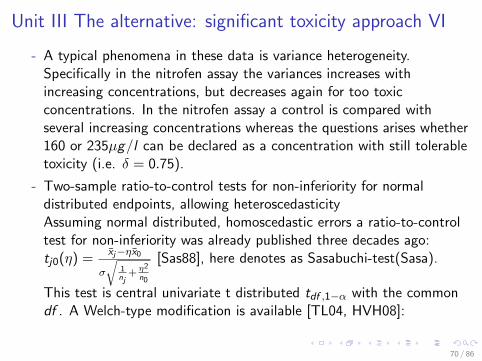
Unit III The alternative: significant toxicity approach VI

- A typical phenomena in these data is variance heterogeneity.Specifically in the nitrofen assay the variances increases withincreasing concentrations, but decreases again for too toxicconcentrations. In the nitrofen assay a control is compared withseveral increasing concentrations whereas the questions arises whether160 or 235µg/l can be declared as a concentration with still tolerabletoxicity (i.e. δ = 0.75).

- Two-sample ratio-to-control tests for non-inferiority for normaldistributed endpoints, allowing heteroscedasticityAssuming normal distributed, homoscedastic errors a ratio-to-controltest for non-inferiority was already published three decades ago:tj0(η) =

xj−ηx0

σ

√1nj

+ η2

n0

[Sas88], here denotes as Sasabuchi-test(Sasa).

This test is central univariate t distributed tdf ,1−α with the commondf . A Welch-type modification is available [TL04, HVH08]:

70 / 86

Unit III The alternative: significant toxicity approach VII

tWelch−typej0 (η) =

xj−ηx0√s2j /nj+

s20η2

n0

using the Welch df Welch−type , denotes

as Tamhane-Logan-Test (TamhLog).

- Analysis of the example: Unadjusted ratios-to-control with δ = 0.75

1 Using unadjusted two-sample Sasabuchi-tests (corrected againstvariance heterogeneity)-

2 with δ’s AND the other direction (inhibition means decreasing effect,but test direction is increase for non-inferiority)

3 Explain the appropriate limit using two-sided CIs

71 / 86

Unit III The alternative: significant toxicity approach VIII

95 % unadjusted CI (two−sided) for ratios

12.5/0

6.25/0

3.12/0

1.56/0

0.5 1.0 1.5 2.0

4 Still safe is when the upper limit is > δ = 0.75 ; otherwise unsafe5 Safe are 1.56, 3.12, 6.25 but NOT 12.56 The correct upper limit needs i) one-sided testing, ii) the following

code in library(mratios)sci.ratioVH(NoY~conc, data=daphn, type = "Dunnett", base = 1, alternative = "less",method="Unadj")

simtest.ratioVH(NoY~conc, data=daphn, type = "Dunnett", Margin.vec=c(0.75, 0.75, 0.75, 0.75), base = 1, alternative = "less") ## take p.value.raw!

72 / 86

Unit III The alternative: significant toxicity approach IX

95 % unadjusted upper confidence limits for ratios

12.5/0

6.25/0

3.12/0

1.56/0

0.5 1.0 1.5 2.0

7 Interprete8 Explain test (unad. p-values) vs. upper confidence limits

- Further aspects

73 / 86

Unit IV: Final discussion I

- Visualize the data, e.g. grouped by jittered box-plots

- Use pairwise Welch-tests or Dunnett&Williams-Satterthwaiteprocedure. Avoid: F-, Kruskal-Wallis-, Tukey-, Scheffe-, Duncan-,asymptotic Wilcoxon-test

- Use confidence intervals instead of p-values or ***

- Use parametric tests as long as ....

- CR: Use 5PL model to estimate EC50, take further random effectsinto account

- Use R

74 / 86

Excercise 1 I

- Using R (needed libraries: mratios, )

- How to import data?

1 directly xls file2 read a ASCII file (csv)3 load an internal *.rda file

- A jittered box-plot is suitable for data presentation

1 median to mean shows distribution behavior2 interquartile range and SD shows variance homogeneity/heterogeneity

(in relation to sample sizes)3 individual values and their distribition (e.g. skewness, ties) can be seen4 extreme values can be identified

-

75 / 86

Excercise 2: Welch-test I

- use ntp data

- provide jittered box-plots

- characterize data

- use library(pairwiseCI)

- use p-values and CIs

76 / 86

Excercise 3. Ames Assay I

- use

library(flexmix)

data("salmonellaTA98")

-

77 / 86

Excercise 4: MN Assay I

- use

library(mratios)

data("Mutagenicity")

-

78 / 86

References I[47406] 474, OECD: OECD Guideline for testing of chemicals: In vivo micronucleus test / OECD/OCDE 474. 2006. –

Forschungsbericht

[AAAA12] Adaramoye, O. A. ; Adesanoye, O. A. ; Adewumi, O. M. ; Akanni, O.: Studies on the toxicological effect ofnevirapine, an antiretroviral drug, on the liver, kidney and testis of male Wistar rats. In: Hum Exp Toxicol 31(2012), Nr. 7, S. 676–685. http://dx.doi.org/10.1177/0960327111424304. – DOI10.1177/0960327111424304. – ISSN 0960–3271

[AC98] Agresti, A. ; Coull, B. A.: Approximate is better than ”exact” for interval estimation of binomial proportions.In: American Statistician 52 (1998), Mai, Nr. 2, S. 119–126

[BH03] Bretz, F ; Hothorn, LA: Statistical analysis of monotone or non-monotone dose-response data from in vitrotoxicological assays. In: ATLA-Altern Lab Anim 31 (2003), JUN, Nr. Suppl. 1, S. 81–96. – ISSN 0261–1929

[BM00] Brunner, E. ; Munzel, U.: The nonparametric Behrens-Fisher problem: Asymptotic theory and a small-sampleapproximation. In: Biometrical Journal 42 (2000), Nr. 1, S. 17–25

[BO94] Bailer, A.J. ; Oris, J.T. ; al., N. L. (Hrsg.): Assessing toxicity of pollutants in aquatic systems. John Wiley,1994

[BP88] Bailer, A.J. ; Portier, C. J.: Effects Of Treatment-Induced Mortality And Tumor-Induced Mortality On TestsFor Carcinogenicity In Small Samples. In: Biometrics 44 (1988), Juni, Nr. 2, S. 417–431

[Bre06] Bretz, Frank: An Extension of the Williams Trend Test to General Unbalanced Linear Models. In: Comput.Stat. Data An. 50 (2006), Nr. 7, S. 1735–1748

[Bro85] Bross, I. D.: Why Proof Of Safety Is Much More Difficult Than Proof Of Hazard. In: Biometrics 41 (1985), Nr.3, S. 785–793

[Cai05] Cai, T. T.: One-sided confidence intervals in discrete distributions. In: Journal Of Statistical Planning AndInference 131 (2005), April, Nr. 1, S. 63–88

[CP96] Cariello, N. F. ; Piegorsch, W. W.: The Ames test: The two-fold rule revisited. In: MutationResearch-Genetic Toxicology 369 (1996), Juli, Nr. 1-2, S. 23–31

[DDZ11] Denton, Debra L. ; Diamond, Jerry ; Zheng, Lei: Test of significance in toxicity: A statistical application forassessing whether an effluent or site water is truly toxic. In: Environ Toxicol Chem 30 (2011), MAY, Nr. 5, S.1117–1126. http://dx.doi.org/10.1002/etc.493. – DOI 10.1002/etc.493. – ISSN 0730–7268

79 / 86

References II[DSH07] Dilba, G. ; Schaarschmidt, F. ; Hothorn, L.A.: Inferences for ratios of normal means. In: R News 7 (2007),

S. 20–23

[Dun55] Dunnett, C. W.: A Multiple Comparison Procedure For Comparing Several Treatments With A Control. In: JAm Stat Assoc 50 (1955), Nr. 272, S. 1096–1121

[EHH+05] Ehling, G. ; Hecht, M. ; Heusener, A. ; Huesler, J. ; Gamer, A. O. ; Loveren, H. van ; Maurer, T. ;Riecke, K. ; Ullmann, L. ; Ulrich, P. ; Vandebriel, R. ; Vohr, H. W.: An European inter-laboratoryvalidation of alternative endpoints of the murine local lymph node assay - 2nd round. In: Toxicology 212 (2005),August, Nr. 1, S. 69–79

[Eng06] Engelhardt, G.: In vivo micronucleus test in mice with 1-phenylethanol. In: Archives Of Toxicology 80 (2006),Dezember, Nr. 12, S. 868–872

[Fie54] Fieller, E. C.: Some Problems In Interval Estimation. In: Journal Of The Royal Statistical Society SeriesB-Statistical Methodology 16 (1954), Nr. 2, S. 175–185

[Ger10] Gerhard, D.: Simultaneous small sample inference based on profile likelihood / Leibniz University Hannover.2010. – Forschungsbericht

[Hay13] Hayter, A. J.: Inferences on the difference between future observations for comparing two treatments. In:JOURNAL OF APPLIED STATISTICS 40 (2013), APR 1, Nr. 4, S. 887–900.http://dx.doi.org/10.1080/02664763.2012.758245. – DOI 10.1080/02664763.2012.758245. – ISSN0266–4763

[HBW08] Hothorn, Torsten ; Bretz, Frank ; Westfall, Peter: Simultaneous Inference in General Parametric Models.In: Biometrical J 50 (2008), Nr. 3, S. 346–363

[HCJJ00] He, J. L. ; Chen, W. L. ; Jin, L. F. ; Jin, H. Y.: Comparative evaluation of the in vitro micronucleus test andthe comet assay for the detection of genotoxic effects of X-ray radiation. In: Mutation Research-GeneticToxicology And Environmental Mutagenesis 469 (2000), September, Nr. 2, S. 223–231

[HCR+12] Hobbs, Cheryl A. ; Chhabra, Rajendra S. ; Recio, Leslie ; Streicker, Michael ; Witt, Kristine L.:Genotoxicity of styrene-acrylonitrile trimer in brain, liver, and blood cells of weanling F344 rats. In:ENVIRONMENTAL AND MOLECULAR MUTAGENESIS 53 (2012), APR, Nr. 3, S. 227–238.http://dx.doi.org/10.1002/em.21680. – DOI 10.1002/em.21680. – ISSN 0893–6692

80 / 86

References III[HD10] Hothorn, L.A. ; Dilba, G.D.: A ratio-to-control Williams-type test for trend. In: Pharmaceutical Statistics 11

(2010), S. 1111

[HG09] Hothorn, L. A. ; Gerhard, D.: Statistical evaluation of the in vivo micronucleus assay. In: Arch Toxicol 83(2009), Nr. 6, S. 625–634

[HH03] Hauschke, D. ; Hothorn, L. A.: Two-stage testing of safety: A statistical view. In: Atla-Alternatives ToLaboratory Animals 31 (2003), Juni, S. 77–80

[HH08] Hasler, M. ; Hothorn, L.A.: Multiple contrast tests in the presence of heteroscedasticity. In: Biometrical J 51(2008), S. 1

[HH12] Herberich, Esther ; Hothorn, Ludwig A.: Statistical evaluation of mortality in long-term carcinogenicitybioassays using a Williams-type procedure. In: Regul Toxicol Pharm 64 (2012), S. 26–34

[HV10] Hothorn, L. A. ; Vohr, H. W.: Statistical evaluation of the Local Lymph Node Assay. In: RegulatoryToxicology and Pharmacology 56 (2010), April, Nr. 3, S. 352–356

[HVH08] Hasler, M. ; Vonk, R. ; Hothorn, L. A.: Assessing non-inferiority of a new treatment in a three-arm trial inthe presence of heteroscedasticity. In: Statistics In Medicine 27 (2008), Februar, Nr. 4, S. 490–503

[KCK00] Kim, B. S. ; Cho, M. H. ; Kim, H. J.: Statistical analysis of in vivo rodent micronucleus assay. In: MutationResearch-Genetic Toxicology And Environmental Mutagenesis 469 (2000), September, Nr. 2, S. 233–241

[KH12a] Konietschke, Frank ; Hothorn, Ludwig A.: Evaluation of Toxicological Studies Using a Non-ParametricShirley-type Trend Test for Comparing Several Dose Levels With a Control Group. In: Stat Biopharm Res 4(2012), S. 14–27

[KH12b] Konietschke, Frank ; Hothorn, Ludwig A.: Rank-based multiple test procedures and simultaneous confidenceintervals. In: Electron J Stat 6 (2012), S. 738–759. http://dx.doi.org/10.1214/12-EJS691. – DOI10.1214/12–EJS691. – ISSN 1935–7524

[KHS12] Kitsche, A. ; Hothorn, L. A. ; Schaarschmidt, F.: The use of historical controls in estimation simultaneousconfidence intervals for comparisons against a concurrent control. In: Computational Statistics and Data Analysis56 (2012), Nr. 12, S. 3865–3875

[LR13] L.A., Hothorn ; Reisinger, et a. K.: Statistical analysis of the hens egg test for micronucleus induction(HET-MN Assay). In: Mutation Res xx (2013), S. bb

81 / 86

References IV

[MKZ81] Margolin, B. H. ; Kaplan, N. ; Zeiger, E.: Statistical-Analysis of the Ames Salmonella-Microsome Test. In:Proceedings Of The National Academy Of Sciences Of The United States Of America-Biological Sciences 78(1981), Nr. 6, S. 3779–3783

[MVB12] Manar, Rachid ; Vasseur, Paule ; Bessi, Hlima: Chronic toxicity of chlordane to Daphnia magna andCeriodaphnia dubia: A comparative study. In: Environ Toxicol 27 (2012), Nr. 2, S. 90–97.http://dx.doi.org/10.1002/tox.20616. – DOI 10.1002/tox.20616. – ISSN 1520–4081

[NOY03] Nishiyama, H. ; Omori, T. ; Yoshimura, I.: A composite statistical procedure for evaluating genotoxicity usingcell transformation assay data. In: Environmetrics 14 (2003), Marz, Nr. 2, S. 183–192.http://dx.doi.org/10.1002/env.575. – DOI 10.1002/env.575

[PS07] Paul, S. ; Saha, K. K.: The generalized linear model and extensions: a review and some biological andenvironmental applications. In: Environmetrics 18 (2007), Juni, Nr. 4, S. 421–443

[RA08] Ryu, E. J. ; Agresti, A.: Modeling and inference for an ordinal effect size measure. In: Statistics In Medicine 27(2008), Mai, Nr. 10, S. 1703–1717

[RSHK12] Recio, Leslie ; Shepard, Kim G. ; Hernandez, Lya G. ; Kedderis, Gregory L.: Dose-Response Assessment ofNaphthalene-Induced Genotoxicity and Glutathione Detoxication in Human TK6 Lymphoblasts. In: ToxicologicalSciences 126 (2012), April, Nr. 2, S. 405–412. http://dx.doi.org/10.1093/toxsci/kfs012. – DOI10.1093/toxsci/kfs012

[Sas88] Sasabuchi, S: A multivariate one-sided test with composite hypotheses whne the covariance matrix is completelyunknown. In: Memoirs of the Faculty of Science, Series A 42 (1988), S. 37–46

[SBH09] Schaarschmidt, F. ; Biesheuvel, E. ; Hothorn, L. A.: Asymptotic Simultaneous Confidence Intervals forMany-to-One Comparisons of Binary Proportions in Randomized Clinical Trials. In: Journal of BiopharmaceuticalStatistics 19 (2009), Nr. 2, S. 292–310

[SBHT12] Schardein, James L. ; Birch, Robert ; Hesley, Robb ; Thorsrud, Bjorn A.: Multigeneration ReproductiveStudy of Hydroxyprogesterone Caproate (HPC) in the Rat: Laboratory Results and Clinical Significance. In:BIRTH DEFECTS RESEARCH PART B-DEVELOPMENTAL AND REPRODUCTIVE TOXICOLOGY 95 (2012),APR, Nr. 2, S. 160–174. http://dx.doi.org/10.1002/bdrb.21000. – DOI 10.1002/bdrb.21000. – ISSN1542–9733

82 / 86

References V

[Sch13] Schaarschmidt, Frank: Simultaneous confidence intervals for multiple comparisons among expected values oflog-normal variables. In: COMPUTATIONAL STATISTICS & DATA ANALYSIS 58 (2013), FEB, S. 265–275.http://dx.doi.org/10.1016/j.csda.2012.08.011. – DOI 10.1016/j.csda.2012.08.011. – ISSN 0167–9473

[SHI77] SHIRLEY, E: NONPARAMETRIC EQUIVALENT OF WILLIAMS TEST FOR CONTRASTING INCREASINGDOSE LEVELS OF A TREATMENT. In: BIOMETRICS 33 (1977), Nr. 2, S. 386–389. – ISSN 0006–341X

[SSH08] Schaarschmidt, F. ; Sill, M. ; Hothorn, L. A.: Poly-k-trend tests for survival adjusted analysis of tumor ratesformulated as approximate multiple contrast test. In: J Biopharm Stat 18 (2008), Nr. 5, S. 934–948

[TL04] Tamhane, M. C. ; Logan, B. R.: A superiority-equivalence approach to one-sided tests on multiple endpoints inclinical trials. In: Biometrika 91 (2004), September, Nr. 3, S. 715–727

[WNRB+08] Wolf, T. ; Niehaus-Rolf, C. ; Banduhn, N. ; Eschrich, D. ; Scheel, J. ; Luepke, N-P.: The hen’s egg testfor micronucleus induction (HET-MN): Novel analyses with a series of well-characterized substances support thefurther evaluation of the test system. In: Mutation Research-Genetic Toxicology and Environmental Mutagenesis650 (2008), Nr. 2, S. 150–164

[WSI+07] Woo, G. H. ; Shibutani, M. ; Ichiki, T. ; Hamamura, M. ; Lee, K. Y. ; Inoue, K. ; Hirose, M.: A repeated28-day oral dose toxicity study of nonylphenol in rats, based on the ’Enhanced OECD Test Guideline 407’ forscreening of endocrine-disrupting chemicals. In: Archives Of Toxicology 81 (2007), Februar, Nr. 2, S. 77–88

Supported in part by the EC FP7 program project ESNATS

83 / 86

Appendix : Raw data I- The NTP Isoniazid data : ntp.cvs

Anino Dose BUN TP ALB Globulin Glucose SGPT1 043 0.00 12.14 5.40 4.00 1.40 214.00 28.182 044 0.00 13.42 5.90 4.25 1.70 235.00 20.063 045 0.00 20.77 6.10 4.05 2.10 242.00 23.614 046 0.00 27.31 6.00 3.95 2.10 263.00 27.175 047 0.00 14.24 6.10 4.10 2.00 227.00 25.906 048 0.00 8.29 6.20 3.65 2.50 248.00 22.857 049 25.00 17.39 6.50 3.87 2.60 187.00 21.338 050 25.00 23.46 6.40 4.01 2.40 254.00 18.289 051 25.00 13.54 5.90 3.99 1.90 227.00 18.03

10 052 25.00 18.09 5.90 3.77 2.20 219.00 20.8211 053 25.00 25.09 6.60 3.64 3.00 252.00 16.7612 054 25.00 16.69 6.00 3.95 2.10 266.00 23.6113 055 50.00 19.96 5.80 3.92 1.90 210.00 18.0314 056 50.00 21.59 6.40 4.15 2.30 199.00 22.6015 057 50.00 21.47 5.90 3.85 2.00 205.00 27.1716 058 50.00 19.26 6.40 3.83 2.60 181.00 20.5717 059 50.00 14.94 6.10 3.92 2.20 243.00 24.8818 060 50.00 9.92 6.00 4.00 2.00 243.00 25.3919 061 100.00 10.15 6.00 3.97 2.10 231.00 19.5520 062 100.00 17.27 6.30 4.19 2.10 238.00 21.8421 063 100.00 21.59 5.60 3.75 1.90 239.00 24.8822 064 100.00 22.99 6.20 3.92 2.20 247.00 22.8523 065 100.00 22.76 5.40 3.67 1.70 231.00 17.7724 066 100.00 28.71 5.40 3.98 1.40 230.00 19.3025 067 150.00 26.14 7.20 3.90 3.30 230.00 15.7426 068 150.00 20.66 6.00 3.87 2.10 197.00 30.7227 069 150.00 29.53 6.10 3.54 2.60 203.00 19.5528 070 150.00 22.88 6.80 3.77 3.00 265.00 17.7729 071 150.00 27.57 5.80 3.78 2.00 223.00 18.5430 072 150.00 18.63 5.80 3.76 2.00 286.00 21.58

84 / 86

Appendix : Raw data II- Non-neoplastic lesions in the P-Cresidine carcinogenicity study on

each 30 male mice hyperplasia in parotid glandAnino Finding Score Group

1 1.00 none 0.00 control2 2.00 Mild 1.00 control3 3.00 none 0.00 control4 4.00 none 0.00 control5 5.00 Marked 3.00 control6 6.00 none 0.00 control7 7.00 Moderate 2.00 control

... ... ... ...31 31.00 none 0.00 low32 32.00 none 0.00 low33 33.00 Marked 3.00 low34 34.00 none 0.00 low35 35.00 Marked 3.00 low36 36.00 Marked 3.00 low37 37.00 none 0.00 low38 38.00 none 0.00 low39 39.00 Marked 3.00 low... ... ... ...79 79.00 Moderate 2.00 medium80 80.00 none 0.00 medium81 81.00 none 0.00 medium82 82.00 Marked 3.00 medium83 83.00 none 0.00 medium84 84.00 none 0.00 medium85 85.00 none 0.00 medium86 86.00 Mild 1.00 medium87 87.00 Marked 3.00 medium88 88.00 none 0.00 medium89 89.00 none 0.00 medium90 90.00 none 0.00 medium 85 / 86

Appendix : Raw data III- NTP bioassay of methyleugenol: 200 male rats were randomly assigned to 4

treatment groups with balanced sample size 50. Individuals in treatmentgroup 0, 1, 2, and 3 received doses of 0, 37, 75, and 150 mg methyleugenolper kg body weight, respectively. The response variable tumour is thepresence of skin fibroma at time of death. The variable death givesindividual time of death, with a final sacrifice of surviving animals at 730days after begin of the assay.

group tumour death1 0 0 3442 0 0 5213 0 0 5294 0 0 5535 0 0 5646 0 0 5887 0 0 6038 0 0 6109 0 0 610

... ... ...194 3 0 684195 3 0 688196 3 0 688197 3 0 699198 3 0 700199 3 0 704200 3 0 712

86 / 86