evaluating order acceptance policies for divergent
TRANSCRIPT

HAL Id: hal-01319726https://hal.archives-ouvertes.fr/hal-01319726
Submitted on 23 May 2016
HAL is a multi-disciplinary open accessarchive for the deposit and dissemination of sci-entific research documents, whether they are pub-lished or not. The documents may come fromteaching and research institutions in France orabroad, or from public or private research centers.
L’archive ouverte pluridisciplinaire HAL, estdestinée au dépôt et à la diffusion de documentsscientifiques de niveau recherche, publiés ou non,émanant des établissements d’enseignement et derecherche français ou étrangers, des laboratoirespublics ou privés.
Evaluating order acceptance policies for divergentproduction systems with co-production
Ludwig Dumetz, Jonathan Gaudreault, André Thomas, Nadia Lehoux,Philippe Marier, Hind El-Haouzi
To cite this version:Ludwig Dumetz, Jonathan Gaudreault, André Thomas, Nadia Lehoux, Philippe Marier, et al..Evaluating order acceptance policies for divergent production systems with co-production. In-ternational Journal of Production Research, Taylor & Francis, 2017, 55 (13), pp.3631-3643.�10.1080/00207543.2016.1193250�. �hal-01319726�

Evaluating order acceptance policies for divergent production systems
with co-production
Ludwig DUMETZ1*, Jonathan GAUDREAULT1, André THOMAS2,
Nadia LEHOUX1, Philippe MARIER1, Hind EL-HAOUZI2
1 FORAC Research Consortium, Université Laval, Québec, Canada
([email protected]; [email protected];
[email protected]; [email protected]) 2 CRAN, Centre de Recherche en Automatique de Nancy, France
([email protected]; [email protected])
* Corresponding author

Evaluating order acceptance policies for divergent production systems
with co-production
Abstract: The impacts of using different order acceptance policies in
manufacturing sectors are usually well known and documented in the literature.
However, for industries facing divergent processes with co-production (i.e.
several products produced at the same time from a common raw material), the
evaluation, comparison, and selection of policies are not trivial tasks. This paper
proposes a framework to enable this evaluation. Using a simulation model that
integrates a custom-built ERP, we compare and evaluate different order
acceptance policies in various market conditions. Experiments are carried out
using a case from the forest products industry. Results illustrate how and when
different market conditions related to divergent/co-production industries may call
for Available-To-Promise (ATP), Capable-To-Promise (CTP), and other known
strategies. Especially, we show that advanced order acceptance policies like CTP
may generate a better income for certain types of market and, conversely to
typical manufacturing industries, ATP performs better than other strategies for a
specific demand patterns.
Keywords: Order acceptance policies, discrete event simulation, co-production
systems, divergent production systems, decision support systems.
1. Introduction
For traditional manufacturing industries (e.g. assembly), the behaviour induced by
mainstream planning and order acceptance policies such as Available-To-Promise
(ATP) or Capable-To-Promise (CTP) is well known and documented (Slotnick, 2011).
The literature typically shows the trade-off between accepting orders and losing sales
(Altendorfer and Minner, 2015). However, it is very difficult to assess the impact of
such policies for industries with divergent processes and where several co-products and
by-products are made from the same raw material at the same time (i.e. co-production,
see Öner and Bilgiç [2008]). We denote an important difference between these two
terms. A co-product is a valuable product that we can produce when producing our first

choice of products. By-products are unintended and inexorably produced when
producing any product. By-products are lower-value products like wood chips in the
lumber industry, in contrast to co-products that can be lumber products. Co-production
generates inventories for products that can be hard to sell or have less value. The agro-
food industry, the oil industry, the forest products industry, and natural resources in
general, are all examples of manufacturing systems facing divergent/co-production
processes.
For this context, selecting a production planning and an order acceptance policy
(based on CTP, ATP, or others) and determining how it should be managed (e.g.
planning horizon, replanning frequency, etc.) is not a tremendous task. The answer will
depend on the co-production structure of the processes, the presence or absence of
alternative production processes, and, of course, on market considerations.
With this in mind, we developed a simulation-based framework that integrates a
custom-built ERP system. It allows comparing and evaluating different order
acceptance policies according to the business environment and market conditions. By
testing different scenarios using the framework, one can answer questions concerning
the order acceptance policy to implement, the planning horizon and planning frequency
to apply, and the impact all the configurations may have on the financial performance of
the company.
With the help of this framework, we were able to simulate different approaches
suitable for the North American lumber industry. This industry is a very interesting case
of divergent process with co-production as it produces and sells both very standard
commodity products as well as other products specifically designed for certain
customers. Our experiments led to recommendations that would have been seen as
counter-intuitive without any experimentations. For example, we show that advanced
order acceptance policies like CTP may generate a better income for certain types of
market and, conversely to typical manufacturing industries, ATP performs better than
other strategies for a specific demand patterns.
The remainder of the paper is organised as follows. Section 2 presents
preliminary notions regarding decision-making models for divergent production
systems with co-production, as well as a description of the lumber manufacturing
industry. Section 3 introduces the simulation framework and presents a first experiment
conducted to verify and validate the model. Section 4 highlights how a lumber company
may perform under various market conditions when adopting different production
planning and order acceptance policies. Section 5 concludes the paper.
2. Preliminary notions
2.1 Divergent processes with co-production
In some industries, a common raw material may conduct to multiple finished and semi-
finished products. This is called a divergent process (Arnold, Chapman, and Clive
[2012]). When the production process produces these co-products at the same time, then
it is said to be a divergent process with co-production (Gaudreault et al. [2011]). Facing
both divergent processes and co-production makes the production planning especially
challenging. As a result, the development of decision-making tools to support this
specific context becomes necessary.
A first example of an industry dealing with divergent processes is the food sector.
Ahumada and Villalobos (2009) listed more than fifty models that were developed, used
or tested to plan all the activities of the food supply chain from farm to table (Aramyan
et al. 2006). Another example is the oil industry. Pinto, Joly, and Moro (2000) proposed
an overview of linear programming and nonlinear programming models as well as

commercial tools created to support planning and scheduling in oil refineries. Taskin
and Unal (2009) looked at the float glass manufacturing process and developed a
decision-support system at the tactical level for a company in Turkey. They also
mentioned several works that proposed models to better plan the production of this
industry (Liu and Sherali [2000], Crama et al. [2001]) and co-production systems in
general (Bitran and Leong [1992], Bitran and Gilbert [1994], Joly, Moro and Pinto.
[2002]). Finally, Kallrath (2002) studied planning and scheduling approaches for the
case of the chemical industry. Even though those models are useful for all the industries
mentioned, they didn’t focus on comparison between different order acceptance
policies.
2.2 The case of the lumber industry
Due to the limited availability of wood fibre, the heterogeneity of the material in
terms of inherent characteristics, quality, physical dimensions (diameter, length, etc.),
complex transformation processes, and a divergent product flow, sawmilling is a
difficult-to-manage process. In Canada, 90% of the forest belongs primarily to the
government which decides on the quantity of wood to allocate to each forest products
company (see the Annual report: « The state of Canada’s forests » from the Natural
Resources Canada). In the province of Quebec, this supply doesn’t cover all the
company’s needs, the remainder has to be satisfied via auctions and private forests (i.e.
unreliable supply). As a result, a forest products company facing an increasing demand
will not necessarily be able to increase its procurement accordingly.
Producing lumber involves a three-phase manufacturing process (Gaudreault et
al. 2010). It first encompasses a sawing unit responsible for sawing logs into green
rough lumber according to a certain cutting pattern. At this stage, the lumber produced
varies in terms of quality (grade), length, and dimensions. The lumber must then be
dried using a kiln unit so as to reduce its moisture content. According to Yan, De Silva,
and Wang (2001), the drying operation is crucial to reduce biological damage, increase
dimensional stability, and reduce transportation costs. Furthermore, this step is
necessary for lumber use in the construction market (Wery et al. 2014). The final step is
conducted by the finishing unit to obtain the desired surface and thickness.
Many optimisation models have been developed to better support lumber
production planning. Marier et al. (2011; 2014) proposed a tactical mixed-integer
programming (MIP) model that integrates the three production phases (sawing, drying,
finishing) into a Sales and Operations Planning (S&OP). It is used to correlate sales,
marketing, procurement, production, so as to create an annual plan that takes different
product families into consideration. A similar tactical planning model was proposed by
Singer and Donoso (2007) for the Chilean sawmilling industry. At the detailed
operational level, Gaudreault et al. (2010) proposed three MIP models used to
plan/schedule sawing, drying, and wood finishing operations. The objective function
allows maximising production value and/or minimising order lateness. A basic
coordination mechanism is provided to synchronise those plans. Improved coordination
mechanisms are proposed in Gaudreault, Frayret, and Pesant (2009) and Gaudreault et
al. (2012). A stochastic version of the sawing operations planning was developed by
Kazemi-Zanjani, Ait-Kadi, and Nourelfath (2013). An improved version of the drying
model was also proposed in Gaudreault et al. (2011).
2.3 Evaluating order acceptance policies
The previous sub-sections exposed that many researchers have proposed mathematical
models which aim to plan/optimise divergent processes with co-production. However,
companies do not necessarily know the best way to integrate these mathematical models
within their management processes nor which of these models would be the most
efficient one regarding their market contexts.
The same situation applies for order acceptance policies. Order acceptance
policies define the rules used to accept or reject an order depending on the product
availability and the production capacity of the company. The best-known strategies are
available-to-promise (ATP) and capable-to-promise (CTP), see APICS (2012). Many
researchers have spent time studying those acceptance policies such as Vollmann, Bery
and Whybark (1997) and Taylor and Plenert (1999) that propose a heuristic technique
(Finite Capacity Promising) which calculate due dates for customer orders. More
recently Slotnick (2011) proposed a literature review on order acceptance and
scheduling. The study focuses on the balance between revenue and costs of processing
of accepting an order and how to schedule them. Wang et al. (1994) developed some
rules to accept or refuse an order in a job-shop environment based on profit. More
recently, Moses et al. (2004) proposed a real-time order promising model based on the
CTP in a make-to-order environment. The model takes into account the capacity
requirement and generates due dates before scheduling orders. Pibernik and Yadav
(2009) developed a combination of both ATP and CTP (Advanced Available-To-
Promise AATP) in a make-to-stock environment while considering a stochastic demand.
Kirche and Srivastava (2015) developed a real-time order management model that takes
into account due dates and possible negotiations with penalties in a make-to-order
environment.
Order acceptance policies received less attention for industries facing both
divergent and co-production processes. Kilic et al. (2010) proposed a two-bound
method for orders acceptance/rejection in the food industry in a stochastic environment,

based on the resource level. It accepts every order when the resource level is high
enough. If resource level is low, accept an order is permitted only if future orders with
higher value are not possible. They compare the method to a First Come Fist Served
(FCFS) approach. Azevedo, D’Amours, and Rönnqvist (2012) proposed an order
acceptance model for the Canadian softwood lumber industry, but for make-to-stock
environment only. Islam (2013) studied order-promising and production planning
methods for sawmills. He developed a MIP model that included ATP calculation and
production planning while considering two types of demand: contract and spot market.
However, only one variant ATP calculation is used without any comparison with other
order acceptance policies.
2.4 Assessment with simulation
Comparing different production strategies or acceptance policies for various
market conditions may be facilitated by the use of simulation. El Haouzi, Thomas, and
Petin (2008) used discrete-event simulation to compare different manufacturing systems
for a company implementing Demand Flow Technology (DFT). Abdel-Malek,
Kullpattaranirun, and Nanthavanij (2005) also exploited simulation to compare different
supply chain outsourcing strategies, using the inventory levels and the total cost as
performance indicators. Jerbi (2014) used simulation, coupled with optimisation, to
assess allocation strategies of a forest value chain. Many works highlighted the
possibilities of combining multi-agent systems with simulation. Lemieux (2010)
mentioned several ones, including Julka, Srinivasan, and Karimi (2002) as well as
Garcia-Flores and Wang (2002) who provided frameworks for the simulation of supply
chains in the chemical industry. Mourtzis, Doukas, and Psarommatis (2015) integrated
different optimisation methods to design and operate manufacturing networks subject to

various constraints (economical and environmental) and demand fluctuation. Some
criteria like cost, time, environmental impact and quality are highlighted. They used
discrete-event simulation to examine the complexity of the network and to compare
different network configuration alternatives. Renna (2015) developed a multi-agent
architecture to model the decentralized structure of a production network. He then used
the model to study diverse coordination strategies between network members. The
author demonstrated that market conditions influence the performance of both the
customer and the supplier. Finally, Raaymakers, Bertrand, and Fransoo (2000) used
simulation to accept or refuse an order in a chemical company depending on the
maximal capacity of the work centre. They showed that simulation is an efficient tool to
compare and evaluate order acceptance strategies.
2.5 Summary
The literature showed that some models have been developed and methods used
over the years to better plan production activities and order acceptance. Nevertheless, to
the best of our knowledge, there are still no studies that compare diverse order
acceptance policies for divergent/co-production process industries depending on market
conditions. That is the challenge we aim to address in the next section.
3. Proposed simulation framework
This section introduces a generic framework developed to evaluate and compare
different order acceptance policies according to a certain production context and diverse
market conditions.
A conceptual representation of the framework is shown in Figure 1. The
simulation process is carried out as follows: Orders are first generated according to a
Poisson distribution (Ben Ali et al., 2014) and a given demand lead-time distribution

(i.e. time between the order arrival and the required delivery date, (see Arnold et al.
[2012]). Each order can next be either accepted or rejected according to a policy (ATP,
CTP, or other ones). If the order is accepted, it “waits” until there is material availability
and a delivery date associated with it. It is then shipped. To provide support for
inventory management, production planning, and ATP and CTP calculations, a custom-
built ERP system has been developed using the C# programming language and
connected to the simulation tool. In particular, this custom-built ERP uses a
mathematical model from Marier et al. (2014) and the Cplex optimisation solver for
lumber production planning.
INSERT Figure 1 HERE
The next sub-section explain how the simulation analyst can configure and use
the framework to assess different order acceptance policies.
3.1 Configuring the framework
Instead of implementing/coding ATP and CTP explicitly in our framework, we provide
the simulation analyst with a set of more generic parameters that allow configuring the
system in order to adopt many ATP variants, CTP variants, or other order acceptance
policies of its choice. Those generic parameters that allow defining various detailed
operations planning and orders acceptance policies are:
• Length of the production planning horizon;
• Re-planning frequency;
• After planning/replanning to satisfy orders, should we use still available capacity
according to target previously established at the tactical level?

• Is it mandatory when planning/replanning to continue satisfying previous
commitments (make them hard constraints)?
• When a new tentative order arrives, are we allowed to re-plan (update the
production plan) in order to try to satisfy it?
• Should we accept an order even though the quantity is not available according to
our production plan and current commitments?
Setting the last parameter to “yes” allows implementing “dumb” strategies
(‘accept all orders’) which can be used as a baseline to compare with other more
advanced strategies. By default, an order of size Q is accepted only if:
Q ≤ I + P& − E&)*+&,-./ − max
)3&34(E6 − P6)&
6,) (1)
Where D is the order due date, T the simulation horizon, I the current inventory,
Pt the production at period t, and Et the previous commitments for period t.
It is also possible to configure the system to accept orders only if the product is
already in inventory (we call that policy ‘stock’).
Different combinations of the other parameters allow implementing a large
variety of strategies, from “plan once a week without taking demand into account” to
advanced approaches such ATP or CTP. It is also possible to define different strategies
for different product families, such as a mixed approach using ATP for commodity
product orders and CTP for customised products.
Finally, the simulation analyst can plug-in the production planning algorithm of
its choice.
3.2 Verification and validation of the model
Experiments were carried out in order to perform verification and validation of the

model (see Sargent (2004)). By definition, model verification concerns the way the
system implementation is error-free (i.e. verification to ensure that the flow equilibrium
is always satisfied). Model validation checks whether the model fits the real-life system
or not. In order to do this, different scenarios were tested on a case small enough to
anticipate the results.
Table 1 below shows the full-factorial design used for this purpose. It defines
parameter values for the order acceptance policy, the production planning policy, and
market conditions. The values used in the simulation were inspired by the standards
typically found in Canadian sawmills.
(Table 1)
A total of 600 scenarios were defined. The simulation horizon covered a full
year, each day being divided into 2 production shifts (periods) of 7 hours of work.
Enough raw materials were available for the actual production capacity. Responses of
the simulation were related to the volume of sales and the average inventory. We
needed 15 replications to obtain a significant confidence interval (confidence level of
95%). The time needed to run one scenario considering the confidence interval was
around 50 seconds, except for the CTP case which was around 10 minutes.
3.2.1 Impact of the length of the planning horizon
Figure 2 shows the impact of the length of the planning horizon on the total volume of
orders accepted and on the average inventory level. The parameters of the model are set
for a demand intensity corresponding to 130% of the production capacity, a triangular
demand lead-time distribution (1, 2, 3), and a re-planning frequency of 1 week. Results
are shown for the different acceptance policies investigated (ATP, CTP, Stock, and

AcceptAll). AcceptAll is utopic because accepted volume exceeds the total capacity,
hence generating backorders. However, it defines an upper bound for the total volume
of sales and a lower bound for the inventory level. It is the same idea as with the Stock
policy, which provides the lower bound for the total volume of accepted orders and the
upper bound for inventory levels when the length of the planning horizon is high
enough to take the entire demand into account.
INSERT Figure 2 HERE
If we look at the volume of orders accepted for ATP and CTP, as expected, they
are greater than for Stock when we reach a planning horizon that takes into account the
entire demand. Volume of accepted orders for ATP and CTP increases with the length
of the planning horizon (the shorter the horizon, the more we need to refuse some orders
because our production plan and ATP do not reach that point). In our specific case, with
a cumulative lead time of 4 weeks and a replanning frequency of 1 week, there is no
need to have a planning horizon superior to 4 weeks since no order can be received after
the fourth week (although industry often uses a longer planning horizon to have a better
visibility, as mentioned by Arnold, Chapman, and Clive (2012)). This result was
expected (see Vollman, Berry, and Whybark (1997)) and contributed to establish the
validity of the model.
Conversely, the inventory level associated to ATP and CTP policies decreases
when the length of the planning horizon increases, until we reach a planning horizon of
four weeks. This result is also coherent.
Finally, we note that for ATP and CTP policies, even though the accepted
volume is only slightly higher than the Stock policy (as the global production capacity
remains the same), the reduction of the average inventory is significant (around 58.5%
for a planning horizon of four weeks).
3.2.2 Impact of demand intensity
We first recall that demand intensity is the total demand expressed as a percentage of
the total production capacity. Figure 3 shows the total volume of accepted orders and
the average inventory according to the demand intensity.
As expected, the greater the demand intensity is, the greater the total volume of
accepted orders will be. This is true until we reach a point where the entire production
can be sold. For the specific case reported, it was reached at around 300% (the volume
of accepted orders is then equalled to the global production capacity). An intensity of
100% of the production capacity would thus not be enough (due to the stochastic
environment, demand for some specific products would be less than their production
volumes; some orders would have due date outside the simulation horizon).
INSERT Figure 3 HERE
Regarding the average inventory level, the greater the intensity of demand is, the
smaller the average inventory has to be. This is true for any policy. However, the
greater the intensity is, the bigger the difference between ATP/CTP and Stock policies
is.
We recall that AcceptAll policy may look attractive (less inventory). However,
there is a huge number of late deliveries and therefore customer satisfaction is very
poor. By comparison, on-time delivery reaches 39% for AcceptAll, against 100% for
Stock, ATP, and CTP policies.

4. Using the framework to select the best policy according to market
conditions
In this section, we show how the simulation model was used to determine which
strategy should be followed by a company according to specific market characteristics.
We will thereby measure the company's performance, in terms of volume of sales,
inventory levels, and total income, when a certain order acceptance strategy is applied
and some market conditions faced. Those results have been established for a particular
context (i.e. the forest sector) and based on specific values (i.e. reflecting the sawmilling
industry). Those results should not be generalised to any types of industry nor parameter
values. On the other hand, the proposed framework could be adapted and used for other
industries facing divergent processes and co-production.
4.1 Experiments
The simulation parameters remained the same as the ones used for model validation,
except for the following points: the simulation horizon covers two years, and a warm-up
period of one year is set (this allowed reaching a steady state situation). A total of 240
scenarios were simulated with a significant number of replications to have a desired
confidence interval (confidence level of 95%).
4.2 Results and Analysis
4.2.1 Commodity-product market
We first compare how the different policies perform in a 100% commodity-product
market. For better readability, the error bars are shown every 5% on the x-axis. Figure 4
shows the volume of sales (number of orders) according to the demand intensity for
different order acceptance policies (Stock, ATP, and CTP).
INSERT Figure 4 HERE
When demand is low, CTP accepts more orders than ATP (i.e. it pays to plan the
production again according to customers’ needs, otherwise opportunities are missed).
This is the same result we would get in typical manufacturing system with no divergent
/ co-production processes. However, the particularities of our divergent/co-production
process arise when demand intensity reaches 125%. From that point, ATP outperforms
CTP. This is explained by the following reason. When demand intensity reaches 125%,
demand is significant enough to allow the sale of all the production planned according
to forecasts. As for CTP, we recall it changes the production processes used to best fit
the most recent orders. By changing the manufacturing process used, the co-products
produced change too, and nothing assures that in the short term, demand will exist for
these new co-products. On the other hand, ATP retains the same production plan that
was established using forecasts and when demand is high, that volume is easily sold.
Therefore, what is an advantage when demand is low becomes a disadvantage when
demand is high. This situation is a good example of the specific impact and difficulties
associated to process embedding mandatory co-production. Furthermore, forest
products companies in North-America have frequently to deal with this extra demand
and even though they would acquire more capacity to better satisfy a demand increase,
they would still not be able to increase their wood fibre procurement accordingly (i.e.
limited raw material procurement).
In order to show how the ATP/CTP trigger point is affected by forecast
accuracy, Figure 5 provides the same results as Figure 4, but for a situation with
inaccurate forecasts. In the previous experiments, planning was carried out using a
forecast supposing that 80% of the most popular produced products would form 100 %

of demand. In this new experiment, we badly forecast that 20% of the less popular
products will form 100% of the demand; this is obviously not the case.
INSERT Figure 5 HERE
The ATP/CTP trigger point is shifted to the right in comparison to Figure 4
because the ATP policy needs a greater demand intensity so that more of the low-
demand produced products can be used to fulfil the demand.
4.2.2 Consideration of a market with customised products
We previously compared different policies in a market composed of 100% commodity
products. In North America, lumber are standardised by the National Lumber Grades
Authority (NLGA) , which allows for the products to be considered as a commodity.
However, in recent years, the demand for customised product has increased while in
Europe customised products represent the main part of the market.
In the next experiments, some additional parameters and a new order acceptance
policy (a mixed approach called MIX that uses ATP for commodity product orders and
CTP for customised products) are included to represent these two different markets.
Figure 6 shows the results for a market composed of 70% commodity products
and 30% customised products.
INSERT Figure 6 HERE
CTP can again accept more orders than ATP as it can accept orders for
customised products. However, when demand intensity is high enough, ATP is still able
to use its entire capacity considering demand for commodity products only. ATP

becomes even better than CTP for very high demand (around 190% demand intensity)
for the same reason explained previously.
This figure also introduces the MIX policy. We recall that MIX policy uses the
ATP to satisfy demand for commodity products. It only calls re-planning when there is
demand for customised products. When demand is very low, ATP is outperformed by
MIX (for the same reason ATP is outperformed by CTP). When demand intensity
reaches 100%, MIX performs better than CTP because it benefits from the effect of
good forecasts: MIX uses ATP for commodity products and then keeps the same
production plan that was established using forecast. When demand is high, that volume
is easily sold. At a very high demand intensity level, the three policies are almost equal.
4.2.3 Impact of the strategies on inventory
All the previous analyses focused on the volume of sales according to the demand
intensity for each strategy, without considering the average inventory over the year.
However, it needs to be considered when defining company policies. The following
figure shows the impact of the different policies on the inventory level. We choose to
represent the average inventory for a market composed of 90% commodity products and
10% customised products with an accurate forecast.
INSERT Figure 7 HERE
For any policy, the average inventory decreases with an increase of the intensity
of the demand. However, a greater demand intensity involves a larger difference
between ATP/CTP and Stock policies. We observed previously that for a very high
demand intensity, the number of accepted orders by an ATP or a CTP policy is equal. In
contrast, the average inventory for the CTP policy is smaller than for the ATP policy

because the CTP policy can trigger a new plan each time an order is received. As a
result, the product spends less time in stock. Finally, we recall that the AcceptAll policy
is utopic (we accept orders we will not be able to fill) and is only used for comparison
purposes.
If the market changes and some customised products are on demand, we observe
the same trend as previously for the average inventory: the greater the intensity, the
bigger the difference between ATP/CTP/MIX and Stock policies.
4.3 Managerial insights
The proposed framework aims to guide the decision maker in the policy to apply
according to the market conditions he is facing. However, beyond the performance
indicators analysed, the fact remains that changes to sales revenues associated with
customised products and market conditions can be significant. It is therefore interesting
to show the effect of such a value and how it can guide the decision maker in his choice.
4.3.1 Margin and total income
The revenues associated to customised products will usually be greater than the ones
obtained for standard/commodity products. In North America, a customised product in
the sawmilling sector can be more expensive by about 10 to 20%. For other industries, a
customised product can be more expensive by 50% or more. To illustrate the
importance of the choice of the strategy according to the market conditions, the figure
below shows the total income for each strategy according to the demand intensity. In
this example, a unit price of 10$ has been set for the commodity product and a unit
price of 12$ for the customised product. As expected, the difference in revenues
associated to commodity and customised products increases the gap between
approaches.

INSERT Figure 8 HERE
Moreover, MIX and CTP show a better total income than ATP or Stock. It is
interesting to see the possible margin to gain depending on the businesses involved as
well as the customised product requested.
4.3.2 Decision chart
In order to facilitate analysis, we propose that decision makers use a decision chart
synthesising the previous results (Figure 9). Depending on the demand intensity and the
proportion of orders for customised (versus commodity) products, this chart identifies
the policy that maximises profit.
We recall that this decision graph has been established for a particular context
(i.e. the forest sector) and based on specific values (i.e. reflecting the sawmilling
industry). The chart should rather be viewed as an “easy-to-read” diagram that allows a
sawmill company to rapidly understand all the possibilities the different order
acceptance policies may offer depending on its business context. It would have to be
recomputed each time major changes occur.
INSERT Figure 9 HERE
5. Conclusion
This article proposed a simulation framework to compare and evaluate different order
acceptance policies for divergent production systems with co-production. The
simulation tool developed encompasses a custom-built ERP system that covers
inventory management, lumber production, planning algorithms, and ATP/CTP
calculation. After being verified and validated, the tool was used to perform different

studies for North-American lumber production context. By testing different scenarios,
we were able to measure the impact of well-known order acceptance policies on the
performance of a sawmilling company.
It allowed us to illustrate that the best strategy to use in divergent with co-
production context often differs from the one that would have been optimal in a
classical manufacturing (e.g. assembly) context. As an example, we showed that
although CTP (capable–to-promise) allows us to have a better income in certain types of
markets where demand is very low, ATP (available-to-promise) performs better in some
other cases. Moreover, we showed that using a mixed strategy when the market was
composed by commodity products and customised products is a better option. Even
though the results should not be generalised to all types of industry nor parameter
values, the proposed framework could be used for other industries facing divergent
processes and co-production.
In future work, this simulation framework could be used to perform a more
complex study. For example, it could be adapted to take into account stochastic events
in production and raw material procurement so as to propose guidelines for more agile
operations management driven by demand. The framework could also allow simulating
different coordination mechanisms between the tactical and operational planning level,
as well as between the different departments (e.g. raw material procurement, production
and sales).
References
Abdel-Malek, L. Kullpattaranirun, T., & Nanthavanij, S. (2005). A framework for
comparing outsourcing strategies in multi-layered supply chains. International
Journal of Production Economics, 97, 318-328.

Ahumada, O., & Villalobos, J. R. (2009). Application of planning models in the agri-
food supply chain: A review. European Journal of Operational Research,
196(1), 1-20.
Altendorfer, Klaus, and Stefan Minner. (2015) Influence of order acceptance policies on
optimal capacity investment with stochastic customer required lead times.
European Journal of Operational Research 243.2, 555-565.
APICS. (Ed.) (2008) (twelfth edition ed.).
Aramyan, L., Ondersteijn, C. J., Van Kooten, O., & Lansink, A. O. (2006). Performance
indicators in agri-food production chains Quantifying the agri-food supply chain
Springer 49-66.
Arnold, J.R.T., Chapman, S., & Clive, L. (2012). Introduction to Materials
Management. Pearson, Seventh Edition.
Azevedo, R. C., D’Amours, S., Rönnqvist, M. (2012): Advances in Profit-Driven Order
Promising for Make-To-Stock Environments – A Case Study With a Canadian
Softwood Lumber Manufacturer. International Journal of Production
Economics (submitted).
Ben Ali, M., Gaudreault, J., D'Amours, S., & Carle, M.-A. (2014). A Multi-Level
Framework for Demand Fulfillment in a Make-to-Stock Environment - A Case
Study in Canadian Softwood Lumber Industry. MOSIM. Nancy
Bitran, G. R., & Gilbert, S. M. (1994). Co-production processes with random yields in
the semiconductor industry. Operations Research, 42(3), 476-491.
Bitran, G. R., & Leong, T. Y. (1992). Deterministic approximations to co-production
problems with service constraints and random yields. Management Science,
38(5), 724-742.
Crama, Y., Pochet, Y., & Wera, Y. (2001). A discussion of production planning
approaches in the process industry (No. CORE Discussion Papers (2001/42)).
UCL.
El Haouzi, H., Thomas, A., & Pétin, J.-F. (2008). Contribution to reusability and
modularity of Manufacturing Systems Simulation Models: application to
distributed control simulation within DFT context. International Journal of
Production Economics, 112 (1), 48-61.
Garcia-Flores, R., & Wang, X. (2002). A multi-agent system for chemical supply chain
simulation and management support. Or Spectrum, 24(3), 343-370.

Gaudreault J, Frayret. JM., Rousseau, A., & D'Amours, S. (2011). Combined planning
and scheduling in a divergent production system with co-production: A case
study in the lumber industry. Computers and Operations Research, 38(9), 1238-
1250.
Gaudreault J, Frayret. JM., & Pesant, G. (2009). Distributed search for supply chain
coordination. Computers in Industry, 60(6), 441- 451.
Gaudreault J, Pesant. G, Frayret JM, & D’Amours S. (2012). Supply chain coordination
using an adaptive distributed search strategy. IEEE Transactions on Systems
Man and Cybernetics Part C, 42(6), 1424- 1438.
Gaudreault, J., Forget, P., Frayet, J.-M., Rousseau, A., Lemieux, S., & D'Amours, S.
(2010). Distributed operations planning in the lumber supply chain: models and
coordination. International Journal of Industrial Engineering-Theory
Applications and Pra, 17(3), 168-189.
Islam, M. S. PhD: (2013) Order promising and production planning methods for
sawmills
Jerbi, W (2014). Intégration de l’optimisation et de la simulation pour l’élaboration et
l’évaluation de politiques de production et de transport d’une chine logistique.
M.Sc., Université Laval.
Joly, M., Moro, L., & Pinto, J. (2002) Planning and scheduling for petroleum refineries
using mathematical programming. Brazilian Journal of Chemical Engineering,
19:207–228,
Julka, N., Srinivasan, R., & Karimi, I. (2002). Agent-based supply chain management:
framework. Computers and Chemical Engineering, 26(12), 1755-1769.
Kallrath, J. (2002). Planning and scheduling in the process industry. OR spectrum,
24(3), 219-250.
Kazemi Zanjani, M., Ait-Kadi, D., & Nourelfath, M. (s.d.). (2013) A stochastic
programming approach for sawmill production planning. International Journal
of Mathematics in Operational Research, Vol. 5, No. 1, 1-18.
Kilic, Onur A., et al. (2010) Order acceptance in food processing systems with random
raw material requirements. OR spectrum 32(4), 905-925.
Kirche, E.T. and Srivastava, R. (2015) Order management with renegotiated due dates
and penalty costs in an integrated supply chain. International Journal of
Operations and Quantitative Management,Volume 21, Issue 2, 141-163.

Lemieux, S. (2010). Simulateur multiagent d'un réseau de création de valeur :
application à l'industrie forestière. PhD diss., Université Laval.
Liu, C. M., & Sherali, H. D. (2000). A coal shipping and blending problem for an
electric utility company. Omega, 28(4), 433-444.
Öner, S., & Bilgic, T. (2008). Economic lot scheduling with uncontrolled co-
production. European Journal of Operational Research, 188(3), 793-810.Marier,
P. (2011). Gestion intégrée des ventes et des opérations dans l'industrie du
sciage. Expo-Conférence. Université Laval, Canada, Québec.
Marier, P., Gaudreault, J., & Robichaud, B. (2014, Novembre 5-7). Implementing a
MIP model to plane and schedue wood finishing operation in a sawmill: lessons
learned. 10th International Conference of Modelling and Simuling- MOSIM'14.
Moses, S., Grant, H., Gruenwald, L., & Pulat, S. (2004). Real-time due-date promising
by build-to-order environments. International Journal of Production Research,
42(20), 4353-4375.
Mourtzis, D., Doukas, M., & Psarommatis, F. (2015). A toolbox for the design,
planning and operation of manufacturing networks in a mass customisation
environment. Journal of Manufacturing Systems, 36, 274-286.
Natural Resources Canada « The state of Canada’s forests » 2015, Annual report
Pibernik, Richard, and Prashant Yadav. (2009) Inventory reservation and real-time
order promising in a make-to-stock system. OR spectrum 31.(1), 281-307.
Pinto, J. M., M. Joly, and L. F. L. Moro. (2000) Planning and scheduling models for
refinery operations. Computers & Chemical Engineering 24.(9), 2259-2276.
Raaymakers, Wenny HM, J. Will M. Bertrand, and Jan C. Fransoo. (2000) The
performance of workload rules for order acceptance in batch chemical
manufacturing. Journal of Intelligent Manufacturing 11.(2), 217-228.
Renna, P. (2015) Coordination strategies to support distributed production planning in
production networks. European Journal of Industrial Engineering, Volume 9,
Issue 3, 366-394.
Sargent, Robert G. Validation and verification of simulation models. Simulation
Conference. Proceedings of the 2004 Winter. Vol. 1. IEEE, 2004.
Singer, M and Donoso, P. (2007). Internal supply chain management in the Chilean
sawmill industry. International Journal of Operations & Production
Management, 27(5), 524-541.

Slotnick, Susan A. (2011) Order acceptance and scheduling: A taxonomy and review. European Journal of Operational Research 212.(1), 1-11.
Taşkın, Z. C., & Ünal, A. T. (2009). Tactical level planning in float glass manufacturing
with co-production, random yields and substitutable products. European Journal
of Operational Research, 199(1), 252-261.
Taylor S. G. & Plenert G. J. (1999). Finite Capacity Promising. Production and
Inventory Management Journal. No.40(3),.50-56.
Vollmann, T., Berry, W., & Whybark, D. (1997). Manufacturing planning and control
for supply chain management. New-York: McGraw-Hill.
Wang, J., Yang, J. Q., & Lee, H. (1994). Multicriteria order acceptance decision support
in over-demanded job shops: a neural network approach. Mathematical and
computer modelling, 19(5), 1-19.
Wery, J., Marier, P., Gaudreault, J., & Thomas, A. (2014). Decision-making framework
for tactical planning taking into account market opportunities (new products and
new suppliers) in a co-production context. MOSIM. Nancy.
Yan, G. C. K., De Silva, C. W., & Wang, X. G. (2001). Experimental modelling and
intelligent control of a wood-drying kiln. International journal of adaptive
control and signal processing, 15(8), 787-814.
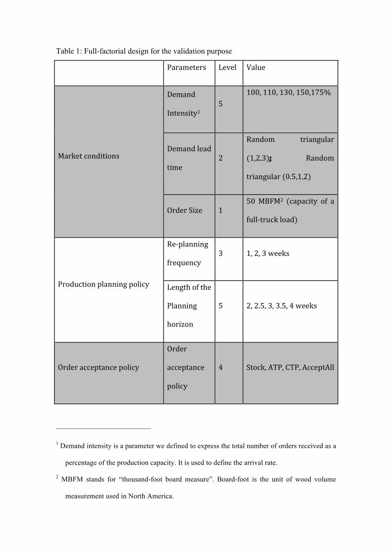
Table 1: Full-factorial design for the validation purpose
Parameters Level Value
Marketconditions
Demand
Intensity15
100,110,130,150,175%
Demandlead
time2
Random triangular
(1,2,3); Random
triangular(0.5,1,2)
OrderSize 150MBFM2 (capacity of a
full-truckload)
Productionplanningpolicy
Re-planning
frequency3 1,2,3weeks
Lengthofthe
Planning
horizon
5 2,2.5,3,3.5,4weeks
Orderacceptancepolicy
Order
acceptance
policy
4 Stock,ATP,CTP,AcceptAll
1 Demand intensity is a parameter we defined to express the total number of orders received as a
percentage of the production capacity. It is used to define the arrival rate.
2 MBFM stands for “thousand-foot board measure”. Board-foot is the unit of wood volume
measurement used in North America.

Figure 1: Conceptual representation of the model
Figure 2: Impact of the length of the planning horizon (demand intensity = 130%,
replanning frequency = 1 week)
0
10000
20000
30000
40000
50000
60000
0
20000
40000
60000
80000
100000
120000
140000
2 2,5 3 3,5 4
Averageinventory(M
BFM)
Volumeofsa
les(MBFM)
Lengthoftheplanninghorizon(weeks)
InventoryAcceptAll
InventoryATP
InventoryCTP
InventoryStock
VolumeofsalesAcceptAll
VolumeofsalesATP
VolumeofsalesCTP
VolumeofsalesStock

Figure 3: Impact of the demand intensity (length of the planning horizon = 4 weeks;
replanning frequency = 1 week)
Figure 4: Volume of sales according to the demand intensity (Commodity product =
100%; accurate forecast; length of the planning horizon = 4 weeks; replanning
frequency = 1 week)
0
2000
4000
6000
8000
10000
12000
14000
16000
18000
30000
50000
70000
90000
110000
130000
150000
100 110 130 150 175
Averageinventory(M
BFM)
Volumeofsa
les(MBFM)
Demandintensity(%ofthemaximumproductioncapacity)
InventoryAcceptAll InventoryATP InventoryCTP
InventoryStock VolumeofsalesATP VolumeofsalesCTP
VolumeofsalesStock
1200
1300
1400
1500
1600
1700
1800
1900
2000
90 140 190 240 290
Volumeofsa
les(MBFM)
Demandintensity(%ofthemaximalproductioncapacity)
VolumeofsalesATP
VolumeofsalesCTP
VolumeofsalesStock
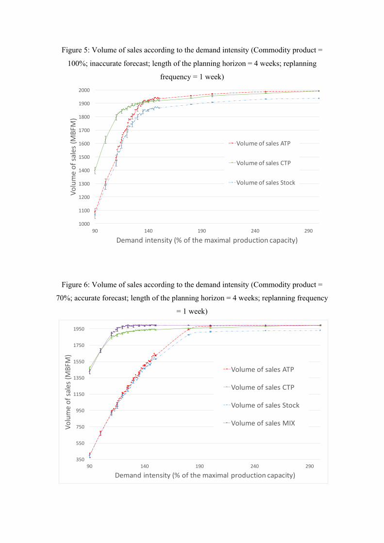
Figure 5: Volume of sales according to the demand intensity (Commodity product =
100%; inaccurate forecast; length of the planning horizon = 4 weeks; replanning
frequency = 1 week)
Figure 6: Volume of sales according to the demand intensity (Commodity product =
70%; accurate forecast; length of the planning horizon = 4 weeks; replanning frequency
= 1 week)
1000
1100
1200
1300
1400
1500
1600
1700
1800
1900
2000
90 140 190 240 290
Volumeofsa
les(MBFM)
Demandintensity(%ofthemaximalproductioncapacity)
VolumeofsalesATP
VolumeofsalesCTP
VolumeofsalesStock
350
550
750
950
1150
1350
1550
1750
1950
90 140 190 240 290
Volumeofsa
les(MBFM)
Demandintensity(%ofthemaximalproductioncapacity)
VolumeofsalesATP
VolumeofsalesCTP
VolumeofsalesStock
VolumeofsalesMIX

Figure 7: Average inventory over the year according to the demand intensity and the
associated volume of sales (Commodity product = 90%; accurate forecast; length of the
planning horizon = 4 weeks; replanning frequency = 1 week)
Figure 8: Revenues for each policy (commodity product = 70%, accurate forecasts;
length of the planning horizon = 4 weeks; replanning frequency = 1 week)
3500
5500
7500
9500
11500
13500
15500
17500
19500
21500
23500
90 140 190 240 290
Revenu
es
Demandintensity(%ofthemaximalproductioncapacity)
RevenuesATP
RevenuesCTP
RevenuesStock
RevenuesMIX

Figure 9: Decision graph taking into account the margin for a market with an accurate
forecast (length of the planning horizon = 4 weeks; replanning frequency = 1 week)