evaluating teachers and schools using student growth models · evaluating teachers and schools...

A peer-reviewed electronic journal.

Copyright is retained by the first or sole author, who grants right of first publication to the Practical Assessment, Research & Evaluation. Permission is granted to distribute this article for nonprofit, educational purposes if it is copied in its entirety and the journal is credited. PARE has the right to authorize third party reproduction of this article in print, electronic and database forms.

Volume 17, Number 17, December 2012 ISSN 1531-7714

Evaluating Teachers and Schools Using Student Growth Models

William D. Schafer, Robert W. Lissitz, Xiaoshu Zhu, Yuan Zhang, University of Maryland Xiaodong Hou, American Institutes for Research

Ying Li, American Nurses Association

Interest in Student Growth Modeling (SGM) and Value Added Modeling (VAM) arises from educators concerned with measuring the effectiveness of teaching and other school activities through changes in student performance as a companion and perhaps even an alternative to status. Several formal statistical models have been proposed for year-to-year growth and these fall into at least three clusters: simple change (e.g., differences on a vertical scale), residualized change (e.g., simple linear or quantile regression techniques), and value tables (varying salience of different achievement level outcomes across two years). Several of these methods have been implemented by states and districts. This paper reviews relevant literature and reports results of a data-based comparison of six basic SGM models that may permit aggregating across teachers or schools to provide evaluative information. Our investigation raises some issues that may compromise current efforts to implement VAM in teacher and school evaluations and makes suggestions for both practice and research based on the results.

Perhaps psychometricians should feel honored that educators, through Race to the Top (RTTT) and previously No Child Left Behind (NCLB), have turned to them in the belief that they will provide a defensible basis for tough decisions about schools and teachers. Before 2000, states or districts were generally left to develop assessment systems that satisfied their own ends (or not). Many school systems were perceived as being too slow to adopt formal approaches to evaluating the success of their enterprise and in many cases that perception had a basis in reality.

In 2001 the federal government imposed more uniform data requirements on schools with the NCLB Act. NCLB required data collections that would measure a school’s status (where students are when they finish the year, regardless of where they started). Since states were scheduled by the federal government to apply corrective actions for schools if not every student was proficient by 2014, the public seemed reassured that teachers and school

administrators would respond to the pressure to assure a quality education for all American children. However, it has become apparent that proficiency is loosely defined, and no matter how it is defined, it is more difficult to achieve for some students than for others. For these and other reasons, alternative approaches to assessing school (and teacher) effectiveness have been sought. The most popular alternative appears to be modeling growth, broadly characterized as change in student achievement from one year to the next.

About 10 years ago a number of states were approved to try some very simple change modeling. Their models are included on the web site: http://www.ed.gov/admins/lead/account/growthmodel/index.html and researchers have been examining what was proposed. Prior to any of these efforts, though, there were two jurisdictions that engaged upon comparatively sophisticated approaches to modeling student-level change for evaluating teachers and schools. One of these was

Practical Assessment, Research & Evaluation, Vol 17, No 17 Schafer, Lissitz, Zhu, Zhang, Hou & Li, Student Growth Models

an effort in Dallas, Texas. The original version of the Dallas system went into effect in 1994 and examined school effects (Webster & Mendro, 1994); this was expanded to include teacher effects in the 1995-1996 school year (Webster, Mendro, Bembry, & Orsak, 1995). The model was composed of two stages. The first stage used multiple regression to control the effects of “fairness variables,” which were defined as student differences in gender, ethnicity, English proficiency, socioeconomic status and any other variable that was considered to be an influence beyond the school’s or teacher’s ability to control. A multiple regression was used to remove these student variables by creating residual values, linearly independent of them. The second stage of the analysis used a hierarchical linear model (HLM) to control the effects of prior achievement, attendance, and school-level variables and to measure the conditional growth in student performance.

A second effort grew out of work in Tennessee (Sanders & Horn, 1994, 1998). This value-added approach, as it is sometimes called, was a great deal more statistically sophisticated. It involved a layered multiple regression model (TVAAS), that looked for the effects of teachers (and past teachers, hence the term layered) that compared student gains with their expected performance levels so they were either above or below predicted performance. Many models have been used, but the one embraced by Tennessee is a mixed effects model using longitudinal performance measures. Multiple prior years’ performance scores on several subject matter exams were used as a means of statistical control over the effects on student growth of variables correlated with teacher and school effects.

These and other Value Added Models (VAM) are intended to be a formal system that will permit the determination of the extent to which some entities (usually teachers or schools) have effected change in each student. The results are often aggregated across students so that summaries associated with each teacher (or school) are provided. In this way, evaluators hope to be able to show whether students exposed to a specific teacher (or school) are performing above or below their expected performance (or the performance levels of

students associated with other teachers or perhaps an artificial “average” teacher). Most (though not all) VAM models are inherently normative in nature.

Factors confounding teacher effects and the dynamic, interactive nature of the classroom and the school system complicate the modeling problem. Using the prior test performance to serve as a control for all sorts of other effects has been discussed by Newton, Darling-Hammond, Haertel, & Thomas (2010). Some of their analyses show a relation between change and percent minority, even after controlling for prior performance, for example. The problem, at least in part, may be that such factors are not just main effects easily controlled by recording performance levels at the beginning of the year. They interact with the teacher’s ability to be effective all year long and they interact with other student factors, as well.

Concerns about the quality of decisions based on VAM are particularly relevant where the work becomes high-stakes for teachers or schools involving dissemination, bonuses, corrective measures, or even the threat or reality of removal. A further complication to the use of VAM in teacher evaluation is that many teachers are working in areas that do not involve standardized testing. Florida (Prince, Schuermann, Guthrie, Witham, Milanowski, & Thorn, 2009, page 5), for example, has calculated that 69% of its teachers are teaching non-tested subjects and grades. In Memphis, Tennessee the current testing program does not apply to about 70% of the teachers (Lipscomb, Teh, Gill, Chiang, & Owens, 2010). This is a problem that is quite common today, although it is not the only methodological problem. For example, most teachers do not actually work alone with students. They have other teachers, other support personnel such as a librarian and counselors, plus parent volunteers, aides, and co-teachers making the assignment of attribution of effectiveness to the teacher more confused and doubtful.

Although VAM may not be ready for high-stakes decision making, perhaps it may be partnered with additional data gathering efforts to contribute to a multiple-measures view of teacher effectiveness. It seems safe to say at this juncture that VAM is


probably well worth pursuing, but is so challenging as to make high-stakes applications a very high risk.

There is clearly a need for empirical study of issues surrounding the ability of educators to draw inferences from VAM data. Our purpose here is to study the quality of VAM using data from a large suburban school district. We will discuss issues surrounding reliability and then validity as applied to VAM and then explore some of the more salient concerns using actual data.

Reliability

If one thinks of the reliability of VAM in the context of generalizability, we can ask if effectiveness estimates for teachers (or perhaps schools) are stable across changes in when a test is given, which test is administered, what course the teacher is responsible for, and what grade the students are enrolled in, to name just a few relevant facets. If we want to characterize one teacher as effective and another as ineffective, we need to be concerned with whether such a characterization is justified independent of context, or whether teachers are actually more effective in some circumstances and less effective in others. The following comments are a very brief summary of some results from relevant literature.

Stability over a one-year period: In an early study, Mandeville (1988) explored the estimation of effectiveness as a school residual from the expectation of a regression model across consecutive years. He found that school residual correlations were stable only in the 0.34 to 0.66 range, a disappointing finding for an outcome based upon an entire school.

McCaffrey, Koretz, Lockwood, & Milhaly (2009) also found low stability, this time at the teacher level. They report correlations in the 0.2 to 0.3 range for a one-year interval. Others who have looked at this form of the reliability question include Newton, et al. (2010) and Corcoran (2010), with similar results.

We certainly know that there are many sources of unreliability that can negatively impact the stability of characterizations of individual teachers. Test reliability is just one source. McCaffrey et al.

(2009) make a very useful distinction between the reliability of teacher characterizations across a year in time and the reliability of the measures themselves.

It is not clear that teaching performance itself can be considered a stable phenomenon. That is, teacher effects may be at least partly a function of an interaction with the nature of the students and changes in the teachers themselves. If the instability is due to sampling error or some statistical issues, at least it might be reduced by increasing sample size and averaging. If the variability is due to actual performance changes from year to year, then the problem may be intractable (McCaffrey, et al. 2009).

Stability over a short period of time: Sass (2008) and Newton, et al. (2010) found that estimates of teacher effectiveness defined from what amounts to test-retest assessments over a very short time period were reasonably high. Correlations in the range of 0.6, for example, have been reported in the literature. This shows that teacher effectiveness may be somewhat consistent if we look the second time shortly after our first view of the teacher. We usually demand greater reliability for high stakes testing, so these results should cause us some alarm, but they do seem to indicate that something real is occurring.

Stability across grade and subject: Mandeville and Anderson (1987) and others (e.g. Rockoff, 2004; Newton, et al., 2010) found that stability fluctuated across grade and subject matter. Though limited, stability was greater for mathematics courses than for reading courses, raising issues of fairness and comparability across content as well as class assignments at the teacher level.

Stability across test forms: Sass (2008) compared performance quintiles and found that the top 20% and the bottom 20% seemed to be the most stable based on both a low-stakes and a high-stakes exam. The correlation of teacher effectiveness for these data was 0.48 across comparable examinations. Note that this correlation was based on two different, but somewhat related exams over a short time period and limited to classification of teachers into five


quality categories (quintiles). When the time period was extended to a year’s duration between tests, the correlation of teacher effectiveness dropped to 0.27.

Papay (2011) also looked at the issue of stability across test forms and explored VAM estimates using three different tests. Rank order correlations of teacher effectiveness across time ranged from 0.15 to 0.58 across the different tests. Test timing and measurement error were credited with causing some of the relatively low levels of stability of the teacher effect sizes.

Stability across statistical models: Linear composites in general tend to perform similarly regardless of how one gets the weights (Dawes, 1979). Tekwe, Carter, Ma, Algina, Lucas, & Roth (2004) compared four regression models and found that unless the models involve different variables, the results tend to be quite similar. Three of the models gave consistent results; another model involving variables not included in the others (poverty and minority status) resulted in somewhat different estimates of effectiveness. Hill, Kapitula, & Umland (2011) discuss this as a convergent validity problem.

Stability across Classrooms: Newton, et al. (2010) looked at factors that affect teacher effectiveness and found that stability of teacher ratings can vary as a function of classes taught. They also found that teaching students who are less advantaged, ESL, in a lower track, and/or low income students can have a negative impact on teacher effectiveness estimates. In many cases they even found inverse relationships among courses taught by the same teacher, although these results were generally not significant. Their study also tried to match VAM scores with extensive information about teaching ability. Multiple VAM models were used, and the success of matching teacher characteristics to VAM outcomes was judged to be modest. It is tempting to consider the VAM score as a criterion to be used to judge other variables, but their questionable validity (see below) makes that a doubtful approach.

The effort to develop a fair and equitable system for scoring two teachers with the same teaching skills, despite teaching two different groups

of students (perhaps one with language challenged and learning disabled students and the other not) is certainly a worthy goal. Will we find stability, or fairness to be present in such a system? At this point we do not appear to have models that are so accurate that they can ignore or compensate for the context of the instruction. Indeed, it may be doubtful that effective teaching is a simple construct that is independent of the characteristics of the students or the context of the classroom.

Summary: We seem to know that effectiveness is not very highly correlated with itself over a one-year period, across different tests, across different subject matter or across different grades. Glazerman, Loeb, Goldhaber, Staiger, Raudenbush, and Whitehurst (2010) briefly summarized similar stability indices for various different occupations and found that the lack of consistency observed for teachers is not unusual. When compared to baseball players, stock investors, and several other complex professions, we find comparably low reliability. They concluded that while teacher effectiveness does not seem to correlate from year to year particularly well, teachers are no less reliable than other professionals working in complex industries. Perhaps the trait of effectiveness is not very stable in the first place, apart from its assessment.

Validity

Validity is a much more complex concept than reliability and it is not altogether clear how we should verify the validity of work on teacher or school effectiveness. We will begin by a review of correlates of VAM results at the teacher level.

Job applications as measures predicting effectiveness: It would be useful to find that there are associations between teacher effects and the typical information associated with a teacher’s application for employment. Unfortunately, while some evidence for the utility of such factors exists, they are, at best, weak as indicators. Consistent with an early study by Hanushek (1986), Sass (2008) noted that such variables as years of experience and advanced degrees have low relationships, if any, to teacher effectiveness. Sanders, Ashton, and Wright (2005) did find a weak relationship between effectiveness and possession of an advanced degree,


but this result was described in a later paper as little better than a coin flip between teachers with National Board for Professional Teaching Standards certification and those without (Sanders and Wright, 2008). Goldhaber and Hanson (2010) found with North Carolina data that VAM estimates seem to provide better measures of teacher impact on student test scores than do measures obtained at the time a teacher applies for employment. They included such measures as degree, experience, possessing a master’s degree, college selectivity, and licensure in addition to VAM estimated teacher effects.

Hill, Kapitula & Umland (2011) in a study of mathematics teachers, found that knowledge of mathematics was positively correlated with effectiveness. They found that VAM scores correlate with math knowledge and the characteristics of the students they are teaching. But even this association was weak.

Triangulation of multiple indicators: Goe, Bell and Little (2008) discuss other ways of evaluating teachers, specifically using some form of observation and identifying the factors that lead to effectiveness. They reference Danielson’s (1996) Framework for Teaching as a common source for collecting relevant information about teachers. One implication, as Goe et al. (2008) say, is that teachers should be compared to other teachers who teach similar courses in the same grade in a similar context and assessed by the same or similar examination. That is certainly consistent with the literature on VAM stability, referenced above, and what is probably necessary to eventually establish validity. It also acknowledges the complex interactions that seem to exist.

Comparability: It is often assumed that initial status is actually independent or at least uncorrelated with change, and some models force nonassociation (e.g., regression models). As Kupermintz (2003) suggests, though, ability is more likely to be correlated with growth and status. Indeed, Kupermintz (2003) notes there may also be an interaction between student ability and the ability of teachers to exhibit their effectiveness. The estimation of teacher effects seems to present us

with a very complex interaction involving mixtures of students and teachers.

Summary. As with reliability, the validity of inferences made from VAM outcomes seems weak. We do not find correlates at the teacher level that are useful in practice and correlations at the student level may only serve to further compromise teacher assessment using VAM. Perhaps as Rubin, Stuart, & Zanutto (2004) suggested, a theory of student instruction that involves teacher effectiveness constructs is needed. Without a theory it is hard to determine just how we would validate teacher or school effectiveness and their associated causality, if in fact there is any.

Unresolved Issues.

Interest on the part of educators to explore alternatives to status measures as a way to document school success has led state and federal agencies to encourage aggregates of student change as a possible way to assess the quality of teachers and schools. However, there is very little empirical research that supports the effectiveness of change measures on the psychometric criteria of reliability and validity at any level of aggregation. Exploration of change measures with real data would not only be helpful for applied researchers in educational outcomes assessment; it is urgent in a political climate that encourages decision making based on change. Our goal here is to provide an empirical investigation of the reliability and validity of growth measure alternatives for students, and especially for teachers and schools, where inferences are most often drawn.

STUDY DESIGN

For the present study, we used in their most basic forms, six change model formulations that have been suggested in the literature. We used data from several years that were made available to us by a large suburban county in the eastern United States. We explored reliability at all three levels of aggregation along with validity evidence based on correlations with available traits. This article is drawn and gives examples from a larger study undertaken by the Maryland Assessment Research Center for Education Success at the University of Maryland (MARCES, 2012); the full report along


with further background information and all analyses is available at: marces.org/completed.htm.

Data Source

The data made available to us were three years (2008, 2009, 2010) of reading and math scores on the regular statewide achievement tests for 3rd through 8th grade students along with the students’ schools and teachers. Since some of the models we studied involved three years of data, we considered these data to consist of four cohorts, (1) grades 3 through 5, (2) grades 4 through 6, (3) grades 5 through 7 and (4) grades 6 through 8.

The data we used are from public schools in a large, suburban county. There were 107 elementary schools and 28 middle schools represented (all the schools of these types in the county). Overall, the district is (2011 data) 45.94% white, 38.74% African-American, 6.00% Asian, 5.92%

Hispanic/Latino, and 3.40% other or mixed races. Over the three years in our study, county-wide grade cohorts in the grades studied varied from a low of 7,258 to a high of 7,845, The percentages of these grade-level student populations who were eligible for free or reduced-price meals ranged between 35.85 and 45.35. Across these populations, the percentages classified as limited-English proficient ranged from 0.86 to 4.51 and the percentages identified as special education ranged from 9.91 to 12.61.

We received data for all students in the four cohorts in the district who took the regular state assessments. The alpha coefficients of these tests ranged from .93 to .95 in math and from .82 to .88 in reading. In our pre-processing of the data file, we decided to restrict our work to those students who did not present issues such as missing data that would require compromises to a straightforward model implementation. We thus deleted students without all three math and all three reading scores and who had been assigned to multiple reading or math teachers in any one year. At that point we treated the cohorts and contents separately (eight groups) and deleted cases when there were fewer than 5 in any one classroom or 25 in any one school. We created a teacher database and a school database by aggregating students to each level. This process resulted in the sample sizes shown in Table 1.

Neither the reading nor the math assessment is vertically scaled, although each is linked to a comparable grade-content base year test’s scale that has been in existence for several years. The lack of a vertical scale prompted us to examine six simple models that do not require vertical linking from year to year (though one of them utilizes an alternative to a vertical scale). These six models were used to characterize change from the first year to the second for each student across two years in each cohort. For some analyses, two additional models were used

Table 1. Sample Size at Each Level Math Reading

Year Level Cohort1 Cohort2 Cohort3 Cohort4 Cohort1 Cohort2 Cohort3 Cohort4

2008-2009

Student 5689 5536 5567 5791 5610 4803 4757 5075Teacher 292 262 96 120 268 107 122 122School 103 102 27 28 103 100 27 27

2009-2010

Student 5706 5541 5537 5756 5625 4897 4737 5093

Teacher 306 283 94 103 291 91 97 95

School 103 27 27 28 103 27 27 27

Notes: Cohort 1 were 3rd through 5th graders in 2008-2010. Cohort 2 were 4th through 6th graders in 2008-2010. Cohort 3 were 5th through 7th graders in 2008-2010. Cohort 4 were 6th through 8th graders in 2008-2010.


to model change from the first and second years (two predictors) to the third in order to evaluate the usefulness of more than one year of prior information.

Models

Here we describe the resulting eight models more completely. The acronyms we used are bolded within the text. A complete list of the major acronyms along with brief characterizations is given later in Table 5.

Betebenner’s model (Betebenner 2008, 2012) is quite popular, currently being used in Colorado, for example. It uses quantile regression to estimate the conditional percentile of each student’s performance in the second year compared to other students who started at the identical percentile in the initial year. The student’s change score is an estimate of the percentile in year two within the group of students with the identical percentile in year one. Aggregating these differences for a teacher (or school or other grouping) gives a value added measure for that teacher (or school. etc.). (We use the term “growth score” later in a more specialized way and in order to avoid confusion we use the term “change score” to refer to a VAM result here and throughout the rest of the paper.)

We looked at two models that used this approach. One used the prior year only as the predictor (QReg1) and the second used both prior years (QReg2) to condition the percentile in the third year.

Thum (2003) uses an effect size rather than a percentile. It amounts to a z score that identifies a student’s performance level in the second year compared to the average student scoring at the student’s level in the first year. As with the Betebenner model, change is measured as movement of students relative to students who started out at conditionally the same position. Although Thum’s model can condition on additional variables as well, we have used only the prior year’s score in order to make the comparisons among the methods more equivalent. In order to simplify the procedure, we implemented a model similar in concept to Thum’s, but using ordinary least squares (OLS) as opposed to maximum

likelihood regression estimates. In other words, we used traditional statistical estimation methods to find student residuals around a regression equation. We implemented OLS with the prior year as the only predictor (OLS1) and with two prior years as predictors (OLS2) to parallel our Betebenner model applications.

The above models are entirely norm-based. The mean change for each of them is arbitrary and thus an average overall increase (or decrease) from one year to the next is not reflected in the results. The remaining four models, however, can be influenced by overall positive (or negative) change.

As we noted, we did not have a vertical scale. Instead, growth (spline) scores (Schafer& Hou, 2011) were used to study the behavior of outcomes similar to those that might result from a vertical scale. The growth scores were based on look-up tables derived from an earlier study using statewide data for each test (Schafer, Hou, & Lissitz, 2009). Each table was developed as a spline function created to give moderated (consistent) meaning to various points along the performance continuum across grades and contents, scaled using 2008 data. The spline functions were essentially piecewise curve fitting models used to rescale the data. The transformations were matched to cut scores for five moderated proficiency levels related to existing statewide interpretations of the levels. The resulting quasi-vertical scales, constructed without using common items, are linear transforms of what has been called a growth scale that for some purposes actually may be superior to a vertical scale (Schafer, 2006). Once we had consistently-scaled scores, we subtracted the growth (spline) score at the earlier grade (pretest) from the growth (spline) score at the later grade (posttest), as though they were from a true vertical scale (DifGr).

Transition models (also called value tables; see Hill, R., Gong, B., Marion, S., DePascal, C., Dunn, J, & Simpson, M., 2005) were applied with one adapted from an existing use in Delaware, a second that adapts an existing use in Arkansas, and a third suggested by Schafer (2007, 2008) that is used in Maryland. These models all start with the classification of students into categories based on statewide definitions of basic, proficient and


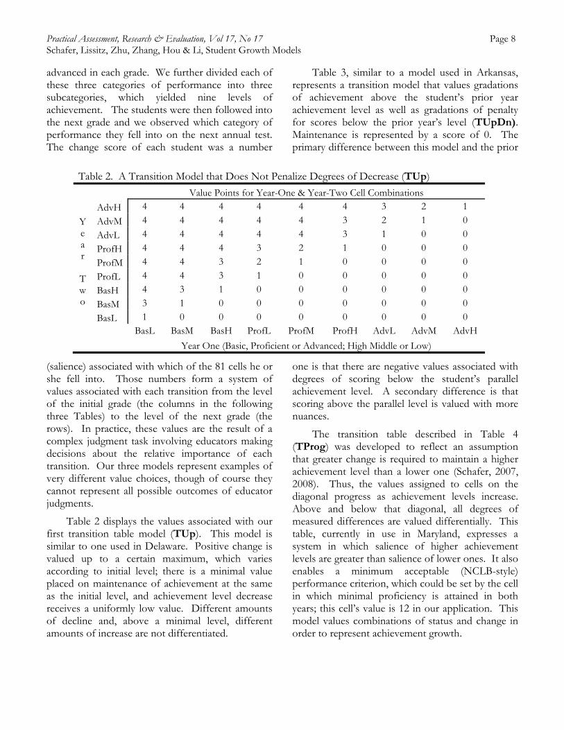
advanced in each grade. We further divided each of these three categories of performance into three subcategories, which yielded nine levels of achievement. The students were then followed into the next grade and we observed which category of performance they fell into on the next annual test. The change score of each student was a number

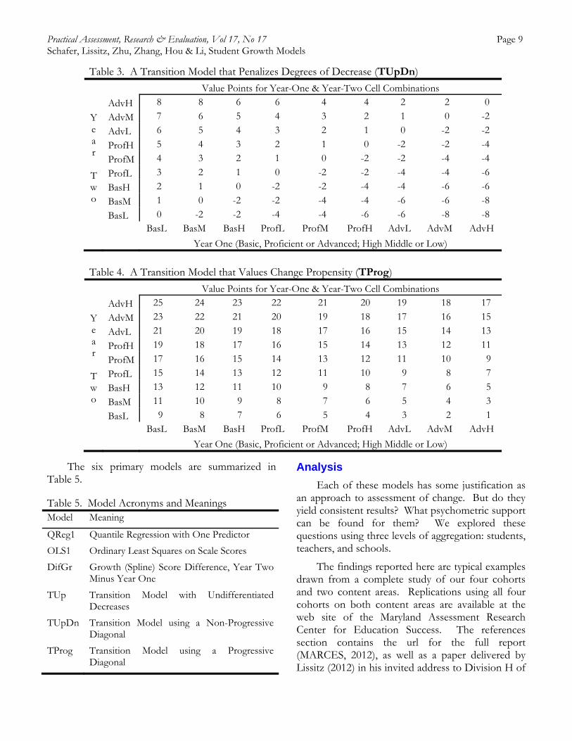
(salience) associated with which of the 81 cells he or she fell into. Those numbers form a system of values associated with each transition from the level of the initial grade (the columns in the following three Tables) to the level of the next grade (the rows). In practice, these values are the result of a complex judgment task involving educators making decisions about the relative importance of each transition. Our three models represent examples of very different value choices, though of course they cannot represent all possible outcomes of educator judgments.

Table 2 displays the values associated with our first transition table model (TUp). This model is similar to one used in Delaware. Positive change is valued up to a certain maximum, which varies according to initial level; there is a minimal value placed on maintenance of achievement at the same as the initial level, and achievement level decrease receives a uniformly low value. Different amounts of decline and, above a minimal level, different amounts of increase are not differentiated.

Table 3, similar to a model used in Arkansas, represents a transition model that values gradations of achievement above the student’s prior year achievement level as well as gradations of penalty for scores below the prior year’s level (TUpDn). Maintenance is represented by a score of 0. The primary difference between this model and the prior

one is that there are negative values associated with degrees of scoring below the student’s parallel achievement level. A secondary difference is that scoring above the parallel level is valued with more nuances.

The transition table described in Table 4 (TProg) was developed to reflect an assumption that greater change is required to maintain a higher achievement level than a lower one (Schafer, 2007, 2008). Thus, the values assigned to cells on the diagonal progress as achievement levels increase. Above and below that diagonal, all degrees of measured differences are valued differentially. This table, currently in use in Maryland, expresses a system in which salience of higher achievement levels are greater than salience of lower ones. It also enables a minimum acceptable (NCLB-style) performance criterion, which could be set by the cell in which minimal proficiency is attained in both years; this cell’s value is 12 in our application. This model values combinations of status and change in order to represent achievement growth.

Table 2. A Transition Model that Does Not Penalize Degrees of Decrease (TUp)

Value Points for Year-One & Year-Two Cell Combinations

Y e a r

T w o

AdvH 4 4 4 4 4 4 3 2 1

AdvM 4 4 4 4 4 3 2 1 0

AdvL 4 4 4 4 4 3 1 0 0

ProfH 4 4 4 3 2 1 0 0 0

ProfM 4 4 3 2 1 0 0 0 0

ProfL 4 4 3 1 0 0 0 0 0

BasH 4 3 1 0 0 0 0 0 0

BasM 3 1 0 0 0 0 0 0 0

BasL 1 0 0 0 0 0 0 0 0

BasL BasM BasH ProfL ProfM ProfH AdvL AdvM AdvH

Year One (Basic, Proficient or Advanced; High Middle or Low)


The six primary models are summarized in Table 5.

Table 5. Model Acronyms and Meanings Model Meaning

QReg1 Quantile Regression with One Predictor

OLS1 Ordinary Least Squares on Scale Scores

DifGr Growth (Spline) Score Difference, Year Two Minus Year One

TUp Transition Model with Undifferentiated Decreases

TUpDn Transition Model using a Non-Progressive Diagonal

TProg Transition Model using a Progressive Diagonal

Analysis

Each of these models has some justification as an approach to assessment of change. But do they yield consistent results? What psychometric support can be found for them? We explored these questions using three levels of aggregation: students, teachers, and schools.

The findings reported here are typical examples drawn from a complete study of our four cohorts and two content areas. Replications using all four cohorts on both content areas are available at the web site of the Maryland Assessment Research Center for Education Success. The references section contains the url for the full report (MARCES, 2012), as well as a paper delivered by Lissitz (2012) in his invited address to Division H of

Table 3. A Transition Model that Penalizes Degrees of Decrease (TUpDn)


Y e a r

T w o

AdvH 8 8 6 6 4 4 2 2 0

AdvM 7 6 5 4 3 2 1 0 -2

AdvL 6 5 4 3 2 1 0 -2 -2

ProfH 5 4 3 2 1 0 -2 -2 -4

ProfM 4 3 2 1 0 -2 -2 -4 -4

ProfL 3 2 1 0 -2 -2 -4 -4 -6

BasH 2 1 0 -2 -2 -4 -4 -6 -6

BasM 1 0 -2 -2 -4 -4 -6 -6 -8

BasL 0 -2 -2 -4 -4 -6 -6 -8 -8



Table 4. A Transition Model that Values Change Propensity (TProg)


Y e a r

T w o

AdvH 25 24 23 22 21 20 19 18 17

AdvM 23 22 21 20 19 18 17 16 15

AdvL 21 20 19 18 17 16 15 14 13

ProfH 19 18 17 16 15 14 13 12 11

ProfM 17 16 15 14 13 12 11 10 9

ProfL 15 14 13 12 11 10 9 8 7

BasH 13 12 11 10 9 8 7 6 5

BasM 11 10 9 8 7 6 5 4 3

BasL 9 8 7 6 5 4 3 2 1




the American Educational Research Association and that was based on the same dataset.

The results are presented first by exploring whether there are differences among the six primary models in the ways they describe change. This was studied at the student and teacher levels through examining the inter-correlations among the measures. Strong correlations should indicate that the measures are focusing on similar constructs. Our second set of analyses was designed to evaluate the consistencies (reliabilities) of the change measures across years at the student, teacher, and school levels. If change is to be used as an element in program or personnel evaluation, then as a rule of thumb we would expect to find reliabilities in .7 or higher range. Third, we looked at whether the change scores in reading are associated with the change scores in math; moderately high correlations would yield convergent evidence of validity. Finally, we examined relationships among the change scores and other variables, including absolute achievement (criterion-related validity evidence; correlations with posttest should be reasonably high, but it is unclear what expectations should be for correlations with pretests, near zero or moderately positive), demographics (moderately low correlations would provide divergent evidence of validity) and grade levels (low correlations would suggest fairness).

1. Inter-correlations of Change Scores

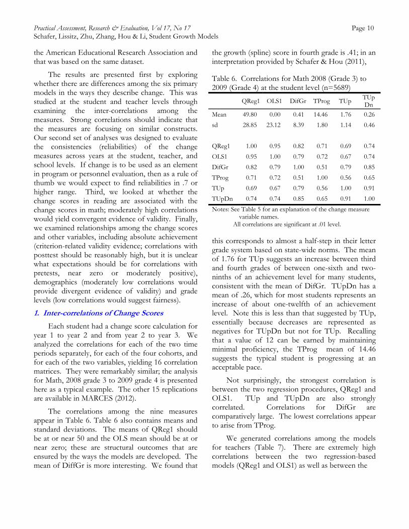
Each student had a change score calculation for year 1 to year 2 and from year 2 to year 3. We analyzed the correlations for each of the two time periods separately, for each of the four cohorts, and for each of the two variables, yielding 16 correlation matrices. They were remarkably similar; the analysis for Math, 2008 grade 3 to 2009 grade 4 is presented here as a typical example. The other 15 replications are available in MARCES (2012).

The correlations among the nine measures appear in Table 6. Table 6 also contains means and standard deviations. The means of QReg1 should be at or near 50 and the OLS mean should be at or near zero; these are structural outcomes that are ensured by the ways the models are developed. The mean of DiffGr is more interesting. We found that

the growth (spline) score in fourth grade is .41; in an interpretation provided by Schafer & Hou (2011),

Table 6. Correlations for Math 2008 (Grade 3) to 2009 (Grade 4) at the student level (n=5689)

QReg1 OLS1 DifGr TProg TUp TUpDn

Mean 49.80 0.00 0.41 14.46 1.76 0.26

sd 28.85 23.12 8.39 1.80 1.14 0.46

QReg1 1.00 0.95 0.82 0.71 0.69 0.74

OLS1 0.95 1.00 0.79 0.72 0.67 0.74

DifGr 0.82 0.79 1.00 0.51 0.79 0.85

TProg 0.71 0.72 0.51 1.00 0.56 0.65

TUp 0.69 0.67 0.79 0.56 1.00 0.91

TUpDn 0.74 0.74 0.85 0.65 0.91 1.00

Notes: See Table 5 for an explanation of the change measure variable names.

All correlations are significant at .01 level. this corresponds to almost a half-step in their letter grade system based on state-wide norms. The mean of 1.76 for TUp suggests an increase between third and fourth grades of between one-sixth and two-ninths of an achievement level for many students, consistent with the mean of DifGr. TUpDn has a mean of .26, which for most students represents an increase of about one-twelfth of an achievement level. Note this is less than that suggested by TUp, essentially because decreases are represented as negatives for TUpDn but not for TUp. Recalling that a value of 12 can be earned by maintaining minimal proficiency, the TProg mean of 14.46 suggests the typical student is progressing at an acceptable pace.

Not surprisingly, the strongest correlation is between the two regression procedures, QReg1 and OLS1. TUp and TUpDn are also strongly correlated. Correlations for DifGr are comparatively large. The lowest correlations appear to arise from TProg.

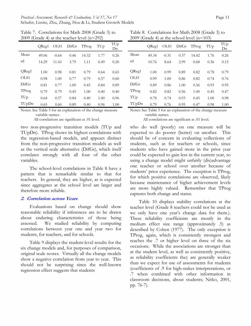
We generated correlations among the models for teachers (Table 7). There are extremely high correlations between the two regression-based models (QReg1 and OLS1) as well as between the


Table 7. Correlations for Math 2008 (Grade 3) to 2009 (Grade 4) at the teacher level (n=292)


Mean 49.06 -0.64 0.46 14.32 1.77 0.26 sd 14.29 11.43 3.79 1.11 0.49 0.20

QReg1 1.00 0.98 0.81 0.79 0.64 0.65 OLS1 0.98 1.00 0.77 0.79 0.57 0.60 DifGr 0.81 0.77 1.00 0.45 0.84 0.89 TProg 0.79 0.79 0.45 1.00 0.40 0.40 TUp 0.64 0.57 0.84 0.40 1.00 0.96 TUpDn 0.65 0.60 0.89 0.40 0.96 1.00 Notes: See Table 5 for an explanation of the change measure

variable names. All correlations are significant at .01 level.

two non-progressive transition models (TUp and TUpDn). TProg shows its highest correlations with the regression-based models, and appears distinct from the non-progressive transition models as well as the vertical scale alternative (DifGr), which itself correlates strongly with all four of the other variables.

The school-level correlations in Table 8 have a pattern that is remarkable similar to that for teachers. In general, they are higher, as is expected since aggregates at the school level are larger and therefore more reliable.

2. Correlation across Years

Evaluations based on change should show reasonable reliability if inferences are to be drawn about enduring characteristics of those being assessed. We studied reliability by computing correlations between year one and year two for students, for teachers, and for schools.

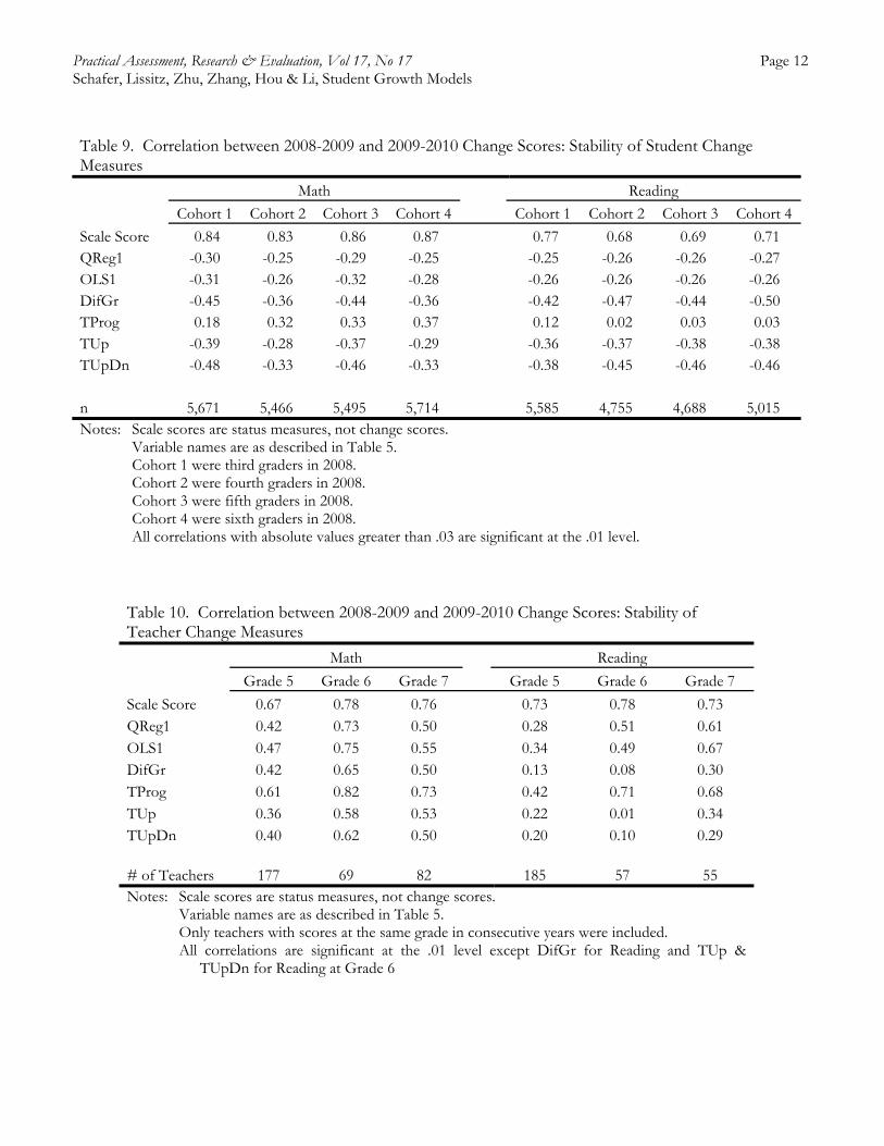
Table 9 displays the student-level results for the six change models and, for purposes of comparison, original scale scores. Virtually all the change models show a negative correlation from year to year. This should not be surprising since the well-known regression effect suggests that students

Table 8. Correlations for Math 2008 (Grade 3) to 2009 (Grade 4) at the school level (n=103)


Mean 49.34 -0.31 0.37 14.42 1.76 0.26 sd 10.76 8.64 2.99 0.68 0.36 0.15

QReg1 1.00 0.99 0.89 0.82 0.78 0.79 OLS1 0.99 1.00 0.86 0.82 0.74 0.76 DifGr 0.89 0.86 1.00 0.56 0.93 0.95 TProg 0.82 0.82 0.56 1.00 0.45 0.47 TUp 0.78 0.74 0.93 0.45 1.00 0.98 TUpDn 0.79 0.76 0.95 0.47 0.98 1.00 Notes: See Table 5 for an explanation of the change measure

variable names. All correlations are significant at .01 level.

who do well (poorly) on one measure will be expected to do poorer (better) on another. This should be of concern in evaluating collections of students, such as for teachers or schools, since students who have gained more in the prior year could be expected to gain less in the current year, so using a change model might unfairly (dis)advantage one teacher or school over another because of students’ prior experience. The exception is TProg, for which positive correlations are observed, likely because maintenance of higher achievement levels are more highly valued. Remember that TProg captures both change and status.

Table 10 displays stability correlations at the teacher level (Grade 8 teachers could not be used as we only have one year’s change data for them.). These reliability coefficients are mostly in the medium effect size range (approximately .5) as described by Cohen (1977). The only exception is TProg, again, which is consistently strongest and reaches the .7 or higher level on three of the six occasions. While the associations are stronger than at the student level, as well as consistently positive, as reliability coefficients they are generally weaker than we expect for use of assessments for students (coefficients of .9 for high-stakes interpretations, or .7 when combined with other information in classroom decisions, about students; Nitko, 2001, pp. 76-7).


Table 9. Correlation between 2008-2009 and 2009-2010 Change Scores: Stability of Student Change Measures Math Reading Cohort 1 Cohort 2 Cohort 3 Cohort 4 Cohort 1 Cohort 2 Cohort 3 Cohort 4

Scale Score 0.84 0.83 0.86 0.87 0.77 0.68 0.69 0.71 QReg1 -0.30 -0.25 -0.29 -0.25 -0.25 -0.26 -0.26 -0.27 OLS1 -0.31 -0.26 -0.32 -0.28 -0.26 -0.26 -0.26 -0.26 DifGr -0.45 -0.36 -0.44 -0.36 -0.42 -0.47 -0.44 -0.50 TProg 0.18 0.32 0.33 0.37 0.12 0.02 0.03 0.03 TUp -0.39 -0.28 -0.37 -0.29 -0.36 -0.37 -0.38 -0.38 TUpDn -0.48 -0.33 -0.46 -0.33 -0.38 -0.45 -0.46 -0.46 n 5,671 5,466 5,495 5,714 5,585 4,755 4,688 5,015 Notes: Scale scores are status measures, not change scores. Variable names are as described in Table 5. Cohort 1 were third graders in 2008. Cohort 2 were fourth graders in 2008. Cohort 3 were fifth graders in 2008. Cohort 4 were sixth graders in 2008. All correlations with absolute values greater than .03 are significant at the .01 level.

Table 10. Correlation between 2008-2009 and 2009-2010 Change Scores: Stability of Teacher Change Measures

Math

Reading

Grade 5 Grade 6 Grade 7 Grade 5 Grade 6 Grade 7

Scale Score 0.67 0.78 0.76 0.73 0.78 0.73 QReg1 0.42 0.73 0.50 0.28 0.51 0.61 OLS1 0.47 0.75 0.55 0.34 0.49 0.67 DifGr 0.42 0.65 0.50 0.13 0.08 0.30 TProg 0.61 0.82 0.73 0.42 0.71 0.68 TUp 0.36 0.58 0.53 0.22 0.01 0.34 TUpDn 0.40 0.62 0.50 0.20 0.10 0.29 # of Teachers 177 69 82 185 57 55 Notes: Scale scores are status measures, not change scores. Variable names are as described in Table 5. Only teachers with scores at the same grade in consecutive years were included.

All correlations are significant at the .01 level except DifGr for Reading and TUp & TUpDn for Reading at Grade 6


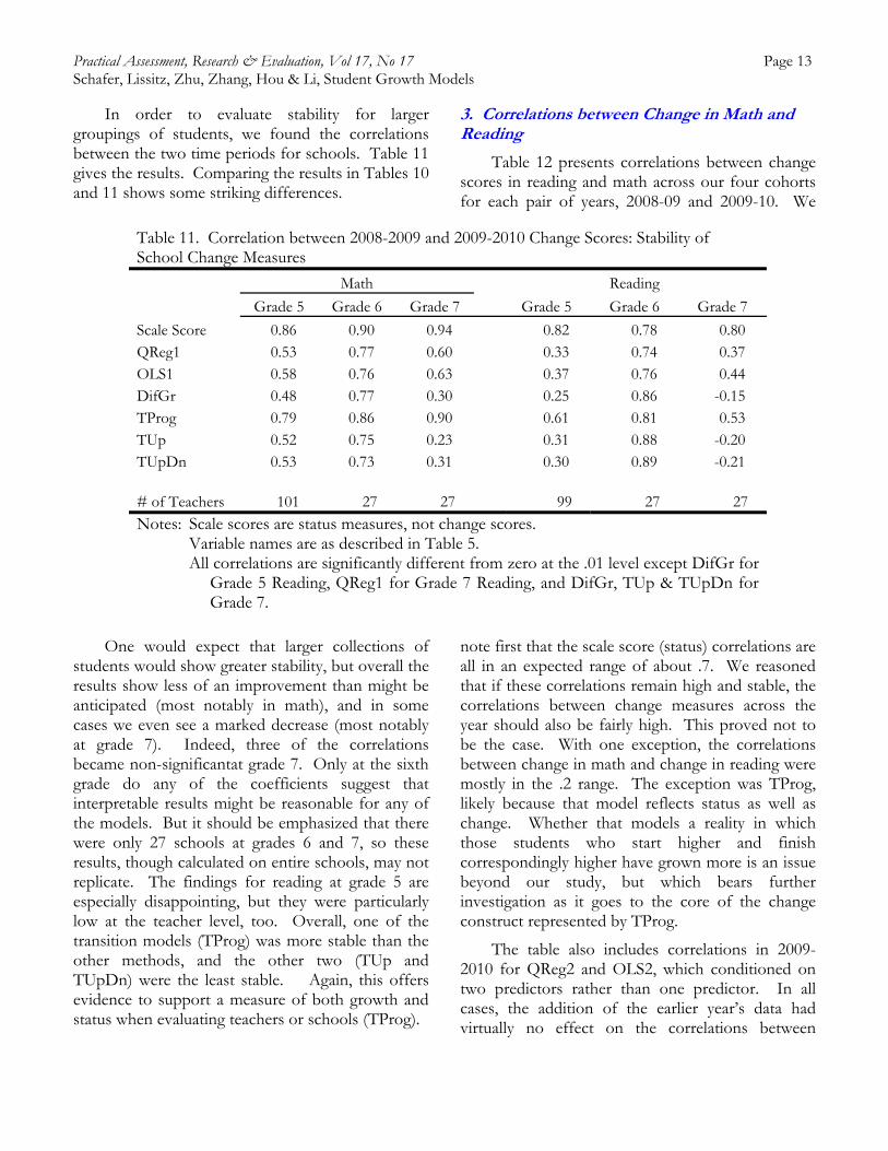
In order to evaluate stability for larger groupings of students, we found the correlations between the two time periods for schools. Table 11 gives the results. Comparing the results in Tables 10 and 11 shows some striking differences.

One would expect that larger collections of students would show greater stability, but overall the results show less of an improvement than might be anticipated (most notably in math), and in some cases we even see a marked decrease (most notably at grade 7). Indeed, three of the correlations became non-significantat grade 7. Only at the sixth grade do any of the coefficients suggest that interpretable results might be reasonable for any of the models. But it should be emphasized that there were only 27 schools at grades 6 and 7, so these results, though calculated on entire schools, may not replicate. The findings for reading at grade 5 are especially disappointing, but they were particularly low at the teacher level, too. Overall, one of the transition models (TProg) was more stable than the other methods, and the other two (TUp and TUpDn) were the least stable. Again, this offers evidence to support a measure of both growth and status when evaluating teachers or schools (TProg).

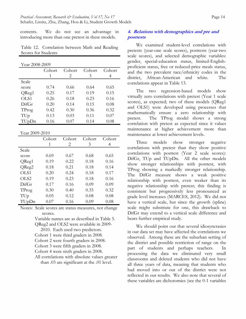
3. Correlations between Change in Math and Reading

Table 12 presents correlations between change scores in reading and math across our four cohorts for each pair of years, 2008-09 and 2009-10. We

note first that the scale score (status) correlations are all in an expected range of about .7. We reasoned that if these correlations remain high and stable, the correlations between change measures across the year should also be fairly high. This proved not to be the case. With one exception, the correlations between change in math and change in reading were mostly in the .2 range. The exception was TProg, likely because that model reflects status as well as change. Whether that models a reality in which those students who start higher and finish correspondingly higher have grown more is an issue beyond our study, but which bears further investigation as it goes to the core of the change construct represented by TProg.

The table also includes correlations in 2009-2010 for QReg2 and OLS2, which conditioned on two predictors rather than one predictor. In all cases, the addition of the earlier year’s data had virtually no effect on the correlations between

Table 11. Correlation between 2008-2009 and 2009-2010 Change Scores: Stability of School Change Measures

Math

Reading

Grade 5 Grade 6 Grade 7 Grade 5 Grade 6 Grade 7

Scale Score 0.86 0.90 0.94 0.82 0.78 0.80 QReg1 0.53 0.77 0.60 0.33 0.74 0.37 OLS1 0.58 0.76 0.63 0.37 0.76 0.44 DifGr 0.48 0.77 0.30 0.25 0.86 -0.15 TProg 0.79 0.86 0.90 0.61 0.81 0.53 TUp 0.52 0.75 0.23 0.31 0.88 -0.20 TUpDn 0.53 0.73 0.31 0.30 0.89 -0.21 # of Teachers 101 27 27 99 27 27

Notes: Scale scores are status measures, not change scores. Variable names are as described in Table 5.

All correlations are significantly different from zero at the .01 level except DifGr for Grade 5 Reading, QReg1 for Grade 7 Reading, and DifGr, TUp & TUpDn for Grade 7.


contents. We do not see an advantage in introducing more than one pretest in these models.

Table 12. Correlation between Math and Reading Scores for Students Year 2008-2009

Cohort

1 Cohort

2 Cohort

3 Cohort

4 Scale score 0.74 0.66 0.64 0.65 QReg1 0.25 0.17 0.19 0.15 OLS1 0.26 0.18 0.23 0.16 DifGr 0.20 0.14 0.15 0.08 TProg 0.42 0.30 0.36 0.32 TUp 0.13 0.03 0.11 0.07 TUpDn 0.16 0.07 0.14 0.08 Year 2009-2010

Cohort

1 Cohort

2 Cohort

3 Cohort

4 Scale score 0.69 0.67 0.68 0.65 QReg1 0.19 0.22 0.18 0.16 QReg2 0.18 0.21 0.18 0.14 OLS1 0.20 0.24 0.18 0.17 OLS2 0.19 0.23 0.18 0.16 DifGr 0.17 0.16 0.09 0.09 TProg 0.30 0.40 0.35 0.32 TUp 0.05 0.12 0.08 0.08 TUpDn 0.07 0.16 0.09 0.08 Notes: Scale scores are status measures, not change

scores. Variable names are as described in Table 5. QReg2 and OLS2 were available in 2009-

2010. Each used two predictors. Cohort 1 were third graders in 2008. Cohort 2 were fourth graders in 2008. Cohort 3 were fifth graders in 2008. Cohort 4 were sixth graders in 2008. All correlations with absolute values greater

than .03 are significant at the .01 level.

4. Relations with demographics and pre and posttests

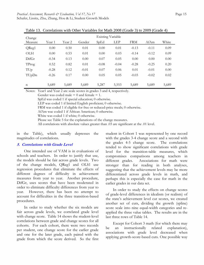
We examined student-level correlations with pretests (year-one scale scores), posttests (year-two scale scores), and selected demographic variables: gender, special-education status, limited-English-proficient status, free or reduced-price meals status, and the two prevalent race/ethnicity codes in the district, African-American and white. The correlations appear in Table 13.

The two regression-based models show virtually zero correlations with pretest (Year 1 scale scores), as expected; two of these models (QReg1 and OLS1) were developed using processes that mathematically ensure a zero relationship with pretest. The TProg model shows a strong correlation with pretest as expected since it values maintenance at higher achievement more than maintenance at lower achievement levels.

Three models show stronger negative correlations with pretest than they show positive correlations with posttest (Year 2 scale scores): DifGr, TUp and TUpDn. All the other models show stronger relationships with posttest, with TProg showing a markedly stronger relationship. The DifGr measure shows a weak positive relationship with posttest, even weaker than its negative relationship with pretest; this finding is consistent but progressively less pronounced as grade level increases (MARCES, 2012). We did not have a vertical scale, but since the growth (spline) scale might substitute for one, this drawback to DifGr may extend to a vertical scale difference and bears further empirical study.

We should point out that several idiosyncrasies in our data set may have affected the correlations we observed. Among these are the suburban setting of the district and possible restriction of range on the part of students and perhaps teachers. In processing the data we eliminated very small classrooms and deleted students who did not have all three years of data, meaning that students who had moved into or out of the district were not reflected in our results. We also note that several of these variables are dichotomies (see the 0-1 variables


in the Table), which usually depresses the magnitudes of correlations.

5. Correlations with Grade Level

One intended use of VAM is in evaluations of schools and teachers. In order to justify that use, the models should be fair across grade levels. Two of the change models, QReg1 and OLS1 use regression procedures that eliminate the effects of different degrees of difficulty in achievement measures from year to year. Another procedure, DifGr, uses scores that have been moderated in order to eliminate difficulty differences from year to year. However, there has been no attempt to account for difficulties in the three transition-based procedures.

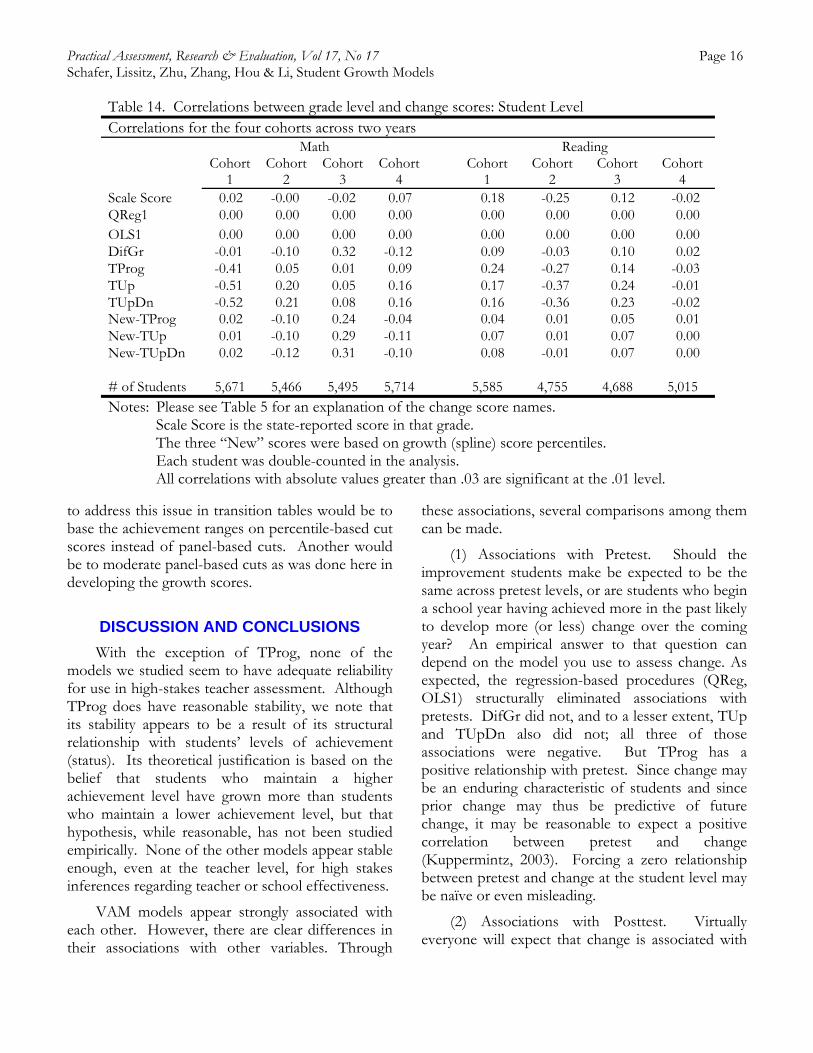
In order to study whether the six models are fair across grade levels, we correlated grade level with change score. Table 14 shows the student-level correlations between grade and change scores for all cohorts. For each cohort, there were two records per student, one change score for the earlier grade and one for the later grade, each paired with the grade from which the score derived. So the first

student in Cohort 1 was represented by one record with the grades 3-4 change score and a second with the grades 4-5 change score. The correlations tended to show significant correlations with grade level for the transition-table measures, which compromises comparisons among teachers in different grades. Associations for math were stronger than for reading in both analyses, suggesting that the achievement levels may be more differentiated across grade levels in math, and perhaps this is especially the case for math in the earlier grades in our data set.

In order to study the effects on change scores of grade-level differences in idealism (or realism) of the state’s achievement level cut scores, we created another set of cuts, dividing the growth (spline) score scale into nine equal-width categories and re-applied the three value tables. The results are in the last three rows of Table 14.

Except for Cohort 3 math (for which there may be an instructionally related explanation), associations with grade level decreased when applying growth-score-based cuts. One possible way

Table 13. Correlations with Other Variables for Math 2008 (Grade 3) to 2009 (Grade 4)

Change Measure

Existing Variable

Year 1 Year 2 Gender SpEd LEP FRM AfAm White

QReg1 0.00 0.50 0.01 0.00 0.01 -0.13 -0.11 0.09

OLS1 0.00 0.53 0.01 0.00 0.03 -0.14 -0.12 0.09

DifGr -0.34 0.13 0.00 0.07 0.05 0.00 0.00 0.00

TProg 0.52 0.82 0.01 -0.08 -0.04 -0.28 -0.25 0.20

TUp -0.28 0.12 -0.01 0.07 0.06 0.01 -0.01 0.00

TUpDn -0.26 0.17 0.00 0.05 0.05 -0.03 -0.02 0.02

n 5,689 5,689 5,689 5,287 5,553 5,689 5,689 5,689

Notes: Year1 and Year 2 are scale scores in grades 3 and 4, respectively. Gender was coded male = 0 and female = 1. SpEd was coded 1 if special education; 0 otherwise. LEP was coded 1 if limited English proficient; 0 otherwise. FRM was coded 1 if eligible for free or reduced-price meals; 0 otherwise. AfAm wac coded 1 if African American; 0 otherwise. White was coded 1 if white; 0 otherwise. Please see Table 5 for the explanations of the change measures. All correlations with absolute values greater than .03 are significant at the .01 level.


to address this issue in transition tables would be to base the achievement ranges on percentile-based cut scores instead of panel-based cuts. Another would be to moderate panel-based cuts as was done here in developing the growth scores.

DISCUSSION AND CONCLUSIONS

With the exception of TProg, none of the models we studied seem to have adequate reliability for use in high-stakes teacher assessment. Although TProg does have reasonable stability, we note that its stability appears to be a result of its structural relationship with students’ levels of achievement (status). Its theoretical justification is based on the belief that students who maintain a higher achievement level have grown more than students who maintain a lower achievement level, but that hypothesis, while reasonable, has not been studied empirically. None of the other models appear stable enough, even at the teacher level, for high stakes inferences regarding teacher or school effectiveness.

VAM models appear strongly associated with each other. However, there are clear differences in their associations with other variables. Through

these associations, several comparisons among them can be made.

(1) Associations with Pretest. Should the improvement students make be expected to be the same across pretest levels, or are students who begin a school year having achieved more in the past likely to develop more (or less) change over the coming year? An empirical answer to that question can depend on the model you use to assess change. As expected, the regression-based procedures (QReg, OLS1) structurally eliminated associations with pretests. DifGr did not, and to a lesser extent, TUp and TUpDn also did not; all three of those associations were negative. But TProg has a positive relationship with pretest. Since change may be an enduring characteristic of students and since prior change may thus be predictive of future change, it may be reasonable to expect a positive correlation between pretest and change (Kuppermintz, 2003). Forcing a zero relationship between pretest and change at the student level may be naïve or even misleading.

(2) Associations with Posttest. Virtually everyone will expect that change is associated with

Table 14. Correlations between grade level and change scores: Student Level Correlations for the four cohorts across two years Math Reading Cohort

1 Cohort

2 Cohort

3 Cohort

4 Cohort

1 Cohort

2 Cohort

3 Cohort

4 Scale Score 0.02 -0.00 -0.02 0.07 0.18 -0.25 0.12 -0.02 QReg1 0.00 0.00 0.00 0.00 0.00 0.00 0.00 0.00 OLS1 0.00 0.00 0.00 0.00 0.00 0.00 0.00 0.00 DifGr -0.01 -0.10 0.32 -0.12 0.09 -0.03 0.10 0.02 TProg -0.41 0.05 0.01 0.09 0.24 -0.27 0.14 -0.03 TUp -0.51 0.20 0.05 0.16 0.17 -0.37 0.24 -0.01 TUpDn -0.52 0.21 0.08 0.16 0.16 -0.36 0.23 -0.02 New-TProg 0.02 -0.10 0.24 -0.04 0.04 0.01 0.05 0.01 New-TUp 0.01 -0.10 0.29 -0.11 0.07 0.01 0.07 0.00 New-TUpDn 0.02 -0.12 0.31 -0.10 0.08 -0.01 0.07 0.00 # of Students 5,671 5,466 5,495 5,714 5,585 4,755 4,688 5,015 Notes: Please see Table 5 for an explanation of the change score names. Scale Score is the state-reported score in that grade. The three “New” scores were based on growth (spline) score percentiles. Each student was double-counted in the analysis. All correlations with absolute values greater than .03 are significant at the .01 level.


posttest. Other things the same, the higher you achieve, the more improvement you probably developed over the year. All the models were positively associated with posttest, but there were also striking differences. The weakest associations were for TUpDn, DifGr and TUp. The strongest association was for TProg. The associations for the regression-based procedures were in between.

(3) Associations with Demographics. One popular criticism of the use of posttests as school (or teacher) effectiveness measures is that characteristics of students that are beyond the control of institutions are highly correlated with posttests. Many, but not all expect that change measures will compensate for student demographics and provide an alternative that is more dependent on what actually happens during a year of schooling (Newton et al., 2010). In our data, correlations of all the procedures with gender, special education eligibility, and limited-English proficiency were all satisfyingly low. DifGr, TUpDn and TUp were all virtually uncorrelated with free or reduced-price meals eligibility. The parallel correlations for the regression-based procedures were low, but not as low, and the correlation for TProg was a bit higher, yet even for TProg, the predictability of change from meals status was under 8%. Correlations with African-American vs. other races showed the same pattern but were slightly weaker.

(4) Associations with Grade Level. Achievement levels are commonly set independently at each grade level and content combination. As a consequence, there are striking differences within almost every state in the degrees of idealism/realism expressed in their resulting cut scores across years and contents (Schafer, Liu, & Wang, 2007). A danger in using those cut scores to measure change, as do the transition procedures, is that they may be unfair to teachers in different grades (or contents). We studied that by correlating grade level with change score and found some relationships at some grades. In general, these decreased when we re-calculated the achievement levels using a method that was based on moderated cut scores. Therefore, we recommend that if transition tables are used, they should be based on moderated achievement

levels in order to remove or at least reduce bias due to grade level and content differences.

We did not have a vertical scale available in our data set. We tried to address the vertical scale concept (e.g., defining a change score by subtracting a pretest vertical scale score from a posttest vertical scale score) by using growth (spline) scores that were created independently based on a moderated norms table developed for each assessment using 2008 statewide data. We found this approach, and if the parallelism argument holds, a vertical-scale approach, to be disappointing. As can be expected from the regression-to-the-mean phenomenon, correlations with pretest were negative. We suspect the same outcome would result from a vertical scale, which could in addition suffer from artificial and invalid grade-to-grade variance.

We included ordinary least-squares regression in part to study the value of using quantile regression, as is popular in several states. We found little difference between the two. Based on our results, one seems about as good as the other in every way we evaluated them. We also found little advantage in including more than one year’s pretest in either approach.

Both regression-based approaches we studied involve re-estimation of the regression equations each year. When this is done, the outcomes become norm-based in such a way that the entire system cannot show trend in their change measures over extended time periods. Indeed, individual teachers might improve, but due to general improvement as well, that improvement might not be represented in the change scores of their students, since general improvement of the entire system cannot usually be studied.

Like DifGr, the transition-based procedures do not suffer from this structural drawback. It would be possible to use the regression-based procedures with equations that were generated from a base year and thus could show change over time. If that is not done, only norm-based inferences using the current year as the basis for the norms are possible.

As educators work to refine their understandings of changes in students, several directions for research seem promising.


1) Interactions could be modeled. Why should we insist on modeling teacher effects as though all students reacted the same way or even that all teachers are the same from day to day or over a year’s time, independent of the school and the nature of students? Although aptitude-treatment research has been disappointing at the student level, perhaps classrooms and school contexts can be shown to moderate teacher effects.

2) An increase in the exploration of school context effects and classroom context effects should be on our agenda. Our results are quite modest, but they indicate there does seem to be an effect worth studying. Right now, we do not think we can be confident that we know what that effect looks like. That will come from developing theory driven research. This effort can be used incorporated into the direction in point (1).

3) Our data seem to come from a district that is above average in its state and perhaps different in variability as well. The correlations may have been affected by the ranges of the variables in the data we had. There are, of course, at least three important sources of variability: students, teachers, and schools. Any of these may have been unusually homogeneous or heterogeneous, typical or atypical in our data. Replicating our work with other data sources should help evaluate whether our results are in line with the findings of others or are outliers. Other methodological dimensions for studying replication include our choices to delete data from small classrooms and from students who did not provide scores for all three years.

4) We cannot at this time encourage anyone to use VAM in a high stakes endeavor. If one has to use VAM, then we suggest a two-step process to initially use statistical models to identify outliers (e.g., low-performing teachers) and then to verify these results with additional data. Using independent information that can confirm or disconfirm is helpful in many contexts. The value of

this use of evaluative change results could be explored in further research efforts.

5) It makes a difference what VAM model we implement. Different teachers may be identified and their effectiveness may be estimated at different levels. Of course, we can use more than one model at a time. Also, we can and should choose our models based on policy decisions that capture the goals and intent of a school system. Multiple models can easily be generated from the data once they are assembled, as we did, and can be used to cover the policy goals of a broad range of stakeholders. The quality of the decisions reached using components of such a system as well as the full system itself could be a useful direction for inquiry.

6) Beginning to relate VAM to what teachers are actually doing is an important direction in which research could proceed. Creating causal models and exploring them with experiments could be a promising direction.

7) The lack of an agreed-upon outcome criterion for excellence in teaching could be addressed. If we had such a variable, we could compare VAM (and other) approaches on their associations with it. However, to expect the outcomes of schooling to be capable of representation in one or even only a few variables may not yield a fair representation of success. Perhaps several criteria are necessary, which could also be an interesting direction for further work.

8) Perhaps a better way to conceive educational program success is to characterize the challenges faced by educators and to compare programs based on success in meeting those specific needs (as suggested by Goe et al., 2008). For example, urban schools, rural schools, and suburban schools exist in distinctly different environments and expecting a variable such as a pretest score to represent a common construct among them seems unrealistic. Besides geography, variables such as socioeconomic status, individual aptitude, home environment, and per-pupil expenditure while associated with


each other, nevertheless may all be needed to represent institutional (school or individual teacher) challenge adequately. Constructing models to incorporate variables such as these and comparing outcomes with programs that have common environments may prove to have more value than VAM.

Policy-level interest in VAM has existed for over 25 years and is likely to intensify. We expect our understandings about how to assess change will expand significantly over the next 25 years. As we move forward, we hope our practice does not exceed our ability to support it technically.

References

Betebenner, D. W. (2008). Toward a normative understanding of student growth. In Ryan, K. E. and Shepard, L. A., editors, The Future of Test-Based Educational Accountability, 155–170. Taylor & Francis, New York.

Betebenner, D. W. (2012). Growth, standards, and accountability. In Cizek, G., editor, Setting Performance Standards: Foundations, Methods, and Innovations, 439–450. Routledge, New York.

Cohen, J. (1977). Statistical power analysis for the behavioral sciences (2nd ed.). New York: Academic Press.

Corcoran, S. P. (2010). Can teachers be evaluated by their students' test scores? Should they be? The use of value-added measures of teacher effectiveness in policy and practice. Annenberg Institute for School Reform, Providence, RI.

Danielson, C. (1996). Enhancing professional practice: A framework for teaching. Alexandria, VA: Association for Supervision and Curriculum Development.

Dawes, R. ( 1979) The robust beauty of improper linear models in decision making. American Psychologist, 34(7), 571-582

Goe, L., Bell, C., & Little, O. (2008) Approaches to Evaluating Teacher Effectiveness: A Research Synthesis. Washington, DC, National Comprehensive Center for Teacher Quality.

Glazerman, S, Loeb, S, Goldhaber, D., Staiger, D., Raudenbush, S., & Whitehurst, G. (2010). Evaluating Teachers: The important role of value-added. Brown Center on Education Policy at Brookings November 17, 2010.

Goldhaber, D., & Hansen, M. (2010). Assessing the Potential of Using Value-Added Estimates of Teacher Performance for Making Tenure Decisions. Working paper 31. Washington, D.C.: CALDER.

Hanushek, E. A. (1986). The Economics of Schooling: Production and Efficiency in Public Schools. Journal of Economic Literature.

Hill, H. C., Kapitula, L., & Umland. K. (2011). A validity argument approach to evaluating teacher value-added scores. American Educational Research Journal, 48(3), 794-831.

Hill, R., Gong, B., Marion, S., DePascal, C., Dunn, J., & Simpson, M. (2005). Using Value Tables to ExplicitlyValue Student Growth, Conference on Longitudinal Modeling of Student Achievement. Dover, NH: The Center for Assessment. Downloaded June 17, 2012 from http://www.nciea.org/publications/MARCES_RH07.pdf.

Koedel, Cory and Julian R. Betts. 2007. “Re- Examining the Role of Teacher Quality in the Educational Production Function.” Working Paper #2007-03. Nashville, TN: National Center on Performance Initiatives.

Kupermintz, H. (2003). Teacher effects and teacher effectiveness: A validity investigation of the Tennessee Value Added Assessment System. Educational Evaluation and Policy Analysis, 25(3), 287–298.

Lipscomb, S, Teh, B., Gill, B., Chiang, H., & Owens, A. (2010) Teacher and principal value-added research findings and implementation practices. Mathematica Policy Research, Inc.

Lissitz, R. W. (2012) The evaluation of teacher and school effectiveness using growth models and value added models: Hope versus reality. Vancouver, BC: AERA, Division H invited address.

Mandeville, G. K. (1988). School effectiveness indices revisited: Cross-year stability. Journal of Educational Measurement, 25(4), 349-356.

Mandeville, G. K., & Anderson, L. W. (1987). The stability of school effectiveness indices across grade levels and subject areas. Journal of Educational Measurement, 24(3), 203-216.

Maryland Assessment Research Center for Education Success (2012). A comparison of VAM models. Retrieved June 18, 2012 from http://marces.org/completed/FINALTechnicalReportVAM.doc.


McCaffrey, D. F., Sass, T. R., Lockwood, J. R., & Mihaly, K. (2009). The intertemporal variability of teacher effect estimates. Education Finance and Policy, 4(4), 572-606.

Newton, X. A., Darling-Hammond, L., Haertel, E., & Thomas, E. (2010). Value-added modeling of teacher effectiveness: An exploration of stability across models and contexts. Education Policy Analysis Archives, 18(23), 1-22.

Nitko, A. J. (2001). Educational assessment of students, (3rd ed.). Upper Saddle River, NJ: Merrill.

Papay, J.P. (2011) Different tests, different answers: The stability of teacher value added estimates across outcome measures. American Educational Research journal, 48,163-193.

Prince, C. D. Schuermann, P. J., Guthrie, J. W., Witham, P. J., Milanowski, A. T., & Thorn, C. A. (2009) The other 69 percent: Fairly rewarding the performance of teachers of non-tested subjects and grades. Center for Educator Compensation Reform http://www.cecr.ed.gov/guides/other69Percent.pdf (page 5).

Rockoff, J E. (2004) The impact of individual teachers on student achievement: Evidence from Panel Data. The American Economic Review, 94, 2, 247-252.

Rubin, D. B., Stuart, E. A., & Zanutto, E. L. (2004) A potential outcomes view of value-added assessment in education. Journal of Educational and Behavioral Statistics, 29, 103-116.

Sanders, W.J., Ashton, J.J., & Wright, S.P. (2005) Comparison of the effects of NBPTS-certified teachers with other teachers on the rate of student academic progress. Arlington, VA: National Board for Professional Teaching Standards. Available: http://www.nbpts.org/UserFiles/File/SAS_final_NBPTS_report_D_-_Sanders.pdf [accessed July, 2012].

Sanders, W. L., & Horn, S. P. (1994). The Tennessee Value-Added Assessment System (TVAAS): Mixed-model methodology in educational assessment. Journal of Personnel Evaluation in Education, 8, 299-311.

Sanders, W. L., & Horn, S. P. (1998). Research findings from the Tennessee Value-Added Assessment System (TVAAS) database: Implications for educational evaluation and research. Journal of Personnel Evaluation in Education, 12(3), 247-256.

Sanders, W. L., & Wright, S. P. (2008) A Response to Amrein-Beardsley (2008) “Methodological Concerns About the Education Value-Added Assessment System. A SAS White paper.

Sass, T. R. (2008) The stability of value-added measures of teacher quality and implications for teacher compensation policy. Calder, Brief 4, November.

Schafer, W. D. (2006). Growth scales as an alternative to vertical scales. Practical Assessment, Research, and Evaluation, 11(4). [Available online: http://pareonline.net/getvn.asp?v=11&n=4].

Schafer, W. D. (2007). Comments on setting performance standards for schools in accountability programs: Policy, technical, and operational issues. National Council on Measurement in Education Convention, Chicago.

Schafer, W. D. (2008). Setting state standards for school change: A commentary on Arkansas’s experience. National Council on Measurement in Education Convention, New York City.

Schafer, W. D. & Hou, X. (2011). Test Score Reporting Referenced to Doubly-Moderated Cut Scores Using Splines. Practical Assessment, Research & Evaluation, 16(13). Available online: http://pareonline.net/getvn.asp?v=16&n=13.

Schafer, W. D., Hou, X., & Lissitz, R. W. (2009). Consideration of test score reporting based on cut scores (Technical report). College Park, MD: MARCES.

Schafer, W. D., Liu, M. & Wang, J (2007). Content and grade trends in state assessments and NAEP. Practical Assessment Research & Evaluation, 12(9). Available online: http://pareonline.net/getvn.asp?v=12&n=9

Tekwe, C. D., Carter, R. L., Ma, C., Algina, J., Lucas, M. E., Roth, J., et al. (2004). An empirical comparison of statistical models for value-added assessment of school performance. Journal of Educational and Behavioral Statistics, 29(1), 11

United States Department of Education (2009). Race to the Top Program Executive Summary. Washington, DC.

Webster, W. J., & Mendro, R. L. (1994). Identifying and rewarding effective schools: The Dallas School Acountability Program. Paper presented at the Center for Research on Educational Accountability and Teacher Evaluation (CREATE), National Evaluation Institute, Gatlinburg, TN.

Webster, W. J., & Mendro, R. L., Bembry, K. L., & Orsak, T. H. (1995). Alternative methodologies for identifying effective schools. Paper presented at the Annual Meeting of the American Educational Research Association, San Francisco, CA.


Notes:

This research was conducted by the Maryland Assessment Research Center for Education Success with funding provided through the Maryland State Department of Education. The opinions are solely those of the authors.

The authors are indebted to the Baltimore County (MD) School District for sharing the data used in this report, and to Mark Moody whose assistance included initial data processing and teacher-student pairings.

Citation:

Schafer, William D.; Lissitz, Robert W.; Zhu, Xiaoshu; Zhang, Yuan; Hou, Xiaodong & Li, Ying (2012). Evaluating Teachers and Schools Using Student Growth Models. Practical Assessment, Research & Evaluation, 17(17). Available online: http://pareonline.net/getvn.asp?v=17&n=17

Corresponding Author:

William D. Schafer, Affiliated Professor (Emeritus) Department of Educational Measurement, Statistics, and Evaluation University of Maryland College Park College Park, MD 20742 e-mail: wschafer [at] umd.edu Homepage: http://www.education.umd.edu/EDMS/fac/Schafer/Bill.html

evaluating teachers and schools using student growth models · evaluating teachers and schools...

Documents