evaluating the augmentation of army resupply with additive
TRANSCRIPT

ABSTRACT
MOORE, TIMOTHY ANDREW. Evaluating the Augmentation of Army Resupply with Additive Manufacturing in a Deployed Environment. (Under the direction of Dr. Thom Hodgson.)
This thesis models the problem of keeping a M109A6 operational while in a deployed
environment, comparing traditional resupply methods to additive manufactured spare parts. The
additive technology is co-located with the howitzer unit, establishing a decentralized supply chain.
Specifically, what conditions make it advantageous to deploy additive manufacturing technology to
produce spare parts printed on demand? This model can assist decision makers determining when
to augment a unit’s typical safety stock with a 3D printing facility that can satisfy a howitzer unit’s
demand rate while deployed comparing cost and lead-time to make the best decision possible.
The model utilizes MATLAB to perform a simulation on the parts request process. In
particular, the model was constructed so that different parameters could be manipulated based off
of preference from the decision maker. For instance, the demand rate can easily be increased or
decreased to simulate different phases of an operation or different environments altogether. For
the purposes of this paper only parts comprised of metal were considered in the demand rate
because those parts directly impact the validity of utilizing a Direct Metal Laser Sintering (DMLS)
printer. Secondly, the model incorporates fixed and variable costs to demonstrate the fiscal
requirements to implement such a program. Again, the parameters within the cost model can easily
be adjusted to accurately reflect competitive pricing for the additive equipment and it can also be
adjusted based on the unit size that the additive equipment is required to support.
Once the tools were built, it painted a realistic scenario for what conditions needed to be
satisfied for additive capability to be useful in a deployed environment. This analysis enhances
decisions that directly impact the capabilities of Soldiers in the most dire of situations: combat. The
goal of this thesis is to highlight the areas that need to be focused on within additive manufacturing
to become a realistic option for the military to adopt its technology. Ultimately, additive
manufacturing will have an impact on spare parts fulfillment. As has been demonstrated in the
civilian sector, companies that begin to invest early in the technology have begun to reap the largest
benefits and the military should follow suit to remain on the cutting edge.

© Copyright 2018 by Timothy Andrew Moore
All Rights Reserved

Evaluating the Augmentation of Army Resupply with Additive Manufacturing in a Deployed Environment
by Timothy Andrew Moore
A thesis submitted to the Graduate Faculty of North Carolina State University
in partial fulfillment of the requirements for the Degree of
Master of Science
Operations Research
Raleigh, North Carolina
2018
APPROVED BY:
________________________________ ________________________________ Cecil Bozarth Russell King
________________________________ Thom Hodgson
Chair of Advisory Committee

ii
DEDICATION
This work is dedicated to my wife, Kathleen. She is an amazing mother to my two children, Steven
and Caroline, and easily the best example of a selfless person. Thanks for allowing me to pursue my
goals while helping to raise a family.

iii
BIOGRAPHY Tim Moore was born and raised in Roanoke, VA before attending college at the United States
Military Academy at West Point, where he received a B.S. in Economics in 2008. Upon
commissioning as a Field Artillery Second Lieutenant in the United States Army he served as a
Platoon Leader and Company Fire Support Officer while deploying in support of Operation Iraqi
Freedom. He would go on to serve as a Battalion Fire Direction and Battalion Fire Support Officer
while deploying in support of Operation Enduring Freedom in Afghanistan. He commanded in the 1st
Brigade 41st Field Artillery Regiment at Fort Stewart, GA and completed two training rotations to
Europe in conjunction with our NATO partners. In the summer of 2016 he began to study Operations
Research at North Carolina State University and upon completion he will be assigned to the
Mathematics Department at West Point.

iv
ACKNOWLEDGEMENTS I would first like to thank Dr. Hodgson for providing guidance throughout the entire process, keeping
me on track. Additionally, I would like to thank Dr. King and Dr. Bozarth for being mentors right from
the start. Lastly, I would be remiss if I did not mention the help I received from my office mate,
Brandon McConnell. He saved me countless hours by being a sounding board and helping determine
the best approach for many of my decisions in the model.

v
TABLE OF CONTENTS LIST OF TABLES ...................................................................................................................................... vii
LIST OF FIGURES ................................................................................................................................... viii
LIST OF EQUATIONS ...............................................................................................................................ix
Chapter 1. INTRODUCTION .............................................................................................................. 1
1.1 Additive Manufacturing .......................................................................................................... 1
1.2 Define the Problem ................................................................................................................ 1
1.3 Objectives ............................................................................................................................... 2
Chapter 2. LITERATURE REVIEW ...................................................................................................... 3
2.1 Current State of Additive Manufacturing ............................................................................... 3
2.2 Background ............................................................................................................................. 4
2.2.1 Ill-Structured Costs ......................................................................................................... 5
2.2.2 Supply Chain ................................................................................................................... 6
2.3 Advantages/Disadvantages .................................................................................................... 8
2.3.1 Pros ................................................................................................................................. 8
2.3.2 Cons .............................................................................................................................. 10
2.4 Centralized vs. Distributed ................................................................................................... 11
2.5 Direct Manufacturing ........................................................................................................... 12
2.6 Ideal Candidate to Adopt...................................................................................................... 13
Chapter 3. DESCRIPTION OF DATA ................................................................................................ 15
3.1 Data Used ............................................................................................................................. 15
3.1.1 Data Sources ................................................................................................................. 15
3.1.2 Data Organization ......................................................................................................... 15
3.1.3 Data Cleansing .............................................................................................................. 16
3.2 Converting to Model Input ................................................................................................... 16
3.2.1 Arrival Rate (λ(t)) .......................................................................................................... 16
3.2.2 Service Rate (μ) ............................................................................................................. 19
3.3 Additional Model Inputs / Cost ............................................................................................ 25
Chapter 4. METHODOLOGY ........................................................................................................... 29
4.1 Development of Simulation .................................................................................................. 29
4.1.1 Simulation Setup .......................................................................................................... 29
4.1.2 Simulation Assumptions ............................................................................................... 32
4.2 Actual Simulation.................................................................................................................. 32

vi
4.3 Simulation Outputs ............................................................................................................... 32
Chapter 5. ANALYSIS ...................................................................................................................... 34
5.1 Case Study Scenario.............................................................................................................. 34
5.1.1 Scenario 1 – Decrease Allowable Part Size ................................................................... 34
5.1.2 Scenario 2 – Increase Build Speed ................................................................................ 35
5.1.3 Scenario 3 – Adjusting Military Unit Size ...................................................................... 36
5.2 Factorial Design Simulation Results ..................................................................................... 36
5.3 Requirements for Implementation....................................................................................... 39
Chapter 6. CONCLUSION ................................................................................................................ 41
6.1 Recommendations ................................................................................................................ 41
6.2 Future Work ......................................................................................................................... 42
6.3 Summary ............................................................................................................................... 43
REFERENCES ......................................................................................................................................... 44
APPENDICES ......................................................................................................................................... 47
Appendix A. Data Sets .......................................................................................................................... 48
Model Input ...................................................................................................................................... 48
A.1 RAND Data .............................................................................................................................. 48
A.2 Build Time Data ...................................................................................................................... 50
Appendix B. MATLAB R2016b Simulation Script .................................................................................. 51
Appendix C. R Regression Script ........................................................................................................... 59
Appendix D. StatFit2 Distribution Fitting.............................................................................................. 60
D.1 3 Battalions Demand Rate (orders per day) ............................................................................... 61
D.2 Battalion Demand Rate (orders per day) ................................................................................... 65
D.3 Battery Demand Rate (orders per day) ...................................................................................... 69
D.4 Gun Demand Rate (orders per day) ........................................................................................... 73
Appendix E. Factorial Design and Results ............................................................................................. 77

vii
LIST OF TABLES Table 3-1. Build Time Data based on Volume ...................................................................................... 21 Table 5-1. Baseline Data drawn from original RAND demand data. .................................................... 34 Table 5-2. Simulation results decreasing the allowable part size. ....................................................... 35 Table 5-3. Simulation results holding demand and allowable part size constant. ............................... 36 Table 5-4. Simulation results decreasing the demand rate. ................................................................ 36 Table 5-5. Factors for Simulations ........................................................................................................ 37 Table 5-6. Factorial Design Points for Simulations ............................................................................... 37 Table 5-7. Factorial Design Simulation Results (Lead Time in days) .................................................... 38

viii
LIST OF FIGURES Figure 3-1. Organization of Requisition Data .................................................................................... 16 Figure 3-2. Number of Orders Per Day .............................................................................................. 17 Figure 3-3. Goodness of Fit ................................................................................................................ 18 Figure 3-4. Fitted Density................................................................................................................... 18 Figure 3-5. Fitted Distribution ........................................................................................................... 18 Figure 3-6. Autocorrelation of Orders Per Day .................................................................................. 19 Figure 3-7. AM Build Process ............................................................................................................. 20 Figure 3-8. Regression Data Using R Software .................................................................................. 22 Figure 3-9. Linear Regression of Build Times Based on Volume ........................................................ 23 Figure 3-10. Simulation Process .......................................................................................................... 25 Figure 3-11. Total Cost Breakdown ..................................................................................................... 28 Figure 4-1. Requisition Simulation Process ....................................................................................... 29 Figure 4-2. Number of Orders By Day ................................................................................................ 30

ix
LIST OF EQUATIONS Equation 1. Baumers Build Time Estimation Formula ........................................................................ 21 Equation 2. Simple Linear Regression Model ..................................................................................... 21 Equation 3. Design Costs .................................................................................................................... 25 Equation 4. Setup Costs ...................................................................................................................... 26 Equation 5. Material Costs ................................................................................................................. 26 Equation 6. Production Costs ............................................................................................................. 27 Equation 7. Post-Production Costs ..................................................................................................... 27 Equation 8. Total Cost Formula .......................................................................................................... 27 Equation 9. Beta Distribution (min, max, p, q) ................................................................................... 31 Equation 10. Regression Model with Adjustable Build Rate ................................................................ 35

1
Chapter 1. INTRODUCTION
1.1 Additive Manufacturing
Additive manufacturing (AM) came to light in the 1980’s but has recently garnered the attention of
industry and hobbyists alike as a potentially time and cost effective way to make products. The
accessibility of 3D printing continues to broaden and the technology itself continues to become
more proficient and less expensive. The Economist recently went so far as to tout AM as a “third
industrial revolution” that has the potential to change manufacturing on a global scale (Whadcock,
2012). People looking to experiment in their homes have certainly bought in, eager to exploit the
new technology. In Wohler’s Report 2016, desktop 3D printer unit sales (less than $5,000) grew at
an astounding 69.7% in 2015, selling 278,385 machines (Wohlers, 2016 ). As Malcolm Gladwell put
it, “there is a simple way to package information that, under the right circumstances, can make it
irresistible” and 3D printing has certainly intrigued many (Gladwell, 2000). A tipping point is fast
approaching where AM becomes widely used to augment product manufacturing.
AM application in a military context could be widely beneficial, allowing for a faster and potentially
cheaper resupply of requested spare parts by simplifying the supply chain and reducing inventory
costs. The military lends itself to the adoption of AM because it frequently operates in hazardous
locations that naturally isolates its Soldiers from logistical resupply. In this scenario, the military
stands to gain the most from AM technology and it therefore deserves to be analyzed as a practical
option to augment traditional resupply methods.
1.2 Define the Problem
Like all companies, the military wants to save money when possible without cutting corners.
However, this goal is coupled with the more serious desire to equip its employees, Soldiers, with the
necessary equipment to deploy and win our nation’s wars. Considering these two tenets, AM
technology becomes a very attractive option to augment the military’s current resupply chain. The
problem, plainly put, is how can the military get necessary spare parts to the Soldier faster? Lead
time on ordered replacement parts needs to be reduced so that Soldiers are able to accomplish
their mission. If AM can bridge this gap, then what conditions need to be present and/or change
altogether to be implemented as an impactful program?

2
1.3 Objectives
This thesis provides a synopsis of all current AM studies in the literature review, highlighting many
of the advantages this technology can provide. The thesis goes on to describe a process, simulation,
for evaluating the feasibility of augmenting an Army supply chain with AM technology. The demand
data for parts requested was taken from actual units in Iraq during the US’s initial invasion.
Specifically, a M109A6 Paladin’s parts are analyzed to reflect a realistic demand rate for just one end
item. In this case, the Paladin is a self-propelled howitzer and is the main weapon system for a
mechanized artillery unit. This data is manipulated through a series of assumptions and fed into a
computer simulation in order to analyze the results. Lastly, these results are incorporated in realistic
recommendations for how the Army can potentially improve its supply chain practices.
The buzz surrounding 3D printing is undeniable; the potential to disrupt current supply chains and
even the entire manufacturing industry is plastered on every headline in the news. This thesis looks
to serve as a framework for military decision makers, politicians, contractors and generals, to utilize
in determining an appropriate application of AM for military resupply. Directly, what conditions
need to be satisfied for AM to be viable in a deployed environment? Although much of the current
literature is based on civilian companies, adoption and implementation by the military would
consider many of the same guidelines.

3
Chapter 2. LITERATURE REVIEW
The current consensus is that there are enormous advantages to harnessing the capabilities of AM
and many scholars have written extensively on this topic. The literature review aims to provide a
cogent synopsis of all relevant work that has been done on the implications of additive
manufacturing in order to highlight the research gap between well-structured costs analysis and
those of the ill-structured variety. Well-structured costs consist of material, labor, and
manufacturing system costs (Young, 1991). Ill-structured costs stand as the areas which can benefit
the military the most: transportation and inventory costs.
2.1 Current State of Additive Manufacturing
AM at its simplest is the process of joining materials to make objects from 3D model data, usually
layer upon layer, as opposed to subtractive manufacturing methodologies. The oldest technology,
Stereolithography (SLA), uses a photosensitive resin and exposes it to a UV laser beam to create the
product. The most common form of 3D printing is Fused Deposition Modeling (FDM) where a
thermoplastic filament is heated and melted layer by layer in the X/Y direction and lowered in the Z
direction. An emerging technology is Electron Beam Melting (EBM) that allows highly durable metals
to be formed under an electron beam in a high vacuum that melts the metal powder. For this thesis,
Direct Metal Laser Sintering (DMLS) is considered as the main AM technology. DMLS uses lasers to
fuse powdered metals into functional prototypes and end-use parts. The key understanding is that
AM technology is constantly improving and evolving so it is reasonable to expect that higher quality
products will be created more quickly and less expensively in the future.
The above-mentioned techniques and others have been adopted by companies in many different
civilian sectors including medical fields, aerospace, clothing, jewelry, prototyping, and even food
products. The raw materials used to create these products are constantly evolving and include
different types of steel, titanium, cobalt, plastic, Kevlar, nylon, glass, and aluminum to name a few.
Given the excitement and potential practicality behind AM technology, many notable companies
have begun to invest in AM to maintain their edge on current trends. Among these are GE (jet
engines, medical devices, and home appliance parts), Lockheed Martin and Boeing (aerospace and
defense), Aurora Flight Sciences (unmanned aerial vehicles), Invisalign (dental devices), Google
(consumer electronics), and the Dutch company LUXeXcel (lenses for light-emitting diodes, or LEDs)
(D'Aveni, 2015).

4
The fascination is warranted because AM allows for the creation of completely redesigned products:
lighter weight with new strength properties, combination of multiple parts into one, or rapidly
decreasing the time required to make a prototype into a reality. In a recent example, Amaero and
Monash University were able to make multiple prototypes of a rocket engine, tweaking complex
geometrical details, and save months of design time (Haria, 2017). However, in most circumstances
the technology is not low-cost enough and cannot produce products quickly enough to immediately
replace traditional manufacturing (TM). Nearly all academic studies up to date agree that AM
technology will serve best as a complement to machining rather than an outright replacement for
the foreseeable future (Bogers, Hadar, & Billberg, 2015). Despite that, the desire for AM to become
the primary production method is heavily present in many sectors and the companies that begin to
explore the uses of AM now will benefit the most later, once AM technology catches up to the
demand levels that TM currently satisfies.
One important factor to note about the AM industry is that a lot of companies that produce the
technology also own the raw materials to be able to print with AM. This creates a partially skewed
market because the suppliers do not face as much competition as they would if it were a well-
established technology. In the future, it is expected that more companies will enter the AM
production field, thus driving prices down to a more a competitive rate.
There are still many obstacles that prevent companies from adopting and implementing AM in their
own production processes. The largest problem is that AM simply cannot keep pace with large
volumes of demand. Regardless of how inexpensive the technology becomes, build times will have
to decrease drastically in order to produce at a rate sufficient for products in high demand. Another
hindrance that often gets overlooked is having the correct personnel in place to ensure that AM is
run properly. Not just anyone can hit “print” and be done with the production process. Highly
specialized engineers are required to create Computer Assisted Drawings (CAD) that serve as
blueprints for products being created through AM. Another large obstacle is maintaining the
physical printers as well as the quality of the products that are being printed. Again, existing
personnel would have to be trained on the AM technology or replaced altogether.
2.2 Background
The rise of 3D printing and additive manufacturing will replace the competitive dynamics of
traditional economies-of-scale production with an economies-of-one production model, at least for

5
some industries and products (Petrick & Simpson, 2013). Areas that stand to gain the most from AM
include: 1) Mass customization, 2) Resource efficiency, 3) Decentralization of manufacturing, 4)
Complexity reduction, 5) Rationalization of inventory and logistics, 6) Product design and
prototyping, and 7) Legal and security concerns (Mohr & Khan, 2015). Each of these areas are
explained in depth with relevant literature that supports the advantages of implementing AM and
relevant case studies that highlight some of these areas are further explained.
2.2.1 Ill-Structured Costs
Much of the relevant AM research that has been conducted does not accurately explain the
potential benefit that AM can provide to ill-structured costs. Ill-structured costs are generally
comprised of supply chain aspects. Inventory is a primary example of an ill-structured cost that
provides tremendous upside for AM technology. The resources spent producing and storing these
products could have been used elsewhere if the need for inventory were reduced. Suppliers often
suffer from high inventory and distribution costs. Additive manufacturing provides the ability to
manufacture parts on demand. Traditional production technologies make it too costly and require
too much time to produce parts on demand. The result is a significant amount of inventory of
infrequently ordered parts. This inventory is tied up capital for products that are unused. They
occupy physical space, buildings, and land while requiring rent, utility costs, insurance, and taxes.
Meanwhile the products are deteriorating and becoming obsolete. Being able to produce these
parts on demand using additive manufacturing reduces the need for maintaining large inventory and
eliminates the associated costs (Gilbert & Thomas, 2014).
In an (s-1, s) inventory model for spare parts, Sirichakwal & Conner demonstrated that the concept
of virtual inventory, made possible by AM, has many appeals for spare parts inventory management
especially in systems where inventory obsolescence and stock-out risk are of high importance. They
also showed that a reduction in holding cost has more impact on reducing the stock-out probability
when the average demand rate for spare parts is low. Additionally, lead time reduction can actually
have a negative impact on the stock-out probability (Sirichakwal & Conner, 2016).
Transportation is another huge aspect of the supply chain that AM technology looks to alter
drastically in the future. Additive manufacturing allows for the production of multiple parts
simultaneously in the same build, making it possible to produce an entire product in one step.
Traditional manufacturing often includes production of parts at multiple locations, where an
inventory of each part might be stored. The parts are shipped to a facility where they are assembled

6
into a product. Additive manufacturing has the potential to replace some of these steps for some
products, as this process might allow for the production of the entire assembly in one build. This
would reduce the need to maintain large inventories for each part of one product, reduce the
transportation of parts produced at varying locations, and reduce the need for Just-In-Time (JIT)
delivery (Thomas, 2016). Another substantial transportation impact is the location of the production
facility which can be nearer to the user and is described in detail in its own section due to its
importance.
2.2.2 Supply Chain
The supply chain includes purchasing, operations, distribution, and integration. Purchasing involves
sourcing product suppliers. Operations involve demand planning, forecasting, and inventory.
Distribution involves the movement of products and integration involves creating an efficient supply
chain (Robinson, 2015). AM provides the potential for many advantages in the manufacturing supply
chain. A noticeable benefit is dematerializing the supply chain itself. If there are fewer steps along
the chain, then efficiency increases and the chance for delays and disruptions decreases. Other
advantages include true Just-In-Time manufacturing, reduced set up, changeover time, number of
assemblies, and the elimination of waste (material, time, costs, distribution) (Tuck, Hague, & Burns,
2007). AM also enables JIT manufacture at the shop floor instead of JIT delivery of supplies to the
shop floor. As a result, non-value added activities such as material movement and inventory holding
can be reduced to a minimum. The result is a lean supply chain with low cost. Additionally, AM can
improve the responsiveness of an agile supply chain. A build-to-order strategy can be implemented
to ensure that no stockout would occur. The overriding cost for AM production is not labor but the
machines and raw materials, which makes it economical to locate production facilities near the end
customers. Lastly, it is possible to customize products to meet individual customer needs. This will
facilitate the implementation of a build-to-order strategy and increase responsiveness to customer’s
demands (Huang, Liu, & Mokasdar, 2013).
All businesses aim to be efficient at every level and collectively the industry has adopted the 6 Sigma
approach towards a lean and agile supply chain. Thomas et al (2014) described seven categories for
a company to focus on in order to become lean:
1) Overproduction: occurs when more is produced than is currently required by customers

7
2) Transportation: transportation does not make any change to the product and is a source
of risk to the product
3) Rework/Defects: discarded defects result in wasted resources or extra costs correcting
the defect
4) Over-processing: occurs when more work is done than is necessary
5) Motion: unnecessary motion results in unnecessary expenditure of time and resources
6) Inventory: is similar to that of overproduction and results in the need for additional
handling, space, people, and paperwork to manage extra product
7) Waiting: when workers and equipment are waiting for material and parts, these
resources are being wasted
AM has the potential to improve efficiency for each of these tenets.
Manufacturing and delivering products to customers require the efforts of various companies that
form the manufacturing supply chain. These companies may include raw material suppliers,
component suppliers, original equipment manufacturers, wholesalers/distributors, logistics service
providers, and retailers. In a supply chain, materials flow forward from suppliers through various
stages toward customers, whereas information and funds flow backward. As described, AM has the
potential to reduce the number of stages in the traditional supply chain. Specifically, AM technology
offers two opportunities: (1) to redesign products with fewer components and (2) to manufacture
products near the customers (i.e., distributed manufacture). The net effect is reduction in the need
for warehousing, transportation, and packaging (Huang, Liu, & Mokasdar, 2013). These elements
combined illustrate the enormous impact AM technology can bring to the manufacturing supply
chain.
Hasan and Rennie (2009) noted that a fully functional AM supply chain was not yet available in 2009
in the spare parts industry. The authors proposed a business model to enable such a supply chain.
The model is based on an e-business platform that provides the following services (Hasan & Rennie,
2009):
1) Sourcing: give buyers easy access to a pool of suppliers.
2) Demand identification: assist suppliers to identify customers and their demand.

8
3) Content display: provide an e-catalogue to display the products and services provided by the suppliers.
4) Transaction: enable the exchange of procurement information between the buyers and suppliers.
5) Promotion: help suppliers advertise their products and services.
2.3 Advantages/Disadvantages
2.3.1 Pros
This section consolidates the benefits of AM for particular industries to utilize. AM technology is
constantly evolving and the upside is seemingly limitless (Steenhuis & Pretorius, 2017). AM opens
opportunities for manufacturing companies in three regards: 1) AM offers the option of generating
objects that would have been impossible to make with any other technology, 2) AM can be used as
an automation technology which substitutes for human labor, and 3) AM allows for cost-efficient
switching from traditional mass production to new areas of mass customization (Thiesse, Wirth, &
Kemper, 2015).
As a result of Niaki & Nonino (2017), we can affirm that AM brought not only a process innovation
but also product innovation. This revolutionary technology allows for the fabricating of creative
products and construction of highly complex parts; sharing design and collaboration with consumers
with a low cost of modifications; enabling the full customization of parts with more functionality and
aesthetic appeal, which is impossible for general production to fabricate with traditional techniques.
In addition to introducing new products, AM leads to new markets. Therefore, it is reasonable to
expect a growing demand for AM as some firms in the study have found, as well as an increasing
willingness of consumers to pay more for the higher value offered. This higher value is influenced by
customer service through time-to-market reduction and full customization, and provides the
possibility to charge higher prices, especially for parts made in metal. Consequently, it influences
revenue in a positive way and is an attractive investment (Niaki & Nonino, 2017).
Another advantage is a simplified supply chain to increase efficiency and responsiveness in demand
fulfillment. AM is conducive to innovative design and enables on-demand manufacturing. As a
result, the need for warehousing, transportation, and packaging can be reduced significantly. With
proper supply chain configuration, it is possible to improve cost efficiency while maintaining
customer responsiveness using AM. With the advent of personal AM machine, the dream may come

9
true where customers can obtain desirable products economically whenever they want and without
leaving their homes (Huang, Liu, & Mokasdar, 2013).
Many specific case studies conducted include multiple different types of industry and reflect the
effect of AM’s benefits in their results. Hearing aid companies in particular have been one of the
most prevalent adopters of AM. In a specific case study, a hearing aid company bought AM
technology and produced parts in house instead of by a third party. Although the company needed
highly paid engineers to build the designs, new benefits far outweighed this downside. In fact, the
company accomplished this by emailing scanned ear canals to a company in Germany that already
had CAD model engineers. Since the CAD designs were now being sent electronically the process
allowed for distributed manufacturing. This scenario reduced lead time by eliminating physical
deliveries (email request of scanned ears). Overall, both companies in this case study were able to
increase material utilization and improve efficiency (Oettmeier & Hofmann, 2016). In another
empirical case study on a lamp company, the results showed the supplementary capacity of the AM
process and how it improved the supply chain (SC) performance in terms of lead time and total cost.
That work identified the research gap between AM and SC and gave a comprehensive investigation
of different performance indicators such as order fulfill rate and waste rate (Chiu & Lin, 2015).
Another case study described many of the themes highlighted in this section. Specifically, General
Motors offers a program called Retail Inventory Management (RIM) that allows dealers to return
parts that do not sell in 15 months without any penalty. While the dealership avoids paying for the
part, they still have money tied up in labor costs to stock the part, rent utilities, taxes, insurance,
and the opportunity cost associated with carrying the part. It is easy to see that a dealership which
implemented AM of parts on demand could significantly reduce
1) the type and quantity of spare parts needing to be stocked
2) procurement costs for parts the dealer would typically order from the manufacturer or another location
3) shipping costs for parts ordered as well as obsolete parts returned
4) costs involved in recall programs for malfunctioning parts
In addition, the dealer would always be assured of having parts that utilized the most current part
design (Beyer, 2014). Another auto maker has been using 3D printers since 2014 to produce tooling
components for use on the assembly line. Not only have direct manufacturing costs decreased

10
drastically for selected parts but lead time has been significantly reduced as well. One example of a
component transformed by AM was a “liftgate badge tool” which is used to precisely place the car’s
logo. Lead time dropped 89%, with outsourcing taking an average of 35 days and 3D printing just 4
(Jackson, 2017).
Lastly, in England two different types of companies were analyzed: wallpaper and chemical filter
suppliers. The decoupling point was moved upstream to allow for high levels of customization which
greatly enhanced the perceived value by customers. Through the adoption of AM, additional
processes resulted in value stream (VS) creation, which co-existed with existing VSs to enhance and
strengthen manufacturing (without replacing traditional methods or VSs). This provided both
companies with the ability to grow their business and capabilities further to compete, positively
impacting on their region with spillover of skill, knowledge and economic benefit (Rylands, Bohme,
Gorkin, Fan, & Birtchnell, 2016). The case study resulted in the following hypotheses:
1) Incorporating AM into the manufacturing system results in growth across VSs due to close client engagement during the co-creation process.
2) AM is not replacing existing manufacturing/VS, rather it is complementing a company’s offerings.
3) Unless the VS changes, the business impact is limited (engineering solutions rather business solutions).
4) AM knowledge centers are critical supply chain nodes for a company pull driven implementation process.
2.3.2 Cons
Many barriers still exist to the adoption of AM and it is important not to discount these aspects and
get swept up in the potential benefits. The results suggest the AM machine acquisition price and
personnel intensiveness are major obstacles to a distributed deployment of this technology in spare
parts supply chains (Khajavi, Partanen, & Holmstrom, 2014).
Another study reveals a number of disadvantages and challenges ahead of this emerging
technology. In terms of operational costs, any additional sources of expenses, such as depreciation
of machines, maintenance cost and, more significantly, higher prices of the material and machines,
need further development to be efficient. In the perspective of processing, potential health hazards
caused by some raw materials, small production platforms and the need for post-processing are the
most challenging aspects. In addition, a limited range of available raw material and a shortage of

11
suppliers lead to a high negotiating power for AM material suppliers, in spite of efforts to develop
new viable materials (Hao, Zhang, & Mellor, 2014) (Niaki & Nonino, 2017).
2.4 Centralized vs. Distributed
As mentioned above, the largest potential for a disruptive change in supply chain management is
the location of production. Holmstrom et al. (2010) proposed two different approaches to integrate
AM technology in the spare parts supply chain. The first approach is to use centralized AM capacity
to replace inventory holding. AM machines are deployed in centralized distribution centers to
produce slow-moving spare parts on demand. Producing parts in a centralized location has the
advantage of aggregating demand from various regional service locations to ensure that the
investment in AM capacity is well utilized. The disadvantage is that the produced parts need to be
shipped to the service locations, which results in an increase of response time. A method to mitigate
this issue by locating production at third party logistics (3PL) sites. Hence, once a part is printed it
can be immediately shipped to its final destination (D'Aveni, 2015). However, for certain parts that
are needed in the first line maintenance, inventory still needs to be carried in the service locations.
The centralized approach is desirable when parts produced using AM are limited and the required
response time is not critical. The second approach, distributed AM at each service location, is
suitable when the demand of AM producible parts is sufficiently high to justify the capacity
investment. The advantage of the distribution of AM is the elimination of inventory holding and
transportation costs and a fast response time. In addition to these two approaches, Holmstrom et al.
(2010) also contemplates the feasibility of mobile AM but concedes that there are many challenges.
The authors further discusses the trade-off between batch production and on-demand production,
and the trade-off between specialized and general purpose AM. The key variables considered are
materials and production costs, distribution and inventory obsolescence costs, and life-cycle costs
for the user. They concluded that on-demand and centralized production of spare parts is most
likely to succeed (Holmstrom, Partanen, Tuomi, & Manfred, 2010).
In a case study conducted on aircraft spare parts, it is shown that the advantages of AM technology
can be introduced into different stages of the aircraft spare parts supply chain. Again, the
centralized AM supply chain is more suitable for parts with low average demand, relatively high
demand fluctuation, and longer manufacturing lead time. The distributed AM supply chain is
suitable for parts with high average demand. It is also suitable for parts with very stable demand,

12
because in this case the benefit of demand aggregation in a centralized distribution center is greatly
diminished. It can also be used for parts with very short manufacturing lead time, especially if their
demand is low and unpredictable; because such parts can be produced on-demand. It is clearly
demonstrated that AM has the potential to change the conventional supply chain configuration. In
this industry it is possible to achieve inventory reduction, thus cutting inventory holding costs across
the entire supply chain (Liu, Huang, Mokasdar, Zhou, & Hou, 2014).
The potential advantages of using AM machines for the distributed production of aircraft spare parts
can be summarized as follows: lower overall operation costs, lower down time, higher potential for
customer satisfaction, lower capacity utilization, higher flexibility, fewer supply chain disruptions,
reduced need for inventory management and logistics information systems, and potential for
sustainability improvements as AM machines become smaller and more energy efficient (Khajavi,
Partanen, & Holmstrom, 2014). However, the same study identifies notable gaps that prevented a
distributed approach. To combat this, it was suggested that higher automation, lower acquisition
price, and shorter production time of AM machines are the factors that the producers of these
machines should aim to develop to enable radical change in spare parts supply chain operations
(Khajavi, Partanen, & Holmstrom, 2014).
Decentralized distribution can remain challenging to fully realize. In another study a company is
unable to do decentralized production because they do not have a consistent customer base,
therefore cannot predict where they are going to sell their product. As a result, post-production
processes and costs are high so decentralization would only increase costs (Hao, Zhang, & Mellor,
2014).
2.5 Direct Manufacturing
Although the intent behind this paper is to utilize AM technology to satisfy realistic demand rates, a
brief description of direct manufacturing cost research is deserved. In one of the first cost studies,
Hopkinson and Dickens (2001) calculated the average cost per part based on three assumptions: 1)
the system produces a single type of part for one year, 2) it utilizes maximum volumes, and 3) the
machine operates for 90% of the time. The analysis included labor, material, and machine costs.
Other factors such as power consumption and space rental were considered but contributed less
than one percent of the costs; therefore, they were not included in the results (Hopkinson &
Dickens, 2001). The cost of additive manufactured was later refined by Ruffo et al. (2006) using an
activity based cost model, where each activity is associated with a particular cost. They produced

13
the same product that Hopkinson and Dickens produced using selective laser sintering (Ruffo, Tuck,
& Hague, 2006). The cost model constructed in a more recent paper for EBM and DMLS
demonstrates that machine productivity forms a main driver of per-unit manufacturing cost. It also
suggests that this contributes to a general cost barrier to technology diffusion of AM into
mainstream manufacturing (Baumers, Dickens, Tuck, & Hague, 2016). All these studies and others
have to led to the conclusion that there is a value to be placed on the speed, versatility, and
adaptability of AM as it allows for just-in-time manufacturing. Further, AM is favored in small
production lots in which the higher cost of AM specific raw materials is offset by a reduction in fixed
costs associated with conventional manufacturing (Frazier, 2014).
2.6 Ideal Candidate to Adopt
AM appeals to many different industries and in particular, ones that suffer from a natural divide
from their customers and suppliers. For instance, space is a readily cited example for obvious
reasons: distance to a supply depot! Other forms of isolation are encountered when the machine or
blueprints required to produce an old part do not exist anymore. Additionally, a customer may be
isolated due to a hazardous location, i.e. a war zone (Peres & Noyes, 2006).
Although AM technology has yet to be truly incorporated into the spare parts supply chain, it has
been successfully used to supply certain consumer goods. Reeves (2010) described four such
businesses that have adopted AM: (1) Fabjectory that enables players of Second Life to purchase
models of individualized avatar characters, (2) FigurePrints that allows players of World-of-Warcraft
to order 1/16th scale models of their online gaming characters, (3) Landprint that offers
personalized 3D model of any place on earth, and (4) Jujups that offers a range of personalized gifts
such as photo frames, badges, mugs, and even chocolate. All of these companies looked to capitalize
on aforementioned benefits. In particular, with this type of business model, retailers do not carry
any inventory. Goods are produced on-demand either in-house or through subcontract to a third-
party manufacturer and then shipped directly to the customers. There is no need for warehousing
and distribution, although the final products still need to be shipped to customers. Customers can
design their own personalized products or obtain files of standard products online through a
technology service provider. The products can then be built by the customers using their personal
3D printer. This disruptive technology has the potential to drastically change the landscape of the
conventional manufacturing supply chain (Reeves, Tuck, & Hague, 2010).

14
Ultimately, the ideal AM market looks like: small production output, high product complexity, high
demand for product customization to individuals, and spatially remote demand for products. In the
long run, the largest payoff is for a company that can produce small batches to a customer that
desires customization (Weller, Kleer, & Piller, 2015). All of these cited articles provide key concepts
to consider within the AM industry but given the short amount of time AM has been prevalent,
generally lack data to quantify these concepts. The military could capitalize on many of these touted
benefits by producing spare parts with AM in a deployed environment; none more important than
reducing lead time. Adopting a distributed manufacturing technique could alter how Soldiers get
spare parts while deployed.

15
Chapter 3. DESCRIPTION OF DATA
3.1 Data Used
3.1.1 Data Sources
All of the demand data used in this paper was provided by RAND Corporation (Peltz, Halliday,
Robbins, & Girardini, 2005). The provided data displayed all part requisitions for Operation Iraqi
Freedom (OIF) during a 162 day period that spanned the initial invasion in 2003. Each requisition
within the data set had specific information pertinent to the entire supply process and a sample of
the data is provided in Appendix A.1. The most important pieces of information for this thesis
included quantity, weight, volume, price, request date, and delivery date. An important distinction is
the requisition data does not reflect true demand because it is supply side data, not consumption
data. Considering this data comes from OIF, it is plausible that units ordered parts based off not only
actual needs but projected needs as well. Ultimately, the requisition data used in this thesis is more
conservative comprising of supply side data.
Another data source was build time data. This was collected from MakerBot™ Thingiverse, an online
design community for discovering, making and sharing 3D printable things. Specifically, 53 different
products were selected that directly reflected build time and volume, Appendix A.2. The metal parts
were all built using Direct Metal Laser Sintering (DMLS) and ranged from simple to complex designs.
The parts varied enough to accurately reflect eventual Paladin part CAD models given that current
blueprints do not exist for Paladin spare parts. However, the data range was limited to smaller parts,
not fully reflecting all sizes of Paladin parts.
3.1.2 Data Organization
The requisition data was organized by only focusing on specific Unit Identification Codes (UIC) to
determine what parts were ordered by heavy artillery battalions (BNs). To manage the scope of data
points, 4th Infantry Division (4ID) was selected so only artillery BNs in 4ID are reflected in the data. It
is important to note that there were 3 artillery battalions requesting parts in the data set. The goal
was to have a list of Paladin spare parts requested during this 162 day period but the given data set
did not provide what end item (piece of Army equipment) each National Item Identification Number
(NIIN) corresponded to. In order to solve this problem, a heavy artillery battalion’s monthly
Document Control Register (DCR) was utilized to generate NIIN’s of spare part requisitions

16
specifically for a Paladin. The 4ID OIF data was scrubbed based off of the DCR which resulted in a list
of Paladin parts that were requested during the first 162 days of OIF. Lastly, this list was filtered
once more to only reflect spare parts made primarily of metal so that the demand rate used in the
simulation model was solely for M109A6 Paladin spare parts made of metal during the first 162 days
of OIF, Figure 3-1.
Figure 3-1 Organization of Requisition Data
3.1.3 Data Cleansing
Preparing the data was fairly straightforward for this data set. The first step was to eliminate
erroneous orders. This was accomplished by filtering the orders and changing any order for a
quantity of 0 to a quantity of 1. The assumption was made that if a supply clerk submitted the order
then at least 1 part was required. This means part quantity is always greater than equal to 1, not to
be confused with orders by day. There were multiple days during the 162 day period that no orders
were submitted. The next step was to augment the request and delivery dates to reflect a more
intuitive time. The supplied dates were provided with a Julian prefix for 2003, ex. 3053 represented
February 22nd, 2003. So 3000 was subtracted from all dates for easier interpretation.
3.2 Converting to Model Input
3.2.1 Arrival Rate (λ(t))
The first step was to generate a random number of orders for each day. The assumption was made
that although orders may realistically arrive at any point during the day, they would be compiled in a
queue and processed at the start of the next day for simplicity. The number of orders were

17
analyzed using StatFit2 and the descriptive statistics are displayed in Figure 3-2. Again, 162 (data
points) days were used and the data reflects that a maximum of 98 orders in one day were made
and mode of 7 orders a day occurred most frequently.
Figure 3-2 Number of Orders Per Day
Next, it was determined that a Weibull distribution, with shape parameter α = 1.10484 and scale
parameter β = 11.9755, was the best fit for the continuous arrival rate of orders, Figure 3-3. The null
hypothesis in this case is that the Weibull distribution is the proper distribution for the Number of
Orders Per Day data. The large p-values indicate weak evidence against the null hypothesis, so we
fail to reject the null hypothesis.

18
Figure 3-3 Goodness of Fit
Furthermore, the fitted density and distribution reflect that Weibull is an acceptable distribution to
generate random variables, Figure 3-4 & Figure 3-5.
Figure 3-4 Fitted Density
Figure 3-5 Fitted Distribution
Each day is assumed to be independent of one another. This is important because the simulation
treats each day as independent of the past. Furthermore, Figure 3-6 defends this assumption with

19
the auto-correlation data because none of the data is highly correlated, meaning the previous day
does not have a significant impact on the amount of orders made the next day.
Figure 3-6 Autocorrelation of Orders Per Day
The arrival rate (λ(t)), number of orders per day, in this thesis varied based off the scenario the
simulation was performing. For instance, the demand rate changed when different unit sizes were
considered. Since the original data was reflective of 3 battalions making order requests, the demand
rate decreased as the unit sizes decreased. All of the subsequent distribution fittings can be seen in
Appendix D for reference. Additionally, all of the different scenarios are described and displayed in
Chapter 5.
3.2.2 Service Rate (μ)
The first factor that needs to be satisfied to determine viability of AM implementation is for the
production rate to meet the demand rate. This was accomplished by creating a simulation in
MATLAB that kept track of the total sojourn time for requisitioned parts and discussed in further
detail in Chapter 4. Figure 3-7 provides a depiction of all factors that were considered in the build
time model. It is important to understand the entire process to accurately reflect the amount of
time it takes to print a part.
3.3.2.1 Setup Procedures
Holistically, every product to be printed needs to begin with a CAD model, file preparation. From
there, an engineer would be responsible for setting up the chamber and otherwise preparing the
machine for operation. Lastly, the engineer would release the build and the printing would begin. All

20
of the steps occurring during the setup phase were accounted for with a Beta distribution which is
described later in this section. This was selected because realistic bounds on setup times exist for
every 3D build.
Figure 3-7 AM Build Process
3.3.2.2 Build Procedures
The actual build time estimation, given all necessary information about the CAD model, can be
calculated precisely. In fact, there are many published papers that fully and accurately provide
formulas to estimate build time for additive manufacturing. Equation 1 describes a globally accepted
algorithm for estimating build times (Baumers, et al., 2012)
1) Fixed time consumption per build operation, 𝑇𝑇𝐽𝐽𝐽𝐽𝐽𝐽
2) Total layer dependent time consumption, obtained by multiplying the fixed time
consumption per layer, 𝑇𝑇𝐿𝐿𝐿𝐿𝐿𝐿𝐿𝐿𝐿𝐿, by the total number of build layers 𝑙𝑙
3) The total build time needed for the deposition of part geometry approximated by the
voxels. The triple Σ operator in Figure 3 expresses the summation of the time needed to
process each voxel, 𝑇𝑇𝑉𝑉𝐽𝐽𝑉𝑉𝐿𝐿𝑉𝑉 𝑉𝑉𝐿𝐿𝑥𝑥, in a three-dimensional array representing the discretized
build configuration

21
𝑇𝑇𝐵𝐵𝐵𝐵𝐵𝐵𝑉𝑉𝐵𝐵 = 𝑇𝑇𝐽𝐽𝐽𝐽𝐽𝐽 + �𝑇𝑇𝐿𝐿𝐿𝐿𝐿𝐿𝐿𝐿𝐿𝐿 × 𝑙𝑙� + � � � 𝑇𝑇𝑉𝑉𝐽𝐽𝑉𝑉𝐿𝐿𝑉𝑉 𝑉𝑉𝐿𝐿𝑥𝑥
𝑉𝑉
𝑉𝑉=1
𝐿𝐿
𝐿𝐿=1
𝑥𝑥
𝑥𝑥=1
Equation 1. Baumers Build Time Estimation Formula
Baumers (2012) is referenced to acknowledge that there is a sophisticated approach to estimating
build times. It is understood on a more simplistic level that build time is a function of the deposition
speed and the length of the deposition in each layer. Additionally, the speed is certainly affected by
the quality of the printer and the complexity of the part. However, all of these variables could not be
captured for Paladin parts that do not currently have CAD models so the assumption was made that
build time could be calculated given part volume. The statistical significance of this assumption is
reinforced by the linear regression in Figure 3-9. The previously mentioned Thingiverse data
reflected actual build times with their corresponding volumes, Appendix A.1.
Table 3-1 below shows a sample of the parts selected for the regression.
Table 3-1 Build Time Data based on Volume
part v (in^3) Total Print Time (hrs) calibration_angle 0.17 0.33 clip_mk1 0.01 0.07 DCU224C-M4-adapter 0.37 0.37 Desk_Knob 0.22 0.28 drawer_bracket 1.07 1.1 egranaje_carro 3.83 2.02 embudo_con 3.17 4.53
The regression was based on the following model in Equation 2.
𝑦𝑦 = 𝛼𝛼 + 𝛽𝛽𝛽𝛽 + 𝜀𝜀
y = PartBuildTime
α = intercept
β = scalar
x = PartVolume
ε = error term Equation 2. Simple Linear Regression Model
The expected response, 𝑃𝑃𝑃𝑃𝑃𝑃𝑃𝑃𝑃𝑃𝑃𝑃𝑃𝑃𝑙𝑙𝑃𝑃𝑇𝑇𝑃𝑃𝑃𝑃𝑃𝑃, is found by adding the intercept term (α) which is an
unknown and non-random parameter, to another unknown and non-random parameter (β),

22
multiplied by the known covariate, 𝑃𝑃𝑃𝑃𝑃𝑃𝑃𝑃𝑃𝑃𝑃𝑃𝑙𝑙𝑃𝑃𝑃𝑃𝑃𝑃, plus an error term (ε). The error term is assumed
to be independently and identically distributed N(0,𝜎𝜎2). The regression fitted an α parameter of
0.93994 and β parameter of 0.29150 with an R2 value of 0.8334, seen in Figure 3-8. Figure 3-9
displays the 53 points of build time data regressed using R software. Time is displayed in hours and
volume is in cubic inches. The regression’s intercept was not forced to 0 so that the model could
more accurately predict small volume build times.
Figure 3-8 Regression Data Using R Software

23
Figure 3-9 Linear Regression of Build Times Based on Volume
The volume for each Paladin part was plugged into the regression described above to get the build
time for each part. Of note, print speed can be optimized in a chamber if small batches are created
and products are printed simultaneously in the horizontal direction. This of course requires available
space in the chamber and identical raw material between parts. This level of fidelity was not
possible for the build time model in this thesis so it was assumed that only one part would be built
at a time.
3.3.2.3 Post Build Procedures
Now that the build process is complete, the printed part needs to be removed from the chamber.
Routine cleaning inside of the chamber would be conducted by the engineer once the product has
been removed.
The next and most obvious question that needs to be answered is quality of the product. If the
quality and control engineer fails that part for any reason, then the entire build process will need to
be repeated. For the build time model, this increases the amount of time and subsequently will

24
increase the cost in the following cost model because additional material is used. In discussions with
the Center for Additive Manufacturing and Logistics (CAMAL) at NC State, the assumption was build
failure occurs at a 10% rate.
However, if the part passes inspection then post build procedures would commence. Although
technology is improving rapidly, nearly all metal parts would have to undergo some kind of post-
treatment to finalize the production process. An emerging technology to augment finishing of metal
parts is Additive systems Integrated with subtractive Methods (AIMS). This is exciting technology
because the subtractive techniques replicate traditional finishing techniques. This method would
require custom tooling and fixtures but could be operated by one engineer (Manogharan, Wysk,
Harrysson, & Aman, 2015). For this model, heat treatment and part washing were directly
considered.
Once the product was completely finished the typical Army resupply system would initiate with
parts tracking and shipping through logistical convoys. Similar to setup times, a Beta distribution was
used to account for post processing times, with a realistic upper and lower bound.
The assumption was made to not incorporate utilization rate, hence the AM technology is available
to operate 24 hours a day. Routine maintenance would need to take place during natural lags in part
requests.
In summary, the model design is an Mt/GI/1 queue. The arrival process is a Non-homogeneous
Poisson process that utilizes a time varying rate, λ(t), to assign arrivals based off the predetermined
Weibull distribution (within each replication). The service rate is a general distribution accounted for
with the previously mentioned regression. Lastly, 1 server (3D printer) processes 1 part at a time for
the baseline scenario. Figure 3-10 provides an overview of the simulation, illustrating arrivals and
how each part request was serviced.

25
Figure 3-10. Simulation Process
3.3 Additional Model Inputs / Cost
Another factor that is of particular interest to decision makers in the military is cost. The cost model
was developed based off of knowledge gained through extensive research and actual
implementation of 3D printing facilities in the civilian sector. Design, setup, material, production,
and post processing costs were considered in the cost model described below.
The first consideration is the actual design for AM produced parts, Equation 3. This model accounts
for the incurred cost and effort that is required to produce a CAD model for existing Paladin parts. In
order to run the simulation, it is assumed that every existing part has the potential to be produced
with AM. Realistically the CAD models would be outsourced through a third party contractor, not
created by internal Army assets. With that being said, the time and money the third party invested
in creating the CAD models would be reflected in the purchase price of the CAD model rights. In an
effort to account for the design cost, this model made the following assumptions: 10 hours of design
time by a design engineer that earns $120,000 per year would be required for each unique part. This
works out to approximately $75,000 for all parts. This cost would then be spread across the total
amount of parts to be produced. The total number of parts was taken from the initial demand data
and the design costs were divided by the number of parts. Intuitively, this cost decreases as the
number of unique parts decreases.
𝐷𝐷𝑃𝑃𝐷𝐷𝑃𝑃𝐷𝐷𝐷𝐷𝑇𝑇𝑃𝑃𝑃𝑃𝑃𝑃𝑙𝑙𝐷𝐷𝑃𝑃𝐷𝐷𝑃𝑃 = 𝐸𝐸𝐷𝐷𝐷𝐷𝑃𝑃𝐷𝐷𝑃𝑃𝑃𝑃𝑃𝑃𝐸𝐸𝑃𝑃𝑃𝑃𝑃𝑃𝑙𝑙𝑦𝑦𝐸𝐸𝑃𝑃𝑃𝑃𝑃𝑃 ∗ 𝐷𝐷𝑃𝑃𝐷𝐷𝑃𝑃𝐷𝐷𝐷𝐷𝑇𝑇𝑃𝑃𝑃𝑃𝑃𝑃
Equation 3. Design Costs

26
Once a CAD model has been created there are incurred setup costs prior to the actual build process,
Equation 4. Certain parts require specific orientation in the chamber and it is the responsibility of
the experienced engineer to setup the build area/platform. A deterministic setup time of 7.2
minutes was used for the cost analysis (not the build simulation) and it was estimated that a fully
burdened engineer would average 2,000 hours per year.
𝑆𝑆𝑃𝑃𝑃𝑃𝑃𝑃𝑆𝑆𝐷𝐷𝑃𝑃𝐷𝐷𝑃𝑃𝐷𝐷 = (𝑆𝑆𝑃𝑃𝑃𝑃𝑃𝑃𝑆𝑆𝑇𝑇𝑃𝑃𝑃𝑃𝑃𝑃 ∗ 𝑁𝑁𝑃𝑃𝑃𝑃𝑁𝑁𝑃𝑃𝑃𝑃𝑁𝑁𝑁𝑁𝑃𝑃𝑃𝑃𝑃𝑃𝑙𝑙𝑃𝑃𝐷𝐷) ∗ 𝐸𝐸𝐷𝐷𝐷𝐷𝑃𝑃𝐷𝐷𝑃𝑃𝑃𝑃𝑃𝑃𝐸𝐸𝑃𝑃𝑃𝑃𝑃𝑃𝑙𝑙𝑦𝑦𝐸𝐸𝑃𝑃𝑃𝑃𝑃𝑃
Equation 4. Setup Costs
The next cost area to consider is the actual production of the product, Equation 5. Raw material
costs vary greatly and most certainly the prices will continue to fluctuate as more suppliers enter
such a competitive market. This model assumed a fixed price of $240 per pound of raw material
based off current research (Wohlers, 2016 ). The total volume processed was pulled from the
simulation, converted from cubic inches to pounds, and multiplied to determine the total material
cost. One of the previously described benefits of AM was the ability to reuse scrap parts from the
build because the raw material was pure. The assumption was made that a 10% salvage value would
be applied to each build.
𝑀𝑀𝑃𝑃𝑃𝑃𝑃𝑃𝑃𝑃𝑃𝑃𝑃𝑃𝑙𝑙𝐷𝐷𝑃𝑃𝐷𝐷𝑃𝑃𝐷𝐷 = 𝐸𝐸𝑃𝑃𝑅𝑅𝑀𝑀𝑃𝑃𝑃𝑃𝑃𝑃𝑃𝑃𝑃𝑃𝑃𝑃𝑙𝑙𝐷𝐷𝑃𝑃𝐷𝐷𝑃𝑃 ∗ 𝑆𝑆𝑃𝑃𝑃𝑃𝑃𝑃𝐷𝐷𝑝𝑝𝑃𝑃𝑃𝑃𝐷𝐷ℎ𝑃𝑃 ∗ 𝑆𝑆𝑆𝑆𝑃𝑃𝑃𝑃𝑆𝑆𝐸𝐸𝑃𝑃𝑃𝑃𝑃𝑃
Equation 5. Material Costs
Another area of the build that cannot be overlooked is probability of a build failure. Ideally, if an
engineer is observing the production process then they might be able to identify a defect before the
build is complete. Hence, saving time and money. However, for this model all build failures were
identified after the build was complete at a certain probability, (1 – p). This build failure was
accounted for during the simulation, hence reflected in the total volume processed.
The next set of costs dealt with production, Equation 6. The machine run time is partly determined
by a fixed investment in the purchase of AM equipment and then associated maintenance costs for
the life of the printer. The purchase price for a high-end DMLS printer was $750,000 and annual
maintenance was 10% of the purchase price. It was assumed that the Army would be responsible for
maintenance costs. The asset utilization was 100% so the assumption was made that maintenance
would be completed during natural lulls in production. The actual print time was determined based
off the average aforementioned service rate. Lastly, a generic assumption of a 2 year life span for
each printer was made based on current literature reviews.

27
𝑃𝑃𝑃𝑃𝑃𝑃𝑃𝑃𝑃𝑃𝑆𝑆𝑃𝑃𝑃𝑃𝑃𝑃𝐷𝐷𝐷𝐷𝑃𝑃𝐷𝐷𝑃𝑃𝐷𝐷 = (𝐴𝐴𝐴𝐴𝑃𝑃𝑃𝑃𝑃𝑃𝐷𝐷𝑃𝑃𝑃𝑃𝑃𝑃𝑃𝑃𝑙𝑙𝑃𝑃𝑇𝑇𝑃𝑃𝑃𝑃𝑃𝑃 ∗ 𝑁𝑁𝑃𝑃𝑃𝑃𝑁𝑁𝑃𝑃𝑃𝑃𝑁𝑁𝑁𝑁𝑃𝑃𝑃𝑃𝑃𝑃𝑙𝑙𝑃𝑃𝐷𝐷) ∗ �𝑃𝑃𝑃𝑃𝑃𝑃𝑆𝑆ℎ𝑃𝑃𝐷𝐷𝑃𝑃𝑃𝑃𝑃𝑃𝑃𝑃𝑆𝑆𝑃𝑃 + 𝑀𝑀𝛽𝛽𝐷𝐷𝑃𝑃𝐷𝐷𝑃𝑃𝐷𝐷
𝐴𝐴𝐴𝐴𝑃𝑃𝑃𝑃𝑙𝑙𝑃𝑃𝑁𝑁𝑙𝑙𝑃𝑃𝑇𝑇𝑃𝑃𝑃𝑃𝑃𝑃𝑇𝑇𝑃𝑃𝑃𝑃𝑃𝑃𝑃𝑃𝐷𝐷𝑃𝑃�
Equation 6. Production Costs
Once the build is complete the engineer must inspect the part to ensure it passes necessary quality
and control checks. For metal parts in particular, post-processing is essential. Similar to the setup
and machine run time costs, post-processing would involve some of the engineer’s time. It is
assumed that there is no failure rate during the post-processing steps and the spare part has passed
all inspections for quality once complete.
𝑃𝑃𝑃𝑃𝐷𝐷𝑃𝑃𝐷𝐷𝑃𝑃𝐷𝐷𝑃𝑃𝐷𝐷 = (𝑃𝑃𝑃𝑃𝐷𝐷𝑃𝑃𝑇𝑇𝑃𝑃𝑃𝑃𝑃𝑃 ∗ 𝑁𝑁𝑃𝑃𝑃𝑃𝑁𝑁𝑃𝑃𝑃𝑃𝑁𝑁𝑁𝑁𝑃𝑃𝑃𝑃𝑃𝑃𝑙𝑙𝑃𝑃𝐷𝐷) ∗ 𝐸𝐸𝐷𝐷𝐷𝐷𝑃𝑃𝐷𝐷𝑃𝑃𝑃𝑃𝑃𝑃𝐸𝐸𝑃𝑃𝑃𝑃𝑃𝑃𝑙𝑙𝑦𝑦𝐸𝐸𝑃𝑃𝑃𝑃𝑃𝑃
Equation 7. Post-Production Costs
Although one of the recognizable benefits of AM is the ability to print on-demand or JIT, there are
still overhead costs associated with setting up an AM facility. While the inventory cost of spare parts
on warehouse shelves decrease, there are still incurred fixed costs such as operating (energy costs)
and consumable items. Although acknowledged, these costs were not directly incorporated into the
cost model because of minimal impact on total cost.
Equation 8 reflects the total cost formula used in each trial and provides a point of reference for the
decision maker when implementing AM technology.
𝑇𝑇𝑃𝑃𝑃𝑃𝑃𝑃𝑙𝑙𝐷𝐷𝑃𝑃𝐷𝐷𝑃𝑃 = 𝐷𝐷𝑃𝑃𝐷𝐷𝑃𝑃𝐷𝐷𝐷𝐷𝑇𝑇𝑃𝑃𝑃𝑃𝑃𝑃𝑙𝑙𝐷𝐷𝑃𝑃𝐷𝐷𝑃𝑃𝐷𝐷 + 𝑆𝑆𝑃𝑃𝑃𝑃𝑃𝑃𝑆𝑆𝐷𝐷𝑃𝑃𝐷𝐷𝑃𝑃𝐷𝐷 + 𝑀𝑀𝑃𝑃𝑃𝑃𝑃𝑃𝑃𝑃𝑃𝑃𝑃𝑃𝑙𝑙𝐷𝐷𝑃𝑃𝐷𝐷𝑃𝑃𝐷𝐷 + 𝑃𝑃𝑃𝑃𝑃𝑃𝑃𝑃𝑃𝑃𝑆𝑆𝑃𝑃𝑃𝑃𝑃𝑃𝐷𝐷𝐷𝐷𝑃𝑃𝐷𝐷𝑃𝑃𝐷𝐷
+ 𝑃𝑃𝑃𝑃𝐷𝐷𝑃𝑃𝐷𝐷𝑃𝑃𝐷𝐷𝑃𝑃𝐷𝐷
Equation 8. Total Cost Formula
Figure 3-11 illustrates the cost breakdown in detail. It is evident that material costs dominate the
total cost function, implying that if raw material prices decreased then the total cost would decrease
significantly.

28
Figure 3-11. Total Cost Breakdown

29
Chapter 4. METHODOLOGY
4.1 Development of Simulation
This section describes in detail each step and subsequent inputs for the simulation model used in
this thesis.
The simulation was designed in MATLAB and provides 2 key outputs: total sojourn time and total
cost. All code is provided in Appendix B and an overview is depicted in Figure 4-1 and described in
detail below.
Figure 4-1 Requisition Simulation Process
4.1.1 Simulation Setup
The orders arrival rate was described in detail in 3.2.1 and a sample Weibull distribution is displayed
below. The histogram reflects the distribution that was calculated in StatFit2. For this histogram
5,000 samples were generated with the maximum number of orders in one day being 74 and the
mode being 1 which is acceptable given the initial data.

30
Figure 4-2 Number of Orders By Day
The simulation uses multiple sorted probability mass functions (PMFs) to ensure that the number of
orders per day are comprised of a realistic type and quantity of each spare part.
The first PMF created reflected a sorted list of all unique parts based on the likelihood of being
selected. The RAND data set provided 1,736 different orders during the 162 day period. These 1,736
orders totaled 7,904 parts. Of those 7,904 parts there were only 120 unique types. Utilizing a for
loop, the simulation setup scans the entire list of orders, categorizes like parts, and outputs the
probability that each part will be randomly selected. For instance, the most frequently ordered part
was a SWITCH ASSEMBLY with 0.136 probability of being selected.
Now that the type of part could accurately be selected at random, the quantity would need to be
known for that part. Again, a for loop scanned the sorted part list described above and recorded
every time that part was ordered and the subsequent quantity of that part. The result was a matrix
of probabilities for quantity for each unique part type. For instance, there was a 0.6907 probability
of ordering 1 SWITCH ASSEMBLY when a SWITCH ASSEMBLY was randomly selected.

31
Now that the type and quantity of parts for each order were determined it is easy to match the
volume from the original RAND data set with the unique type of part. The total volume was critical
in calculating the build time and subsequent cost of production.
Every time the simulation needed to generate a build time, it would simply call the sorted and
stored PMFs that were separate from the actual simulation. This setup made the simulation run
faster because less data needed to be computed for every iteration. Specifically, function handles
that can be seen in Appendix B were created that pulled from the stored PMFs when a build time
was needed.
Another major consideration for setup was configuring all time, t, in hours. The previously
mentioned Weibull distribution would then provide a random number of orders each day at
subsequent 24 hour intervals. Hours were chosen because most build times could take less than a
day to complete. The number of trials, x, was determined during the setup, resulting in pre-
generated arrival times of orders for x trials.
Lastly, the pre and post processing requirements described in 3.2.2 were incorporated using a Beta
distribution. A Beta distribution was selected because an engineer’s pre and post processing times
could easily vary based on experience or repetition but would not vary outside of likely minimums
and maximums. This model assumed that the most likely setup time is 0.12 hours, with a min of 0.1
hours and max of 0.2 hours. Whereas the most likely post processing time is 0.3 hours, with a min of
0.2 hours and max of 1 hour. Equation 9 describes the Beta distributions used in the simulation.
𝑁𝑁(𝛽𝛽) = 1
𝑃𝑃(𝑆𝑆, 𝑞𝑞)(𝛽𝛽 − 𝑃𝑃𝑃𝑃𝐷𝐷)𝑝𝑝−1(𝑃𝑃𝑃𝑃𝛽𝛽 − 𝛽𝛽)𝑞𝑞−1
(𝑃𝑃𝑃𝑃𝛽𝛽 − 𝑃𝑃𝑃𝑃𝐷𝐷)𝑝𝑝+𝑞𝑞−1
min ⩽ x ⩽ max
min = minimum value of x
max = maximum value of x
p = lower shape parameter > 0
q = upper shape parameter > 0
B(p,q) Beta Function Equation 9. Beta Distribution (min, max, p, q)
32
4.1.2 Simulation Assumptions
The assumptions that had the largest effects on total sojourn time centered around build time
estimates. The first assumption did not consider batch service rates. The second assumed that the
Paladin parts would behave linearly based off the Thingiverse build time data. This is easily
justifiable for small Paladin parts, consisting of 40 cubic inches and less, but became more significant
when considering large part volumes. These volumes forced extrapolation, far beyond what the
provided Thingiverse data included. Additionally, the Paladin part volumes were “packaged”
volume, rather than actual part volume. Ideally, the dimensions of the parts and surface area would
be known so that a multiple linear regression could fully and more accurately calculate the build
times. All of these assumptions were conservative, serving as a worst case scenario for
implementation.
The probability of failure was selected to be 10% for the simulations. This is in line with current
technology but could potentially worsen given an unstable environment that a military 3D printing
facility might find itself in.
All of the distributions have been defended in previous sections. In general, Beta distributions were
used for the pre and post processing times while a Weibull distribution with varying parameters was
used for the arrival rate of orders per day.
4.2 Actual Simulation
The simulation that was built for this thesis was a single-server queuing system with discrete events.
All of the stochastic nature in the ordering process was captured prior to the actual simulation so
that the simulation itself could run faster and more efficiently.
Given the pre-generated set of arrival times for each replication, the simulation would cycle through
all arrival times until reaching a predetermined stop time. Again, the arrival times reflect the
number of orders per day. For every iteration, the time the order arrived in the system and departed
the system were recorded. The service rate (μ) was generated from the same function handle
described above that provided a random pre-processing, build, and post-processing times.
4.3 Simulation Outputs
As previously mentioned, the information most pertinent to military decision makers would be lead
time and cost. This simulation provided both total sojourn time and an estimated total cost. The

33
sojourn time reflects the amount of time the order spent in the system, i.e. how long it would take
an engineer to setup the build chamber, print the entities of the order, and inspect the parts for
future use. The cost is the summation of everything required to produce the parts. Total volume
processed was determined to be an important stat, indicating the general capability of the 3D
printing system. With this being said, total volume was also recorded as an output for comparisons
between scenarios.

34
Chapter 5. ANALYSIS
5.1 Case Study Scenario
The original RAND data was scrubbed, as previously mentioned, to reflect metal Paladin parts for 3
BN’s during a 162 day period. The requisition data was adjusted based off allowable part size,
replicating smaller sized 3D printer build chambers. Table 5-1 reflects a decreasing size (in3)
threshold for allowable part requests based on the actual OIF data. For example, Baseline All
considered every part request, regardless of size. Whereas, Base less than 250 only considered parts
less than 250 cubic inches. Regardless of the size, it reflects that the mean lead time was
approximately 39 days. When considering the entire 162 day invasion period, it appears that due to
exterior conditions (security, changing unit locations, etc.) only about 4 resupplies were afforded
because all of the part sizes were fulfilled in approximately 39 days. The total cost is the wholesale
cost of the part and excludes transportation and overhead costs. The total volume processed is
displayed because it provides a consistent and logical way to visualize the total orders processed. It
follows that the total volume processed would decrease in line with the allowable part sizes because
fewer parts that had smaller volumes were considered. All subsequent scenarios are compared to
this baseline data. Lastly, each scenario was replicated 100 times to achieve acceptable confidence
intervals.
Table 5-1. Baseline Data drawn from original RAND demand data.
Lead Time (days)
Total Cost ($)
Total Volume Processed
(in^3) Mean Baseline All 39.94 $691,096 3,566,792 Base < 250 38.94 $349,508 355,078 Base < 100 38.57 $186,284 304,389 Base < 57 39.00 $184,327 129,237 Base < 40 39.50 $22,343 33,323
5.1.1 Scenario 1 – Decrease Allowable Part Size
In Scenario 1, the allowable part size was incrementally decreased starting with all parts considered,
then less than 250 cubic inches and so on. The results overwhelmingly indicate that 1 AM printer
cannot satisfy the full demand rate for 3 BN’s requesting Paladin parts. However, when the
allowable part size is limited to less than 40 cubic inches, then 1 AM printer can actually decrease

35
the average lead time from 39.50 days to 10 days. The obvious tradeoff deduced from Table 5-2 is
the cost. The cost balloons by nearly 72 times the original cost. Again, the major advantage of AM
technology is distributed manufacturing, so incorporating transportation costs into the baseline
could narrow these margins.
In general, the simulation reflects a higher total volume processed than TM because of the build
failure rate. However, less than 100 actually showed a decrease from the base which is most likely
explained by the high probabilities of selecting smaller parts in this threshold, i.e. it was very rare to
select parts close to 100 cubic inches.
Table 5-2. Simulation results decreasing the allowable part size.
5.1.2 Scenario 2 – Increase Build Speed
This scenario attempts to illustrate how advances in AM technology could impact satisfying the
demand rate. In the base simulation only 1 AM printer is utilized. Alternatively, this scenario mimics
utilizing 10, 20, and 30 AM printers. In order to test other options that might provide a more realistic
solution, 10 DMLS printers were considered. They were incorporated by adjusting the build time
coefficient, decreasing it by a factor of 10. Equation 10 displays the build speed function used with
the adjustable build time factor, τ.
𝑦𝑦 =(𝛼𝛼 + 𝛽𝛽𝛽𝛽)
𝜏𝜏+ 𝜀𝜀
Equation 10. Regression Model with Adjustable Build Rate
This build speed adjustment assumes that orders would be evenly and simultaneously spread
among all 10 printers. While this may not be true in practice, the assumption was made to provide
context on how much faster AM build speeds need to be to satisfy a realistic demand rate. However,
10 printers only reduced mean sojourn time to 608 days. The results indicate that even if AM
technology were able to increase build speed, reducing build time, by 30 times that still would not
be enough to meaningfully impact the service rate. As displayed in Table 5-3 the lead time remains
at 186 days with an increase of 30. For clarification, demand rate and part size were kept constant.
(in^3) Mean HalfwidthAll Parts 6,939 177.83 17272.83% $122,056,634 17561.31% 4,428,379 24.16%< 250 662 19.46 1600.48% $12,524,344 3483.42% 454,289 27.94%< 100 374 11.87 869.67% $7,028,465 3672.98% 254,886 -16.26%< 57 219 7.93 461.54% $5,093,894 2663.51% 184,695 42.91%< 40 10 0.66 -74.79% $1,630,834 7199.08% 59,047 77.20%
Difference From BaseLead Time (days)
Difference From Base Total Cost ($) Difference From BaseTotal Volume
Processed (in^3)
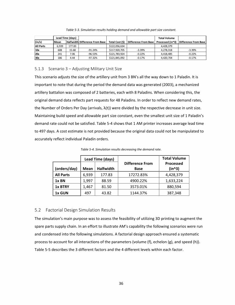
36
Table 5-3. Simulation results holding demand and allowable part size constant.
5.1.3 Scenario 3 – Adjusting Military Unit Size
This scenario adjusts the size of the artillery unit from 3 BN’s all the way down to 1 Paladin. It is
important to note that during the period the demand data was generated (2003), a mechanized
artillery battalion was composed of 2 batteries, each with 8 Paladins. When considering this, the
original demand data reflects part requests for 48 Paladins. In order to reflect new demand rates,
the Number of Orders Per Day (arrivals, λ(t)) were divided by the respective decrease in unit size.
Maintaining build speed and allowable part size constant, even the smallest unit size of 1 Paladin’s
demand rate could not be satisfied. Table 5-4 shows that 1 AM printer increases average lead time
to 497 days. A cost estimate is not provided because the original data could not be manipulated to
accurately reflect individual Paladin orders.
Table 5-4. Simulation results decreasing the demand rate.
Lead Time (days) Difference From
Base
Total Volume Processed
(in^3) (orders/day) Mean Halfwidth All Parts 6,939 177.83 17272.83% 4,428,379 1x BN 1,997 88.59 4900.22% 1,633,224 1x BTRY 1,467 81.50 3573.01% 880,594 1x GUN 497 43.82 1144.37% 387,348
5.2 Factorial Design Simulation Results
The simulation’s main purpose was to assess the feasibility of utilizing 3D printing to augment the
spare parts supply chain. In an effort to illustrate AM’s capability the following scenarios were run
and condensed into the following simulations. A factorial design approach ensured a systematic
process to account for all interactions of the parameters (volume (f), echelon (g), and speed (h)).
Table 5-5 describes the 3 different factors and the 4 different levels within each factor.
(in/s) Mean HalfwidthAll Parts 6,939 177.83 $122,056,634 4,428,37910x 608 15.68 -91.24% $117,920,705 -3.39% 4,278,318 -3.39%20x 241 7.06 -96.53% $121,783,924 -0.22% 4,418,485 -0.22%30x 186 4.44 -97.32% $121,845,092 -0.17% 4,420,704 -0.17%
Lead Time (days)Difference From Base Total Cost ($) Difference From Base
Total Volume Processed (in^3) Difference From Base
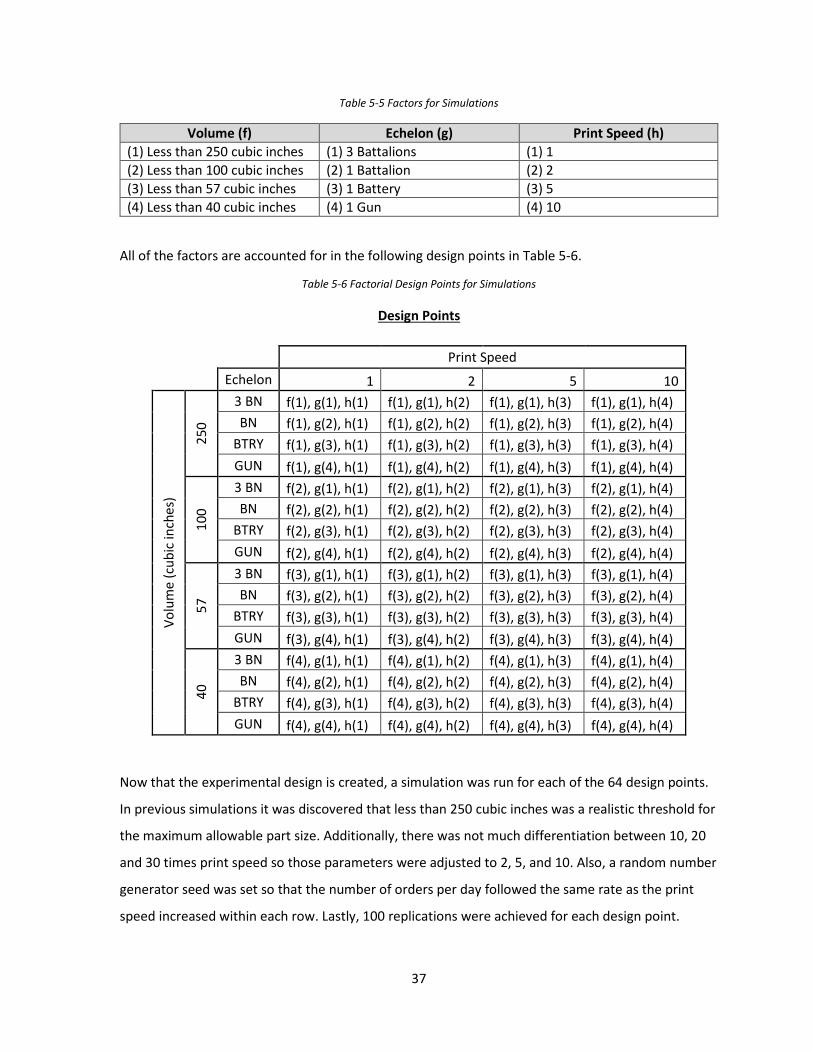
37
Table 5-5 Factors for Simulations
Volume (f) Echelon (g) Print Speed (h) (1) Less than 250 cubic inches (1) 3 Battalions (1) 1 (2) Less than 100 cubic inches (2) 1 Battalion (2) 2 (3) Less than 57 cubic inches (3) 1 Battery (3) 5 (4) Less than 40 cubic inches (4) 1 Gun (4) 10
All of the factors are accounted for in the following design points in Table 5-6.
Table 5-6 Factorial Design Points for Simulations
Design Points
Print Speed
Echelon 1 2 5 10
Volu
me
(cub
ic in
ches
)
250
3 BN f(1), g(1), h(1) f(1), g(1), h(2) f(1), g(1), h(3) f(1), g(1), h(4) BN f(1), g(2), h(1) f(1), g(2), h(2) f(1), g(2), h(3) f(1), g(2), h(4)
BTRY f(1), g(3), h(1) f(1), g(3), h(2) f(1), g(3), h(3) f(1), g(3), h(4) GUN f(1), g(4), h(1) f(1), g(4), h(2) f(1), g(4), h(3) f(1), g(4), h(4)
100
3 BN f(2), g(1), h(1) f(2), g(1), h(2) f(2), g(1), h(3) f(2), g(1), h(4) BN f(2), g(2), h(1) f(2), g(2), h(2) f(2), g(2), h(3) f(2), g(2), h(4)
BTRY f(2), g(3), h(1) f(2), g(3), h(2) f(2), g(3), h(3) f(2), g(3), h(4) GUN f(2), g(4), h(1) f(2), g(4), h(2) f(2), g(4), h(3) f(2), g(4), h(4)
57
3 BN f(3), g(1), h(1) f(3), g(1), h(2) f(3), g(1), h(3) f(3), g(1), h(4) BN f(3), g(2), h(1) f(3), g(2), h(2) f(3), g(2), h(3) f(3), g(2), h(4)
BTRY f(3), g(3), h(1) f(3), g(3), h(2) f(3), g(3), h(3) f(3), g(3), h(4) GUN f(3), g(4), h(1) f(3), g(4), h(2) f(3), g(4), h(3) f(3), g(4), h(4)
40
3 BN f(4), g(1), h(1) f(4), g(1), h(2) f(4), g(1), h(3) f(4), g(1), h(4) BN f(4), g(2), h(1) f(4), g(2), h(2) f(4), g(2), h(3) f(4), g(2), h(4)
BTRY f(4), g(3), h(1) f(4), g(3), h(2) f(4), g(3), h(3) f(4), g(3), h(4) GUN f(4), g(4), h(1) f(4), g(4), h(2) f(4), g(4), h(3) f(4), g(4), h(4)
Now that the experimental design is created, a simulation was run for each of the 64 design points.
In previous simulations it was discovered that less than 250 cubic inches was a realistic threshold for
the maximum allowable part size. Additionally, there was not much differentiation between 10, 20
and 30 times print speed so those parameters were adjusted to 2, 5, and 10. Also, a random number
generator seed was set so that the number of orders per day followed the same rate as the print
speed increased within each row. Lastly, 100 replications were achieved for each design point.

38
Table 5-7 Factorial Design Simulation Results (Lead Time in days)
Lead Time (days)
Print Speed
Echelon 1 2 5 10 Vo
lum
e (c
ubic
inch
es)
250
3 BN 782.84 362.08 109.85 25.83 BN 247.15 89.65 4.57 0.8
BTRY 109.79 17.68 1.13 0.56 GUN 9.81 2.26 0.96 0.42
100
3 BN 389.8 164.21 28.86 1.42 BN 105.19 16.61 0.84 0.4
BTRY 22.69 0.83 0.29 0.17 GUN 5.48 2.24 0.68 0.27
57
3 BN 278.39 107.55 5.94 0.9 BN 44.82 2.26 0.81 0.37
BTRY 4.54 3.21 0.67 0.33 GUN 2.82 1.61 0.52 0.29
40
3 BN 26.05 1.3 0.43 0.3 BN 1.65 2.32 0.74 0.35
BTRY 8.08 0.72 0.52 0.14 GUN 1.44 2.09 0.26 0.14
Using the results from Table 5-7, decision makers could implement AM technology at different
echelons (BN, BTRY, GUN) with a realistic understanding of the demand rate the 3D printer could
satisfy. For instance, all of the green shaded boxes indicate a lead time that was less than the
baseline of 39 days lead time determined from the OIF data. Table 5-7 displays a lot of scenarios
where AM produced parts could prove to be beneficial. Additional details are provided in Appendix
E which include half-width, cost, and total volume processed for each design point.
There are a few design points that do not appear to be monotonic. For instance, a battery’s demand
rate for parts less than 40 cubic inches at print speed 1 (f4, g3, h1) resulted in an increased lead time
when compared to a battalion’s. This was only true in the simulation because of the high probability
of selecting parts that were close to 40 cubic inches. A separate simulation was run that removed
the seed and increased the replications to 50,000. A more intuitive lead time of 1.94 days was
calculated. The takeaway is that less than 40 cubic inches was more sensitive to what parts were
selected from its PMF.

39
5.3 Requirements for Implementation
The likely scenario that AM will be most useful to the military is in an isolated deployed environment
where resupply is incredibly dangerous, expensive, or virtually impossible. In this scenario, the
ability to produce essential spare parts is invaluable.
There are many necessary requirements before 3D printing can even enter the conversation of
becoming a viable option for implementation. The simplest: can the spare part be printed with AM
technology? For this thesis to be at all relevant, it is assumed that all the spare parts can be printed
with on-hand technology at the established AM facility. Inherent in the ability to print is the
existence of CAD blueprints for the part. Naturally, all of these would theoretically exist in some
database that could be electronically transferred to the engineers that would be producing the parts
at a distributed location. In this model, the design cost is considered but it never terminates the
possibility of being able to physically print the spare part.
The AM equipment would need to be capable of global transport, most likely being outfitted in a
shipping container. Given the highly sensitive nature of metal 3D printers, studies would need to
ensure that the printing equipment would not be damaged in transit and could be setup, fully
functional, upon arrival to its destination.
From a strategic military standpoint, the capability needs to exist to build a facility. Security would
be the first and most paramount concern. Building an AM facility, whether it is a hardstand building,
a clamshell tent structure, or a CONEX container, implies that it can safely exist long enough to
effectively produce parts. Understanding if this facility could be secured with the unit’s internal
assets or would require additional attachments would be determined through practice on a mission
by mission basis.
Once security is established, more robust security element for a static location, consistent power
with enough wattage to run the AM systems would have to be setup. This would require a
redundant network of generators in most situations, perhaps tapping into a power grid in less
austere locations. For reference, DMLS printers can require up to 200 megajoule (MJ) per part or 55
kilowatt hour (kWh) (Baumers, Tuck, Wildman, Ashcroft, & Hague, 2011). The Army could furnish
enough power to run the printer but this obviously means that more equipment would have to be
deployed with that unit (i.e. generators). Furthermore, considering Scenario 2 where the build speed
is increased, the power requirements might be even greater. Unequivocally, if the AM facility had

40
more than just 1 printer then there would need to be additional power beyond just the standard
generators.
Another requirement is for the actual air in the facility to be regulated to avoid material
contamination during the build process. Most likely, an exhaust system would be necessary to
achieve a minimal standard for printing metal products. This would include maintaining a certain
humidity level, temperature, and dust free environment. Additionally, to meet the high tolerance
standards required in 3D printing, gases would need to be furnished. In most cases, Argon and
Nitrogen at a minimum are necessary to provide inert atmospheres for the printing process.
Mentioned throughout this thesis is the requirement for knowledgeable personnel to run the AM
equipment. Given the assumption that the 3D printer is most beneficial in an isolated environment
implies that the people utilizing the printer need to be highly competent on its capabilities,
limitations, maintenance: everything involved. Perhaps in the future when 3D printers are highly
reliable the Army could train Soldiers to use the printers but for now, contracted engineers are
required. Just as with power requirements, the more printers the more engineers are needed.

41
Chapter 6. CONCLUSION
There is no denying the potential disruptiveness that AM can have on industries by replacing or at
least complementing existing manufacturing techniques, specifically enhancing process and product
innovation (Niaki & Nonino, 2017). The military is currently looking at options to exploit this
technology and with an increased budget, decisions seem to be moving in the right direction. The
Navy has implemented FabLabs that consist of a suite of digital fabrication and rapid prototyping
machines. These mobile labs educate Soldiers on the capabilities of 3D printing and are an integral
step in making 3D printed parts a reality. As for now, the Marines cite examples of printing HUMVEE
handles and drone rotors to serve as temporary replacements while waiting for actual parts that
have been ordered to be received (Jackson, 2017).
In this thesis, a Paladin was used to demonstrate that a demand rate for a large piece of equipment
could be satisfied under certain constraints with current AM technology. However, there are
millions of parts in the military, many of which do not need to be as heavily scrutinized in a quality
control setting. Table 5-2 demonstrated that roughly 60,000 cubic inches is the threshold for total
output during a 162 day period. Along this line of thinking, any other end item could be selected and
roughly 60,000 cubic inches worth of spare parts could be printed for that item. One example of
other applications is with communications equipment. There are hundreds of small metal parts for
radios and antennas that constantly break through routine use by Soldiers. A 3D printer could make
communications spare parts while deployed and if the part failed during use, the only liability would
be a down radio. Whereas, if 3D printed parts were being used to fire a Paladin or a fly a helicopter,
the risk of injury from defective parts would be much higher.
6.1 Recommendations
The notion of 3D printed parts needs to start with CAD files. AM technology will never be fully
realized in a military setting if Soldiers are expected to create the part designs. Pressure needs to be
placed on contracted suppliers to either create CADs for existing parts or at a minimum, start
providing them with newly purchased equipment. This pressure would be applied many echelons
above the Soldier level. A steadily improving technology consists of sophisticated scanners that can
instantly produce a CAD blueprint. Perhaps this could stand as a viable option to bridge the gap
between TM and AM produced parts.

42
Similar to the Navy, the Army needs to continue experimenting with AM facilities in the field which
replicate realistic demand rates and environment scenarios. The most obvious choice is to utilize
existing environments at Combined Training Centers (CTC) and see how an AM facility performs. A
pilot program could consist of a 3D printing facility in a hardstand building at a CTC that receives
part requests from actual units training and then determines how many and what type of parts it
can print. This would start to give a feel for utilization rates, maintenance issues, troubleshooting
techniques, as well as provide an architecture to route the part requests from Soldier to 3D printing
engineer.
Real world applications would most likely start with smaller, more specialized units that deploy to
every corner of the globe and are not afforded consistent resupply. These types of units, suffering
from extreme isolation, could benefit the most from the implementation of a 3D printer.
Another application for AM technology would be in the sale of equipment to other countries. 3D
printed parts could substantially assist in providing spare parts to countries that have purchased
antiquated US military equipment. This is a large fiscal requirement because under most
circumstances, when the buyer requires additional spare parts they request them through the US.
The resupply then is even more costly because of additional overheard and transportation costs.
Imagine if, along with the initial purchase of the end item, CAD files were provided for all
components. Then the third party could furnish all future parts internally, eliminating time and
money spent by the US.
6.2 Future Work
Future work would need to focus on the direct comparison between traditional Army resupply and a
proposed pilot program utilizing additive manufacturing. Although it is easy to assume that
transportation and inventory costs would be dramatically decreased using AM, quantitative data
would help bolster this claim.
The demand rate changes drastically based off the phase of the operation. The demand rate in this
thesis is for an invasion but testing out different demand rates would give a better sense of how AM
could impact the supply chain over the course of a conflict. Additionally, only one end item, a
Paladin, was considered in this thesis. Testing the simulation on other end items would solidify if the
notion that “Total Volume Processed” is a good indicator of service capability.

43
Lastly, one of the largest ways to decrease build time is by batching part builds. This thesis lacked
enough fidelity on part descriptions to implement batching criteria. However, this could hold the
ability to dramatically decrease build times, thus increasing supply chain efficiency. Another
improvement when considering batching is to provide prioritization in the queue. This model used
first come first served (FCFS) basis but under the context of printing mission critical parts, reordering
the queue would be paramount. Perhaps the greatest use of AM technology would be to print parts
when TM lead time exceeds a certain threshold, subsequently providing the part to the Soldier
faster and getting their equipment back in the fight.
6.3 Summary
The simulation in this thesis provides a cogent process to evaluate the effectiveness when
integrating additive manufacturing technology in order to complement existing traditional
manufacturing techniques. It was determined, under current technology, that 1 DMLS printer could
satisfy the demand rate for a battalion’s M109A6 Paladin parts in a combat environment up to 57
cubic inches in total part volume. In order for AM to have a more drastic and ubiquitous impact,
faster build speeds for larger parts is the single point of improvement. Build rate failure is an
additional point of focus that will not only enhance lead time reduction but more importantly,
guarantee printed parts satisfy structural requirements creating minimal risk when used. Cost
reductions of raw materials and purchase price of printers will naturally occur as more competitors
enter the space and more efficient techniques are discovered for building printers.
AM will have an impact on the resupply of spare parts in the military, it is just a matter of when. The
Army Chief of Staff Gen. Milley understands this urgency and was recently quoted that “static bases
will be sitting ducks, and supply convoys will be so dangerous that they might be entirely
automated, so units will be largely on their own, purifying their own water and 3-D printing spare
parts for broken gear” (Freedberg, 2016).

44
REFERENCES Baumers, M., Dickens, P., Tuck, C., & Hague, R. (2016). The Cost of Additive Manufacturing: Machine
Productivity, Economies of Scale and Technology-push. Technological Forecasting and Social Change, 102, 193-201. doi:10.1016/j.techfore.2015.02.015
Baumers, M., Tuck, C., Wildman, R., Ashcroft, I., & Hague, R. (2011). Energy Inputs to Additive Manufacturing: Does Capacity Utilization Matter? Additive Manufacturing Research Group, 1-11.
Baumers, M., Tuck, C., Wildman, R., Ashcroft, I., Rosamond, E., & Hague, R. (2012, August). Combined Build-Time, Energy Consumption and Cost Estimation for Direct Metal Laser Sintering. Additive Manufacturing and 3D Printing Research Group.
Beyer, C. (2014). Strategic Implications of Current Trends in Additive Manufacturing. Journal of Manufacturing Science and Engineering, 64-71.
Bogers, M., Hadar, R., & Billberg, A. (2015). Additive manufacturing for consumer-centric business models: Implications for supply chains in the consumer goods market. Technological Forecasting and Social Change, 225-239.
Chiu, M.-C., & Lin, Y.-H. (2015). Simulation based method considering design for additive manufacturing and supply chain. Industrial Management and Data, 116, 322-348. doi:10.1108/IMDS-07-2015-0266
D'Aveni, R. (2015, May). Harvard Business Review. The 3-D Printing Revolution, pp. 40-48.
Frazier, W. E. (2014). Metal addtive manufacturing: a review. Journal of Materials Engineering and Performance, 1917-1928.
Freedberg, S. J. (2016, October). Miserable, Disobedient, and Victorious: Milley's Future US Soldier.
Gilbert, S. W., & Thomas, D. S. (2014, December). Costs and Cost Effetiveness of Additive Manufacturing. National Institute of Standards and Technology, 1176.
Gladwell, M. (2000). Tipping Point. Boston: Little Brown and Company.
Hao, L., Zhang, D., & Mellor, S. (2014). Additive manufacturing: a framework for implementation. International Journal Production Economics, 194-201.
Haria, R. (2017, September 11). https://3dprintingindustry.com/news/amaero-monash-3d-printed-rocket-engine-121036/. Retrieved from 3D Printing Industry.
Hartwell, R. M. (1967). The Causes of the Industrial Revolution: An Essay in Methodology. London: Methuen & Co Ltd.
Hasan, S., & Rennie, A. (2009). The application of rapid manufacturing technologies in the spare parts industry. Lancaster Product Development, 584-590.
Holmstrom, J., Partanen, J., Tuomi, J., & Manfred, W. (2010). Rapid manufacturing in the spare parts supply chain. Manufacturing Technology Management, 21, 687-697. doi:10.1108/17410381011063996

45
Hopkinson, N., & Dickens, P. (2001). Rapid Prototyping or Rapid Production: 3D printing processes move the industry towards the latter. Rapid Prototyping Journal, 7(4), 197-202.
Huang, S., Liu, P., & Mokasdar, A. (2013). Additive manufacturing and its societal impact: a literature review. Internation Journal Advanced Manufacturing Technology, 67, 1191-1202.
Jackson, B. (2017, June 21). 3D Printing Industry. Retrieved from Volkswagen saves $160k in tooling costs using desktop FDM 3D printers: https://3dprintingindustry.com/news/volkswagen-saves-160k-tooling-costs-using-desktop-fdm-3d-printers-116640/?goal=0_695d5c73dc-58fd19064d-64657453
Khajavi, S. H., Partanen, J., & Holmstrom, J. (2014). Additive manufacturing in the spare parts supply chain. Computers in Industry, 50-63.
Lindemann, C., Jahnke, U., Moi, M., & Koch, R. (2012). Analyzing Product Lifecycle Costs for a Better Understanding of Cost Drivers in Additive Manufacturing. Direct Manufacturing Research Center.
Liu, P., Huang, S., Mokasdar, A., Zhou, H., & Hou, L. (2014). The impact of additive manufacturing in the aircraft spare parts supply chain. Production Planning & Control, 25, 1169-1181. doi:10.1080/09537287.2013.808835
Manogharan, G., Wysk, R., Harrysson, O., & Aman, R. (2015). AIMS- a Metal Additive-Hybrid Manufacturing System: System Architecture and Attributes. Elsevier, 1, 273-286.
Mohr, S., & Khan, O. (2015). 3D Printing and Its Disruptive Impacts on Supply Chains of the Future. Technology Innovation Management Review, 20.
Niaki, M. K., & Nonino, F. (2017). Impact of additive manufacturing on business competitiveness: a multiple case study. Journal of Manufacturing Technology Management, 28(1), 56-74. doi:10.1108/JMTM-01-2016-0001
Oettmeier, K., & Hofmann, E. (2016). Impact of additive manufacturing technology adoption on supply chain management. Journal of Manufacturing Technology Management, 27(7), 944-968. doi:10.1108/JMTM-12-2015-0113
Ortt, J. R. (2017). Manufacturing Technology - Guest Editorial. Journal of Manufacturing Technology Management, 28(1), 2-9. doi:10.1108/JMTM-01-2017-0010
Peltz, E., Halliday, J., Robbins, M., & Girardini, K. (2005). Sustainment of Army Forces in Operation Iraqi Freedom: Battlefield Logisitics & Effects on Operations. Retrieved from RAND Corporation: https://www.rand.org/pubs/monographs/MG344.html
Peres, F., & Noyes, D. (2006). Envisioning e-logistics developments: Making spare parts in situ and on demand. Computers in Industry, 57, 490-503.
Petrick, I., & Simpson, T. (2013). 3D Printing Disrupts Manufacturing: How Economies of One Create New Rules of Competition. Research-Technology Management, 12-16.

46
Ray, J. T. (2017, February 10). Calculating the cost of additive manufacturing. Retrieved from Disruptive: http://www.disruptivemagazine.com/opinion/calculating-cost-additive-manufacturing
Reeves, P., Tuck, C., & Hague, R. (2010). Additive Manufacturing for Mass Customization. In F. S. Fogliatto, Mass Customization (pp. 275-288). New York City: Springer.
Robinson, A. (2015, May 13). Walmart- 3 keys to successful supply management any business can follow . Retrieved from Cerasis: http://cerasis.com/2015/05/13/supply-chain-management/
Ruffo, M., Tuck, C., & Hague, R. (2006). Cost estimation for rapid manufacturing - laser sintering production for low to medium volumes. J. Engineering Manufacture, 1417-1427.
Rylands, B., Bohme, T., Gorkin, R. I., Fan, J., & Birtchnell, T. (2016). The adoption process and impact of additive manufacturing on manufacturing systems. Jounral of Manufacturing Technology Management, 27(7). doi:JMTM-12-2015-0117
Sirichakwal, I., & Conner, B. (2016). Implications of Additive Manufacturing for Spare Parts Inventory. (I. Mary Ann Liebert, Ed.) 3D Printing and Additive Manufacturing, 3(1). doi:10.1089/3dp.2015.0035
Steenhuis, H.-J., & Pretorius, L. (2017). The additive manufacturing innovation: a range of implications. Journal of Manufacturing Technology Management, 28(1), 122-143. doi:10.1108/JMTM-06-2016-0081
Thiesse, F., Wirth, M., & Kemper, H. (2015). Economic Implications of Additive Manufacturing and the Contribution of MIS. Business Information Systems Engineering, 57(2), 139-148.
Thomas, D. (2016). Costs, benefits, and adoption of additive manufacturing: a supply chain perspective. (Springer-Verlag, Ed.) Internation Journal of Advanced Manufacturing Technology, 85, 1857-1876. doi:10.1007/s00170-015-7973-6
Tuck, C., Hague, R., & Burns, N. (2007). Rapid manufacturing - impact on supply chain methodologies and practice. IJSOM, 3, 1-22.
Weller, C., Kleer, R., & Piller, F. (2015). Economic implications of 3D printing: Market structure models in light of additive manufacturing revisited. International Journal Production Economics, 164, 43-56.
Whadcock, I. (2012, April 21). A third industrial revolution. Retrieved from The Economist: www.economist.com/node/21552901
Wohlers. (2016 ). 3D Printing and Additive Manufacturing State of the Industry. Fort Collins: Wohlers Associates.
Young, S. K. (1991). A cost estimation model for advanced manufacturing systems. International Journal of Production Research, 29(3), 441-452.

47
APPENDICES

48
Appendix A. Data Sets
Model Input
This appendix contains the model input data for the simulation model.
A.1 RAND Data
This appendix contains the requisition data for spare parts during combat operations in Iraq 2003 for a heavy division. The data below represents a sample and has been cleansed of all SECRET data.

49
niin sqty nomen UWEIGHT UCUBE UPRICE div unit poe pod depo docdt estdt mrodt shipdt ccpr ccps poer poes podr pods d6s290388 2 FILTER ELEME 2.62 0.159 4.53 4ID 4 FSB CHS SDA DDSP 3151 3154 3154 3154 3154 3156 3173 3174 3179 3179 3201290388 4 FILTER ELEME 2.62 0.159 4.53 4ID 4 FSB CHS SDA DDSP 3155 3157 3164 3165 3165 3167 3168 3170 3170 3171 3211290388 4 FILTER ELEME 2.62 0.159 4.53 4ID 404 GRD CHS SDA DDSP 3182 3183 3184 3190 3190 3191 3195 3196 3196 3196 3250290388 4 FILTER ELEME 2.62 0.159 4.53 4ID 404 GRD CHS SDA DDSP 3190 3190 3191 3209 3209 3221 3224 3224 3226 3226 3237290388 12 FILTER ELEME 2.62 0.159 4.53 4ID 4 FSB CHS SDA DDSP 3193 3194 3198 3223 3223 3226 3227 3229 3231 3231 3237290388 1 FILTER ELEME 2.62 0.159 4.53 4ID 4 FSB CHS SDA DDSP 3193 3194 3198 3203 3203 3205 3206 3211 3213 3214 3250290388 1 FILTER ELEME 2.62 0.159 4.53 4ID 4 FSB CHS SDA DDSP 3194 3194 3198 3203 3203 3205 3206 3211 3213 3214 3250290388 1 FILTER ELEME 2.62 0.159 4.53 4ID 4 FSB CHS SDA DDSP 3195 3196 3198 3203 3203 3205 3206 3211 3213 3214 3250

50
A.2 Build Time Data
This appendix contains actual build time data for a DMLS printer in 2013.
length width height surface area volume (in3) projected area o volume (ft3) height*SA X*Y*Zpart x y z SA v xy v ZSA EV Total Print Time (hrs)calibration_angle 1.97 1.97 0.2 5.05 0.17 3.88 0.000098379 0.99 0.76 0.33clip_mk1 0.39 0.26 0.3 0.73 0.01 0.1 0.000005787 0.22 0.03 0.07DCU224C-M4-adapter 1.26 2.05 0.16 6.07 0.37 2.58 0.000214119 0.96 0.41 0.37Desk_Knob 1.08 1.08 0.66 3.31 0.22 1.17 0.000127314 2.18 0.77 0.28drawer_bracket 2.36 1.68 1.63 16.12 1.07 3.98 0.000619209 26.21 6.47 1.1egranaje_carro 3.19 3.16 0.85 28.03 3.83 10.06 0.002216421 23.85 8.56 2.02embudo_con 5.12 4.72 5.12 76.55 3.17 24.18 0.001834479 391.81 123.76 4.53eninge 2.49 2.49 4.14 50.77 10.96 6.18 0.006342552 210.23 25.59 3.98gear 4.17 4.17 1.13 44.39 13.8 17.38 0.00798606 50.16 19.64 3.9gopro_adapter 7.51 3.77 3.3 92.51 22.89 28.34 0.013246443 305.6 93.63 7.55HotTub 2.79 2.47 1.65 35.62 7 6.89 0.0040509 58.87 11.39 2.92InnerCircle 5.63 5.63 0.89 52.61 1.98 31.7 0.001145826 46.87 28.24 3.07knob2 0.77 0.77 0.65 3.3 0.22 0.6 0.000127314 2.14 0.39 0.23M8_nut_knob 5.67 5.67 0.71 42.51 9.33 32.14 0.005399271 30.13 22.78 3.3motor_mount(1) 1.1 1.43 1.18 8.86 0.44 1.58 0.000254628 10.47 1.86 0.58patita_qav500 8.84 4.26 1.06 81.68 19.1 37.69 0.01105317 86.82 40.06 6.73pinza_izquierda 9.21 3.68 0.55 47.41 9.1 33.91 0.00526617 26.19 18.73 3.57rod_holder 6.11 2.01 3.38 69.39 16.83 12.28 0.009739521 234.58 41.51 5.9saw_elbow 2.68 2.68 4.33 62.05 4.26 7.17 0.002465262 268.71 31.04 4SpoolHolder1 2.56 2.56 0.98 15.12 2.35 6.55 0.001359945 14.88 6.45 1.2Teil1_Light 4.72 4.72 1.1 45.77 1.77 22.32 0.001024299 50.46 24.6 2.9thumb_screw 1.15 1.15 0.39 3.48 0.23 1.32 0.000133101 1.37 0.52 0.23K8200_webcam_mount1 2.56 2.56 0.53 12.61 0.85 6.55 0.000491895 6.71 3.49 0.83Spool_sleeve1 1.78 1.78 3.27 31.55 1.8 3.15 0.00104166 103.11 10.3 2.031inch_filter_adapter 2 2 0.35 10.05 0.38 4 0.000219906 3.56 1.42 0.55FPV250 2.02 2.02 0.07 7.96 0.24 4.1 0.000138888 0.53 0.285628 0.45PRN3D 1.18 0.79 0.79 7.31 0.33 0.93 0.000190971 5.76 0.736438 0.5Manifold 4.08 4.08 4.2 131.3 23.84 16.63 0.013796208 551.48 69.91488 10.35Ring 1.34 1.55 0.4 4.49 0.26 2.07 0.000150462 1.78 0.8308 0.3RocketPlug 5.13 5.12 4.78 81.55 35.98 26.27 0.020821626 389.92 125.5496 8.3WheelHub-3 5.63 5.63 2.36 92.78 28.15 31.7 0.016290405 219.15 74.80468 8Print_Bed 6.3 5.63 1.34 92.51 30.16 35.46 0.017453592 123.97 47.52846 8.28i3support 7.87 4.85 1.92 72.92 15.53 38.18 0.008987211 140.24 73.28544 5.4i3_LCD 8.67 3.47 1.03 54.41 6.53 30.12 0.003778911 56.29 30.98745 3.98AC_Adapter 0.49 0.49 0.48 0.87 0.03 0.24 0.000017361 0.42 0.115248 0.08shiny_juttuli-fulffy 2.87 3.99 0.59 38.2 3.87 11.48 0.002239569 22.538 6.756267 2.68flag_piece_1_red 6.39 3.73 1.58 160.1 18.29 23.86 0.010584423 252.958 37.65883 10.35Filamento_Filtro_UP 1.01 1.33 0.59 4.18 0.23 1.35 0.000133101 2.4662 0.792547 0.27calibrator_50mm 2.68 3.03 0.79 19.59 2.21 8.12 0.001278927 15.4761 6.415116 1.32reinbezcarbon 1.84 5.63 0.28 22.4 1.18 10.36 0.000682866 6.272 2.900576 1.45rodToPvcElbow3 1.13 1.94 1.56 14.79 1.11 2.19 0.000642357 23.0724 3.419832 0.93Multirotor_Motor 2.65 1.3 3 13.84 0.51 3.45 0.000295137 41.52 10.335 1.13i3carriage_fuse 5.34 5.45 2.52 89.79 7.63 29.1 0.004415481 226.2708 73.33956 5.75DriveBlockLeverLeft 1.64 1.28 0.37 4.48 0.25 2.1 0.000144675 1.6576 0.776704 0.28Prusa_I3_Rework 1.58 1.57 2.01 14.28 0.46 2.48 0.000266202 28.7028 4.986006 0.88simple shiny 2.87 3.99 0.59 37.57 4.15 11.45 0.002401605 22.1663 6.756267 2.68simple flag 6.39 3.73 1.58 105.13 18.26 23.83 0.010567062 166.1054 37.65883 7.63simple filamento 1.01 1.33 0.59 4.07 0.36 1.34 0.000208332 2.4013 0.792547 0.28simple calibrator 2.68 3.03 0.79 19.67 3.82 8.12 0.002210634 15.5393 6.415116 1.52simple reinbezcarbon 1.84 5.63 0.28 18.14 1.23 10.36 0.000711801 5.0792 2.900576 1.2simple rodtopvc 1.13 1.94 1.56 14.99 2.13 2.19 0.001232631 23.3844 3.419832 0.98simple multirotor 2.65 1.3 3 13.94 0.41 3.45 0.000237267 41.82 10.335 1.27simple driveblock 1.64 1.28 0.37 4.04 0.35 2.1 0.000202545 1.4948 0.776704 0.27simple prusa 1.58 1.57 2.01 16.92 0.77 2.48 0.000445599 34.0092 4.986006 0.98

51
Appendix B. MATLAB R2016b Simulation Script
Simulation to test feasibility of additive manufactured spare parts for a M109A6 Paladin while deployed.
The data set in this simulation uses all metal spare parts, regardless of size. The largest metal 3D printer, DMLM X line 2000R, 160 liters (9763.8 in^3) & 800 x 400 x 500mm (31.4961 x 15.748 x 19.685in) can facilitate all jobs.
Find Num Orders Released by Day
Type of Part PMF
PMF for Qty by Part

52
Finding the AM Build Time
Volume for Specific Part Selected IOT calculate Build Time
At time t there is an arrival, gen build time
Finding Pre & Post Processing Times for each Build
AM Pre-Processing

53
Simulation Setup
AM Simulation
Initialize

54

55
Output Analysis - Sojourn Time
Finding the AM Est. Cost


57
Custom Function – vec2txt creates text file compatible with StatFit2
Function Code
Published with MATLAB® R2016b

58
Custom Function – gendiscreterv takes individual items and based off probability mass functions, generates an item
Published with MATLAB® R2016b

59
Appendix C. R Regression Script
The following script was used in R software to produce the linear regression, relating build time to
part volume.

60
Appendix D. StatFit2 Distribution Fitting
The following figures display the various distributions required for the different scenarios included in
this thesis. The Weibull parameters are recorded below for all of the different scenarios. Again,
these distributions reflect the number of orders per day.
Weibull Parameters
alpha beta
All P
arts
3 BN 1.10484 11.9755 BN 1.10484 3.99183 BTRY 1.10484 1.99592 GUN 1.10484 0.249489
250
3 BN 1.09433 9.14224 BN 1.09433 3.04741 BTRY 1.09433 1.52371 GUN 1.09433 0.190463
100
3 BN 1.14835 7.77448 BN 1.14835 2.59149 BTRY 1.14835 1.29575 GUN 1.14835 0.161968
57
3 BN 1.12349 6.77025 BN 1.12349 2.25675 BTRY 1.12349 1.12838 GUN 1.12349 0.141047
40
3 BN 1.38774 3.53959 BN 1.38774 1.17986 BTRY 1.38774 0.589932 GUN 1.38774 0.073741

61
D.1 3 Battalions Demand Rate (orders per day)
250 cubic inches and less

62
100 cubic inches and less

63
57 cubic inches and less

64
40 cubic inches and less

65
D.2 Battalion Demand Rate (orders per day)
All Parts

66
250 cubic inches and less
100 cubic inches and less

67
57 cubic inches and less

68
40 cubic inches and less

69
D.3 Battery Demand Rate (orders per day)
All Parts

70
250 cubic inches and less
100 cubic inches and less

71
57 cubic inches and less

72
40 cubic inches and less

73
D.4 Gun Demand Rate (orders per day)
All Parts

74
250 cubic inches and less
100 cubic inches and less

75
57 cubic inches and less

76
40 cubic inches and less

77
Appendix E. Factorial Design and Results
The following tables show the factors and levels considered in design point simulations with respective results for lead time, cost, and total volume processed. Additionally, one outlier is defended by the results from 50,000 replications.
Volume (f) Echelon (g) Print Speed (h) (1) Less than 250 cubic inches (1) 3 Battalions (1) 1 (2) Less than 100 cubic inches (2) 1 Battalion (2) 10 (3) Less than 57 cubic inches (3) 1 Battery (3) 20 (4) Less than 40 cubic inches (4) 1 Gun (4) 30
Design Points
Print Speed
Echelon 1 2 5 10
Volu
me
(cub
ic in
ches
)
250
3 BN f1, g1, h1 f1, g1, h2 f1, g1, h3 f1, g1, h4 BN f1, g2, h1 f1, g2, h2 f1, g2, h3 f1, g2, h4
BTRY f1, g3, h1 f1, g3, h2 f1, g3, h3 f1, g3, h4 GUN f1, g4, h1 f1, g4, h2 f1, g4, h3 f1, g4, h4
100
3 BN f2, g1, h1 f2, g1, h2 f2, g1, h3 f2, g1, h4 BN f2, g2, h1 f2, g2, h2 f2, g2, h3 f2, g2, h4
BTRY f2, g3, h1 f2, g3, h2 f2, g3, h3 f2, g3, h4 GUN f2, g4, h1 f2, g4, h2 f2, g4, h3 f2, g4, h4
57
3 BN f3, g1, h1 f3, g1, h2 f3, g1, h3 f3, g1, h4 BN f3, g2, h1 f3, g2, h2 f3, g2, h3 f3, g2, h4
BTRY f3, g3, h1 f3, g3, h2 f3, g3, h3 f3, g3, h4 GUN f3, g4, h1 f3, g4, h2 f3, g4, h3 f3, g4, h4
40
3 BN f4, g1, h1 f4, g1, h2 f4, g1, h3 f4, g1, h4 BN f4, g2, h1 f4, g2, h2 f4, g2, h3 f4, g2, h4
BTRY f4, g3, h1 f4, g3, h2 f4, g3, h3 f4, g3, h4 GUN f4, g4, h1 f4, g4, h2 f4, g4, h3 f4, g4, h4

78
Lead Time (days)
Print Speed
Echelon 1 2 5 10 Vo
lum
e (c
ubic
inch
es)
250
3 BN 782.84 362.08 109.85 25.83 BN 247.15 89.65 4.57 0.8
BTRY 109.79 17.68 1.13 0.56 GUN 9.81 2.26 0.96 0.42
100
3 BN 389.8 164.21 28.86 1.42 BN 105.19 16.61 0.84 0.4
BTRY 22.69 0.83 0.29 0.17 GUN 5.48 2.24 0.68 0.27
57
3 BN 278.39 107.55 5.94 0.9 BN 44.82 2.26 0.81 0.37
BTRY 4.54 3.21 0.67 0.33 GUN 2.82 1.61 0.52 0.29
40
3 BN 26.05 1.3 0.43 0.3 BN 1.65 2.32 0.74 0.35
BTRY 8.08 0.72 0.52 0.14 GUN 1.44 2.09 0.26 0.14
Lead Time Half-Width (days)
Print Speed
Echelon 1 2 5 10
Volu
me
(cub
ic in
ches
)
250
3 BN 21.54 9.88 2.87 0.55 BN 11.37 3.96 0.35 0.07
BTRY 6.52 0.9 0.13 0.07 GUN 0.55 0.45 0.19 0.1
100
3 BN 11.47 4.71 0.67 0.06 BN 4.98 0.58 0.05 0.03
BTRY 1.43 0.07 0.02 0.01 GUN 0.73 0.4 0.16 0.06
57
3 BN 8.98 3.37 0.15 0.04 BN 2.34 0.11 0.08 0.03
BTRY 0.25 0.41 0.09 0.05 GUN 0.31 0.28 0.14 0.08
40
3 BN 1.07 0.06 0.03 0.03 BN 0.14 0.5 0.18 0.08
BTRY 1.54 0.12 0.18 0.02 GUN 0.26 0.62 0.05 0.02

79
Cost (dollars)
Print Speed
Echelon 1 2 5 10 Vo
lum
e (c
ubic
inch
es)
250
3 BN $13,698,490 $14,447,519 $16,703,767 $20,455,455 BN $5,079,697 $5,854,470 $8,084,269 $11,840,208
BTRY $2,976,497 $3,734,263 $5,975,623 $9,730,710 GUN $1,502,490 $2,230,196 $4,480,826 $8,243,924
100
3 BN $7,685,998 $8,437,869 $10,695,913 $14,466,029 BN $2,899,401 $3,653,838 $5,917,512 $9,651,572
BTRY $1,745,148 $2,495,148 $4,745,148 $8,495,149 GUN $1,001,696 $1,757,875 $4,003,977 $7,736,730
57
3 BN $5,623,141 $6,373,440 $8,594,597 $12,350,803 BN $2,184,733 $2,931,723 $5,179,290 $8,946,173
BTRY $1,339,860 $2,076,996 $4,351,480 $8,098,659 GUN $811,993 $1,558,276 $3,805,149 $7,549,698
40
3 BN $1,768,123 $2,515,459 $4,763,164 $8,504,683 BN $765,579 $1,529,532 $3,773,656 $7,519,598
BTRY $545,427 $1,282,997 $3,546,833 $7,287,841 GUN $483,523 $1,231,183 $3,488,325 $7,234,572
Volume Processed (cubic inches)
Print Speed
Echelon 1 2 5 10
Volu
me
(cub
ic in
ches
)
250
3 BN 455,721 455,679 455,951 456,024 BN 168,251 168,945 168,076 168,409
BTRY 97,427 97,765 97,243 97,595 GUN 48,548 47,570 47,593 48,177
100
3 BN 257,172 257,254 257,604 258,462 BN 95,738 95,930 96,526 95,808
BTRY 57,082 57,082 57,082 57,082 GUN 32,414 32,691 32,520 31,765
57
3 BN 185,709 185,722 184,465 184,744 BN 71,078 70,919 70,794 71,545
BTRY 43,178 42,611 43,688 43,561 GUN 25,840 25,674 25,546 25,307
40
3 BN 59,355 59,267 59,149 58,825 BN 25,098 25,707 25,458 25,273
BTRY 17,766 17,229 17,829 17,435 GUN 15,591 15,488 15,798 15,632

80
Outliers
40
50,000 iterations for 1 build speed resulted in: Lead Time HW Cost Volume
BTRY 1.94 0.26 551117 17775