evaluating two numerical advection schemes in hycom for

Ocean Sci., 5, 173–190, 2009www.ocean-sci.net/5/173/2009/© Author(s) 2009. This work is distributed underthe Creative Commons Attribution 3.0 License.

Ocean Science

Evaluating two numerical advection schemes in HYCOM foreddy-resolving modelling of the Agulhas CurrentB. C. Backeberg1,2,3, L. Bertino2,3, and J. A. Johannessen2,3,41Department of Oceanography, University of Cape Town, South Africa2Mohn-Sverdrup Center for Global Ocean Studies and Operational Oceanography, Norway3Nansen Environmental and Remote Sensing Center, Norway4Geophysical Institute, University of Bergen, Norway

Received: 12 January 2009 – Published in Ocean Sci. Discuss.: 27 February 2009Revised: 30 April 2009 – Accepted: 13 May 2009 – Published: 2 June 2009

Abstract. A 4th order advection scheme is applied in anested eddy-resolving Hybrid Coordinate OceanModel (HY-COM) of the greater Agulhas Current system for the pur-pose of testing advanced numerics as a means for improv-ing the model simulation for eventual operational implemen-tation. Model validation techniques comparing sea surfaceheight variations, sea level skewness and variogram analy-ses to satellite altimetry measurements quantify that gener-ally the 4th order advection scheme improves the realism ofthe model simulation. The most striking improvement overthe standard 2nd order momentum advection scheme, is thatthe southern Agulhas Current is simulated as a well-definedmeandering current, rather than a train of successive eddies.A better vertical structure and stronger poleward transportsin the Agulhas Current core contribute toward a better south-westward penetration of the current, and its temperature field,implying a stronger Indo-Atlantic inter-ocean exchange. It isfound that the transport, and hence this exchange, is sensi-tive to the occurrences of mesoscale features originating up-stream in the Mozambique Channel and southern East Mada-gascar Current, and that the improved HYCOM simulation iswell suited for further studies of these inter-actions.

1 Introduction

Modelling of the greater Agulhas Current regime, inparticular of the very energetic retroflection region, ischallenging. Ocean circulation models usually simulatethe southern Agulhas Current as a train of large ed-dies extending from the Agulhas Plateau to the retroflec-tion, rather than a continuous, well-defined current

Correspondence to: B. C. Backeberg([email protected])

(e.g. Barnier et al., 2006; Backeberg et al., 2008). Conse-quently the simulated dynamics in the retroflection area withthe periodic shedding of Agulhas Rings and maintenance ofthe return flow may be hampered.Advances in model development, combined with more ad-

equate model validation is necessary to limit this deficiency.In essence there are three ways in which ocean models canbe improved (Bleck, 2006), notably by: increasing the modelresolution, incorporating better model physics and imple-menting more adequate model numerics. Increasing the gridresolution would, in theory, allow the numerical solutionto resolve finer scales. But at the border between resolvedand unresolved scales of motion, the interaction of physicalprocesses needs to be parameterised, and therefore trunca-tion errors continue to be problematic. Improving the modelphysics implies better parameterisation of the physical pro-cesses which are not resolved in the model grid. Improvingthe model numerics, as with higher grid resolution, wouldlower the truncation error of the finite difference scheme usedin the ocean model.There are several ways in which model numerics can be

improved. One approach is to transform the finite differenceequations into a coordinate system so that they become eas-ier to solve, and as a result the accuracy of the solutions maybe improved. This approach has been adopted in isopycniccoordinate models such as the Miami Isopycnic CoordinateOcean Model (MICOM; Bleck and Smith, 1990). In thecase of isopycnic coordinate models, potential density hasbecome the independent variable, instead of depth, which isused in Cartesian coordinate models. The advantage of us-ing potential density as the vertical coordinate is that adia-batic flow, which is 3-D in Cartesian space, becomes 2-Din potential density space. This makes it easier to satisfyadiabatic constraints of temperature and salinity when es-timating their lateral flow. There are two main disadvan-tages of having potential density as the vertical coordinate.

Published by Copernicus Publications on behalf of the European Geosciences Union.

http://creativecommons.org/licenses/by/3.0/

174 B. C. Backeberg et al.: Evaluating two numerical advection schemes in HYCOM

Firstly, what is known as the outcropping problem, isopycniccoordinate surfaces intersect the sea surface and secondly,there is a lack of vertical resolution when simulating un-stratified water columns. The Hybrid Coordinate OceanModel (HYCOM; Bleck, 2002) was developed to combatthese problems. It does so by reverting to fixed-depth (z-levelor bottom-following) coordinates in unstratified waters, andwhen outcropping occurs, the layer thickness tends to zerobut remains isopycnal in nature.Model numerics may also be improved by applying

higher-order finite difference approximations. This wouldreduce the truncation error, much like increasing the modelgrid resolution, but at a lower computational cost (Sanderson,1998). One such scheme is the quadratic upstream interpola-tion for convective kinematics (QUICK; Leonard, 1979). Itwas shown that implementing the QUICK scheme in realisticapplications of ocean models generally improves their real-ism (Webb et al., 1998). In particular, in a case study for theAgulhas Current, where the QUICK scheme was applied toboth tracer and momentum advection, the narrow, warm Ag-ulhas Current core was significantly improved, resulting ina much better southwestward penetration of the temperaturefield, a deficiency noted in an application of HYCOM to thegreater Agulhas Current system (Backeberg et al., 2008).Depending on the process of interest, it is not necessary to

approximate all terms to the higher-order (Sanderson, 1998).Studies have shown that applying the 4th order scheme onlyto momentum advection improves the potential vorticity dy-namics and conservation (e.g. Morel et al., 2006; Winther etal., 2007). Winther et al. (2007) conclude that with modelgrid spacing which is smaller than the Rossby radius of de-formation, higher-order approximation need only be appliedto the momentum scheme in order to yield beneficial results.Moreover, this is achieved at a fraction of the computationalcost of increasing the grid resolution. An application of HY-COM for the Agulhas Current has been thoroughly evaluatedin Backeberg et al. (2008). It was concluded that the simu-lation, using a second order momentum advection scheme,provided an adequate representation of the general circula-tion and mesoscale variability for the region, although someinaccuracies were recognised. Notably, a train of eddies ex-tending from the Agulhas Plateau to the retroflection, insteadof a well-defined current core.In light of improving the model numerics, the QUICK

scheme, with the bi-harmonic viscosity modified to minimisethe viscosity coefficient (as in Winther et al., 2007), was ap-plied to momentum advection in the Agulhas HYCOM. This4th order scheme (hereafter referred to as O4) is comparedto the 2nd order advection scheme (hereafter referred to asO2). A similar study using a high resolution model of theNorth Sea is documented in Winther et al. (2007). In theAgulhas Current, the regular availability of data, in particu-lar satellite altimetry data, supports a more detailed statisti-cal study, using skewness and spatial variograms. Althoughthese statistical tools are very simple and classical, their use

in oceanography is still marginal. We will show that they areselective tests for model validation.Applying and validating model improvements provides a

better quantitative understanding of the role and influenceof mesoscale variability and dynamics in the Agulhas Cur-rent and hence the retroflection region with its frequency ofeddy shedding is obtained. Advancing the knowledge of thismesoscale variability and dynamics will in turn yield bettergrounds for model validation, which is essential in order togradually progress towards establishing and implementing anoperational monitoring and forecasting system for the greaterAgulhas Current regime.A description of the observations and model is outlined

in Sect. 2, followed by a qualitative assessment of the twosimulation experiments (Sect. 3). Mesoscale variability isstudied in both simulations (Sect. 4), and compared to satel-lite altimetry measurements considering sea surface heightvariations (Sect. 4.1), sea level skewness (Sect. 4.2) and var-iogram analyses (Sect. 4.3). The main findings of the inter-comparisons are summarised in the conclusion.

2 Description of observations and model

2.1 Satellite altimetry

The satellite altimetry data is a very important global data setfor ocean circulation studies as well as validation of models.It spans a period of more than 15 years and provides measure-ments of sea surface height variations or sea level anomalies(SLA) at a spatial and temporal scale of about 40 km and7 days. This is adequate for the Agulhas Current, where themesoscale signals are very distinct.The absolute dynamic topography is the sum of SLA

and the mean dynamic topography from Rio 05 (Rio andHernandez, 2004; Rio et al., 2005). These data are avail-able from Ssalto/Duacs and distributed by Aviso, with sup-port from the Centre National d’Etudes Spatiales (CNES;www.aviso.oceanobs.com).Recently Aviso has developed better algorithms for data

retrieval in coastal areas, where the measurement correctionsare more demanding. This is very valuable for studies of theAgulhas Current, which flows very close to the coast between30–34◦ S.

2.2 Sea surface temperatures (SSTs)

Reynolds SSTs (Reynolds et al., 2002) are produced weeklyon a one degree grid by the Climate Diagnostic Centre. Thedata are optimally interpolated, incorporating in situ andsatellite SSTs and are adjusted for sea-ice cover. Before theanalysis the satellite data are bias-corrected using the methoddescribed in Reynolds (1988) and Reynolds and Marsico(1994).

Ocean Sci., 5, 173–190, 2009 www.ocean-sci.net/5/173/2009/

B. C. Backeberg et al.: Evaluating two numerical advection schemes in HYCOM 175

The Reynolds SST data is provided by theNOAA/OAR/ESRL PSD, Boulder, Colorado, USA, and isavailable freely from their Web site at www.cdc.noaa.gov.More recently, with the launch of NASA’s AQUA satel-

lite, higher resolution (∼25 km) near-global SST data havebecome available on a daily basis. These are obtained byinterpolating SST measurements from the Tropical Rain-fall Measuring Mission (TRMM) Microwave Imager (TMI)and the Advanced Microwave Scanning Radiometer for EOS(AMSR-E, onboard AQUA). For these sensors, missing dataonly occurs in regions near land or where they are influ-enced by sun-glitter and rain. Although these microwaveSST products (hereafter referred to as MW SST) have alower spatial resolution than full SST measurements frominfrared sensors, they represent a significant improvementover the widely used weekly, one degree (∼100 km) NCEPOI (Reynolds) SST product.Microwave OI SST data are produced by Remote Sens-

ing Systems and sponsored by National OceanographicPartnership Program (NOPP), the NASA Earth SciencePhysical Oceanography Program, and the NASA REA-SON DISCOVER Project. The MW SSTs are available atwww.remss.com.

2.3 Hybrid coordinate ocean model (HYCOM)

The Hybrid Coordinate Ocean Model (HYCOM) is a prim-itive equation model, that combines the optimal features ofisopycnic-coordinate and fixed-grid ocean circulation mod-els within one framework (Bleck, 2002).At each time-step HYCOM determines an optimal hybrid

layer distribution, interchanging between isopycnic (ρ) ver-tical coordinates when simulating the stratified open ocean,z-level coordinates when resolving upper-ocean mixed layerdynamic processes and σ -coordinates in the shallow coastalregions. During these vertical coordinate interchanges, em-phasis is placed on restoring the grid to isopycnic coordi-nates.The HYCOM system set up to simulate the Agulhas Cur-

rent system involves two models: a coarse resolution, basin-scale model of the Indian and Southern Oceans, whichprovides boundary conditions for a regional nested high-resolution model of the Agulhas Current system (Fig. 1).The model grids were created using the conformal

mapping tool developed by Bentsen et al. (1999). Re-alistic ocean bathymetry data, from the 1’ resolutionGeneral Bathymetric Chart of the Oceans (GEBCO;www.ngdc.noaa.gov/mgg/gebco) was interpolated to each ofthe model grids.A 1

10 th of a degree model of the Agulhas Current sys-tem (AGULHAS) receives boundary conditions from thecoarser model (INDIA) in a one way nesting approach. Forthe slow varying variables such as baroclinic velocity, tem-perature, salinity and layer interfaces, the boundary condi-tion calculations are based on the flow relaxation scheme

Fig. 1. Illustration of the HYCOMmodel system: coarse resolutionbasin-scale (INDIA) model grid, provides boundary conditions fora high-resolution nested regional (AGULHAS) model grid. Every10th grid cell was plotted to produce the mesh grid.

(FRS; Davies, 1983). The barotropic variables are treated ina hyperbolic wave equation for pressure and vertically inte-grated velocities (Browning and Kreiss, 1982, 1986).The geographical domain of AGULHAS extends from 0◦–

60◦ E and from 10◦–50◦ S, to include the major features ofthe Agulhas Current system, namely the source regions, theMozambique Channel and the East Madagascar Current, theAgulhas Current proper, the Agulhas Retroflection, the ringshedding corridor and the Agulhas Return Current.The vertical discretisation in AGULHAS mimics that of

INDIA. It has 30 hybrid layers with target densities rangingfrom 21.0 to 28.3, referenced to σ0.INDIA was initialised from Generalised Digital Environ-

mental Model (GDEM; Teague et al., 1990) data, and a spin-up period of 8 years using monthly mean climatological forc-ing was run to allow it to reach a balanced state prior to be-ginning the simulation experiments. The forcing data usedduring the spin-up period is based on the ERA40 re-analysis(Uppala et al., 2005), with a correction applied to dampenthe strong precipitation bias of the ERA40 re-analysis in thetropical oceans.AGULHAS was initialised from a balanced INDIA field

interpolated to the high resolution grid.Two simulation experiments of the nested high resolu-

tion model are discussed in this paper. The O2 experi-ment uses the standard 2nd order advection scheme, whilein the O4 experiment a 4th order advection scheme based onthe QUICK scheme (Leonard, 1979), with the bi-harmonic

www.ocean-sci.net/5/173/2009/ Ocean Sci., 5, 173–190, 2009


Table 1. Values and explanations of parameters chosen for the two simulation experiments.

Parameter O2 O4 Explanation

slip −1 −1 +1 for free-slip, −1 for non-slip boundary conditionsvisco2 0.10 0.07 deformation-dependent Laplacian viscosity factorvisco4 0.00 0.00 deformation-dependent bi-harmonic viscosity factorveldf2 0.03 0.00 diffusion velocity (m/s) for Laplacian momentum dissipationveldf4 0.01 0.00 diffusion velocity (m/s) for bi-harmonic momentum dissipationthkdf2 0.00 0.00 diffusion velocity (m/s) for Laplacian thickness diffusionthkdf4 0.01 0.00 diffusion velocity (m/s) for bi-harmonic thickness diffusiontemdf2 0.015 0.005 diffusion velocity (m/s) for Laplacian temperature/salinity diffusion

viscosity modified to minimise the viscosity coefficient, wasapplied.Table 1 indicates the values of the parameters chosen for

the two simulation experiments. The viscosity parametershave been carefully adjusted at the lowermost acceptablevalue. Lower viscosities in the 4th order scheme causethe model to crash, by violation of the CourantFriedrich-sLewy (CFL) conditions, and in the 2nd order scheme theyexhibit unphysical numerical noise.Both simulations use the same nesting conditions, and in

each case the same forcing fields were applied. Namely, syn-optic atmospheric forcing fields from ERA40, before 2002and then operational analyses from the ECMWF, with cloudcover data from the Comprehensive Ocean-Atmosphere DataSet (COADS; Slutz et al., 1985) and precipitation data fromLegates and Willmott (1990).

3 Assessment of the simulation results

Figure 2 shows the area averaged mean kinetic energy (MKE;a) and the eddy kinetic energy (EKE; b) for the Agulhas do-main.The simulation study is carried out over a 11-year period

from 1996 to 2006, inclusive. Both experiments reveal arapid increase during the first 2–3 years in MKE (until 1998)and EKE (until 1999). After which they decrease to a stablelevel in the year 2001. It takes about 1 year longer for the O2simulation to adjust to its stable state, which in the case ofEKE is about 40 cm2 s−2 below, or 14% less than that of theO4 simulation and the observations.Both simulations are able to reproduce the inter-annual

changes in EKE from 2001 onwards, and the O4 experimentdoes so in very good agreement to the observed EKE fromAviso. The agreement with the MKE is a bit more sporadic,and both simulations underestimate the overall MKE for theregion, although they are able to capture the general changesin the yearly MKE.When nesting models in regions where strong boundary

currents occur, such as the Agulhas Current, a long adjust-ment time seems to be needed in order to evacuate all thetransient modes from the model domain. Further work is

Fig. 2. Annual averages of the mean kinetic energy (a) and eddykinetic energy (b) for the Agulhas domain. HYCOM O2 (blue),HYCOM O4 (red) and calculated from Aviso geostrophic currents(black).

needed to address this issue, but does not lie within the scopeof this study. For the purposes here, the first 5 years of thesimulation are considered to represent the spin-up period.Only the latter period from 2001–2006 will be used in theanalysis.

3.1 Vorticity analysis

As mentioned, it is expected that applying the 4th order mo-mentum advection scheme improves the potential vorticitydynamics. To highlight the changes evident in the two sim-ulation experiments, the weekly average vorticity fields forthe week of 23 April 2003 are given in Fig. 3.Contrary to expectations, there does not seem to be a not-

icable change in the scale of the Mozambique Channel Ed-dies, and their intensity based on the weekly average fieldremains the same. The mesoscale variability in both modelsimulations will be examined in detail in the following sec-tions. Note that in the O2 scheme, there is a lot of numericalnoise, especially near the coast and the northern entrance to



Fig. 3. Weekly average vorticity fields for the week of 23 April 2003. Derived from current velocities at 10m for HYCOM O2 (a) andHYCOM O4 (b).

the channel, around the Comoro Islands. This is ammendedby applying the higher order scheme.The most pronounced difference is evident further down-

stream in the northern Agulhas Current. Here the currentproper can be clearly identified in the higher order scheme,while in the second order scheme it remains poorly defined,with numerical noise evident close to the coast. The extentof the Agulhas Current is defined by the stream of nega-tive vorticity, cyclonic motion due to friction, close to thecoast, with positive vorticity on its offshore side. In the O4scheme, the current extends along the coast from about 27◦ Sto about 34◦ S, where it separates from the coast and contin-ues southwestward toward the retroflection region near 40◦ Sand 15–20◦ E. As noted in Backeberg et al. (2008), the O2scheme fails to simulate the southern Agulhas Current aswell-defined meandering current, and this is highlighted inthe weekly vorticity field, where a train of eddies can be seento extend from the Agulhas Plateau (near 35◦ S and 26◦ E) tothe retroflection.The retroflection region in the O4 simulation is much more

chaotic, with eddies appearing to follow variable paths intothe South Atlantic Ocean, a further deficiency noted of thesecond order scheme. Additionally, at scales smaller thanthe retroflection eddies, enhanced variability is evident in thethe O4 scheme.The most stiking improvement from applying the 4th order

advection scheme is the characterisation of the southern Ag-ulhas Current as a well-defined meandering current and anenhancement of the mesoscale variability in particular in theretroflection region. These enhancements and their implica-tions will be discussed in detail in the following sections.

3.2 Mean SST distribution

One of the deficiencies in the O2 model simulation was theextent of the southwestward penetration of the temperaturefield in the southern Agulhas Current. Webb et al. (1998)

showed that by applying the QUICK scheme to both tracersand momentum a similar deficiency was improved in theirsimulation experiments. In these experiments with HYCOM,a 4th order scheme was only applied to momentum advectionsince the horizontal grid resolution is smaller than the Rossbyradius of deformation, as discussed in the Introduction.Figure 4 shows the 3 year mean SSTs (2004–2006, inclu-

sive) from both model simulations, which are compared tothe MW SST measurements described in Sect. 2.2.The contours represent the surface expressions of the ex-

tent of the Agulhas Current (20◦ and 22◦C) and the threemain frontal regions in the Southern Ocean: the Subtrop-ical Convergence and its northern extent (STC; 14.2◦ and17.9◦C), the Sub-Antarctic Front (SAF; 7.0◦C) and theAntarctic Polar Front (APF; 3.4◦C). The surface expressionsfor the frontal bands were derived from ship-board observa-tions (Lutjeharms and Valentine, 1984).In general, the agreement between the model and the ob-

servations is relatively good considering that no relaxationtoward observed SSTs was applied in the HYCOM simu-lations. SSTs are very sensitive to localised wind effects,which may not necessarily be represented in the relativelycoarse resolution wind forcing used to drive the model. Thelatitudinal temperature gradient as well as the positions ofthe frontal bands are in good agreement with the observa-tions. The extent of the Benguela upwelling system is wellrepresented in both model simulations.The southwestward penetration of the Agulhas Current,

as represented by the 22◦C isotherm, extends approximately390 km further southwestward in the O4 experiment than thein the O2 experiment (Fig. 4). Suggesting a better representa-tion of the Agulhas Current core, but the extent of the south-westward penetration still does not completely agree with theMW SSTs.In terms of heat transport into the South Atlantic

Ocean, the gap between the southern tip of Africa andthe 17.9◦C isotherm to the southwest is broader in O4,



Fig. 4. Mean sea surface temperatures (SSTs, ◦C) for the period 2004–2006 from MW SST (a), HYCOM O2 (b) and HYCOM O4 (c).

suggesting a significant improvement of the heat flux intothe South Atlantic Ocean.In order to quantify the differences between both model

simulations and the SST observations in the retroflection re-gion, weekly data has been averaged for the area 16–21◦ Eand 37–41◦ S (indicated by the boxes in Fig. 4). The resultingtime series were re-gridded to 1◦×1◦ spatial resolution andaveraged weekly in the case of the MW-SSTs. The mean andstandard deviation are given in Table 2. The area was cho-sen such that an underestimate of the mean SST reflects areduced southwestward penetration of the southern AgulhasCurrent.There are some discrepancies between the Reynolds SST

and the MW SST (Sect. 2.2). It has been shown that a hori-zontal resolution the 1◦×1◦ resolution of the Reynolds SSTis insufficient to capture the variability of narrow westernboundary currents such as the Agulhas Current, and that ob-servations of the Agulhas Current are significantly improvedwith the MW SSTs (Rouault and Lutjeharms, 2003). Nev-ertheless, in terms of model validation of SST for long timeperiods, the Reynolds SST provides a useful data set, espe-cially since the optimally interpolated MW SST only becameavailable in June 2002.During the period from June 2002 to 2006, there is an

average difference of 1.55◦C between the O2 SST and theReynolds SST (Table 2), which suggests that the O2 exper-iment underestimates the southwestward extent of the Agul-has Current significantly. There is a marked improvement inthe O4 simulation, which compared to the Reynolds SSTsunderestimates the temperatures by only 0.83◦C. Taking intoaccount that the MW SSTs provide better observations of theAgulhas Current, the discrepancy is in fact 2.01◦C for O2and 1.29◦C for O4.The standard deviation for the O2 simulation is also signif-

icantly lower than the observations, 34% lower, and notablyis also 17% less than O4, indicating that the 4th order ad-vection scheme improves the variability in the retroflectionregion.The improved southwestward penetration of the temper-

ature field in the O4 simulation suggests that the AgulhasCurrent core is stronger in this simulation experiment. To

Table 2. Statistics from the SST time series calculated for the pe-riod from June 2002 until December 2006, corresponding to theavailability of the MW SST data with the launch of NASA’s AQUAsatellite.

Mean Standard deviation

HYCOM O2 16.83 1.05HYCOM O4 17.55 1.26Reynolds SST 18.38 1.75MW SST 18.84 1.59

further investigate this, the vertical structure of the northernAgulhas Current, where good observations have been made,will be evaluated in the following Section.

3.3 The vertical structure of the northern AgulhasCurrent

The Agulhas Current near 32◦ S closely follows the narrowcontinental slope, and is known for its very stable, invariant,flow conditions. Grundlingh (1983) showed that the current,in this northern region, does not meander more than 15 kmfrom its mean path. de Ruijter et al. (1999) in their study ofthe generation and evolution of Natal Pulses explain that theunusual stability of the current is due to the steepness of thecontinental slope. Natal Pulses are large cyclonic meandersin the northern Agulhas Current, which periodically interruptits stable flow condition.A year long current meter mooring array was deployed

during the World Ocean Circulation Experiment (WOCE;Bryden et al., 1995) southeast of Durban near 32◦ S fromFebruary 1995 to April 1996. These measurements pro-vide, to date, the best estimate of the time-averaged volumeflux and the vertical structure of the Agulhas Current. Posi-tion and depths of the current meter mooring array are sum-marised in Table 3.In general the core of the Agulhas Current can be found

close to the coast, lying within 31 km of the coast 79% ofthe time. The current penetrates to depths of 2200m, andat its core, above 100m, velocities exceeding 100 cm s−1 are



Fig. 5. Mean vertical structure of the northern Agulhas Current from Bryden et al. (2005)(b), HYCOM O2 (c) and HYCOMO4 (d). The velocities normal to the section are given in cm s−1and are plotted at 10 cm s−1 intervals. The section is indicatedon the map (a) with the depth contours 100m, 250m, and 500m to 4000m at 500m intervals from etopo2 bottom topography(http://www.ngdc.noaa.gov/mgg/fliers/01mgg04.html) indicated.

Table 3. Mooring positions and current meter depths deployed during the RRS Discovery Cruise 214 (Bryden et al., 1995).

Mooring A B C D E F

Latitude (◦ S) 31 05.03 31 05.30 31 10.38 31 20.55 31 34.46 31 54.51Longitude (◦ E) 30 22.08 30 25.44 30 32.22 30 46.60 31 06.00 31 28.24Current meter depths (m) 138 384 403 353 353 388

238 790 809 753 753 789439.5 1190 1209 1154 1154 1189740 1391 2010 1963 1963 1997

Water depth (m) 849 1480 2498 2900 2900 3446

observed. The data also indicate that the offshore edge of theAgulhas Current, as determined by the position of the zeroisotach, lies 203 km from the coast.

In order to compare the HYCOM simulations to the abovedescribed data, a section was defined corresponding to thepositions of the year long mooring array, extending from thecoast at Port Edward to 220 km offshore, and velocities nor-mal to this section were extracted from the model (Fig. 5).The weekly velocities were averaged over a 9 month periodand compared to the mean structure described in Bryden etal. (2005), here shown as Fig. 5b.

From the zero isotach in HYCOM O2, the outer edge ofthe current lies 200 km from the coast, while in HYCOM O4the current lies closer, between 150–200 km from the coast.

The characteristic V-shaped structure of western bound-ary currents is much better represented in the O4 simulation,with the maximum current velocity moving away from thecoast with depth. In both HYCOM simulations, the currentextends all the way to the bottom, with 10 cm s−1 velocitiesevident at depths of 3000m. This is deeper than indicatedby the observations by Bryden et al. (2005), where accord-ing to the zero isotach the current extends to 2200m, and


http://www.ngdc.noaa.gov/mgg/fliers/01mgg04.html


this is most likely due to a lack of vertical resolution in themodel. The model representation of the vertical structureis limited to 30 vertical hybrid layers. In particular for thedeeper regions, where density changes are small, more verti-cal layers may have provided a better solution. Nevertheless,the 20 cm s−1 isotach lies at 1200–1300m approximately 60–70 km offshore in HYCOMO4, in very good agreement withthe observations. The 20 cm s−1 isotach in the O2 experimentonly extends to about 800–900m depths. The 50 cm s−1 iso-tach can be found at about 400m depth in both simulations,while it is 300m deeper in reality.Velocities exceeding 100 cm s−1 above 100m are evident

in both simulations, but are more strongly defined in the 4th

order advection scheme. The outer edge of the 100 cm s−1velocities extend offshore to 50 km compared to 30 km in theO2 simulation. In general this indicates that the current ve-locities are weaker in the O2 simulation, which has implica-tions in terms of the southwestward penetration of the Ag-ulhas Current, which was shown to be reduced in the SSTcomparison (Sect. 3.2).Overall, it is clear that the O4 simulations provides a much

better representation of the vertical structure of the AgulhasCurrent in good agreement with the observations. The trans-ports derived from this section will be discussed in relationto the observations in the following Sect. (3.4).

3.4 Transport in the northern Agulhas Current

Bryden et al. (2005) calculated the time-averaged volumetransport, by integrating the velocities from the coast to203 km offshore and to a depth of 2400m. The dailytransports were averaged over 267 days from 5 March to27 November 1995 to yield a mean poleward transport of69.7±21.5 Sv (1 Sv=1×106 m3 s−1).For the comparison to HYCOM, the weekly transports

were calculated across the same section (Fig. 5a) and inte-grated to a depth of 2400m. The mean transports and theirstandard deviations were calculated for HYCOM for the en-tire period from the beginning of 2001 to the end of 2006, aswell as for 9 months of each year, corresponding to the 267days over which the mooring data transports were calculated(Table 4).On average, the O2 simulation underestimates the ob-

served poleward volume transport by 21.4 Sv. This is im-proved in the O4 experiment, where the transports are only12.2 Sv less than estimated by Bryden et al. (2005), withinone standard deviation of the observed mean.The yearly running mean transports (Fig. 6) of HYCOM

O4 oscillate around ∼60 Sv, while in HYCOM O2 they de-crease by approximately∼20 Sv between 2001 and 2006, in-dicating that the second order advection scheme is subject toa degree of model drift throughout the simulation.In the discussions of the vertical structure of the Agulhas

Current (Sect. 3.3) it was shown that the vertical character-istics of the Agulhas Current are much improved in the O4

Table 4. Northern Agulhas Current transport statistics. Note theinverted convention from Bryden et al. (2005), the maximum trans-port was considered to be positive and poleward.

Period Mean Std

Bryden et al. (2005) 05/03–27/11/1995 69.7 21.5HYCOM O2 2001–2006 48.3 19.6

2001 52.9 19.72002 52.4 17.72003 52.3 21.72004 48.3 16.82005 42.4 13.32006 37.7 17.8

HYCOM O4 2001–2006 57.5 19.92001 56.9 22.22002 54.1 17.72003 60.7 18.12004 64.4 27.52005 55.6 19.62006 51.8 17.56

scheme. A much deeper and well-defined current is evident,which (partially) accounts for an increase in the transports.Additionally, there is a 1◦C increase in the vertical temper-atures of the upper 100m and a 0.2 psu increase in salinityin the upper 200m in the O4 scheme (not shown). This re-sults in enhanced temperature and salinity gradients of theupper 500m, and according to the thermal wind equation anincreased density gradient will result in an increased trans-port. Furthermore, as will be shown in Sect. 4, there is anoverall increase of mesoscale variability in the O4 scheme.The Agulhas Current transport is sensitive to mesoscale ed-dies, and their enhancement also acts to increase the averagetransport.In HYCOM there is no indication of a seasonal signal of

the transports, although some interannual signals seem to beevident.The volume flux in the Agulhas Current is always pole-

ward, varying between 8.9 Sv and 121.0 Sv (Bryden et al.,2005). Apart from the last week in April 2006 in HYCOMO2 where the transport is negative (equatorward currents inthis instance were caused by the passage of a mesoscaleeddy), both experiments simulate predominately polewardtransports (Fig. 6), ranging from 9.4 Sv to 108.4 Sv (HY-COM O2) and from 6.9 Sv to 124.2 Sv (HYCOM O4). Theweekly transports are generally stronger (poleward) in HY-COM O4 than in HYCOM O2, in particular the extremes(not shown).The minimum and maximum velocities in both simulation

experiments are always associated with the southwestwardpassage of anticyclonic eddies. These transport fluctuationsoccur between 4–6 time per year, in good agreement withthe occurrence of southwestward propagating MozambiqueChannel eddies. They were previously shown to appear in the



Mozambique Channel 5–6 times per year, frequently inter-acting with the northern Agulhas Current (Backeberg et al.,2008). The advection of these eddies are clearly responsiblefor the large fluctuations in Agulhas Current transport.From these comparisons, it is evident that the O4 simula-

tion provides stronger poleward transports within the Agul-has Current core. Additionally, it seems that these are signif-icantly contributed toward by upstream mesoscale variabil-ity. An increase in mesoscale variability in the O4 schemeseems to be the cause of the enhanced transports, consid-ering that the 4th order scheme has been documented to in-crease the eddy kinetic energy in model simulations (Wintheret al., 2007). According to previous studies (e.g. Backeberget al., 2008) these also have an impact on the dynamics atthe retroflection, influencing the heat transport and thereforethe Indo-Atlantic inter-ocean exchange. Assuming that thesefluxes are predominantly influenced by the mesoscale vari-ability, it is therefore important to examine and quantify theeventual relationship between the upstream and downstreamdynamics.

4 Analyses of the mesoscale variability

In this Section mesoscale variability associated with sea sur-face heights are analysed using the satellite altimetry dataas well as the two model simulations. Due to the fact thatthe mesoscale signals in the greater Agulhas Current regionare quite strong the inter-comparison with altimetry measure-ments yields a good opportunity to validate model simula-tions.

4.1 Sea surface height variations

To convert altimeter measurements into dynamically mean-ingful quantities, the exact position of the sensor with respectto the geoid is required. To date the precision of the geoidis insufficient to allow for useful dynamical calculations ofwavelengths shorter than about 2000 km (Le Traon, 2002).In terms of comparing the mean flow, the mean dynamic to-pography of the model simulation differs from the observa-tions, there is an offset of about 150 cm between the AGUL-HAS HYCOM and Rio05 (Rio et al., 2005) mean dynamictopography but the gradients are similar (not shown), there-fore they are comparable. From the geostrophic assumption,the mean SSH contour lines (Fig. 7, black) depict the meansurface circulation pathway.Altimeter based sea level anomalies and estimation of

eddy kinetic energies (or its proxy: standard deviation ofSSH) are routinely used to assess the performance of eddy-resolving/-permitting ocean models (Treguier et al., 2003).The standard deviation (∇, Eq. 1, Fig. 7, colour scheme) is

Fig. 6. Agulhas Current weekly transports at 32◦ S integrated to2400m from HYCOMO2 (blue) and O4 (red), with the correspond-ing yearly running means. The running means for the first and last6 months have been excluded due to edge effects of the runningmean window.

the variability about the time mean, and hence differences inthe mean dynamic topography do not come into play.

∇=√1n[∑

η2− 1n2

(∑

η)2] (1)

where n is the number of observation and simulationweeks, and η is the sea surface height.North of Madagascar, near the open boundary, the jet asso-

ciated with the South Equatorial Current (SEC) seems to beslightly stronger in the O4 versus the O2 simulation, whilethe jet in the altimetry observations appears to be strongerthan the model experiments. This is most likely due to inher-ent weaknesses from the parent model.In the Mozambique Channel, there is no clearly defined

current indicated by the streamlines from the altimetry SSH.The high levels of variability indicate, in agreement with theprevious literature, that the flow here is dominated by the pas-sage of eddies. Both model runs are able to simulate thesehigh levels of mesoscale variability. Slightly stronger vari-ability is evident in the O4 experiment, suggesting that theeddies are more frequent and/or more energetic in the 4thorder advection scheme.Both model simulations depict the mean path of the south-

ern extension of the East Madagascar Current (SEMC). Themean SSH streamlines retroflect in an anticyclonic direc-tion to flow eastward into the South Indian Ocean. Higherlevels of mesoscale variability are encountered due to thisretroflecting current, with occurrences of both cyclonic andanticyclonic eddies as reported by Siedler et al. (2009). The



Fig. 7. Sea surface height (SSH) mean (black contours, spaced every 7.5 cm) and standard deviation (∇, colour scheme in cm) from AvisoMADT (a), HYCOM O2 (b) and HYCOM O4 (c) for the period from 2001 to 2006, inclusive.

variability in the O4 simulation is slightly broader and moreenergetic but remains lower than observed from altimetry.In the northern Agulhas Current, the simulation exper-

iments overestimate the current strength in comparison tothe altimetry. In particular north of 34◦ S, the narrow sep-aration between SSH streamlines indicate a strong gradientand hence an intensification of the mean geostrophic current.However, as mentioned previously, the quality of the datafrom Aviso close to the coast is questionable and the Agul-has Current is known to remain within 31 km of the coast79% of the time in this region (Bryden et al., 2005).The mesoscale variability in this northern part of the Ag-

ulhas Current, is predominantly confined to the offshore sideof the current. This is evident from the enhanced variabil-ity offshore of the northern Agulhas Current, in both modelsimulations as well as the altimetry.In the southern Agulhas Current, the current is again suf-

ficiently far away from the coast for the altimetry data to re-capture its flow. Comparing the trajectories of the southernAgulhas Current mean flow, between 20◦–28◦ E and 34◦–38◦ S, the core of the current is too far south in HYCOM O2,suggesting that it separates from the continental shelf prema-turely. In the 4th order simulation, the southwestward extentof the Agulhas Current core is much narrower and extendsfurther southwestward than in the 2nd order experiment. Itstrajectory is also slightly further north.As the southern Agulhas Current separates from the coast,

following the continental shelf break, it continues southwest-ward as an unstable, meandering current. In turn the SSHstandard deviation reveals a narrow band of high variability,along the continental shelf break north of 36◦ S between 22◦

and 26◦ E. In the O2 simulation this narrow band is com-pletely masked by excessively high and broad standard devi-ation values assumed to be caused by the distinct train of ed-dies extending from the Agulhas Plateau to the retroflection(Backeberg et al., 2008). In the O4 scheme a narrow bandof high variability is encountered, suggesting that it is ableto simulate the southern Agulhas Current as a meanderingcurrent, rather than a train of eddies. This will be confirmedlater using sea level skewness (Sect. 4.2.2).

The distribution and pattern of the standard deviation inthe retroflection area is improved in HYCOMO4. The maxi-mum variability associated with the retroflection in HYCOMO2 is confined in its latitudinal distribution, lying between37◦ and 40◦ S. Whereas in HYCOM O4 it extends furthersouth in better agreement with the altimetry observations.Furthermore high values of standard deviation are focussedabout the mean postion of the retroflection (17◦ E and 39◦ S),in good agreement with variability seen in the altimetry.

The Agulhas Ring shedding corridor in HYCOM O2 isconfined to a very narrow band extending northwestwardfrom the retroflection. This indicates that eddies and ringsshed from the retroflection prefer to travel along this onetrajectory. The strength and pattern of the standard devia-tion distribution is less focused in the northwest direction inthe O4 experiment. In comparison this agrees better withthe spatial distribution of variability observed from altimetrysuggesting that, although the higher-order momentum advec-tion scheme seems to underestimate the variability for the re-gion compared to observations, it is able to simulate morevariable eddy trajectories in the ring shedding corridor.

The meandering pathway of the Agulhas Return Current,is represented by the narrowly spaced band of mean SSHcontours and high standard deviation at about 40◦ S between20◦ and 60◦ E in the altimetry. It is known to have three mainquasi-stationary meanders (e.g. Boebel et al., 2003) and theseare well represented in the simulated mean SSH field. Al-though slightly lower levels of variability are observed. Thesecond and third meanders, with their northern troughs near33◦ and 39◦ E, are more clearly defined in the O4 experiment.

In summary there are marked improvements from apply-ing the 4th order advection scheme in HYCOM for the Ag-ulhas Current simulations. In particular the strength and dis-tribution of the mean flow (mean SSH) and variability (∇) inthe southern Agulhas Current associated with the transitionfrom a more stable current upstream to a strongly meander-ing and retroflecting current downstream appears to be morereliable in HYCOM O4 when compared to altimetry.



4.2 Sea level skewness

The above comparisons are qualitative, and more quantitativeanalyses need to be performed in order to objectively assessthese simulation results.Sea level skewness has been proposed by Thompson and

Demirov (2006) as a new method for using SSH measure-ments from altimetry in model validation and mesoscale vari-ability studies.Skewness is a measure of the asymmetry of the distribu-

tion of a variable, or just the normalised third moment aboutthe mean. It is given by γ1 (Eq. 2), of which we will considerthe classical unbiased estimate (Eq. 3).

γ1=1n

∑ni=1(xi−x)3

[ 1n∑n

i=1(xi−x)2] 32(2)

γη=√

n(n=1)n−2 γ1 (3)

γη denotes the unbiased skewness of SSH (η) for a sampleof n values, xi is the ith value and x the sample mean.Thompson and Demirov (2006) show that in an idealised

example of a meandering current, standard deviation of SSHis a function of position, with the maximum variability oc-curring at the mean position of the current, where the seasurface gradient is greatest.Similarly, skewness is also a strong function of the cross

current position. It is zero at its mean position, wherechanges in the sea surface height induced by the meanderingcurrent are symmetric. Therefore in a meandering current itis possible to infer its mean position from the zero line of theskewness. Moreover, as the skewness increases toward lowermean sea levels, a geostrophic flow to the left (right) can beinferred in the Southern (Northern) Hemisphere.In regions with an abundance of eddies, the skewness field

allows for the preferred sense of rotation to be determined.Consider the following two situations: (1) one large anti-cyclonic eddy and one large cyclonic eddy of the same di-mension, and (2) one large anticyclonic eddy and two smallcyclonic eddies. For the two situations, the mean SSH andits standard deviation may be the same but the skewness willbe zero in situation (1) and negative in situation (2). There-fore negative (positive) skewness indicates a preference forcyclonic (anticyclonic) rotation.Thompson and Demirov (2006) conclude that the skew-

ness analysis is a useful statistical method for validating highresolution ocean models. In the following Section sea levelskewness determined from altimetry is assessed for greaterAgulhas Current region and then used to assess the modelsimulations. To our knowledge, this is the first time that sealevel skewness is used in model validation.

4.2.1 Assessment from altimetry measurements

In order to evaluate the sea level skewness field it is comparedto the mean geostrophic currents derived from altimeter SSHmeasurements (Fig. 8a) and to the fraction contribution of an-ticyclonic eddies toward the total EKE (Fig. 8b). The methodof distinguishing between cyclonic and anticyclonic rotationby calculating the fraction from total EKE was used in thestudy of the southern extension of the East Madagascar Cur-rent (Siedler et al., 2009), but here was applied to the entiregreater Agulhas Current domain.The zero skewness line seems to indicate the mean posi-

tions of meandering currents northwest of Madagascar, in thesouthern Agulhas Current, and in the Agulhas Return Cur-rent (Fig. 8a). The fraction of anticyclonic EKE from thetotal seems to explain most of the pattern evident in the sealevel skewness field (Fig. 8b).The flow in the Mozambique Channel is dominated by

southward moving anticyclonic eddies (e.g. Sætre and daSilva, 1984; Biastoch and Krauss, 1999; de Ruijter et al.,2002), and most of the variability associated with these ed-dies is located toward the centre of the channel (Fig. 7a),contributed to mostly by anticyclonic eddies (Fig. 8b). Theskewness field (Fig. 8a) is predominantly positive here ingood agreement with the fraction of anticyclonic EKE. Nearthe Mozambican coast there is a preference for cyclonicrotation, consistent with cyclonic shear edge eddies form-ing from friction at the continental shelf edge. However,the skewness field does not indicate the presence of cyclonicshear. This may be related to the fact that skewness cannotdistinguish between an eddy field with an equal mix of cy-clonic and anticyclonic eddies of the same intensity and aregion with no eddies.The two modes of the southern extension of East Mada-

gascar Current (SEMC) described by Siedler et al. (2009)are clearly evident in the skewness field. The current consis-tently retroflects southwest of Madagascar near 42◦ E, withanticyclonic motion (and eddies) favoured during a south-westward extension of the SEMC, while cyclonic motion(and eddies) occurs during westward flow along the southMadagascar continental shelf edge. For the SEMC the zeroskewness line (Fig. 8a) does not seem to indicate the meanposition of the westward outflow. The mean geostrophic cur-rents are located within the area of negative skewness, indi-cating that the SEMC outflow is not a meandering current.The tongue of positive sea level skewness, extending from

south of Madagascar toward the Agulhas Current, was sug-gested to represent anticyclonic eddies propagating west-ward (Thompson and Demirov, 2006). Moreover, these arethought to be one of the mechanisms by which Natal Pulsesare triggered in the northern Agulhas Current (Schouten etal., 2002). The occurrence of anticyclonic eddies in this re-gion has been confirmed by (e.g. Siedler et al., 2009), andis also clearly evident in the fraction of anticyclonic EKE(Fig. 8b).



Fig. 8. (a) Sea level skewness (colour scheme indicates positive and negative) with mean geostrophic currents derived from altimetry SSHmeasurements (vectors). (b) The fraction of anticyclonic EKE from the total EKE. The data period spans from 2001 to 2006, inclusive. Thesolid black contour indicates zero skewness.

Natal Pulses are large cyclonic meanders, that form atthe Natal Bight, on the east coast of South Africa near29◦ S. Their average offshore extent is 170 km and they formapproximately 6 times per year (Lutjeharms and Roberts,1988). These periodically interrupt the stable flow conditionsof the northern Agulhas Current as they propagate southwest-ward along the South African east coast.The band of negative skewness extending about 150 km

offshore along the east coast of South Africa from 26–35◦ Sindicates that there is a preference for cyclonic disturbancesin the mean current, consistent with what is known of NatalPulses. The fraction of anticyclonic EKE (Fig. 8b) is low,and confirms that up to 80% of the variance is from cyclonicmeanders. However the total EKE (cyclonic + anticyclonic;Fig. 7a) is very low, suggesting a rather stable current withrelatively infrequent occurrences of Natal Pulses. In fact,most of the EKE, between 26◦ and 35◦ S is located on theoffshore side of the Agulhas Current, and is mainly due toanticyclonic eddies. These EKE maxima might be connectedwith anticyclonic eddies frequently originating at the SEMCand the Mozambique Channel.Upon approaching the Agulhas retroflection, between

21◦–27◦ E and 35◦–40◦ S, the skewness field as well as thefraction of anticyclonic eddies in total EKE, indicate pre-dominantly cyclonic rotation in the southern Agulhas Cur-rent. This might be related to the arrival of Natal Pulsesin combination with westward propagating cyclonic eddiespinched off from the northern extremities of the meanderingAgulhas Return Current.The zero skewness line in the southern Agulhas Current

closely follows the mean position of the current. In partic-ular southwestward of 22◦ E/37◦ S, at the southern termina-tion of the Agulhas Bank, where the current separates fromthe continental shelf break and continues southwestward asa meandering current. As such the skewness field is able todetermine the mean position of a meandering current, and ap-proaching the Agulhas retroflection region, is in good agree-

ment with the fraction of anticyclonic EKE.In the ring shedding corridor the tongue of positive

skewness extending into the South Atlantic Ocean, indi-cates a preference for anticyclonic eddies. Thompson andDemirov (2006) discuss that it has been shown that cy-clonic eddies which occur closer to the South African westcoast travel west-southwest from this position, while an-ticyclonic Agulhas Rings travel west-northwest from theAgulhas retroflection (e.g. Richardson and Garzoli, 2003;Matano and Beier, 2003; Treguier et al., 2003). They arguethat if the relative contributions of cyclonic and anticycloniceddies are equal, the skewness will be zero (as in situation 1,Sect. 4.2). It may be possible that these cancel each other outcloser to the coast and hence cause the southward displace-ment of the ring shedding corridor.In the meandering Agulhas Return Current the zero skew-

ness line provides a really good indication of the mean posi-tion of the current, and its quasi-stationary meanders.

4.2.2 Comparison to HYCOM simulations

The skewness field has been calculated from HYCOM O2and O4 SSH fields (Fig. 9) as a means to validate and com-pare the two simulations as well as provide new insight intomesoscale dynamics simulated in the model.The current to the northwest of Madagascar is well repre-

sented in both simulations, the zero skewness line indicatingthe mean path at 10◦ S, in agreement with the altimetry skew-ness field (Fig. 8).Moreover, a preference for anticyclonic eddies in the

Mozambique Channel is well represented in both HYCOMsimulations, in good agreement with the observations.In the SEMC, contrary to the altimetry sea level skewness,

there is a preference for anticyclonic rotation in the modelsimulations. However, a band of negative skewness extend-ing toward Mozambique west of Madagascar’s southern tipin the O4 scheme suggests that it is able to reproduce the bi-modal pattern discussed in Siedler et al. (2009). Although



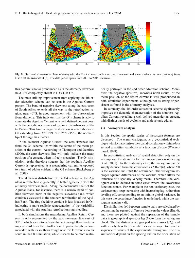
Fig. 9. Sea level skewness (colour scheme) with the black contour indicating zero skewness and mean surface currents (vectors) fromHYCOM O2 (a) and O4 (b). The data period spans from 2001 to 2006, inclusive.

this pattern is not as pronounced as in the altimetry skewnessfield, it is completely absent in HYCOM O2.The most striking improvement from applying the 4th or-

der advection scheme can be seen in the Agulhas Currentproper. The band of negative skewness along the east coastof South Africa extends all the way to the retroflection re-gion, near 40◦ S, in good agreement with the observationsfrom altimetry. This indicates that the O4 scheme is able tosimulate the Agulhas Current as a well defined current core,with the periodic occurrence of cyclonic disturbances or Na-tal Pulses. This band of negative skewness is much shorter inO2 extending from 32◦ E/29◦ S to 25◦ E/35◦ S, the northerntip of the Agulhas Plateau.In the southern Agulhas Current the zero skewness line

from the O4 scheme lies within the centre of the mean po-sition of the current. According to Thompson and Demirov(2006), the zero skewness line will only indicate the meanposition of a current, when it freely meanders. The O4 sim-ulation results therefore suggest that the southern AgulhasCurrent is represented as a meandering current, as opposedto a train of eddies evident in the O2 scheme (Backeberg etal., 2008).The skewness distribution of the O4 scheme at the Ag-

ulhas retroflection is generally in better agreement with thealtimetry skewness field. Along the continental shelf of theAgulhas Bank, for instance, there is a narrow band of pos-itive skewness north of the negative skewness band, whichcontinues westward at the southern termination of the Agul-has Bank. The ring shedding corridor is less focussed in O4,indicating a more realistic representation of the variabilityassociated with the Agulhas retroflection ring shedding.In both simulations the meandering Agulhas Return Cur-

rent is only represented by the zero skewness line east of30◦ E, which seems to indicate that not enough flow is return-ing eastward from the retroflection. In particular, the secondmeander, with its southern trough near 35◦ E extends too farsouth in the O4 simulation, while it seems to be more realis-

tically portrayed in the 2nd order advection scheme. More-over, the negative (positive) skewness north (south) of themean position of the return current is well pronounced inboth simulation experiments, although not as strong or per-sistent as found in the altimetry analyses.In summary, the 4th order advection scheme significantly

improves the dynamic characterisation of the southern Ag-ulhas Current, revealing a well-defined meandering current,with distinct bands of cyclonic and anticyclonic eddies.

4.3 Variogram analysis

In this Section the spatial scales of mesoscale features arediscussed. The (semi-)variogram, is a geostatistical tech-nique which characterises the spatial correlation within a dataset and quantifies variability as a function of scale (Wacker-nagel, 1998).In geostatistics, analyses of spatial data often rely on the

assumption of stationarity for the random process (Gneitinget al., 2001). In the stationary case, the variogram can besimply deduced from the covariance as C0–C(h), where C0is the variance and C(h) the covariance. The variogram av-erages squared differences of the variable, which filters theinfluence of a spatially varying mean. Therefore, the vari-ogram can be defined in some cases where the covariancefunction cannot. For example in the non-stationary case, thevariance may keep increasing with increasing lag, rather thanleveling off, corresponding to an infinite global variance. Inthis case the covariance function is undefined, while the var-iogram remains valid.Dissimilarities (γ ) between sample pairs are calculated by

computing the squared difference between the values (Eq. 4),and these are plotted against the separation of the samplepairs in geographical space, or lag (h), to form the variogramcloud. The lag distances are grouped into classes (Hk), andwithin each class the dissimilarities are averaged to form thesequence of values of the experimental variogram. The dis-similarities depend on the spacing and on the orientation of



the point pair described by the lag vector, and because it is asquared quantity, the order in which the points in space areconsidered does not come into play. Therefore the variogramis symmetric with respect to h.

γ (Hk)=12nc

nc∑

α=1(η(xα+h)−η(xα))2 with h ε Hk (4)

nc are all the point pairs that can be linked by a vector, h. Theaverage dissimilarity with respect to a vector class within aspecific intervalHk , is a value of the experimental variogramγ (Hk).Usually the average dissimilarity between values increases

with distance between point pairs, as near samples tend to bemore alike. If the variable is stationary, at large distancesbetween point pairs the experimental variogram may reacha sill, its maximum. When this occurs the expression con-verges to twice the variance, therefore dividing by 2 meansthat the sill approximates the variance within the data. Atscales exceeding the natural scale of the phenomena in ques-tion, harmonic effects may be noted, in which the variogrampeaks and dips at lag distances that are multiples of the natu-ral scale, this is known as cyclicity.An abrupt change of the slope of the dissimilarity func-

tion at a specific scale indicates that an intermediate level ofvariation has been reached, this is known as the range. Itidentifies the distance from the origin where the variogramreaches its maximum value (the sill), at which point the sam-pled variable exhibits its maximum variance.The behaviour of the variogram near the origin is impor-

tant to note, it characterises the very small scales within adataset and indicates the type of continuity of the variable:differentiable, continuous but not differentiable, or discon-tinuous. A discontinuous variogram at the origin is known asa nugget effect, which indicates that the values of the vari-ables change abruptly at very small scales, it may also arisewhen data is sparse or from measurement error.A theoretical curve is fitted to the variogram in order to

attribute a physical meaning to them. The fit is done by eye,because emphasis is not placed on how well the variogramfunction fits the the sequence points, but rather what typeof continuity is assumed near the origin. The fit thereforeimplies an interpretation of the behaviour of the variogram atthe origin and its behaviour at large lag distances.

4.3.1 Comparison to a spatial fourier analysis

A spatial Fourier and variogram analysis of modelled SLAdata (HYCOM O2) are compared in order to confirm for anoceanographic application, that the variogram indicates thescale up to which a spatial correlation exists between datapoints, thus giving an indication of the size of mesoscale fea-tures. The comparison is done for modelled SLA data alonga section in the Mozambique Channel where large anticy-clonic eddies, up to 300 km in diameter, are known to occurfrequently (HYCOM O2; Backeberg et al., 2008).

Figure 10a is the time averaged spatial FFT spectrum forthe modelled SLA data along the section indicated in Fig. 9a.Notice the peak near Lw

∼=560 km, which for a Fourier anal-ysis typically corresponds to two eddies (cyclonic and an-ticyclonic) with diameters of about 280 km, in agreementwith the simulated eddies observed in HYCOM O2 for theMozambique Channel (Backeberg et al., 2008).The blue curve (Fig. 10b) indicates the corresponding ex-

perimental variogram calculated using Eq. (4), and the redcurve is the theoretical variogram fitted to the sequence(Eq. 5), which in this case is a combination of a Gaussianand a cosine function. Other functions were tested (cardinalsine, cubic, exponential) with less success.

γ (h)=Cg[1−exp(−h2

a2g)]+Cc[1−cos

2πh

ac] (5)

C is the amplitude of the Gaussian/cosine function, h thedistance between points and a the range, or radius. In Eq. (5)the subscripts g and c refer to the Gaussian and cosine vari-ables, respectively. Note that in a Gaussian model the rangeag corresponds to a length scale of ag×2.5, which in thiscase is 275 km (ag=110 km).Mozambique Channel eddies in HYCOM O2 are all of

very similar sizes. Therefore, the typical mesoscale size in-dicated by the Fourier analysis should be of a similar size tothe maximum mesoscale estimated by the variogram. In thiscase, the mesoscale estimate from the variogram is 275 kmand the estimate from the Fourier analysis is 280 km, in goodagreement with each other as expected.In addition to this, the combined Gaussian and cosine fit

indicates a mixture of periodic (cosine) and other (Gaussian)signals. Here the periodic signal suggests a succession of ed-dies. The cosine range (ac=90 km) indicates that successiveeddies are typically ∼560 km (ac×2π ) apart.Both the spatial Fourier and variogram analyses reflect the

whole range of spatial scales related to mesoscale currentsfor a given region. Therefore it may be prudent to refer to“mesoscale features” rather than “eddies” when discussingthese results. However, due to the dominance of anticycloniceddies (in HYCOM O2) in the Mozambique Channel it maybe safe to conclude that these results provide an indicationof the typical (Fourier) and maximum (variogram) eddy di-ameters. For consistency, discussions hereafter will refer to“mesoscale features” only, and these are defined to includeboth eddies and meanders in mesoscale currents.The information contained in a variogram is in principle

equivalent to that contained in a Fourier transform, but thevariogram is more practical for testing the stationarity ofa variable and for examining small scales. In addition tothis the Fourier transform relies on the assumption that thedata domain is periodic rather than infinite. Furthermore,when calculating the experimental variogram the data doesnot need to be preprocessed. Before calculating the Fourier



Fig. 10. Spatial FFT spectrum (a) and variogram analysis (b) of model SLA data from HYCOM O2 along a section in the MozambiqueChannel. The section data was extracted from gridded data and interpolated to 10 km.

transform, trends in the data have to be removed, and taper-ing functions need to be applied at the edges. Moreover, thephysical meaning of the semivariance is easy to interpret. Inthe case of mesoscale variability in the ocean, it representsthe amplitude of the differences, and like eddy kinetic en-ergy, high values represent regions with high mesoscale vari-ability. The major advantage of the variogram, is that it iseasy to calculate, requiring only a few lines of code.These results confirm that the variogram indeed provides

an indication of the size of mesoscale features for a given re-gion, and in addition to this is able to determine the presenceof periodic signals, as well as comparable magnitudes of thevariance.

4.3.2 Quantifying spatial scales of mesoscale variability

To quantify the spatial scale of mesoscale variability in keyregions of the greater Agulhas Current system, three sectionswere defined along which SLA data from Aviso, HYCOMO2 and HYCOM O4 was extracted (see Figs. 8 and 9).The Mozambique Channel section, extending southward

from 43◦ E/14◦ S to 30◦ E/33.5◦ S, was chosen to repre-sent the path along which predominantly anticyclonic eddiespropagate southward from the Mozambique Channel towardthe northern Agulhas Current. This path can be clearly iden-tified in both HYCOM O2 and O4 simulations, and is alsoevident in the altimetry field.The Aviso SLA experimental variogram (Fig. 11a, left)

was fitted with a Gaussian function (the first term in Eq. 5),indicating that a maximum variance (or sill) of 355 cm2 isreached at a radius (or range) of 150 km. This suggests thatmesoscale features (eddies or meanders) along this sectionhave diameters up to 375 km, somewhat larger than previ-ously documented.As discussed previously (Sect. 4.3.1), the HYCOM O2

variogram (Fig. 11, middle) was fitted with a curve com-bining a Gaussian and cosine function (Eq. 5). The respec-tive Gaussian and cosine ranges, (ag and ac) indicate that,

contrary to previous findings (Backeberg et al., 2008), theMozambique Channel eddies in HYCOMO2 are smaller andless intense than in reality, with diameters of 275 km, and asemivariance 60% less than observed from altimetry. In ad-dition to this the periodicity, with successive eddies∼560 km(ac×2π ) apart, is not evident in the altimetry SLA section,indicating that the formation of eddies in the O2 simulationis too regular/periodic.Applying the 4th order advection scheme in HYCOM im-

proves some of the deficiencies of the O2 scheme in theMozambique Channel. The amplitude of the Gaussian sill(Cg) is much higher, and the range has increased to 140 km,corresponding to a diameter of 350 km, in better agreementwith the altimetry observations. There is also some improve-ment in the (artificial) periodicity, in that the amplitude of thecosine function (Cc) is slightly lower, suggesting a reductionof the periodicity.The second section extends from 32◦ E/30◦ S along the

South African east coast toward the retroflection region at20◦ E/39◦ S and lies within a band of negative skewnessthought to be associated with periodic cyclonic disturbancesor Natal Pulses.The Aviso variogram analysis, with Cc=220 cm2 and

ac=125 km, here indicates mesoscale diameters of up to312.5 km, in agreement with the documented scale of the Ag-ulhas retroflection loop (340 km; Lutjeharms and van Balle-gooyen, 1988).The amplitude of the sill in O2 is much higher

(Cc=450 cm2), with a shorter range (ag=100 km) corre-sponding to diameters of 250 km. A periodicity of 80 km(corresponding to eddies ∼500 km apart) confirms the suc-cessive train of eddies simulated in O2.The HYCOM O4 variogram is in much better agreement

with the altimetry, and no periodicity is evident. A Gaussianfunction provides the theoretical fit. The amplitude of the sillis slightly higher, but the range of 125 km is in good agree-ment with the altimetry. A train of eddies (as in O2) will



: 21

Fig. 11. Variogram analysis for Aviso (left column), HYCOM O2 (middle column) and HYCOM O4 (right column). SLA data wasextracted from gridded data along sections for the Mozambique Channel (a), Agulhas Current (b) and Agulhas Ring shedding corridor (c)and interpolated to 10 km. See straight black lines in Figures 8a and 9.Fig. 11. Variogram analysis for Aviso (left column), HYCOM O2 (middle column) and HYCOM O4 (right column). SLA data was

extracted from gridded data along sections for the Mozambique Channel (a), Agulhas Current (b) and Agulhas Ring shedding corridor (c)and interpolated to 10 km. See straight black lines in Figs. 8a and 9.

result in a variogram with a higher variance at the sill, dueto the enhanced variability associated with an eddy field, butwith a smaller spatial scale compared to a well defined cur-rent extending southwestward with a large retroflection loopat its termination, as in Aviso and O4. This result presentsan additional indication that the O4 scheme provides a muchmore realistic simulation of the southern Agulhas Current.From the skewness analysis two sections were defined

in the altimetry for the northwestward passage of AgulhasRings. The first (solid line, Fig. 11c, left) corresponding tothe track along which rings seem to preferentially propagatein HYCOM (Fig. 9) and the second where according to theskewness field from altimetry (Fig. 8), predominantly anticy-clonic eddies are found in the observations (dashed line).The Aviso variogram shows that the northern section has a

variance of 620 cm2, with a scale of 140 km, correspondingto diameters of 350 km. The variance in the southern sectionis 40% lower, but the length scales are similar (135 km cor-responding to a diameter of 337.5 km). This indicates, thateddies shed from the retroflection tend to preferentially prop-agate along the northern track, and that the altimetry skew-ness field is unable to indicate this path as pointed out byThompson and Demirov (2006). Note that Agulhas Ringshave been documented to have diameters of up to 320 km(Lutjeharms and van Ballegooyen, 1988), in good agreementwith the variogram analysis.While in both model simulations the spatial scales are in

good agreement with the altimetry observations, the ampli-

tude of the variance in O2 is too large. A periodic (cosine)signal is also evident in both simulations, suggesting an arti-ficial regularity of Agulhas Ring shedding. This amplitude issomewhat lower in the O4 scheme.In conclusion, using the variogram tool, the spatial scales

of mesoscale features for three sections in the greater Agul-has Current system were quantified. In addition to this, thevariogram analysis, provides an objective tool for compar-ing and validating the two model simulations. It was ableto identify (unrealistic) periodic signals in the model simu-lations, as well as provide a good quantitative comparisonof the scales of the ocean features. A major improvementof the O4 simulation is that the periodicity evident in all thesections for the O2 scheme, is reduced in the MozambiqueChannel and ring shedding corridor, and significantly, absentfor the section through the Agulhas Current. Moreover, thespatial scales and amplitudes of the variances in HYCOM us-ing the 4th order advection scheme are much more realistic,and in better agreement with the altimetry observations.

5 Conclusions

From this inter-comparison of the two numerical advectionschemes in HYCOM it was clearly shown that applyinghigher order numerics (the 4th order momentum advectionscheme) significantly improve the model simulation of thegreater Agulhas Current regime.



The most significant improvement in the O4 simulationis the change in the southern Agulhas Current, from a trainof successive eddies, to a well-defined meandering current.Stronger poleward transports and a much improved verticalstructure of the Agulhas Current near 32◦ S in HYCOMO4 isevident. These improvements may contribute toward a bet-ter southwestward penetration of the temperature field, andimplies a stronger leakage of warm, saline Indian Ocean wa-ters into the South Atlantic Ocean vital for the MeridionalOverturning Circulation.Satellite altimetry measurements of the sea surface are

used in model validation techniques. The sea surface heightvariations, sea level skewness and variogram analyses quan-tify the improvements evident in the simulation, as wellas providing some new perspectives in terms of studyingmesoscale variability in the ocean.Sea level skewness was shown to be an ideal tool for study-

ing flows with meanders that become unstable and changeinto eddies. In an eddy field it is able to distinguish betweena preference for cyclonic or anticyclonic rotation. The zeroskewness line in the southern Agulhas Current confirms thatthroughout the O4 model simulation, the current is repre-sented as a well defined meandering current.The variogram analysis confirms that the O4 scheme sim-

ulates more realistic scales and variances of mesoscale fea-tures. Additionally, it is able to identify (unrealistic) periodicsignals such as too regular Mozambique Channel eddies andsuccessive eddies in the southern Agulhas Current, which arepronounced deficiencies of the O2 scheme.Finally, the Agulhas Current transport, and hence the Indo-

Atlantic inter-ocean exchange, is sensitive to mesoscale fea-tures that originate upstream in the source regions. HYCOMO4, in particular with the improved simulation of the south-ern Agulhas Current, is well suited for application in furtherstudies of this exchange.

Acknowledgements. We would like to thank the team at theMohn-Sverdrup Center for their technical support, in particularfor the implementation of the higher order advection scheme inAGULHAS HYCOM. We would also like to acknowledge thereviewers for their cunstructive review of our work, in particular forsuggesting the inclusion of a vorticity analysis. This work has beensupported by the Mohn-Sverdrup Center for Global Ocean Studiesand Operational Oceanography, through a private donation fromTrond Mohn C/O Frank Mohn AS, Bergen, Norway, and a grant forCPU time from the Norwegian Super-computing (NOTUR) project.We gratefully acknowledge funding from the National ResearchFoundation of South Africa. L. Bertino and J. A. Johannessenacknowledge partial funding from the MERSEA integrated project(number SIP-CT-2003-502885) from the European Commission.We extend our kind thanks to H. L. Bryden for providing thegridded data from the Agulhas Current mooring (Fig. 5b). Weare also grateful for the data supply from CNES, Remote SensingSystems and NOAA/OAR/ESRL PSD.

Edited by: E. J. M. Delhez

References

Backeberg, B. C., Johannessen, J. A., Bertino, L., and Reason, C.J.: The greater Agulhas Current system: An integrated study ofits mesoscale variability, Journal of Operational Oceanography,1(1), 29–44, 2008.

Barnier, B., Madec, M., Pendruff, T., Molines, J.-M., Treguier, A.-M., Sommer, J. L., Beckmann, A., Biastoch, A., Bnning, C.,Dengg, J., Derval, C., Durand, E., Gulev, S., Remy, E., Talandier,C., Theetten, S., Maltrud, M., McClean, J., and DeCuevas, B.:Impact of partial steps and momentum advection schemes ina global ocean circulation model at eddy permitting resolution,Ocean Dynam., 56(5–6), 543–567, 2006.

Bentsen, M., Evensen, G., Drange, H., and Jenkins, A. D.: Coordi-nate transformation on a sphere using conformal mapping, Mon.Weather Rev., 127, 2733–2740, 1999.

Biastoch, A. and Krauss, W.: The role of mesoscale eddies in thesource regions of the Agulhas Current, J. Phys. Oceanogr., 29,2303–2317, 1999.

Bleck, R.: An oceanic general circulation model framed in hy-brid isopycnic-Cartesian coordinates, Ocean Model., 37, 55–88,2002.

Bleck, R.: On the use of hybrid vertical coordinates in ocean cir-culation modeling, in: Ocean Weather Forecasting, edited by:Chassignet, E. P. and Verron, J., Springer, Netherlands, 109–126,2006.

Bleck, R. and Smith, L.: A wind-driven isopycnic coordinate modelof the North Atlantic and Equatorial Atlantic Ocean. 1: Modeldevelopment and supporting experiments, J. Geophys. Res., 95,3273–3285, 1990.

Boebel, O., Rossby, T., Lutjeharms, J. R. E., Zenk, W., and Barron,C.: Path and variability of the Agulhas Return Current, Deep-SeaRes. (II Top. Stud. Oceanogr.), 50, 35–56, 2003.

Leonard, B. P.: A stable and accurate convective modelling proce-dure based on quadratic upstream interpolation, Comp. MethodsAppl. Mech. Eng., 19, 59–98, 1979.

Browning, G. L. and Kreiss, H. O.: Initialization of the shallowwater equations with open boundaries by the bounded derivativemethod, Tellus, 34, 334–351, 1982.

Browning, G. L. and Kreiss, H. O.: Scaling and computation ofsmooth atmospheric motions, Tellus A, 38, 295–313, 1986.

Bryden, H. L., Beal, L. M., and Duncan, L. M.: Structure andTransport of the Agulhas Current and Its Temporal Variability,J. Oceanogr., 61, 479–492, 2005.

Bryden et al., Bacon, S., Beal, L. M., Bonner, R. N., et al.: Ag-ulhas Current Experiment, Cruise Report No. 249, Institute ofOceanographic Sciences, Wormley, 85 pp., 1995.

Davies, H. C.: Limitations of some common lateral boundaryschemes used in NWP models, Mon. Weather Rev., 111, 1002–1012, 1983.

de Ruijter, W. P. M., Ridderinkhof, H., Lutjeharms, J. R. E.,Schouten, M. W., and Veth, C.: Observations of the flow in theMozambique Channel, Geophys. Res. Lett., 29(10), 1502–1504,2002.

de Ruijter, W. P. M., van Leeuwen, P. J., and Lutjeharms, J. R. E.:Generation and Evolution of Natal Pulses: Solitary Meanders inthe Agulhas Current, J. Phys. Oceanogr., 29, 3043–3055, 1999.

Gneiting, T., Sasvari, Z., and Schlather, M.: Analogies and corre-spondences between variograms and covariance functions, Adv.Appl. Prob., 33, 617–630, 2001.



Grundlingh, M. L.: On the course of the Agulhas Current, S. Afr.Geograph. J., 65, 49–57, 1983.

Le Traon, P.-Y.: Satellite oceanography for ocean forecasting, in:Ocean Forecasting, edited by: Pinardi, N. and Woods, J. D.,Springer, New York, USA, 19–36, 2002.

Legates, D. and Willmott, C.: Mean seasonal and spatial variabilityin gauge-corrected, global precipitation, J. Clim., 10, 111–127,1990.

Lutjeharms, J. R. E. and Roberts, H. R.: The Natal Pulse: An ex-treme transient on the Agulhas Current, J. Geophys. Res., 93,631–645, 1988.

Lutjeharms, J. R. E. and Valentine, H. R.: Southern Ocean thermalfronts south of Africa, Deep-Sea Res., 31(12), 1461–1475, 1984.

Lutjeharms, J. R. E. and van Ballegooyen, R. C.: The retroflec-tion of the Agulhas Current, J. Phys. Oceanogr., 18, 1570–1583,1988.

Matano, R. P. and Beier, E. J.: A kinematic analysis of the In-dian/Atlantic interocean exchange, Deep-Sea Res. Pt. II , 50,229–249, 2003.

Morel, Y., Darr, D., and Tailandier, C.: The stability of coastal up-welling and downwelling currents, J. Phys. Oceanogr., 36, 875–896, 2006.

Reynolds, R. W. (1988): A real-time global sea surface temperatureanalysis, J. Climate, 1, 75–86, 1988.

Reynolds, R. W. and Marsico, D. C.: An improved real-time globalsea surface temperature analysis, J. Climate, 7, 929–948, 1994.

Reynolds, R. W., Rayner, N. A., Smith, T. M., Stokes, D. C., andWang, W.: An improved in situ and satellite sst analysis for cli-mate, J. Climate, 15, 1609–1625, 2002.

Richardson, P. L. and Garzoli, S. L.: Characteristics of intermediatewater flow in the Benguela current as measured with RAFOSfloats, Deep-Sea Res. Pt. II, 50, 87–118 2003.

Rio, M.-H., and Hernandez, F.: A mean dynamic topography com-puted over the world ocean from altimetry, in situ measure-ments, and a geoid model, J. Geophys. Res., 109, C12032,doi:10.1029/2003JC002226, 2004.

Rio, M.-H., Schaeffer, P., Lemoine, J.-M., and Hernandez, F.: Esti-mation of the ocean mean dynamic topography through the com-bination of altimetric data, in situ measurements and grace geoid,in Proceedings of the GOCINA international workshop, Luxem-bourg, 2005.

Rouault, M. and Lutjeharms, J. R. E.: Estimation of sea-surfacetemperature around southern Africa from satellite-derived mi-crowave observations, S. Afr. J. Sci., 99, 489–494, 2003.

Sætre, R. and da Silva, A. J.: The circulation of the MozambiqueChannel, Deep-Sea Res., 31, 485–508, 1984.

Sanderson, B. G.: Order and resolution for computational oceandynamics, J. Phys. Oceanogr., 28, 1271–1286, 1998.

Schouten, M. W., de Ruijter, W. P. M., and van Leeuwen, P. J.:Upstream control of Agulhas Ring shedding, J. Geophys. Res.,107(C8), 3109–3120, 2002.

Siedler, G., Rouault, M., Biastoch A., Backeberg, B., Reason, C.J. C., and Lutjeharms J. R. E.: Modes of the southern extensionof the East Madagascar Current, J. Geophys. Res., 114, C01005,doi:10.1029/2008JC004921, 2009.

Slutz, R., Hiscox, S. L. J., Woodruff, S., Jenne, R., Joseph, D.,Steurer, P., and Elms, J.: Comprehensive ocean-atmospheredataset, Release 1. Tech. Rep. NTIS PB86-105723, NOAA En-vironmental Research Laboratories, Climate Research Program,Boulder, CO, 1985.

Teague, W. J., Carron, M., and Hogan, P. J.: A comparison betweenthe Generalized Digital Environmental Model and Levitus clima-tologies, J. Geophys. Res., 95(C5), 7167–7183, 1990.

Thompson, K. R. and Demirov, E.: Skewness of sea level vari-ability of the world’s oceans, J. Geophys. Res., 111(C05005),doi:10.1029/2004JC002839, 2006.

Treguier, A. M., Boebel, O., Barnier, B., and Madec, G.: Agulhaseddy fluxes in a 1/6◦ Atlantic model, Deep-Sea Res. Pt. II, 50,251–280, 2003.

Uppala, S. M., Kallberg, P. W., Simmons, A. J., Andrae, U., DaCosta Bechtold, V., Fiorino, M., Gibson, J. K., Haseler, J., Her-nandez, A., Kelly, G. A., Li, X., Onogi, K., Saarinen, S., Sokka,N., Allan, R. P., Andersson, E., Arpe, K., Balmaseda, M. A.,Beljaars, A. C. M., Van De Berg, L., Bidlot, J., Bormann, N.,Caires, S., Chevallier, F., Dethof, A., Dragosavac, M., Fisher,M., Fuentes, M., Hagemann, S., Hlm, E., Hoskins, B. J., Isak-sen, L., Janssen, P. A. E. M., Jenne, R., McNally, A. P., Mahfouf,J.-F., Morcrette, J.-J., Rayner, N. A., Saunders, R. W., Simon,P., Sterl, A., Trenberth, K. E., Untch, A., Vasiljevic, D., Viterbo,P., and Woollen, J.: The ERA-40 re-analysis, Q. J. R. Meteorol.Soc., 131(612), 2961–3012, 2005.

Wackernagel, H.: Multivariate geostatistics: An Introduction withApplications, 2nd edn., Springer-Verlag Telos, Berlin, Germany,291 pp., 1998.

Webb, D. J., Cuevas, B. A., and Richmond, C.: Improved advectionschemes for ocean models, J. Atmos. Ocean Tech., 15, 1171–1187, 1998.

Winther, N. G., Morel, Y., and Evensen, G.: Effciency of high ordernumerical schemes for momentum advection, J. Mar. Sys., 67,31–46, 2007.


evaluating two numerical advection schemes in hycom for

Documents