logo

Evaluating Value at Risk using Generalised AsymmetricVolatility Models

by Georgios K. Tsiotas, University of Crete5th CFE

London, 17-19/12, 2011

January 9, 2012

by Georgios K. Tsiotas, University of Crete 5th CFE London, 17-19/12, 2011 Evaluating Value at Risk using Generalised Asymmetric Volatility Models

logo

Stochastic Volatility (SV) ModelsValue at Risk (VaR) in SV models

Testing VaR modelsResults

General Comments

Contents

1 Stochastic Volatility (SV) Models

2 Value at Risk (VaR) in SV models

3 Testing VaR models

4 Results

5 General Comments

by Georgios K. Tsiotas, University of Crete 5th CFE London, 17-19/12, 2011 Evaluating Value at Risk using Generalised Asymmetric Volatility Models

logo

Stochastic Volatility (SV) ModelsValue at Risk (VaR) in SV models

Testing VaR modelsResults

General Comments

Volatility

Why Volatility?

Volatility-Variance as a measure of risk in economics and financial data.Conditional volatility measures time-varying risk (alternative to theBlack-Scholes approach)

How to model Volatility? Stylised facts?

volatility dynamics (clusters)

excess kurtosis

possible mean and volatility asymmetry

by Georgios K. Tsiotas, University of Crete 5th CFE London, 17-19/12, 2011 Evaluating Value at Risk using Generalised Asymmetric Volatility Models

logo

Stochastic Volatility (SV) ModelsValue at Risk (VaR) in SV models

Testing VaR modelsResults

General Comments

Volatility

Why Volatility?

Volatility-Variance as a measure of risk in economics and financial data.Conditional volatility measures time-varying risk (alternative to theBlack-Scholes approach)

How to model Volatility? Stylised facts?

volatility dynamics (clusters)

excess kurtosis

possible mean and volatility asymmetry

by Georgios K. Tsiotas, University of Crete 5th CFE London, 17-19/12, 2011 Evaluating Value at Risk using Generalised Asymmetric Volatility Models

logo

Stochastic Volatility (SV) ModelsValue at Risk (VaR) in SV models

Testing VaR modelsResults

General Comments

Volatility

Plot of the S&P500, DAX 30, and NASDAQ return data series

0 500 1000 1500 2000 2500

−10

−5

05

10

Observations

SP

500

retu

rns

0 500 1000 1500 2000 2500

−5

05

10

Observations

DA

X30

ret

urns

0 500 1000 1500 2000 2500

−10

−5

05

10

Observations

NA

SD

AQ

ret

urns

by Georgios K. Tsiotas, University of Crete 5th CFE London, 17-19/12, 2011 Evaluating Value at Risk using Generalised Asymmetric Volatility Models

logo

Stochastic Volatility (SV) ModelsValue at Risk (VaR) in SV models

Testing VaR modelsResults

General Comments

Volatility

Table: Summary statistics of return index series financial series

statisticsskewness ex.kurtosis jarque bera test asymmetry test

sp500 -0.1176 4.955 6655.394(< 2.2e-16) 89.1320(< 2.2e-16)dax30 -0.045 1.266 1915.837(< 2.2e-16) 76.4619(< 2.2e-16)nasdaq -0.043 1.475 2115.423(< 2.2e-16) 79.2918(< 2.2e-16)

by Georgios K. Tsiotas, University of Crete 5th CFE London, 17-19/12, 2011 Evaluating Value at Risk using Generalised Asymmetric Volatility Models

logo

Stochastic Volatility (SV) ModelsValue at Risk (VaR) in SV models

Testing VaR modelsResults

General Comments

Modelling Volatility Models

Conditionally Volatility models [Engle, 1986; Bollerslev, 1992]

ARCH and GARCH models describe conditional volatility. E.g GARCH(1,1):

yt = α+ β1yt−1 + · · · + βpyt−p + ǫt , ǫt ∼ Niid(0,1)

σ2t = c + γǫ2

t−1 + δσ2t−1

Stochastic Volatility (SV) models [Shephard, 1994; Shephard el. al., 1997]

yt = σt · ǫt = eht/2 · ǫt , t = 1, . . . ,T

ht+1 = logσ2t+1 = µ+ φ(ht − µ) + τ · ut ,

(ǫt , ut) ∼ Niid(0, I), µ ∈ ℜ, φ ∈ (−1,1), τ ∈ (0,+∞)

by Georgios K. Tsiotas, University of Crete 5th CFE London, 17-19/12, 2011 Evaluating Value at Risk using Generalised Asymmetric Volatility Models

logo

Stochastic Volatility (SV) ModelsValue at Risk (VaR) in SV models

Testing VaR modelsResults

General Comments

Modelling Volatility Models

Conditionally Volatility models [Engle, 1986; Bollerslev, 1992]

ARCH and GARCH models describe conditional volatility. E.g GARCH(1,1):

yt = α+ β1yt−1 + · · · + βpyt−p + ǫt , ǫt ∼ Niid(0,1)

σ2t = c + γǫ2

t−1 + δσ2t−1

Stochastic Volatility (SV) models [Shephard, 1994; Shephard el. al., 1997]

yt = σt · ǫt = eht/2 · ǫt , t = 1, . . . ,T

ht+1 = logσ2t+1 = µ+ φ(ht − µ) + τ · ut ,

(ǫt , ut) ∼ Niid(0, I), µ ∈ ℜ, φ ∈ (−1,1), τ ∈ (0,+∞)

by Georgios K. Tsiotas, University of Crete 5th CFE London, 17-19/12, 2011 Evaluating Value at Risk using Generalised Asymmetric Volatility Models

logo

Stochastic Volatility (SV) ModelsValue at Risk (VaR) in SV models

Testing VaR modelsResults

General Comments

Stochastic Volatility Models

Stochastic Volatility (cont.)

unobservable volatility

natural way to estimate volatility as a latent process

Other SV models

Asymmetric SV (ASV) model [Harvey and Shephard, 1996]

yt = eht/2 · ǫt , ht+1 = µ+ φ(ht − µ) + τ · ut+1,

„

ǫt

ut+1

«

∼ Niid(0,Σ), Σ =

„

1 ρρ 1

«

.

With ρ is negative then a negative shock in the return series will beassociated with higher contemporaneous volatility shocks.

by Georgios K. Tsiotas, University of Crete 5th CFE London, 17-19/12, 2011 Evaluating Value at Risk using Generalised Asymmetric Volatility Models

logo

Stochastic Volatility (SV) ModelsValue at Risk (VaR) in SV models

Testing VaR modelsResults

General Comments

Stochastic Volatility Models

Stochastic Volatility (cont.)

unobservable volatility

natural way to estimate volatility as a latent process

Other SV models

Asymmetric SV (ASV) model [Harvey and Shephard, 1996]

yt = eht/2 · ǫt , ht+1 = µ+ φ(ht − µ) + τ · ut+1,

„

ǫt

ut+1

«

∼ Niid(0,Σ), Σ =

„

1 ρρ 1

«

.

With ρ is negative then a negative shock in the return series will beassociated with higher contemporaneous volatility shocks.

by Georgios K. Tsiotas, University of Crete 5th CFE London, 17-19/12, 2011 Evaluating Value at Risk using Generalised Asymmetric Volatility Models

logo

Stochastic Volatility (SV) ModelsValue at Risk (VaR) in SV models

Testing VaR modelsResults

General Comments

Stochastic Volatility Models

Generalised SV models

The noncentral-t SV (SV-nct) model [Johnson et al., 1995], [Tsiotas, 2010]

yt = eht/2 · ǫt ≡ eht/2 ·p

ζt (zt + δ),

ǫt ∼ t∗k,δ(0, 1), ζt ∼ IG(k/2, 2/k), zt ∼ N(0, 1)

where ǫt is a standardised nct random variable with k degrees of freedom andnoncentrality parameter δ. Here, ǫt = µnct +

√ζt(zt + δ) · σnct , with ǫt ∼ tk,δ a nct

random variable with mean and variance components given by:

µnct = δ

r

k

2

Γ((k − 1)/2)

Γ(k/2),

and

σ2nct =

k(1 + δ2)

k − 2− δ2k

2

„

Γ((k − 1)/2)

Γ(k/2)

«2

.

modelling both skewness and excess kurtosis

generalised version of the t-distributed SV model

data justification

by Georgios K. Tsiotas, University of Crete 5th CFE London, 17-19/12, 2011 Evaluating Value at Risk using Generalised Asymmetric Volatility Models

logo

Stochastic Volatility (SV) ModelsValue at Risk (VaR) in SV models

Testing VaR modelsResults

General Comments

Stochastic Volatility Models

Generalised SV models (cont.)

The skewed normal SV (SV-sn) model [Azzalini, 1986], [Bazan et al., 2006],[Tsiotas, 2010]

yt = eht/2 · ǫt ≡ eht/2 · (δvt +p

1 − δ2zt ),

vt ∼ HNiid(0,1), zt ∼ Niid(0,1), ǫt ∼ SN(λ),

where ǫt = µsn + ǫt · σsn with ǫt ∼ SN(µsn, σ2sn, λ) a SN random variable with λ

the skewness parameter and δ = λ/(1 + λ2)1/2. The mean and variancecomponents of ǫt are given by:

µsn =p

2/πδ,

andσ2

sn = (1 − 2δ2/π),

respectively.

by Georgios K. Tsiotas, University of Crete 5th CFE London, 17-19/12, 2011 Evaluating Value at Risk using Generalised Asymmetric Volatility Models

logo

Stochastic Volatility (SV) ModelsValue at Risk (VaR) in SV models

Testing VaR modelsResults

General Comments

Stochastic Volatility Models

Generalised SV models (cont.)

The skewed t-distributed SV (SV-st) model [Lin et al., 2007], [Tsiotas, 2010]

yt = eht/2 · ǫt ≡ eht/2 ·p

ζt · (δvt +p

1 − δ2zt ),

vt ∼ HNiid(0,1), zt ∼ Niid(0,1), ζt ∼ IG(k/2, 2/k), ǫt ∼ SN(λ),

where ǫt = µst + ǫt ·√ζt · σst with ǫt ∼ ST (µst , σ

2st , λ, k) a ST random variable

with k degrees of freedom, λ skewness parameter, and mean and variancecomponents given by:

µst = δ(k/π)1/2Γ((k − 1)/2)

Γ(k/2),

and

σ2st =

kk − 2

,

respectively. Here, when δ equals zero, our model reduces to the SV-t one.

by Georgios K. Tsiotas, University of Crete 5th CFE London, 17-19/12, 2011 Evaluating Value at Risk using Generalised Asymmetric Volatility Models

logo

Stochastic Volatility (SV) ModelsValue at Risk (VaR) in SV models

Testing VaR modelsResults

General Comments

Stochastic Volatility Models

Generalised Asymmetric SV models [Tsiotas, 2010]

The Asymmetric SV-nct (ASV-nct) model, with:

ht+1 = µ+ φ(ht − µ) + ρτ(ζ−1/2t e−ht/2yt − δ) + τ

q

1 − ρ2ηt+1,

where ηt+1 = [ut+1 − ρ(ζ−1/2t ǫt − δ)]/

p

1 − ρ2.

The Asymmetric SV-sn (ASV-sn) model, with:

ht+1 = µ+ φ(ht − µ) + ρτ(1 − δ2)−1/2(e−ht/2yt − δvt ) + τ

q

1 − ρ2ηt+1,

where ηt+1 = (ut+1 − ρ(1 − δ2)−1/2(ǫt − δvt )/p

1 − ρ2.

The Asymmetric SV-st (ASV-st) model, with:

ht+1 = µ+ φ(ht − µ) + ρτζ−1/2t (1 − δ2)−1/2(e−ht/2yt − δvt ) + τ

q

1 − ρ2ηt+1,

where ηt+1 = (ut+1 − ρζ−1/2t (1 − δ2)−1/2(ǫt − λvt )/

p

1 − ρ2.

by Georgios K. Tsiotas, University of Crete 5th CFE London, 17-19/12, 2011 Evaluating Value at Risk using Generalised Asymmetric Volatility Models

logo

Stochastic Volatility (SV) ModelsValue at Risk (VaR) in SV models

Testing VaR modelsResults

General Comments

Bayesian Inference in SV models

MCMC Estimation

MCMC is a method for exploring the posterior distribution in Bayesianinference. We use Gibbs sampler when conditional posterior distributions arestandard distributions, otherwise we employ Metropolis-Hastings [Gelman etal. 2004]

Simulate from posterior densities

1 Single move sampling

p(θ | h, y), p(ht | h−t , θ, y), p(ζt | ζ−t , θ, y,h),

withh = (h1, . . . , hT ), y = (y1, . . . , yT ), ζ = (ζ1, . . . , ζT )

where θ = (µ, φ, τ, k , ρ, δ) and ψ = (θ, h, ζ).2 Priors:

ζt ∼ IG(k/2, 2/k), φ ∼ N(0, 100)I(−1, 1), µ ∼ N(0, 100), ρ ∼ N(0, 100)I(−1, 1),

δ ∼ N(0, 100)I(−1, 1), τ ∼ IG(2.5, 40), k ∼ Exp(.01)I(2,∞).

by Georgios K. Tsiotas, University of Crete 5th CFE London, 17-19/12, 2011 Evaluating Value at Risk using Generalised Asymmetric Volatility Models

logo

Stochastic Volatility (SV) ModelsValue at Risk (VaR) in SV models

Testing VaR modelsResults

General Comments

Bayesian Inference in SV models

MCMC Estimation

MCMC is a method for exploring the posterior distribution in Bayesianinference. We use Gibbs sampler when conditional posterior distributions arestandard distributions, otherwise we employ Metropolis-Hastings [Gelman etal. 2004]

Simulate from posterior densities

1 Single move sampling

p(θ | h, y), p(ht | h−t , θ, y), p(ζt | ζ−t , θ, y,h),

withh = (h1, . . . , hT ), y = (y1, . . . , yT ), ζ = (ζ1, . . . , ζT )

where θ = (µ, φ, τ, k , ρ, δ) and ψ = (θ, h, ζ).2 Priors:

ζt ∼ IG(k/2, 2/k), φ ∼ N(0, 100)I(−1, 1), µ ∼ N(0, 100), ρ ∼ N(0, 100)I(−1, 1),

δ ∼ N(0, 100)I(−1, 1), τ ∼ IG(2.5, 40), k ∼ Exp(.01)I(2,∞).

by Georgios K. Tsiotas, University of Crete 5th CFE London, 17-19/12, 2011 Evaluating Value at Risk using Generalised Asymmetric Volatility Models

logo

Stochastic Volatility (SV) ModelsValue at Risk (VaR) in SV models

Testing VaR modelsResults

General Comments

Bayesian Inference in SV models

MCMC Estimation

MCMC is a method for exploring the posterior distribution in Bayesianinference. We use Gibbs sampler when conditional posterior distributions arestandard distributions, otherwise we employ Metropolis-Hastings [Gelman etal. 2004]

Simulate from posterior densities

1 Single move sampling

p(θ | h, y), p(ht | h−t , θ, y), p(ζt | ζ−t , θ, y,h),

withh = (h1, . . . , hT ), y = (y1, . . . , yT ), ζ = (ζ1, . . . , ζT )

where θ = (µ, φ, τ, k , ρ, δ) and ψ = (θ, h, ζ).2 Priors:

ζt ∼ IG(k/2, 2/k), φ ∼ N(0, 100)I(−1, 1), µ ∼ N(0, 100), ρ ∼ N(0, 100)I(−1, 1),

δ ∼ N(0, 100)I(−1, 1), τ ∼ IG(2.5, 40), k ∼ Exp(.01)I(2,∞).

by Georgios K. Tsiotas, University of Crete 5th CFE London, 17-19/12, 2011 Evaluating Value at Risk using Generalised Asymmetric Volatility Models

logo

Stochastic Volatility (SV) ModelsValue at Risk (VaR) in SV models

Testing VaR modelsResults

General Comments

Contents

1 Stochastic Volatility (SV) Models

2 Value at Risk (VaR) in SV models

3 Testing VaR models

4 Results

5 General Comments

by Georgios K. Tsiotas, University of Crete 5th CFE London, 17-19/12, 2011 Evaluating Value at Risk using Generalised Asymmetric Volatility Models

logo

Stochastic Volatility (SV) ModelsValue at Risk (VaR) in SV models

Testing VaR modelsResults

General Comments

VaR

What is it?

VaR is an α-level quantile of a financial return series or portfolio,

α = P(yt < −VaRt | Yt−1)

expressing the worst expected loss at time t for a given nominal value α.1 Proposed by J.P. Morgan in 1993 and introduced in Basel I for risk

management in 19962 VaR measure says nothing about the expected magnitude of the loss3 Alternatively, Expected Shortfall (ES) expresses the loss on the day

when losses are larger than the VaR

by Georgios K. Tsiotas, University of Crete 5th CFE London, 17-19/12, 2011 Evaluating Value at Risk using Generalised Asymmetric Volatility Models

logo

Stochastic Volatility (SV) ModelsValue at Risk (VaR) in SV models

Testing VaR modelsResults

General Comments

Bayesian VaR estimates

Marginal likelihood is defined as the model’s likelihood function integratedwith respect to all prior information available. This takes the form:

m(y) =

Z

p(y | ψ)π(ψ)dψ.

here ψ = (θ,h). In a similar way, the VaR estimate becomes:

VaRt(α | Yt−1) = {x :

Z x

−∞

p(yt | θ, ht)dytdθdht = α}.

In the MCMC context, due to intructability, each individual VaR is estimatedfrom:

VaRt(α | Yt−1) ≈1J

JX

j=1

VaR(α | Yt−1, θj , hj

t).

for J-MCMC replicated outputs.

by Georgios K. Tsiotas, University of Crete 5th CFE London, 17-19/12, 2011 Evaluating Value at Risk using Generalised Asymmetric Volatility Models

logo

Stochastic Volatility (SV) ModelsValue at Risk (VaR) in SV models

Testing VaR modelsResults

General Comments

Forecast VaR estimates

One-step ahead α quantiles-VaR

VaRnctt+1(α | Yt−1) = tδ,k (α) · σt+1 · σ−1

nct − δ

r

k2

Γ((k − 1)/2)

Γ(k/2)· σt+1 · σ−1

nct

VaRsnt+1(α | Yt−1) = snδ(α) · σt+1 ·

1p

1 − 2δ2/π−

p

2/πδ · 1p

1 − 2δ2/π

VaRstt+1(α | Yt−1) = stk,δ(α) · σt+1 ·

r

k − 2

k− δ

(k/π)1/2Γ((k − 1)/2)

Γ(k/2)· σt+1 ·

r

k − 2

k

by Georgios K. Tsiotas, University of Crete 5th CFE London, 17-19/12, 2011 Evaluating Value at Risk using Generalised Asymmetric Volatility Models

logo

Stochastic Volatility (SV) ModelsValue at Risk (VaR) in SV models

Testing VaR modelsResults

General Comments

Conditional Autoregressive VaR (CARiaR) models

CAViaR models

Estimate quantile directly assuming conditional quantile dependence due tothe presence of of volatility clustering.

Asymmetric slope (AS) CAViaR model

ft(β) = β0 + β1ft−1 + (β3I{yt−1>0} + β4I{yt−1<0}) | yt−1 |

1 Considers VaR dynamics that depend on changing return sign2 Similar in spirit to Exponential and GJR Conditional Volatility models3 Relative good validation results4 Use AS CAViaR as a benchmark model for VaR testing

by Georgios K. Tsiotas, University of Crete 5th CFE London, 17-19/12, 2011 Evaluating Value at Risk using Generalised Asymmetric Volatility Models

logo

Stochastic Volatility (SV) ModelsValue at Risk (VaR) in SV models

Testing VaR modelsResults

General Comments

CAViaR’s estimation objective

Single CAViaR model

Minimising tick-loss function

Lα(et+h) ≡ (α− I{et+h<0}) · et+h

where et+h = yt − ft (β) for a given α.

Combined CAViaR model

et+h = yt − θ0 − θ1ft,1(β2) − θ2ft,2(β2)

1 Consider CAViaR model uncertainty2 Can test a single against alternative combined CAViaR forecasts3 Can apply conditional quantile encompassing test as in [Giacomini and

Komunjer, 2005]4 Parameters θ1 and θ2 not restricted as combination weights [Granger

and Ramanathan, 1984]by Georgios K. Tsiotas, University of Crete 5th CFE London, 17-19/12, 2011 Evaluating Value at Risk using Generalised Asymmetric Volatility Models

logo

Stochastic Volatility (SV) ModelsValue at Risk (VaR) in SV models

Testing VaR modelsResults

General Comments

CAViaR’s estimation

Estimation puzzle

Derive the β parameter estimates via simulation using a quasi-Bayesianestimation (or Laplace type estimation) that uses general statistical criterionfunctions, such as loss functions in place of parametric likelihood functions[Chernozhukov and Hong, 2003].Here, the quasi posterior density of β is proportional to:

p(β) = e−Lα(et+h) × π(β)

1 Can apply Metropolis-Hastings with quasi posteriors2 Alternatively can apply optimization techniques to estimate β

by Georgios K. Tsiotas, University of Crete 5th CFE London, 17-19/12, 2011 Evaluating Value at Risk using Generalised Asymmetric Volatility Models

logo

Stochastic Volatility (SV) ModelsValue at Risk (VaR) in SV models

Testing VaR modelsResults

General Comments

Contents

1 Stochastic Volatility (SV) Models

2 Value at Risk (VaR) in SV models

3 Testing VaR models

4 Results

5 General Comments

by Georgios K. Tsiotas, University of Crete 5th CFE London, 17-19/12, 2011 Evaluating Value at Risk using Generalised Asymmetric Volatility Models

logo

Stochastic Volatility (SV) ModelsValue at Risk (VaR) in SV models

Testing VaR modelsResults

General Comments

Testing the Accuracy of Risk

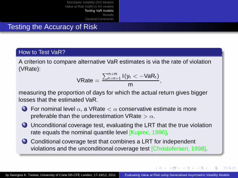
How to Test VaR?

A criterion to compare alternative VaR estimates is via the rate of violation(VRate):

VRate =

Pn+mt=n+1 I(yt < −VaRt)

m,

measuring the proportion of days for which the actual return gives biggerlosses that the estimated VaR.

1 For nominal level α, a VRate < α conservative estimate is morepreferable than the underestimation VRate > α.

2 Unconditional coverage test, evaluating the LRT that the true violationrate equals the nominal quantile level [Kupiec, 1996].

3 Conditional coverage test that combines a LRT for independentviolations and the unconditional coverage test [Christofersen, 1998].

by Georgios K. Tsiotas, University of Crete 5th CFE London, 17-19/12, 2011 Evaluating Value at Risk using Generalised Asymmetric Volatility Models

logo

Stochastic Volatility (SV) ModelsValue at Risk (VaR) in SV models

Testing VaR modelsResults

General Comments

Contents

1 Stochastic Volatility (SV) Models

2 Value at Risk (VaR) in SV models

3 Testing VaR models

4 Results

5 General Comments

by Georgios K. Tsiotas, University of Crete 5th CFE London, 17-19/12, 2011 Evaluating Value at Risk using Generalised Asymmetric Volatility Models

logo

Stochastic Volatility (SV) ModelsValue at Risk (VaR) in SV models

Testing VaR modelsResults

General Comments

Model Validation Results, 5 and 10-step-ahead forecasting

Real Data Series

Sample S&P 500, DAX 30, and NASDAQ indices starting from the 3rd ofApril 2000 and ending on the 6th of April 2010

Out-of-sample (300 obs)-period 27th of January 2009 and the 6th ofApril 2010.

by Georgios K. Tsiotas, University of Crete 5th CFE London, 17-19/12, 2011 Evaluating Value at Risk using Generalised Asymmetric Volatility Models

logo

Stochastic Volatility (SV) ModelsValue at Risk (VaR) in SV models

Testing VaR modelsResults

General Comments

Forecast Evaluation of Conditional VaR

Table: VaR statistics using DAX h = 5 daily return data

α = 0.01models Violations VRate/α LRuc p-value LRcc p-valueSVM 2.00 0.6666 0.3815 0.5368 0.0269 0.8696SVM-nct 3.00 1.00 0.00 1.00 0.0608 0.8052SVM-sn 4.00 1.333 0.3048 0.5808 0.1084 0.7418SVM-st 5.00 1.666 1.121 0.2895 0.1700 0.6800ASV 3.00 1.00 0.00 1.00 0.0404 0.8405ASV-nct 3.00 1.00 0.00 1.00 0.0608 0.8052ASV-sn 3.00 1.00 0.000 1.00 0.06081 0.8052ASV-st 3.00 1.00 0.00 1.00 0.06081 0.8052

α = 0.05SVM 16.00 1.0666 0.0687 0.7931 1.810 0.1784SVM-nct 17.00 1.133 0.2696 0.6035 2.050 0.1521SVM-sn 17.00 1.133 0.2696 0.6035 2.050 0.1521SVM-st 15.00 1.00 0.00 1.00 1.585 0.2080ASV 16.00 1.066 0.0687 0.7931 0.0504 0.8223ASV-nct 16.00 1.066 0.0687 0.7931 0.0504 0.8223ASV-sn 16.00 1.066 0.0687 0.7931 1.810 0.1784ASV-st 16.00 1.066 0.0687 0.7931 1.810 0.1784

by Georgios K. Tsiotas, University of Crete 5th CFE London, 17-19/12, 2011 Evaluating Value at Risk using Generalised Asymmetric Volatility Models

logo

Stochastic Volatility (SV) ModelsValue at Risk (VaR) in SV models

Testing VaR modelsResults

General Comments

Forecast Evaluation of Conditional VaR

Table: VaR statistics using DAX h = 10 daily return data

α = 0.01models Violations VRate/α LRuc p-value LRcc p-valueSVM 4.00 1.333 0.3048 0.5808 0.1084 0.7418SVM-nct 4.00 1.333 0.3048 0.5808 0.1084 0.7418SVM-sn 4.00 1.333 0.3048 0.5808 0.1084 0.7418SVM-st 4.00 1.333 0.3048 0.5808 0.1084 0.7418ASV 4.00 1.333 0.3048 0.5808 0.0812 0.7756ASV-nct 3.00 1.00 0.00 1.00 0.0608 0.8052ASV-sn 4.00 1.333 0.3048 0.5808 0.1084 0.7418ASV-st 3.00 1.00 0.00 1.00 0.0608 0.8052

α = 0.05SVM 16.00 1.0666 0.0687 0.7931 1.810 0.1784SVM-nct 16.00 1.066 0.0687 0.7931 1.810 0.1784SVM-sn 12.00 0.8000 0.6760 0.4109 1.003 0.3163SVM-st 15.00 1.00 0.00 1.00 1.5852 0.2080ASV 17.00 1.1333 0.2696 0.6035 0.0097 0.9212ASV-nct 16.00 1.066 0.0687 0.7931 1.810 0.1784ASV-sn 16.00 1.066 0.0687 0.7931 1.810 0.1784ASV-st 15.00 1.00 0.00 1.00 1.585 0.2080

by Georgios K. Tsiotas, University of Crete 5th CFE London, 17-19/12, 2011 Evaluating Value at Risk using Generalised Asymmetric Volatility Models

logo

Stochastic Volatility (SV) ModelsValue at Risk (VaR) in SV models

Testing VaR modelsResults

General Comments

Forecast Evaluation of Combined Conditional VaR

Table: Combined VaR performance using the DAX data series for 10-step-aheadpredictions

α = 0.01models SV-nct SV-sn SV-st AS AS-nct ASV-sn ASV-stSV 1.33(0.7418) 1.33(0.7418) 1.00(0.8052) 1.33(0.7418) 0.666(0.8696) 1.00(0.8052) 1.33(0.718)SV-nct 1.00(0.8052) 1.33(0.7418) 1.00(0.8052) 1.00(0.8052) 1.333(0.7418) 0.333 (0.9347)SV-sn 1.33(0.7418) 1.00(0.8052) 1.00(0.8052) 0.6666(0.8696) 1.00(0.8052)SV-st 1.33(0.7418) 0.6666(0.8696) 0.3333(0.9347) 1.00(0.8052)AS 1.33(0.7418) 1.333(0.7418) 1.33(0.7418)ASV-nct 1.00(0.8052) 1.33(0.7458)ASV-sn 1.00(0.8052)

α = 0.05models SV-nct SV-sn SV-st AS ASV-nct ASV-sn ASV-stSV 1.00(0.2080) 1.00(0.2080) 0.933(0.6765) 1.00(0.7738) 0.8666(0.6301) 1.00(0.7738) 0.9333(0.240)SV-nct 0.933(0.2407) 0.933(0.6765) 0.933(0.2407) 1.066(0.8725) 1.00(0.2080) 1.066 (0.1784)SV-sn 1.066(0.8725) 1.00(0.2080) 1.00(0.7738) 0.8666(0.2469) 1.00(0.2080)SV-st 1.00(0.2080) 1.00(0.7738) 0.9333(0.2407) 1.00(0.7738)AS 0.933(0.6765) 0.9333(0.2407) 1.00(0.2080)ASV-nct 0.933(0.2470) 0.933(0.2470)ASV-sn 1.066(0.1784)

Note: Entries in each table represent the Violation Rate (VRate) over the nominal α of a row by column combined CaViaR model. Numberswithin parentheses next to each VRate represents the p-values of the Conditional LR test.

by Georgios K. Tsiotas, University of Crete 5th CFE London, 17-19/12, 2011 Evaluating Value at Risk using Generalised Asymmetric Volatility Models

logo

Stochastic Volatility (SV) ModelsValue at Risk (VaR) in SV models

Testing VaR modelsResults

General Comments

Forecast Evaluation of Conditional VaR

Table: VaR statistics using SP500 h = 5 daily return data

α = 0.01models Violations VRate/α LRuc p-value LRcc p-valueSVM 3.00 1.00 0.000 1.00 0.0608 0.8052SVM-nct 3.00 1.00 0.00 1.00 0.0608 0.8052SVM-sn 4.00 1.333 0.3048 0.5808 0.1084 0.7418SVM-st 2.00 0.6666 0.3815 0.5368 0.0269 0.8696ASV 2.00 0.6666 0.3815 0.5368 0.0269 0.8696ASV-nct 3.00 1.00 0.00 1.00 0.0608 0.8052ASV-sn 2.00 0.6666 0.3815 0.5368 0.0269 0.8696ASV-st 3.00 1.00 0.00 1.00 0.0608 0.8052

α = 0.05SVM 17.00 1.13 0.2696 0.6032 2.050 0.1521SVM-nct 15.00 1.00 0.00 1.00 1.585 0.2080SVM-sn 15.00 1.00 0.00 1.00 1.585 0.2080SVM-st 16.00 1.06 0.0687 0.7931 1.810 0.1784ASV 15.00 1.00 0.00 1.00 1.585 0.2080ASV-nct 15.00 1.00 0.00 1.00 1.585 0.2080ASV-sn 16.00 1.066 0.0687 0.7931 1.810 0.1784ASV-st 14.00 0.9333 0.0717 0.7888 0.1740 0.6765

by Georgios K. Tsiotas, University of Crete 5th CFE London, 17-19/12, 2011 Evaluating Value at Risk using Generalised Asymmetric Volatility Models

logo

Stochastic Volatility (SV) ModelsValue at Risk (VaR) in SV models

Testing VaR modelsResults

General Comments

Forecast Evaluation of Conditional VaR

Table: VaR statistics using SP500 h = 10 daily return data

α = 0.01models Violations VRate/α LRuc p-value LRcc p-valueSVM 3.00 1.00 0.00 1.00 0.0608 0.8052SVM-nct 3.00 1.00 0.00 1.00 0.0608 0.8052SVM-sn 3.00 1.00 0.00 1.00 0.0608 0.8052SVM-st 4.00 1.33 0.3048 0.5808 0.1084 0.7418ASV 4.00 1.33 0.3048 0.5808 0.1084 0.7418ASV-nct 3.00 1.00 0.00 1.00 0.0608 0.8052ASV-sn 3.00 1.00 0.00 1.00 0.0608 0.8052ASV-st 3.00 1.00 0.00 1.00 0.0608 0.8052

α = 0.05SVM 17.00 1.133 0.2696 0.6035 2.050 0.1521SVM-nct 17.00 1.13 0.2696 0.6035 2.050 0.1521SVM-sn 16.00 1.0666 0.0687 0.7931 1.8101 0.1784SVM-st 17.00 1.13 0.2696 0.6035 2.050 0.1521ASV 16.00 1.06 0.0687 0.7931 1.8101 0.1784ASV-nct 15.00 1.00 0.00 1.00 1.585 0.2080ASV-sn 15.00 1.00 0.00 1.00 1.585 0.2080ASV-st 14.00 0.9333 0.0717 0.7888 0.1740 0.6765

by Georgios K. Tsiotas, University of Crete 5th CFE London, 17-19/12, 2011 Evaluating Value at Risk using Generalised Asymmetric Volatility Models

logo

Stochastic Volatility (SV) ModelsValue at Risk (VaR) in SV models

Testing VaR modelsResults

General Comments

Forecast Evaluation of Combined Conditional VaR

Table: Combined VaR performance using the SP500 data series for 10-step-aheadpredictions

α = 0.01models SV-nct SV-sn SV-st AS AS-nct ASV-sn ASV-stSV 1.13(0.7418) 0.6666(0.8696) 1.00(0.8052) 1.00(0.8052) 1.00(0.8052) 1.333(0.7418) 1.333(0.741)SV-nct 0.666(0.8696) 1.13(0.7418) 1.33(0.7418) 0.66(0.8696) 1.00(0.8052) 1.00(0.805)SV-sn 0.333(0.9347) 0.3333(0.9347) 0.666(0.8696) 1.33(0.7418) 1.00(0.805)SV-st 1.333(0.7418) 1.00(0.8052) 0.666(0.8696) 0.66(0.869)AS 1.00(0.8052) 1.13(0.7418) 0.333(0.934)ASV-nct 1.00(0.8052) 1.00(0.805)ASV-sn 0.666(0.869)

α = 0.05models SV-nct SV-sn SV-st AS ASV-nct ASV-sn ASV-stSV 0.933(0.2407) 0.9333(0.6765) 0.8666(0.2769) 1.00(0.2080) 1.066(0.8725) 1.066(0.8725) 1.20(0.128)SV-nct 0.933(0.2407) 1.066 (0.1784) 1.00(0.7738) 1.13(0.9713) 0.933(0.2407) 0.8666(0.276)SV-sn 1.00(0.2080) 0.8666(0.2069) 0.8000(0.3163) 1.20(0.9310) 0.866(0.276)SV-st 0.933(0.6756) 1.133(0.1521) 1.13(0.9713) 0.8666(0.582)AS 0.866(0.2769) 0.933(0.2407) 1.13(0.152)ASV-nct 0.866(0.2769) 1.066(0.178)ASV-sn 0.933(0.686)

Note: Entries in each table represent the Violation Rate (VRate) over the nominal α of a row by column combined CaViaR model. Numberswithin parentheses next to each VRate represents the p-values of the Conditional LR test.

by Georgios K. Tsiotas, University of Crete 5th CFE London, 17-19/12, 2011 Evaluating Value at Risk using Generalised Asymmetric Volatility Models

logo

Stochastic Volatility (SV) ModelsValue at Risk (VaR) in SV models

Testing VaR modelsResults

General Comments

Forecast Evaluation of Conditional VaR

Table: VaR statistics using NASDAQ h = 5 daily return data

α = 0.01models Violations VRate/α LRuc p-value LRcc p-valueSVM 3.00 1.00 0.00 1.00 0.0608 0.8052SVM-nct 4.00 1.333 0.3048 0.5808 0.10847 0.7418SVM-sn 4.00 1.333 0.3048 0.5808 0.1084 0.7418SVM-st 2.00 0.6666 0.3815 0.5368 0.0269 0.8696ASV 3.00 1.00 0.000 1.00 0.06081 0.8052ASV-nct 4.00 1.333 0.3048 0.5808 0.1084 0.74188ASV-sn 3.00 1.00 0.00 1.00 0.0608 0.8052ASV-st 2.00 0.6666 0.3815 0.5368 0.0269 0.8696

α = 0.05SVM 15.00 1.00 0.00 1.00 1.585 0.2080SVM-nct 16.00 1.066 0.0687 0.7931 0.0257 0.8725SVM-sn 15.00 1.00 0.00 1.00 1.585 0.2080SVM-st 15.00 1.00 0.00 1.00 1.585 0.2080ASV 15.00 1.00 0.00 1.00 0.0825 0.7738ASV-nct 14.00 0.9333 0.0717 0.7888 1.375 0.2407ASV-sn 16.00 1.066 0.0687 0.7931 1.8101 0.1784ASV-st 15.00 1.00 0.00 1.00 1.585 0.2080

by Georgios K. Tsiotas, University of Crete 5th CFE London, 17-19/12, 2011 Evaluating Value at Risk using Generalised Asymmetric Volatility Models

logo

Stochastic Volatility (SV) ModelsValue at Risk (VaR) in SV models

Testing VaR modelsResults

General Comments

Forecast Evaluation of Conditional VaR

Table: VaR statistics using NASDAQ h = 10 daily return data

α = 0.01models Violations VRate/α LRuc p-value LRcc p-valueSVM 3.00 1.000 0.00 1.00 0.0608 0.8052SVM-nct 3.00 1.00 0.00 1.00 0.0608 0.8052SVM-sn 5.00 1.666 1.1217 0.2895 0.1700 0.6800SVM-st 2.00 0.6666 0.3815 0.5368 0.0269 0.8696ASV 3.00 1.00 0.00 1.000 0.0608 0.8052ASV-nct 5.00 1.666 1.121 0.2895 0.1700 0.6800ASV-sn 3.00 1.00 0.00 1.00 0.06081 0.8052ASV-st 3.00 1.00 0.00 1.00 0.0608 0.8052

α = 0.05SVM 14.00 0.9333 0.0717 0.7888 1.375 0.2407SVM-nct 14.00 0.9333 0.0717 0.7888 1.375 0.2407SVM-sn 15.00 1.00 0.000 1.00 0.0825 0.7738SVM-st 16.00 1.066 0.0687 0.7931 1.810 0.1784ASV 14.00 0.933 0.0717 0.7888 1.375 0.2407ASV-nct 15.00 1.00 0.00 1.00 1.5852 0.2080ASV-sn 15.00 1.00 0.00 1.00 1.5852 0.2080ASV-st 14.00 0.9333 0.0717 0.7888 1.375 0.2407

by Georgios K. Tsiotas, University of Crete 5th CFE London, 17-19/12, 2011 Evaluating Value at Risk using Generalised Asymmetric Volatility Models

logo

Stochastic Volatility (SV) ModelsValue at Risk (VaR) in SV models

Testing VaR modelsResults

General Comments

Forecast Evaluation of Combined Conditional VaR

Table: Combined VaR performance using the NASDAQ data series fo 10-step-aheadpredictions

α = 0.01models SV-nct SV-sn SV-st AS AS-nct ASV-sn ASV-stSV 0.666(0.8696) 1.00(0.8052) 1.66(0.6800) 1.33 (0.7418) 1.33(0.7418) 1.33(0.7418) 1.33(0.7418)SV-nct 1.00(0.8052) 1.00 (0.8052) 0.666(0.8696) 1.00(0.8052) 1.00(0.8052) 0.6666(0.8696)SV-sn 1.00(0.8052) 1.333(0.7418) 1.333(0.7458) 0.3333(0.9347) 0.6666(0.8696)SV-st 1.00(0.8052) 1.333(0.7418) 1.333(0.7418) 1.00(0.8052)AS 0.666(0.8696) 0.333(0.9347) 1.00(0.8052)ASV-nct 1.666(0.6800) 1.33(0.7418)ASV-sn 1.00(0.8052)

α = 0.05models SV-nct SV-sn SV-st AS ASV-nct ASV-sn ASV-stSV 0.933(0.2707) 1.00 (0.2080) 1.066(0.1784) 1.00(0.2080) 1.26(0.8360) 1.00(0.2080) 0.800(0.3163)SV-nct 1.00(0.7738) 1.00(0.2080) 0.933(0.2407) 1.00(0.2080) 0.933(0.2407) 1.00(0.2080)SV-sn 1.133(0.1521) 0.7333(0.3592) 1.066(0.1784) 0.933(0.2407) 1.133(0.9713)SV-st 1.266(0.8360) 1.133(0.1521) 1.00(0.2080) 1.133(0.9713)AS 0.933(0.2407) 0.9333(0.2707) 0.600(0.4647)ASV-nct 0.933(0.2407) 1.00(0.2080)ASV-sn 0.933(0.2407)

Note: Entries in each table represent the Violation Rate (VRate) over the nominal α of a row by column combined CaViaR model. Numberswithin parentheses next to each VRate represent the p-values of the Conditional LR test.

by Georgios K. Tsiotas, University of Crete 5th CFE London, 17-19/12, 2011 Evaluating Value at Risk using Generalised Asymmetric Volatility Models

logo

Stochastic Volatility (SV) ModelsValue at Risk (VaR) in SV models

Testing VaR modelsResults

General Comments

Forecast Evaluation of Combined Conditional VaR

Table: VRate performance of various model specifications

non-Combined models Combined models

Asymmetric Non-Asymmetricα = α 47,77% 32,58 % 30,95 %α < α 16,66% 14,58% 35,71 %α > α 35,57% 52,84% 33,34%

by Georgios K. Tsiotas, University of Crete 5th CFE London, 17-19/12, 2011 Evaluating Value at Risk using Generalised Asymmetric Volatility Models

logo

Stochastic Volatility (SV) ModelsValue at Risk (VaR) in SV models

Testing VaR modelsResults

General Comments

Forecasting Evaluation via VaR

Some forecastability measure results

1 According to both conditional and unconditional tests all models areaccepted.

2 Acceptance level is independent of data series and nominal level α.3 Asymmetric SV models in total have smaller VRates than the non-AS SV

models.4 Combined CaViaR models in most cases have VRates less or equal to

the maximum performed by the non-Combined ones (more conservative)5 The ranking of the outperformed SV models may vary depending on the

data series used.

by Georgios K. Tsiotas, University of Crete 5th CFE London, 17-19/12, 2011 Evaluating Value at Risk using Generalised Asymmetric Volatility Models

logo

Stochastic Volatility (SV) ModelsValue at Risk (VaR) in SV models

Testing VaR modelsResults

General Comments

Forecasting Evaluation via VaR

Some forecastability measure results

1 According to both conditional and unconditional tests all models areaccepted.

2 Acceptance level is independent of data series and nominal level α.3 Asymmetric SV models in total have smaller VRates than the non-AS SV

models.4 Combined CaViaR models in most cases have VRates less or equal to

the maximum performed by the non-Combined ones (more conservative)5 The ranking of the outperformed SV models may vary depending on the

data series used.

by Georgios K. Tsiotas, University of Crete 5th CFE London, 17-19/12, 2011 Evaluating Value at Risk using Generalised Asymmetric Volatility Models

logo

Stochastic Volatility (SV) ModelsValue at Risk (VaR) in SV models

Testing VaR modelsResults

General Comments

Forecasting Evaluation via VaR

Some forecastability measure results

1 According to both conditional and unconditional tests all models areaccepted.

2 Acceptance level is independent of data series and nominal level α.3 Asymmetric SV models in total have smaller VRates than the non-AS SV

models.4 Combined CaViaR models in most cases have VRates less or equal to

the maximum performed by the non-Combined ones (more conservative)5 The ranking of the outperformed SV models may vary depending on the

data series used.

by Georgios K. Tsiotas, University of Crete 5th CFE London, 17-19/12, 2011 Evaluating Value at Risk using Generalised Asymmetric Volatility Models

logo

Stochastic Volatility (SV) ModelsValue at Risk (VaR) in SV models

Testing VaR modelsResults

General Comments

Forecasting Evaluation via VaR

Some forecastability measure results

1 According to both conditional and unconditional tests all models areaccepted.

2 Acceptance level is independent of data series and nominal level α.3 Asymmetric SV models in total have smaller VRates than the non-AS SV

models.4 Combined CaViaR models in most cases have VRates less or equal to

the maximum performed by the non-Combined ones (more conservative)5 The ranking of the outperformed SV models may vary depending on the

data series used.

by Georgios K. Tsiotas, University of Crete 5th CFE London, 17-19/12, 2011 Evaluating Value at Risk using Generalised Asymmetric Volatility Models

logo

Stochastic Volatility (SV) ModelsValue at Risk (VaR) in SV models

Testing VaR modelsResults

General Comments

Forecasting Evaluation via VaR

Some forecastability measure results

1 According to both conditional and unconditional tests all models areaccepted.

2 Acceptance level is independent of data series and nominal level α.3 Asymmetric SV models in total have smaller VRates than the non-AS SV

models.4 Combined CaViaR models in most cases have VRates less or equal to

the maximum performed by the non-Combined ones (more conservative)5 The ranking of the outperformed SV models may vary depending on the

data series used.

by Georgios K. Tsiotas, University of Crete 5th CFE London, 17-19/12, 2011 Evaluating Value at Risk using Generalised Asymmetric Volatility Models

logo

Stochastic Volatility (SV) ModelsValue at Risk (VaR) in SV models

Testing VaR modelsResults

General Comments

Forecasting Evaluation via VaR

Some forecastability measure results

1 According to both conditional and unconditional tests all models areaccepted.

2 Acceptance level is independent of data series and nominal level α.3 Asymmetric SV models in total have smaller VRates than the non-AS SV

models.4 Combined CaViaR models in most cases have VRates less or equal to

the maximum performed by the non-Combined ones (more conservative)5 The ranking of the outperformed SV models may vary depending on the

data series used.

by Georgios K. Tsiotas, University of Crete 5th CFE London, 17-19/12, 2011 Evaluating Value at Risk using Generalised Asymmetric Volatility Models

logo

Stochastic Volatility (SV) ModelsValue at Risk (VaR) in SV models

Testing VaR modelsResults

General Comments

Contents

1 Stochastic Volatility (SV) Models

2 Value at Risk (VaR) in SV models

3 Testing VaR models

4 Results

5 General Comments

by Georgios K. Tsiotas, University of Crete 5th CFE London, 17-19/12, 2011 Evaluating Value at Risk using Generalised Asymmetric Volatility Models

logo

Stochastic Volatility (SV) ModelsValue at Risk (VaR) in SV models

Testing VaR modelsResults

General Comments

The Discussion

On Results

1 Some gains are reported in out-of-sample estimation of VaR from theuse of Generalised asymmetric SV models in both single and combinedCAViaR estimation

2 Combined mostly out-perform non-combined CAViaR models.3 Hierarchy of VaR estimation validation depends on the data series used4 Simulated experiments can further investigate misspecification issues

when comparing single and combined CAViaR models

On Alternative Forecasting Evaluation Strategies

Can use alternative CAViaR benchmark model, such as a ThresholdCAViaR [Gerlash et al., 2010]

Can use alternative coverage test [Santos, 2010].

by Georgios K. Tsiotas, University of Crete 5th CFE London, 17-19/12, 2011 Evaluating Value at Risk using Generalised Asymmetric Volatility Models

logo

Stochastic Volatility (SV) ModelsValue at Risk (VaR) in SV models

Testing VaR modelsResults

General Comments

The Discussion

On Results

1 Some gains are reported in out-of-sample estimation of VaR from theuse of Generalised asymmetric SV models in both single and combinedCAViaR estimation

2 Combined mostly out-perform non-combined CAViaR models.3 Hierarchy of VaR estimation validation depends on the data series used4 Simulated experiments can further investigate misspecification issues

when comparing single and combined CAViaR models

On Alternative Forecasting Evaluation Strategies

Can use alternative CAViaR benchmark model, such as a ThresholdCAViaR [Gerlash et al., 2010]

Can use alternative coverage test [Santos, 2010].

by Georgios K. Tsiotas, University of Crete 5th CFE London, 17-19/12, 2011 Evaluating Value at Risk using Generalised Asymmetric Volatility Models