evaluation and mitigation of power system oscillations ... · evaluation and mitigation of power...
TRANSCRIPT

Evaluation and Mitigation of Power System Oscillations
Arising from High Solar Penetration
by
Anushree Sanjeev Pethe
A Thesis Presented in Partial Fulfillment
of the Requirements for the Degree
Master of Science
Approved November 2014 by the
Graduate Supervisory Committee:
Gerald Heydt, Co-Chair
Vijay Vittal, Co-Chair
Raja Ayyanar
ARIZONA STATE UNIVERSITY
May 2015

i
ABSTRACT
An important operating aspect of all transmission systems is power system stability
and satisfactory dynamic performance. The integration of renewable resources in general,
and photovoltaic resources in particular into the grid has created new engineering issues.
A particularly problematic operating scenario occurs when conventional generation is
operated at a low level but photovoltaic solar generation is at a high level. Significant solar
photovoltaic penetration as a renewable resource is becoming a reality in some electric
power systems. In this thesis, special attention is given to photovoltaic generation in an
actual electric power system: increased solar penetration has resulted in significant strides
towards meeting renewable portfolio standards. The impact of solar generation integration
on power system dynamics is studied and evaluated.
This thesis presents the impact of high solar penetration resulting in potentially
problematic low system damping operating conditions. This is the case because the power
system damping provided by conventional generation may be insufficient due to reduced
system inertia and change in power flow patterns affecting synchronizing and damping
capability in the AC system. This typically occurs because conventional generators are
rescheduled or shut down to allow for the increased solar production. This problematic
case may occur at any time of the year but during the springtime months of March-May,
when the system load is low and the ambient temperature is relatively low, there is the
potential that over voltages may occur in the high voltage transmission system. Also,
reduced damping in system response to disturbances may occur. An actual case study is

ii
considered in which real operating system data are used. Solutions to low damping cases
are discussed and a solution based on the retuning of a conventional power system
stabilizer is given in the thesis.

iii
ACKNOWLEDGEMENTS
Firstly, I would like to thank Salt River Project (SRP) for their financial assistance.
SRP is one of Arizona’s largest power utilities and has assisted me in obtaining my
graduate degree.
Secondly, I would like to thank my advisors Dr. Vijay Vittal and Dr. Gerald Heydt.
With their support and constant motivation I was able to make all of this possible. Their
encouragement, guidance and supervision helped me balance and complete my work. I also
thank Dr. Raja Ayyanar for his time in being a part of my graduate supervisory committee.
Lastly, I would like to thank my family and friends for being there for me through
thick or thin. My parents’ love and motivation and my friends’ support helped me get
through graduate school. I am very grateful to them.

iv
TABLE OF CONTENTS
CHAPTER Page
1 PROJECT DESCRIPTION AND INTRODUCTION ..................................................1
1.1 The Scope of this Thesis .......................................................................................1
1.2 Motivation and Description ...................................................................................1
1.3 Background Literature...........................................................................................3
1.4 Organization of this Thesis ...................................................................................6
2 THE LARSEN AND SWANN METHOD FOR PSS TUNING ...................................8
2.1 Power System Damping and the Role of a Power System Stabilizer ...................8
2.2 The Larsen and Swann Method of PSS Tuning ....................................................9
2.3 An example to Demonstrate the Larsen and Swann Method of PSS Tuning .....10
2.3.1 Obtaining System State Space Representation (Matrices Asys, Bsys, Csys,
Dsys) .....................................................................................................................12
2.3.2 Estimation of Generator-Exciter Transfer Function ....................................14
2.3.3 Obtaining the Generator-Exciter Phase Plots for the Two-Area System in
Fig 2.2C13..............................................................................................................14
2.3.4 Phase Lead Block Design for the Generator-Exciter System in Section 2.3
......................................................................................................................17
v
CHAPTER Page
2.3.5 Select PSS Gain using Eigenvalue Analysis and Time Domain
Simulations ............................................................................................................18
2.4 Software Limitations of the Method ...................................................................23
3 EXAMINATION OF OPERATING CONDITIONS WITH INCREASED SOLAR
PENETRATION: SPRING 2010 LIGHT LOAD CASE ..................................................24
3.1 A Test Bed for an Illustrative Study....................................................................24
3.2 Description of the Test: Spring 2010 Light Load Case .......................................24
3.3 Base Case Scenario: Spring 2010 Light Load Case ............................................25
3.4 Solar PV Penetration Set at 10% and 20% ..........................................................26
3.5 Generators Shut Down to Allow for the Excess PV Penetration ........................27
3.5.1 Shutting Down the CT and GT Units to Accommodate PV Generation .....27
3.5.2 Shutting Down an Aging Coal Unit .............................................................28
3.5.3 Shutting Down Alternative Aging Coal Units .............................................28
3.6 Time Domain Analysis........................................................................................30
3.7 Prony Analysis ....................................................................................................30
3.8 Power System Stabilizer Tuning .........................................................................33
3.9 Results of PSS Retuning………………………………………………………..35

vi
CHAPTER Page
4 EXAMINATION OF OPERATING CONDITIONS WITH INCREASED SOLAR
PENETRATION: SUMMER 2018 PEAK LOAD CASE .................................................39
4.1 A Test Bed for an Illustrative Study....................................................................39
4.2 Description of the Test: Summer 2018 Peak Load Case .....................................39
4.3 Base Case Scenario: Summer 2018 Peak Load Case ..........................................40
4.4 Generators Shut Down to Allow for the Excess PV Penetration ........................41
4.5 Time Domain Analysis........................................................................................42
4.6 Steps Carried out in Retuning the PSS ................................................................44
5 CONCLUSIONS AND RECOMMENDATIONS FOR FUTURE WORK ................50
5.1 Summative Remarks ...........................................................................................50
5.2 Conclusions .........................................................................................................50
5.3 Recommendations for Future Work ....................................................................51
REFERENCES ..................................................................................................................52
APPENDIX
A: TASKS CARRIED OUT FOR SHUTTING DOWN GENERATORS .......................51
APPENDIX
B: MATLAB CODE FOR PSS TUNING – LARSEN AND SWANN METHOD ..........54

vii
LIST OF FIGURES
Figure Page
2.1 Simplified Model of a Single Machine to an Infinite Bus ...........................................10
2.2 A Two-Area Power System used as a Test Bed ..........................................................11
2.3 Generator-Exciter 1 System Frequency-Phase Plot for the Two-Area System in
Section 2.3..............................................................................................................15
2.4 Generator-Exciter 2 System Frequency-Phase Plot for the Two-Area System in
Section 2.3..............................................................................................................15
2.5 Generator-Exciter 3 System Frequency-Phase Plot for the Two-Area System in
Section 2.3..............................................................................................................16
2.6 Generator-Exciter 4 System Frequency-Phase Plot for the Two-Area System in
Section 2.3..............................................................................................................16
2.7 Rotor Angle Response with No PSS for the Two-Area Power System in Section 2.320
2.8 Rotor Angle Response with PSS Gain of 5.0 for the Two-Area Power System in
Section 2.3..............................................................................................................20
2.9 Rotor Angle Response with PSS Gain of 10 for the Two-Area Power System in
Section 2.3..............................................................................................................21
2.10 Rotor Angle Response with PSS Gain of 11 for the Two-Area Power System in
Section 2.3..............................................................................................................21
2.11 Rotor Angle Response with PSS Gain of 15 for the Two-Area Power System in
Section 2.3..............................................................................................................22
viii
Figure Page
2.12 Rotor Angle Response with PSS Gain of 20 for the Two-Area Power System in
Section 2.3..............................................................................................................22
3.1 Generator 91 Speed Plot with the Original PSS Settings: Spring 2010 Light Load
Case ........................................................................................................................32
3.2 Frequency Response of the 91 Generator-Exciter Transfer Function: Spring 2010
Light Load Case .....................................................................................................34
3.3 Generator 91 Speed Plot with the New PSS Settings ..................................................36
3.4 Comparison Between the 91 Generator Speed with Original and New PSS Settings:
Spring 2010 Light Load Case ................................................................................37
4.1 Comparison Between the 93 Generator Speed with Original and New PSS Settings:
Summer 2018 Peak Load Case ..............................................................................46
4.2 Comparison Between the 94 Generator Speed with Original and New PSS Settings:
Summer 2018 Peak Load Case ..............................................................................47
4.3 Comparison Between the 95 Generator Speed with Original and New PSS Settings:
Summer 2018 Peak Load Case ..............................................................................47
4.4 Comparison Between the 96 Generator Speed with Original and New PSS Settings:
Summer 2018 Peak Load Case ..............................................................................48
4.5 Comparison Between the 97 Generator Speed with Original and New PSS Settings:
Summer 2018 Peak Load Case ..............................................................................48

ix
Figure Page
4.6 Comparison Between the 98 Generator Speed with Original and New PSS Settings:
Summer 2018 Peak Load Case ..............................................................................49
x
LIST OF TABLES
Table Page
1.1 RPS of Some States in WECC .......................................................................................5
2.1 PSS Lead-Lag Parameters (Seconds)...........................................................................18
2.2 Results Obtained from Eigenvalue Analysis for the Exciter EXC30 in Section 2.3 ...19
3.1 Base Case Dominant Modes: Spring 2010 Light Load Case .......................................25
3.2 Dominant Modes for the 10% PV Generation Case: Spring 2010 Light Load Case ...26
3.3 Dominant Modes for the 20% PV Generation Case: Spring 2010 Light Load Case ...27
3.4 Comparison Between 30%, 40% and 50% PV Penetration Cases when CT and GT
Units are Switched Off: Spring 2010 Light Load Case .........................................29
3.5 Comparison Between 30%, 40% And 50% PV Cases when Aging Coal Units are
Switched Off: Spring 2010 Light Load Case .........................................................29
3.6 Comparison Between 30%, 40% and 50% PV Cases when Alternative Aging Coal
Units are Switched Off: Spring 2010 Light Load Case .........................................30
3.7 Time Domain Results: Spring 2010 Light Load Case .................................................33
3.8 Original and New Values of PSS Lead/Lag Time Constants: Spring 2010 Light Load
Case ........................................................................................................................35
3.9 Improvement in Damping of the Identified Modes on Retuning the PSS: Spring 2010
Light Load Case .....................................................................................................35
3.10 Time Domain Results: Spring 2010 Light Load Case ...............................................37
4.1 Base Case Dominant Modes: Summer 2018 Peak Load Case .....................................40
xi
Table Page
4.2 Comparison Between 10%, 20%, 30%, 40% and 50% PV Penetration Cases when CT
And GT Units are Switched Off (Test 1) ...............................................................41
4.3 Time Domain Results for 10% PV Penetration Case: Summer 2018 Peak Load
Case ........................................................................................................................42
4.4 Time Domain Results for 20% PV Penetration Case: Summer 2018 Peak Load
Case ........................................................................................................................43
4.5 Time Domain Results for 30% PV Penetration Case: Summer 2018 Peak Load
Case ........................................................................................................................43
4.6 Time Domain Results for 40% PV Penetration Case: Summer 2018 Peak Load
Case ........................................................................................................................44
4.7 Time Domain Results for 50% PV Penetration Case: Summer 2018 Peak Load
Case ........................................................................................................................44
4.8 Original and New Values of PSS Lead/Lag Time Constants: Summer 2018 Peak Load
Case ........................................................................................................................45
4.9 Improvement in Damping Of The Identified Modes On Retuning The Pss: Summer
2018 Peak Load Case .............................................................................................46

xii
NOMENCLATURE
A, B, C, D Row matrices of all dynamic device matrices Ad , Bd , Cd , Dd
Ad , Bd , Cd , Dd Matrices of each dynamic device in the system
A’, B’, C’, D’ System matrices after elimination of rotor angle and speed terms
Asys , Bsys , Csys , Dsys System matrices
ALEC American Legislative Exchange Council
α Corresponding value of lead/lag time constant T1 and T3
CT Combustion turbine
D Damping
D0 Step change in regulator output
ΔE’q q-axis transient voltage
ΔEfd Excitation system voltage
ΔEpss Power system stabilizer voltage deviation
ΔEref Input voltage to the excitation system
EXC(s) Exciter function
f Frequency
𝐹𝑑 Response input vector
𝜓𝑓𝑑 , 𝜓𝑘𝑑1, 𝜓𝑘𝑞1, 𝜓𝑘𝑞2 Rotor circuit flux linkages as generator states
GEP(s) Excitation system transfer function
GT Gas turbine

xiii
Gs(s) Generator-exciter transfer function in Section 2.3 equation (2.8)
I-V Current versus Voltage
id Currents injected into the network at the device terminals
Ks Stabilizer gain
K1 – K6 DeMello-Concordia constants
M Inertia coefficient
PSS Power System Stabilizer
PSSω(s) Power system stabilizer function
PV Photovoltaic
Pref Governor reference input power
P-V Power versus voltage
RPS Renewable Portfolio Standards
s Laplace transform variable
SRP Salt River Project
SSAT Small Signal Analysis Tool
SVC Static Var Compensators
TSAT Transient Security Assessment Tool
Te Electrical torque
T1 – T4 Lead/Lag time constants
T5 Washout time constant
τ Corresponding value of lead/lag time constant T2 and T4

xiv
t0 Specific time in a time-invariant dynamic system
T’d0 Open circuit d-axis time constant
ΔTm Mechanical torque
u Input vector
vd Voltage vector of voltages at the device terminal bus and any remote
sensing buses
Vref Exciter reference input voltage
WECC Western Electricity Coordinating Council
x State vector
ẋ Derivative of x
xd State vector of each dynamic device
ẋd Derivative of xd
X Variable used in MATLAB curve-fitting function
x0 Initial state of a time-invariant dynamic system
𝑥𝑇𝐹 , 𝑥𝑇𝐵 , 𝑥𝑇𝐴 Winding reactance as exciter states
xd Representation of generator-exciter states
Y Output vector
Y(X) Curve-fitting function to tune PSS
Yn Reduced network admittance matrix
Θ Phase lead to compensate the phase lag in PSS tuning
Ω Frequency in radians per second

xv
Δ𝜔𝑔 Machine’s speed deviation
𝜔𝑏 Rotor speed deviation
Δ Generator rotor angle
Δδ Rotor angle deviation of synchronous generator

1
CHAPTER 1 PROJECT DESCRIPTION AND INTRODUCTION
1.1 The scope of this thesis
This thesis investigates the impact of solar PV generation on power system
dynamics. Since renewable sources of energy are gaining importance over the years (solar
generation being one of the major renewable sources), solar PV generation is integrated into
the grid and an equal amount of conventional generation has to be rescheduled or shut down
to accommodate PV generation. As a result, the system experiences loss of inertia which
can result in over-voltages and slightly reduced damping of system oscillation. These are
not beneficial for the system. This thesis studies the impact of PV generation on system
oscillations and implements measures to improve the system damping of oscillations. Some
of this work was summarized and reported in the North American Power Symposium [23].
1.2 Motivation and description
This study is done for a large power company using actual data. The study assumes
that significant solar penetration has occurred in their service territory. Increased solar
penetration has resulted in significant strides towards meeting renewable portfolio standards
(RPS). Significant penetration of solar generation during periods of low service territory
generation during the months of March – May when the load in the service territory is low
has a tendency to cause overvoltages in the high voltage system and also result in slightly
reduced damping in system response to disturbances. One aspect which contributes to this
reduced damping is that conventional generators have to be rescheduled or shut down to
allow for the increased solar penetration. This results in significantly different operating

2
conditions for which power system stabilizers (PSSs) (which exist on conventional
generators) may not have been adequately tuned.
In this research, the following were studied:
Examine range of operating conditions with increased penetration of solar
generation and low valley generation to ascertain damping achieved by existing
settings on PSS
Conduct a sensitivity analysis and evaluate how damping changes with change in
solar penetration
Tune PSS
Test the new settings of the PSS and examine performance for cases which showed
low damping with existing PSS settings
The following are the main research objectives:
Examining operating conditions with increased penetration of solar generation that
result in reduced damping of oscillations.
Conducting small signal stability analysis on these cases and evaluating the damping
performance of existing PSS settings.
Conducting a sensitivity analysis of damping performance with change in solar
penetration.
Retuning existing PSS settings.
Testing the performance of the retuned PSS settings.

3
1.3 Background literature
Solar PV generation
Solar and other renewable resources have gained significant importance as energy
sources owing to the increase in population over the years and the rise in demand for energy.
The exhaustive nature of non-renewable resources such as fossil fuels has made it
imperative to find alternate ever-lasting sources of energy generation. Using solar PV to
generate electricity is one of the effective means of solving problems related to exhaustion
of energy resources, and environmental pollution. The technical problems with PV power
generation are analyzed and suggestions for improvement are provided in [13]. Further, the
PV power generation system is analyzed to improve design and efficiency. Methods to
increase solar PV generation have been implemented. Maximum installation capacity of
solar PV systems by applying active and reactive power controls increases penetration in
power distribution systems [14]. Based on PV active power injection and the loading, the
voltage magnitude and voltage variation ratio at each bus are obtained by applying power
flow analysis for determining the maximum PV installation capacity.
For effective energy extraction from a solar PV system, the I-V and P-V
characteristics of solar PV cells and modules are studied [15]. The study considers the
relationship between semiconductor properties of solar PV system and the external electric
circuit requirements.
Limitations encountered in implementing solar PV generation cannot be ignored.
The status and needs related to optimizing the integration of electrical energy storage and
grid-connected PV systems are assessed [16]. At high levels of PV penetration on the

4
electric grid, reliable and economical distributed energy storage eliminates the need for
back-up utility generation capacity to offset the intermittent nature of PV generation. The
status of various storage technologies in the context of PV system integration, addressing
applications, benefits, costs and technology limitations is summarized. Further research and
development needs, with emphasis on new models, systems analysis tools, and even
business models for high penetration of PV storage systems is also discussed.
The electric power industry will undergo a radical change as the RPS of several
states will be implemented during the next decade. Now that over half the states in the U.S.
have adopted aggressive RPS, the issues of reliable penetration of dispersed renewables into
the grid have become a major topic of discussion [17]. The major challenge facing the U.S.
electric power industry is fulfilling its obligations to be simultaneously reliable, economical
and environmentally friendly as it grows under the RPS requirements, deregulation and
industry restructuring.
As per the model bill, the Electricity Freedom Act, drafted by ALEC, the states in
the U.S.A. would be required to derive a specific percentage of their electricity needs from
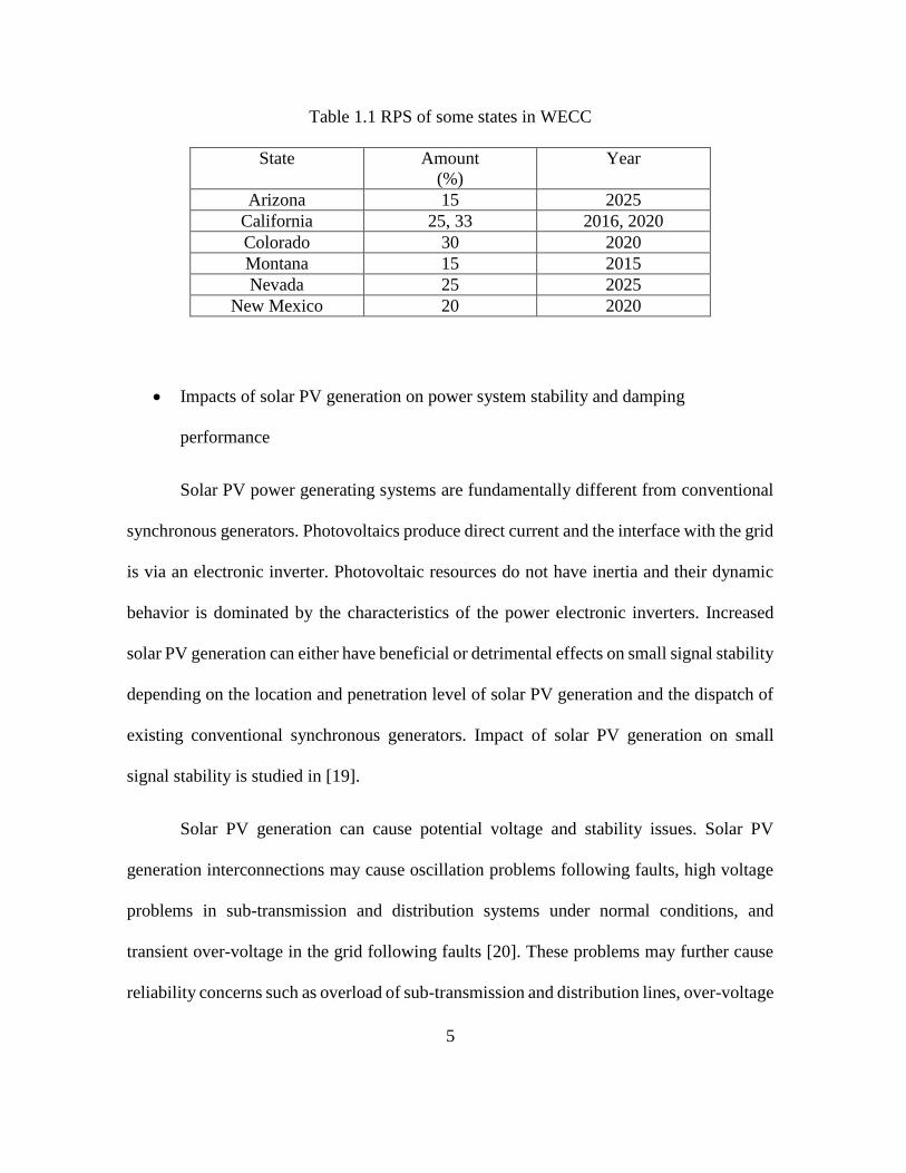
renewable energy sources [18]. The RPS of some of the states in WECC are shown in Table
1.1.
5
Table 1.1 RPS of some states in WECC
State Amount
(%)
Year
Arizona 15 2025
California 25, 33 2016, 2020
Colorado 30 2020
Montana 15 2015
Nevada 25 2025
New Mexico 20 2020
Impacts of solar PV generation on power system stability and damping
performance
Solar PV power generating systems are fundamentally different from conventional
synchronous generators. Photovoltaics produce direct current and the interface with the grid
is via an electronic inverter. Photovoltaic resources do not have inertia and their dynamic
behavior is dominated by the characteristics of the power electronic inverters. Increased
solar PV generation can either have beneficial or detrimental effects on small signal stability
depending on the location and penetration level of solar PV generation and the dispatch of
existing conventional synchronous generators. Impact of solar PV generation on small
signal stability is studied in [19].
Solar PV generation can cause potential voltage and stability issues. Solar PV
generation interconnections may cause oscillation problems following faults, high voltage
problems in sub-transmission and distribution systems under normal conditions, and
transient over-voltage in the grid following faults [20]. These problems may further cause
reliability concerns such as overload of sub-transmission and distribution lines, over-voltage

6
generation tripping, and transient instability. At low levels of penetration, none of these
issues are present, but at high levels of penetration, there is a reasonable motivation to study
and assess the problematic issues indicated. When oscillation problems arise in the system
due to large solar PV integration, critical synchronous generators need to be kept on-line or
other measures such as SVC or power system stabilizer tuning, need to be taken to maintain
sufficient damping of these low frequency oscillations [19].
Voltage stability studies are carried out using PV curves and small-perturbation
stability studies are performed (based on eigenvalue analyses of linearized system models),
and time-domain studies are carried out to examine the overall performance of the system
in case of contingencies. This is the general approach taken in [21].
1.4 Organization of this thesis
Chapter 1 begins with the scope of the topic of research. It further introduces the
impacts of high solar PV generation on power system stability and damping of low
frequency oscillations. Chapter 2 explains the Larsen and Swann method of PSS tuning.
The advantages of these methods are also discussed along with the reason for not
implementing the Larsen and Swann method of power system stabilizer tuning. Chapter 3
discusses the 2010 spring light load case in details. The base case scenario and the scenarios
with changing PV penetration are analyzed. Varying levels of PV generation are considered.
The impacts on frequency and damping of oscillations are observed. Results obtained by
eigenvalue analysis are verified using time domain simulations. Corrective measures to
improve the damping are implemented. The improvement in damping is observed
graphically. Chapter 4 follows-up on the approach and analysis taken in Chapter 3 except

7
that the 2018 summer peak load data is considered and analyzed. Chapter 5 summarizes the
conclusions and is followed by references.
The tests to shut down conventional generation (Test 1 – Test 3), retune PSS (Test
4) and carry out time domain analysis (Test 5) are given in Appendix A. Appendix B gives
the MATLAB code for the example of PSS design (shown in Chapter 2) using the Larsen
and Swann method of PSS tuning.

8
CHAPTER 2 THE LARSEN AND SWANN METHOD FOR PSS TUNING
2.1 Power system damping and the role of a power system stabilizer
An electrical power system is a network of electrical components used to generate,
transmit, supply and use electric power. For AC power systems, power system stability is
an important operating consideration. The performance of a power transmission system
depends on its various components like generation and excitation units, loads, capacitors
and reactors, power electronic devices, and protective devices [2]. While the system
reliability is high, excitation systems with high gain and low time constants may initiate low
frequency oscillations that may persist for long periods of time and cause limitations in
transmitting power. Power system stabilizers are used to provide damping for these
undesirable oscillations.
The basic function of a PSS is to provide damping to system oscillations via
modulation of generator excitation. The oscillations of concern typically occur in the
frequency range of approximately 0.2 to 2.5 Hz, and insufficient damping of these
oscillations may limit power transfer capability [2]. A PSS takes local inputs (speed,
frequency, voltage, power) and provides an auxiliary signal to damp oscillations. For any
input signal the transfer function of the stabilizer should compensate for the gain and phase
characteristics of the excitation system, the generator and the power system itself. The input
signal determines the transfer function from the control input to the excitation system to the
component of electrical torque which can be modulated via excitation control. The exciter
transfer function is influenced by voltage regulator gain, generator power level and the AC
system itself.

9
2.2 The Larsen and Swann method of PSS tuning
PSS tuning is an important concept. Tuning of PSS consists of obtaining correct
parameters to achieve satisfactory performance of the power system. Tuning of PSS helps
provide an auxiliary signal to damp oscillations. This is done by adjusting the lead/lag
parameters of the PSS depending on the phase lag to be compensated.
The steps involved in the Larsen and Swann method of PSS tuning are discussed
below. Fig. 2.1 shows the simplified model of a single machine connected to an infinite bus
[2]. The tuning procedure consists of the following steps:
1. Calculate the transfer function GEP(s) as shown in Fig. 2.1. [2]
2. Plot the phase lag of GEP(s) over the range of frequency of interest.
3. Tune the PSS as to provide suitable phase lead at this desired frequency.
4. Adjust the gain of the PSS (Ks) to one-third of the value that causes instability.
Note that the generator-exciter system in state space form is given by,
�̇� = 𝐴𝑠𝑦𝑠𝑥 + 𝐵𝑠𝑦𝑠𝑢
𝑦 = 𝐶𝑠𝑦𝑠𝑥 + 𝐷𝑠𝑦𝑠𝑢
𝑦 = [𝐶𝑠𝑦𝑠(𝑠𝐼 − 𝐴𝑠𝑦𝑠)−1
𝐵𝑠𝑦𝑠 + 𝐷𝑠𝑦𝑠] 𝑢
𝐺𝐸𝑃(𝑠) = [𝐶𝑠𝑦𝑠(𝑠𝐼 − 𝐴𝑠𝑦𝑠)−1
𝐵𝑠𝑦𝑠 + 𝐷𝑠𝑦𝑠]
where Asys, Bsys, Csys and Dsys are the system matrices.

10
Fig 2.1 Simplified model of a single machine to an infinite bus
2.3 An example to demonstrate the Larsen and Swann method of PSS tuning
An example of the Larsen and Swann method is shown for reference. This example
is applied to a small system. The dynamics of a simple two area power system shown in Fig
2.2 taken directly from [10] is to be improved. Each generator in the system is modeled with
a fast response AC exciter. It is desired to add a PSS to each generator to improve the
dynamic performance of the system.
The base case power flow solution of the two area system has a tie line power flow
of 300 MW. The tie line power flow is increased by 50% to the steady state stability limit

11
of 376.7 MW, to 338.4 MW. The PSS at each generator is tuned using the Larsen and
Swann method. The gain of all power system stabilizers is the same at all the four generators
and is determined through eigenvalue analysis and time domain simulations.
Fig 2.2 A two-area power system used as a test bed
For the example considered, the generators are modeled as model DG0S5 which
represent the synchronous machine as a solid rotor generator, the exciter is modeled as the
AC exciter (EXC30) [22].
The design steps for PSS design using the Larsen and Swann method are as follows:
1 Obtain System matrices Asys , Bsys , Csys , Dsys from power system simulation tools
like DSA Tools.
2 Remove all the rows and columns due to rotor angles and speed and obtain A’, B’,
C’, D’ matrices.
3 Form the overall system transfer function GEP(s), draw the phase curve of GEP(s)
– the ideal phase lead requirement by the PSS.

12
4 Choose PSS time constants to match the ideal curve over 0.1 to 2 Hz (the frequency
range of interest for small signal stability). The PSS is forced to under compensate
at frequencies below 1 Hz so that it does not reduce the synchronizing torque.
5 PSS gain is set using SSAT (complete eigenvalue analysis) and TSAT (time domain
simulations).
2.3.1 Obtaining system state space representation (Matrices Asys, Bsys, Csys, Dsys)
For each dynamic device, SSAT formulates the following model and uses it in all
computations,
[𝑥�̇� = 𝐴𝑑𝑥𝑑 + 𝐵𝑑𝑣𝑑 + 𝐹𝑑𝑢] (2.1)
[𝑖�̇� = 𝐶𝑑𝑥𝑑 + 𝐷𝑑𝑣𝑑] (2.2)
where xd is the n x 1 state vector for a device, vd is the 2m x 1 voltage vector of voltages at
the device terminal bus and any remote sensing buses, and id is the 2k x 1 currents injected
into the network at the device terminals. If response computation is required and the input
is specified as either Vref in an exciter or Pref in a governor, the input is contained in the
vector u. For the system shown in Fig 2.2, the state variables for each generator-exciter
system is given by the following equation
[𝑥𝑑 = (𝜔, 𝛿, 𝜓𝑓𝑑 , 𝜓𝑘𝑑1, 𝜓𝑘𝑞1, 𝜓𝑘𝑞2, 𝑥𝑇𝐹 , 𝑥𝑇𝐵, 𝑥𝑇𝐴)𝑇
]. (2.3)

13
In DSA Tools, the generator states are placed before the exciter states for each
machine in the vector of states. After running the complete eigenvalue analysis in SSAT,
the overall system state matrix Asys is computed from Ad, Bd, Cd, Dd and Yn as,
[𝐴𝑠𝑦𝑠 = 𝐴𝑑 + 𝐵𝑑(𝑌𝑛 − 𝐷𝑑)−1𝐶𝑑] (2.4)
where,
𝐴𝑑 = [𝐴𝑑1
⋱𝐴𝑑𝑛
] 𝐵𝑑 = [𝐵𝑑1
⋱𝐵𝑑𝑛
]
𝐶𝑑 = [𝐶𝑑1
⋱𝐶𝑑𝑛
] 𝐷𝑑 = [𝐷𝑑1
⋱𝐷𝑑𝑛
]
and Yn is the reduced network admittance matrix.
The complete system can be represented by the linearized set of Equations (2.5, 2.6)
where input u is the exciter Vref and the output y is the electrical torque Te. The system
matrices are obtained from SSAT. The details are as follows,
[�̇� = 𝐴𝑠𝑦𝑠𝑥 + 𝐵𝑠𝑦𝑠𝑢]
(2.5)
[𝑦 = 𝐶𝑠𝑦𝑠𝑥 + 𝐷𝑠𝑦𝑠]. (2.6)
For this system studied, the size of the Asys matrix is 36 × 36; the size of the Bsys matrix is
36 × 4; and the size of the Csys matrix is 4 × 36.

14
2.3.2 Estimation of generator-exciter transfer function
The rows and columns corresponding to the speed and rotor angle equations are
removed from the Asys, Bsys, Csys, Dsys matrices to obtain the new state space representation
A’, B’, C’, D’.
The generator-exciter transfer function is obtained as
[𝐺𝐸𝑃(𝑠) = 𝐶′(𝑠𝐼 − 𝐴′)−1𝐵′]. (2.7)
2.3.3 Obtaining the generator-exciter phase plots for the two-area system in Fig 2.2
The phase angle lag of the generator-exciter system is plotted over the range of 0 to
2 Hz for each generator. The time constants of the PSS are found by curve fitting the PSS
frequency response to the generator-exciter lag characteristic. The curve fitting process is
biased to force the PSS to undercompensate at lower frequencies. The frequency responses
for generators 1, 2, 3, and 4 in the two-area system can be seen in Fig 2.3, 2.4, 2.5, and 2.6
respectively.

15
Fig 2.3 Generator-exciter 1 system frequency-phase plot for the two-area system in Section 2.3
Fig 2.4 Generator-exciter 2 system frequency-phase plot for the two-area system in Section 2.3

16
Fig 2.5 Generator-exciter 3 system frequency-phase plot for the two-area system in Section 2.3
Fig 2.6 Generator-exciter 4 system frequency-phase plot for the two-area system in
Section 2.3
17
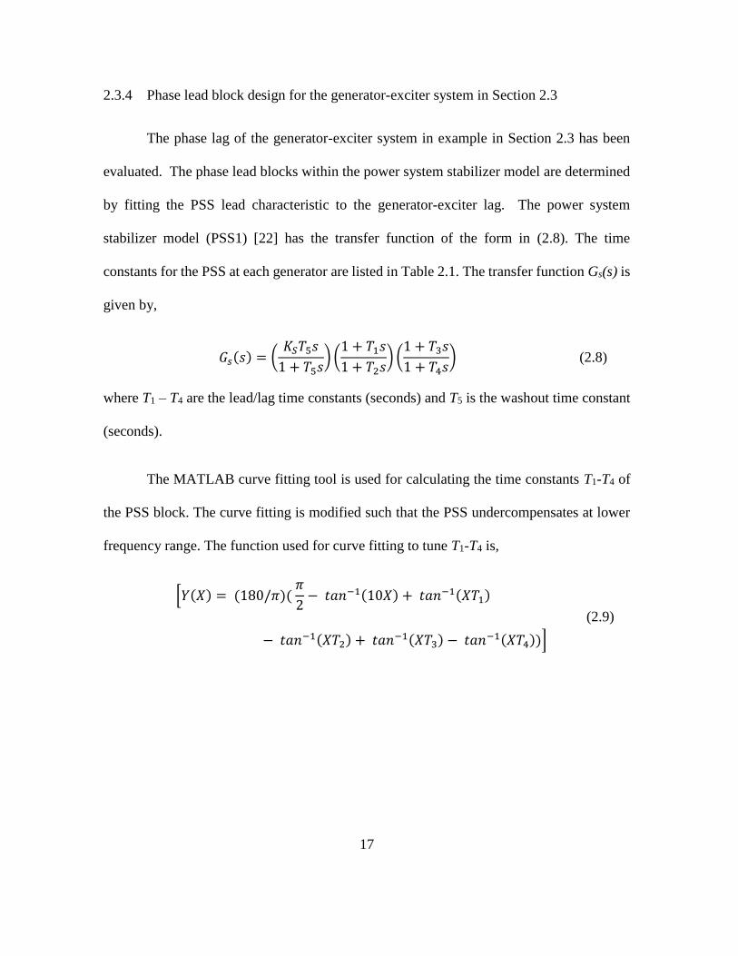
2.3.4 Phase lead block design for the generator-exciter system in Section 2.3
The phase lag of the generator-exciter system in example in Section 2.3 has been
evaluated. The phase lead blocks within the power system stabilizer model are determined
by fitting the PSS lead characteristic to the generator-exciter lag. The power system
stabilizer model (PSS1) [22] has the transfer function of the form in (2.8). The time
constants for the PSS at each generator are listed in Table 2.1. The transfer function Gs(s) is
given by,
𝐺𝑠(𝑠) = (𝐾𝑆𝑇5𝑠
1 + 𝑇5𝑠) (
1 + 𝑇1𝑠
1 + 𝑇2𝑠) (
1 + 𝑇3𝑠
1 + 𝑇4𝑠) (2.8)
where T1 – T4 are the lead/lag time constants (seconds) and T5 is the washout time constant
(seconds).
The MATLAB curve fitting tool is used for calculating the time constants T1-T4 of
the PSS block. The curve fitting is modified such that the PSS undercompensates at lower
frequency range. The function used for curve fitting to tune T1-T4 is,
[𝑌(𝑋) = (180/𝜋)( 𝜋
2− 𝑡𝑎𝑛−1(10𝑋) + 𝑡𝑎𝑛−1(𝑋𝑇1)
− 𝑡𝑎𝑛−1(𝑋𝑇2) + 𝑡𝑎𝑛−1(𝑋𝑇3) − 𝑡𝑎𝑛−1(𝑋𝑇4))]
(2.9)

18
Table 2.1 PSS lead-lag parameters (seconds)
PSS 1 PSS 2 PSS 3 PSS 4
T1 0.9334 0.8919 0.8950 0.8513
T2 0.0100 0.0100 0.0100 0.0100
T3 0.1785 0.1920 0.1817 0.1823
T4 0.0127 0.0100 0.0107 0.0100
T5 10 10 10 10
2.3.5 Select PSS gain using eigenvalue analysis and time domain simulations
All the time constants for the PSS are now defined. The gain of the stabilizers still
needs to be chosen. The gain of all the stabilizers will be held the same. Time domain
simulations of a 6-cycle-duration three-phase fault in the middle of the tie line are conducted
for different PSS gain. A good choice of gain for the stabilizers will provide sufficient
damping torque to each generator in the system. The value of gain Ks is varied from 0 to 15.
For each different gain, an eigenvalue analysis is also conducted to see the effect of the
stabilizers on the critical mode. For PSS gains of 5, the system is underdamped. For gain Ks
of 10 and 11, the system has acceptable overshoot and settling time. For gains of 15 and
above, the system has prolonged overshoot and increased settling time. Table 2.2 shows the
results obtained from eigenvalue analysis for exciter model EXC30.

19
Table 2.2 Results obtained from eigenvalue analysis for the exciter EXC30 in Section 2.3
No.
PSS
Gain
Eigenvalue
Frequency
(Hz)
Damping
(%)
Critical
Mode Real Imaginary
1 No PSS -0.0631 2.3904 0.3804 2.64 Speed
Larsen and Swann Method
2 5.0 -0.3004 2.4513 0.3901 12.16 Speed
3 10.0 -0.5210 2.5020 0.3982 20.38 Speed
4 11.0 -0.5628 2.5103 0.3995 21.88 Speed
5 15.0 -0.7250 2.5385 0.4040 27.46 Speed
6 20.0 -0.9139 2.5607 0.4076 33.61 Speed
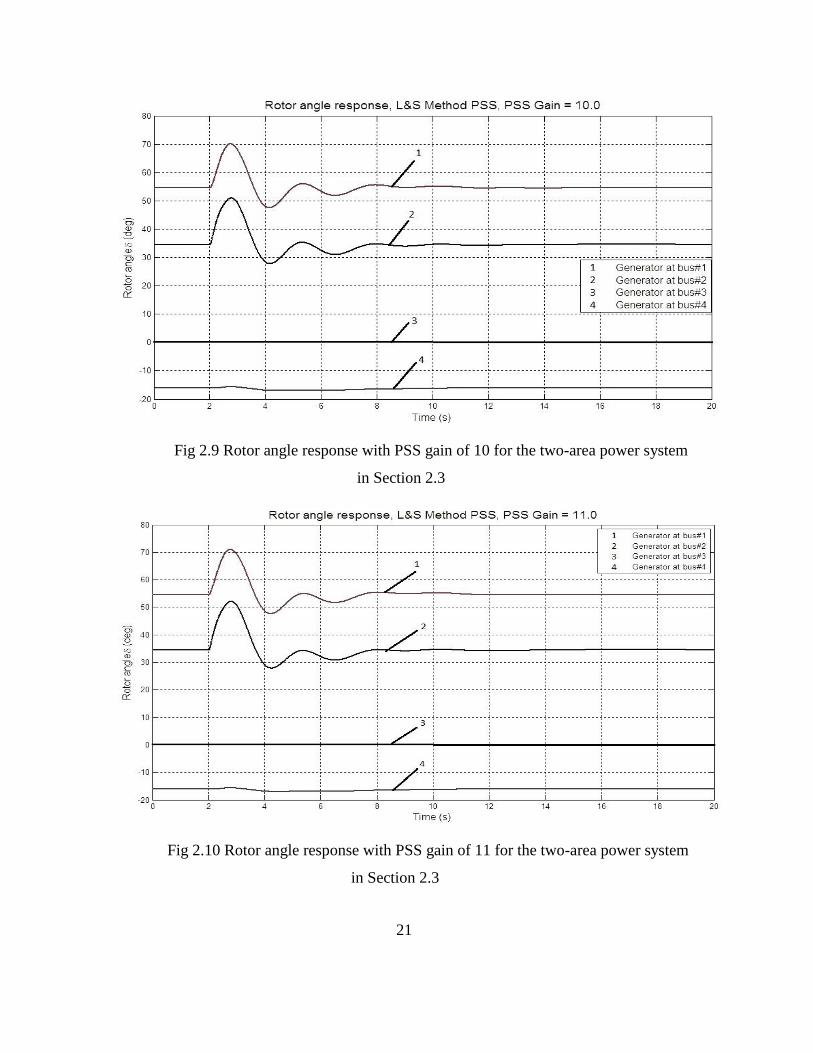
Time domain simulations of the system in the example of Section 2.3 are conducted in
TSAT. The power flow on the tie line in the two-area power system in the example is set to
338.46 MW. A three phase fault was applied at the middle of the tie line with a fixed clearing
time of 6 cycles. The machine rotor angles are plotted for different values of PSS gain. The
results of these simulations can be seen in Fig 2.7 to Fig 2.12. The Larsen and Swann method
of PSS tuning for the two-area system studied in the example is implemented using a code
in Matlab. The code for the same is attached in Appendix B.

20
Fig 2.7 Rotor angle response with no PSS for the two-area power system in
Section 2.3
Fig 2.8 Rotor angle response with PSS Gain of 5.0 for the two-area power system in
Section 2.3
21
Fig 2.9 Rotor angle response with PSS gain of 10 for the two-area power system
in Section 2.3
Fig 2.10 Rotor angle response with PSS gain of 11 for the two-area power system
in Section 2.3

22
Fig 2.11 Rotor angle response with PSS gain of 15 for the two-area power system in Section
2.3
Fig 2.12 Rotor angle response with PSS gain of 20 for the two-area power system in Section
2.3.

23
2.4 Software limitations of the method
The actual power system data used as the test bed for the study is typical of the
analysis data for a large system. Due to the large size of the system at hand and also the
software limitations on the number of states, it is inconvenient to calculate the system
matrices for the entire system. Hence, a method of PSS tuning different from the Larsen
Swan algorithm is implemented. This alternative method is described in Chapter 3.
The SSAT DSA Tool [5] allows for eigenvalue analysis over a selected range of
frequency and damping which gives the matrices for individual units. However, SSAT does
not allow for complete eigenvalue analysis, since the number of states in the system exceeds
the limit set by SSAT. As a result, the system matrices cannot be obtained.

24
CHAPTER 3 EXAMINATION OF OPERATING CONDITIONS WITH INCREASED
SOLAR PENETRATION: SPRING 2010 LIGHT LOAD CASE
3.1 A test bed for an illustrative study
In order to assess the impact of high penetration of PV solar resources, operating
data from the actual power system considered available for the spring 2010 light load case
were used. These data exhibit the aforementioned high level of solar generation. In order to
study this case, a commercial dynamic analysis software package was used to calculate
power system dynamic models. In the study of small-signal power system dynamics, the
time response of rotor angles of generators is characterized by modes. These modes may
be oscillatory or completely damped. The critical modes are those with reduced damping.
Reduced damping is particularly undesirable since the oscillations require longer time to
decay. Such problematic modes are identified. The PSSs on the generators which participate
in these dominant modes are then retuned to account for the changed operating conditions
and improve the damping.
3.2 Description of the test: Spring 2010 light load case
For the spring 2010 light load data, a base case power flow is run and the local and
inter-area modes are observed for frequency and damping. The base case is the case with
zero solar PV generation. As the solar penetration level is added and the PV generation is
increased, the effects on damping show that damping is reduced and modal frequencies are
approximately unchanged. The solar PV penetration is added in steps of 10% up to 50% in
order to assess the impact on system dynamics. The 30%, 40% and 50% penetration levels

25
show significantly lowered damping of the critical modes. In depth analyses of the area, the
type of plant, and the generators are conducted corresponding to the dominant modes.
3.3 Base case scenario: Spring 2010 light load case
The base case (with no PV penetration) is considered and eigenvalue analysis is
carried out using the SSAT DSA tool [5] to check the frequency and damping of the
identified critical modes. These are standard software tools that are widely used in the
electric power industry. For the base case, the eigenvalues associated with the dominant
modes are shown in Table 3.1. Note that damping is represented as a percentage and as a
positive number D.
Table 3.1 Base case dominant modes: Spring 2010 light load case
Mode
number
Eigenvalue
f (Hz)
Damping
D (%)
Dominant
state Real Imaginary
14 -2.4105 20.9021 3.3267 11.46 Angle
15 -2.436 19.7426 3.1421 12.25 Angle
90 -0.908 22.0733 3.5131 4.11 Speed
91 -0.6759 20.4277 3.2512 3.31 Speed
88 -0.7957 18.8228 2.9958 4.22 Speed
88 -1.0736 21.2937 3.389 5.04 Speed
89 -0.8275 19.152 3.0481 4.32 Speed
89 -1.0736 21.2937 3.389 5.04 Speed

26
3.4 Solar PV penetration set at 10% and 20%
The described test bed was also studied with PV generation added. For example,
10% of the total name plate generation was supplied by PV and in turn, some conventional
generators were shut down in order to account for this additional generation. Similar steps
were carried out for the 20% case. The results are produced in Tables 3.2 and 3.3.
It is observed that the 10% and 20% PV generation cases did not impact damping.
Hence these cases are not considered for further analysis. Different scenarios were then
studied where specific generators were switched off to allow for the high PV generation.
Table 3.2 Dominant modes for the 10% PV generation case: Spring 2010 light load case
Mode
number
Eigenvalue
f (Hz)
Damping
D (%)
Dominant
state Real Imaginary
14 -2.4027 20.8901 3.3248 11.43 Angle
15 -2.4204 19.7196 3.1385 12.18 Angle
91 -0.7527 21.2089 3.3755 3.55 Speed
88 -0.8806 18.488 2.9425 4.76 Angle
88 -1.1691 20.7993 3.3103 5.61 Speed
89 -0.9133 18.7964 2.9916 4.85 Speed
89 -1.1691 20.7993 3.3103 5.61 Angle

27
Table 3.3 Dominant modes for the 20% PV generation case: Spring 2010 light load
case
Mode
Number
Eigenvalue f
(Hz)
Damping D
(%)
Dominant
State Real Imaginary
14 -2.3676 19.8119 3.1532 11.87 Angle
88 -0.9353 18.2836 2.9099 5.11 Angle
88 -1.2322 20.509 3.2641 6 Speed
89 -0.97 18.5842 2.9578 5.21 Speed
89 -1.2322 20.509 3.2641 6 Speed
3.5 Generators shut down to allow for the excess PV penetration
As PV generation is added and increased from 30% to 50%, conventional generators
are shut down to allow for the PV generation. The generators shut down for this task were
decided depending on the type of generating units and the amount of generation.
3.5.1 Shutting down the CT and GT units to accommodate PV generation
A test was done to evaluate the reduction of combustion turbine (CT) and gas turbine
(GT) generation. This task deals with altering the economic generation scheduling. Since
the GT and CT units have relatively high operating costs, these types of conventional
generator units are shut down to account for the additional PV generation. The PV is added
in varying amounts (30%, 40%, and 50%) and equal amounts of generation are backed off

28
from conventional generators. The generators that are selected to be shut down belong to
the CT and GT type. The results are shown in Table 3.4.
3.5.2 Shutting down an aging coal unit
In simulation, the generating units at an aging coal generation station are shut down
in order to account for the additional PV generation. The results are shown in Table 3.5.
3.5.3 Shutting down alternative aging coal units
Alternative aging coal units in the area under study are shut down in simulation in
order to account for the additional PV generation. The results are shown in Table 3.6.

29
Table 3.4 Comparison between 30%, 40% and 50% PV penetration cases when CT and
GT units are switched off: Spring 2010 light load case
Dominant
state
Base case 30% PV 40% PV 50% PV
Bus f
(Hz)
D
(%)
f
(Hz)
D
(%)
f
(Hz)
D
(%)
f
(Hz)
D
(%)
14 3.33 11.46 3.32 11.38 3.32 11.43 3.32 11..42
15 3.14 12.25 3.12 12.18 3.12 12.22 3.12 12.23
90 3.51 4.11 3.51 4.12 3.51 4.43 3.50 4.45
91 3.25 3.31 3.26 3.31 3.24 3.34 3.51 2.61
88 3.04 4.32 2.91 5.01 2.98 4.3 3.00 4
88 3.39 5.04 3.27 5.9 3.36 5.15 3.41 4.84
89 2.99 4.22 2.96 5.12 3.03 4.42 3.06 4.13
89 3.39 5.04 3.27 5.9 3.36 5.15 3.41 4.84
Table 3.5 Comparison between 30%, 40% and 50% PV cases when aging coal units are
switched off: Spring 2010 light load case
Dominant
state
Base case 30% PV 40% PV 50% PV
Bus f
(Hz)
D
(%)
f
(Hz)
D
(%)
f
(Hz)
D
(%)
f
(Hz)
D
(%)
88 2.99 4.22 2.91 5.09 2.97 4.4 3.01 4
88 3.39 5.04 3.27 5.98 3.36 5.25 3.41 4.83
89 3.05 4.32 2.96 5.19 3.03 4.51 3.06 4.13
89 3.9 5.04 3.27 5.98 3.36 5.25 3.41 4.83

30
Table 3.6 Comparison between 30%, 40% and 50% PV cases when alternative aging coal
units are switched off: Spring 2010 light load case
Dominant state Base case 30% PV 40% PV 50% PV
Bus F
(Hz)
D
(%)
f
(Hz)
D
(%)
f
(Hz)
D
(%)
f
(Hz)
D
(%)
90 3.51 4.11 3.55 4.04 3.51 4.35 3.50 4.49
91 3.25 3.31 3.25 3.25 3.24 3.3 3.19 2.8
88 2.99 4.22 2.90 5.2 2.96 4.48 3.01 3.99
88 3.39 5.04 3.25 6.1 3.34 5.34 3.41 4.83
89 3.05 4.32 2.95 5.31 3.02 4.6 3.07 4.12
89 3.39 5.04 3.25 6.1 3.35 5.34 3.42 4.83
3.6 Time domain analysis
The 50% PV penetration case with the CT and GT units turned off (Table 3.4) shows
the lowest damping for the dominant mode at a specific system generation bus 91. This case
is considered for further analysis. Time domain analysis is conducted using the TSAT. A
three-phase fault is created on the bus which is electrically closest to bus 91 since such a
fault affects the critically damped modes the most. The fault is cleared after 6 cycles. The
behavior of the generator at bus 91 is monitored and generator speed is plotted in Fig. 3.1.
Further, Prony analysis is conducted to validate the results and the dominant modes are
shown in Table 3.7.
3.7 Prony analysis
Prony analysis is a feature of the TSAT DSA tool and is used in time-domain
simulations. Prony analysis is a methodology that extends Fourier analysis by directly

31
estimating the frequency, damping strength and relative phase of the modal components
present in a given signal [12]. The ability to extract such information from transient stability
program simulations and from large scale system tests or disturbances could provide:
Parametric summaries for damping studies (data compression)
Quantified information for adjusting remedial controls (sensitivity analysis and
performance evaluation)
Insight into modal interaction mechanisms (modal analysis)
Reduced simulation times for damping evaluation (prediction).
A linear, time-invariant dynamic system is brought to an initial state x(t0) = x0 at
time t0. This is done by introducing a test input or disturbance. If the input is removed
without any subsequent inputs or disturbances, the system state will ‘ring down’ according
to a linearized differential equation of the form
ẋ = Ax
where x is the state of the system and n is the order of the system. The solution to the above
equation is expressed in terms of the eigenvalues, right eigenvectors and left eigenvectors
of matrix A.
The strategy for obtaining Prony solution is summarized as follows:
1. Construct a discrete linear prediction model that fits the record.
2. Find the roots of the characteristic polynomial associated with the linear prediction
model.

32
3. Using the roots as the complex modal frequencies for the signal, determine the
amplitude and initial phase for each mode.
These steps are performed in z-domain. For power system application, the eigenvalues
would be translated to s-domain. Prony’s main contribution is at step 1.
Fig 3.1 Generator 91 speed plot with the original PSS settings: Spring 2010 light load case
The time domain simulation are carried out as defined in test 5 (Appendix A) and
the results are shown in Table 3.7 identify the poorly damped mode of oscillation (mode 6).
This result is consistent with the result produced in Table 3.4 that identifies the mode
associated with the dominant state at generation bus 91. The critical mode has a frequency
of 3.51 Hz and damping of 2.61%.

33
Table 3.7 Time domain results: Spring 2010 light load case
Mode number f (Hz) D (%)
1 21.684 41.954
2 13.238 52.599
3 30.25 33.573
4 2.97 14.357
5 1.213 69.4
6 3.342 2.868
7 9.00 16.784
3.8 Power system stabilizer tuning
Due to the limitations in the implementation of the Larsen and Swann method for
PSS tuning, this method cannot be used to retune the PSSs existing on the identified
conventional generators. Another method of PSS retuning is adopted. The modes
corresponding to buses 90 and 91 have to be retuned simultaneously since retuning the mode
with the critically low damping caused the damping of the other mode to reduce. This
method is based on the procedure described in reference [9]. The steps involved are as
below,
1. Using SSAT, the frequency response of the transfer function for the dominant mode
at bus 91 without the PSS is plotted in Fig 3.2. This was done because the system
size does not allow the direct calculation of the system matrices.
2. At the frequency of the mode at 3.51 Hz, the corresponding phase lag of 136.4
degrees is obtained.

34
3. The data from the SSAT is used to plot the frequency response in MATLAB.
4. For the above phase lag, the lead / lag time constants T1, T2, T3, T4 are calculated
using a MATLAB code for PSS design using,
𝑓 = 3.51
𝜔 = 2𝜋 𝑓
𝜃 = −136.4𝜋
180 × 2
𝛼 = (1 + sin 𝜃)
(1 − sin 𝜃)
𝜏 = 1
𝜔√𝛼
with α and τ being the lead / lag time constants, and these expressions are in Hz, r/s, radians
and seconds.
5. Similar steps were carried out for the dominant mode at bus 90 for a phase lag of
96.5 degrees.
Fig 3.2 Frequency response of the 91 generator-exciter transfer function: Spring 2010 light
load case

35
3.9 Results of PSS retuning
After the retuning process, the new values of time constants obtained are then fed
into the dynamic data file in SSAT. The time constants before and after retuning are shown
in Table 3.8.
Table 3.8 Original and new values of PSS lead/lag time constants: Spring 2010 light load
case
Dominant
generator
modes
T1 T2 T3 T4
(seconds)
90 0.6 0.07 0.6 0.07
91 0.6 0.07 0.6 0.07
New values for PSS retuning
90 0.0371 0.2358 0.0371 0.2358
91 0.1454 0.1191 0.1454 0.1191
The T1-T4 time constants for the standard IEEE- PSS model [11] were modified in
the retuned PSS and the eigenvalue analysis is once again carried out using SSAT. The new
results were compared with the original results and are shown in Table 3.9.
Table 3.9 Improvement in damping of the identified modes on retuning the PSS: spring
2010 light load case
Dominant
generator
modes
50% PV case
Original PSS settings Retuned PSS
f (Hz) D (%) f (Hz) D (%)
90 3.50 4.45 3.4121 7.38
91 3.51 2.61 3.1179 5.90
36
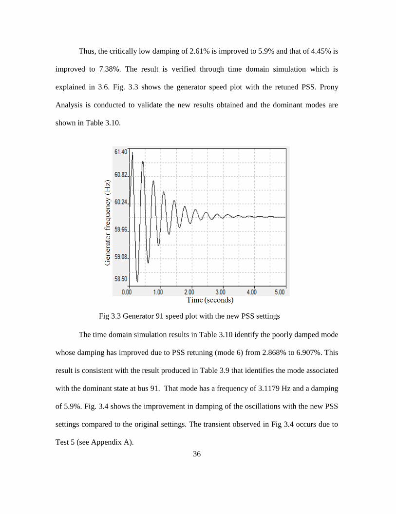
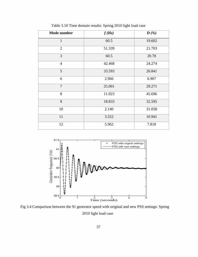
Thus, the critically low damping of 2.61% is improved to 5.9% and that of 4.45% is
improved to 7.38%. The result is verified through time domain simulation which is
explained in 3.6. Fig. 3.3 shows the generator speed plot with the retuned PSS. Prony
Analysis is conducted to validate the new results obtained and the dominant modes are
shown in Table 3.10.
Fig 3.3 Generator 91 speed plot with the new PSS settings
The time domain simulation results in Table 3.10 identify the poorly damped mode
whose damping has improved due to PSS retuning (mode 6) from 2.868% to 6.907%. This
result is consistent with the result produced in Table 3.9 that identifies the mode associated
with the dominant state at bus 91. That mode has a frequency of 3.1179 Hz and a damping
of 5.9%. Fig. 3.4 shows the improvement in damping of the oscillations with the new PSS
settings compared to the original settings. The transient observed in Fig 3.4 occurs due to
Test 5 (see Appendix A).
37
Table 3.10 Time domain results: Spring 2010 light load case
Mode number f (Hz) D (%)
1 60.5 19.602
2 51.339 21.703
3 60.5 20.78
4 42.468 24.274
5 33.593 26.841
6 2.966 6.907
7 25.001 29.271
8 11.923 45.696
9 18.833 32.595
10 2.140 31.058
11 3.552 10.941
12 5.962 7.818
Fig 3.4 Comparison between the 91 generator speed with original and new PSS settings: Spring
2010 light load case

38
The impact of PV penetration on selected buses is observed. Eigenvalue analysis is
carried out and reduction in damping performance is observed. Time domain simulations
(test 5 – Appendix A) are also performed to see the oscillations which take longer time to
damp. The PSS existing on the generators observed are retuned to damp the oscillations
faster. The improvement in damping is observed graphically as the generator speed is
plotted for the case where the PSS is at the original setting and the case where the PSS is
retuned.
39
CHAPTER 4 EXAMINATION OF OPERATING CONDITIONS WITH INCREASED
SOLAR PENETRATION: SUMMER 2018 PEAK LOAD CASE
4.1 A test bed for an illustrative study
In order to assess the impact of high penetration of PV solar resources, operating
data from the actual power system considered for the summer 2018 peak load case were
used. These data exhibit the aforementioned high level of solar generation. In order to study
this case, the commercial dynamic software package used to study summer 2018 peak load
data was used to calculate power system dynamic models. In the study of small-signal power
system dynamics, the time response of rotor angles of generators, characterized by modes,
may be oscillatory or completely damped. The critical modes are those with reduced
damping. Reduced damping is particularly undesirable since the oscillations require longer
time to decay. Such problematic modes are identified. The PSSs on the generators which
participate in these dominant modes are then retuned to account for the changed operating
conditions and improve the damping.
4.2 Description of the test: Summer 2018 peak load case
For the summer 2018 peak load data, a base case power flow is run and the local and
inter-area modes are observed for frequency and damping. The base has zero solar PV
generation. As the solar penetration level is added and the PV generation is increased, the
effects on damping show that damping is reduced and modal frequencies are approximately
unchanged. The solar PV penetration is added in steps of 10% up to 50% in order to assess
the impact on system dynamics. The damping of the critical modes is lowered as the

40
penetration of PV generation is increased up to 50%. In depth analyses of the area, the type
of plant, and the generators are conducted corresponding to the dominant modes.
4.3 Base case scenario: Summer 2018 peak load case
The steps followed are similar to the steps followed for the assessment of the spring
light load case. The base case (with zero PV penetration) is considered and eigenvalue
analysis is carried out using the SSAT DSA tool to check the frequency and damping of the
identified critical modes. For the base case, the eigenvalues associated with the dominant
modes are shown in Table 4.1. Damping is represented as a percentage and as a positive
number D.
Table 4.1 Base case dominant modes: Summer 2018 peak load case
Mode
number
Eigenvalue
f (Hz)
Damping
D (%)
Dominant
state Real Imaginary
93 -0.7971 18.7865 3.0754 1.81 Speed
94 -1.5115 20.8487 3.4336 3.65 Speed
95 -1.0169 18.4465 3.0625 2.37 Speed
96 -1.4946 20.7996 3.4107 4.42 Angle
97 -0.997 18.4594 3.0477 2.85 Speed
98 -1.4801 20.8878 3.4424 3.46 Speed
99 -1.5224 18.2267 3.0699 2.03 Speed

41
4.4 Generators shut down to allow for the excess PV penetration
As PV generation is added and increased from 10% to 50%, conventional generators
are shut down to allow for the PV generation. The generators shut down for this task were
decided depending on the type of generating units and the amount of generation.
Shutting down the CT and GT units
This is carried out on the steps of Test 1 (see Appendix A). The PV is added in
increasing amounts (10%, 20%, 30%, 40% and 50%) and equal amounts of generation are
backed off from conventional generators. The generators that are selected to be shut down
belong to the CT and GT type. The results are shown in Table 4.2.
Table 4.2 Comparison between 10%, 20%, 30%, 40% and 50% PV penetration cases
when CT and GT units are switched off (test 1)
Dominant
state
Base case 10% 20% 30% 40% 50%
Bus f
(Hz)
D
(%)
f
(Hz)
D
(%)
f
(Hz)
D
(%)
f
(Hz)
D
(%)
f
(Hz)
D
(%)
f
(Hz)
D
(%)
93 3.08 1.81 3.08 1.78 3.08 1.73 3.09 1.65 3.09 1.59 3.09 1.58
94 3.43 3.65 3.44 3.61 3.44 3.54 3.44 3.42 3.44 3.33 3.44 3.32
95 3.06 2.37 3.06 2.34 3.07 2.28 3.07 2.19 3.08 2.13 3.08 2.11
96 3.41 4.42 3.41 4.37 3.41 4.3 3.42 4.17 3.42 4.07 3.42 4.05
97 3.05 2.85 3.05 2.82 3.05 2.76 3.06 2.67 3.06 2.59 3.06 2.58
98 3.44 3.46 3.44 3.42 3.45 3.35 3.45 3.23 3.45 3.14 3.45 3.12

42
From Table 4.2 it is observed that the damping consistently decreases as the PV
generation is increased. Carrying out Tests 1, 2 and 3 (see Appendix A) showed the same
results as obtained in Table 4.2.
4.5 Time domain analysis
The varying PV penetration cases with the CT and GT units turned off (Table 4.2)
show the lowering of damping for the dominant modes at specific system generation buses.
Buses 93 to 98 showed critically low damping as the PV generation was increased. These
cases are considered for further analysis. Time domain analysis is conducted using the
TSAT (see Appendix A for test 5). A three-phase fault is created on bus which is electrically
closest to the identified buses since such a fault affects the critically damped modes the
most. The fault is cleared after 6 cycles. The behavior of the generators at these buses is
monitored and Prony analysis is conducted to validate the results and the dominant modes
are shown in Tables 4.3 - 4.7.
Table 4.3 Time domain results for 10% PV penetration case: Summer 2018 peak load case
Mode number f (Hz) D (%)
1 3.03 3.96
2 3.44 4.61
3 3.01 3.566
4 3.4 5.243
5 3.09 3.687
6 3.48 2.374

43
Table 4.4 Time domain results for 20% PV penetration case: Summer 2018 peak load case
Mode number f (Hz) D (%)
1 3.03 4.517
2 3.44 3.549
3 3.02 3.616
4 3.37 6.25
5 3.08 3.257
6 3.47 4.145
Table 4.5 Time domain results for 30% PV penetration case: Summer 2018 peak load case
Mode number f (Hz) D (%)
1 3.03 3.88
2 3.42 6.82
3 2.88 3.572
4 3.35 6.737
5 3.12 4.012
6 3.47 3.909

44
Table 4.6 Time domain results for 40% PV penetration case: Summer 2018 peak load case
Mode number f (Hz) D (%)
1 2.92 1.017
2 3.52 4.83
3 2.73 1.808
4 3.47 4.145
5 3.09 4.043
6 3.51 5.623
Table 4.7 Time domain results for 50% PV penetration case: Summer 2018 peak load case
Mode number f (Hz) D (%)
1 3.19 4.414
2 3.45 3.31
3 3.26 3.341
4 3.38 4.998
5 3.18 1.444
6 3.49 4.248
The Prony analysis results demonstrate the same trend with the reduction of the
damping as shown by the eigenvalue analysis results
4.6 Steps carried out in retuning the PSS
Task 4 gives the steps to obtain the lead / lag time constants of each power system
stabilizer depending on the phase lag to be compensated by the PSS (see Appendix A). For

45
frequency of each mode, corresponding phase lag was obtained from frequency response of
the excitation system transfer function. Table 4.8 shows the original and the new values of
time constants obtained. Using these new values, the PSS were retuned and improvement
in damping performance is shown in Table 4.9.
Table 4.8 Original and new values of PSS lead/lag time constants: Summer 2018 peak
load case
Dominant
generator modes
T1 T2 T3 T4
(seconds)
93 0.6 0.07 0.6 0.07
94 0.6 0.07 0.6 0.07
95 0.6 0.07 0.6 0.07
96 0.6 0.07 0.6 0.07
97 0.6 0.07 0.6 0.07
98 0.6 0.07 0.6 0.07
New values for PSS retuning
93 0.1249 0.1457 0.1249 0.1457
94 0.0278 0.2770 0.0278 0.2770
95 0.1124 0.1539 0.1124 0.1539
96 0.3739 0.0936 0.3739 0.0936
97 0.1324 0.1428 0.1324 0.1428
98 0.0266 0.2824 0.0266 0.2824
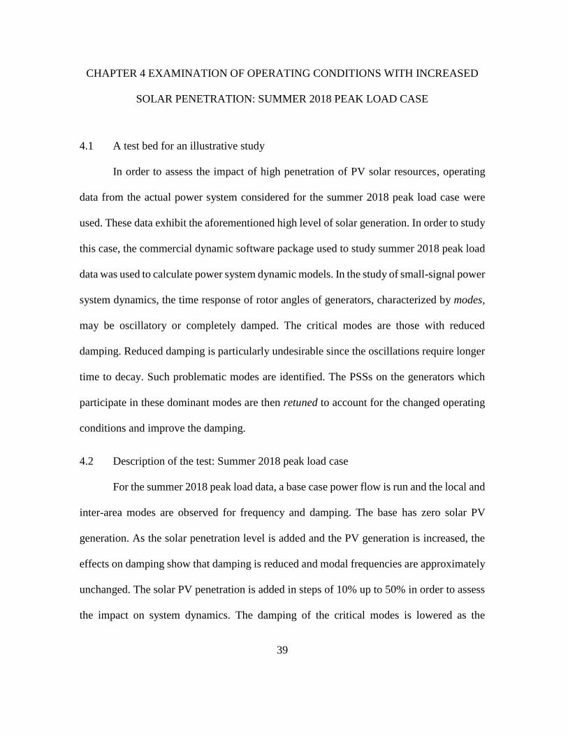
The improvement in damping of the oscillations for the dominant modes at
generators 93 to 98 is observed in TSAT. The damping of oscillations for these modes with
original PSS settings and new PSS settings are plotted and compared. Figures 4.1 – 4.6 show
46
the improvement in the damping performance for these modes (93 – 98) after retuning each
PSS.
Table 4.9 Improvement in damping of the identified modes on retuning the PSS: Summer
2018 peak load case
Dominant
state
Base case 10% 20% 30% 40% 50%
Bus f
(Hz)
D
(%)
f
(Hz)
D
(%)
f
(Hz)
D
(%)
f
(Hz)
D
(%)
f
(Hz)
D
(%)
f
(Hz)
D
(%)
93 3.08 1.81 2.99 4.24 2.9929 4.22 2.9979 4.19 3.002 4.16 3.002 4.16
94 3.43 3.65 3.318 7.23 3.3191 7.2 3.321 7.16 3.323 7.12 3.323 7.11
95 3.06 2.37 2.936 5.5 2.938 5.49 2.943 5.46 2.946 5.44 2.946 5.44
96 3.41 4.42 3.31 7.17 3.311 7.13 3.314 7.07 3.315 7.01 3.316 7.00
97 3.05 2.85 2.938 5.39 2.94 5.38 2.945 5.34 2.948 5.32 2.948 5.31
98 3.44 3.46 3.324 7.07 3.325 7.04 3.327 6.99 3.329 6.95 3.329 6.94
Fig 4.1 Comparison between the 93 generator speed with original and new PSS settings:
Summer 2018 peak load case
47
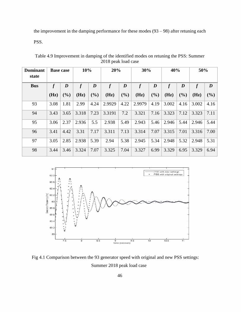
Fig 4.2 Comparison between the 94 generator speed with original and new PSS settings:
Summer 2018 peak load case
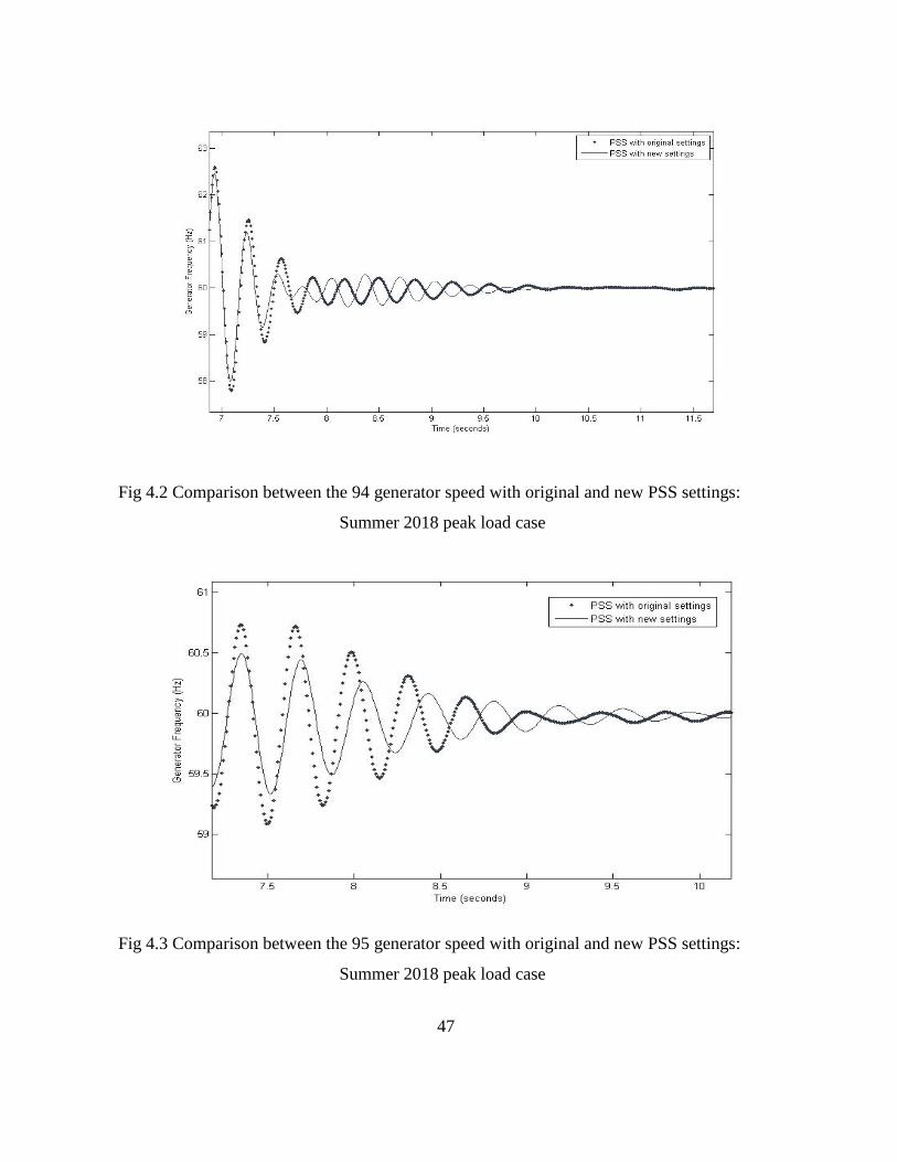
Fig 4.3 Comparison between the 95 generator speed with original and new PSS settings:
Summer 2018 peak load case

48
Fig 4.4 Comparison between the 96 generator speed with original and new PSS settings:
Summer 2018 peak load case
Fig 4.5 Comparison between the 97 generator speed with original and new PSS settings:
Summer 2018 peak load case

49
Fig 4.6 Comparison between the 98 generator speed with original and new PSS settings:
Summer 2018 peak load case
The impact of PV penetration on selected buses (93 - 98) is observed. Eigenvalue
analysis is carried out and reduction in damping performance is observed. Time domain
simulations (test 5 – Appendix A) are also performed to see the oscillations which take
longer time to damp. The PSS existing on the generators observed are retuned to damp the
oscillations faster. The improvement in damping is observed graphically as the generator
speed is plotted for the case where the PSS is at the original setting and the case where the
PSS is retuned.
50
CHAPTER 5 CONCLUSIONS AND RECOMMENDATIONS FOR FUTURE WORK
5.1 Summative remarks
This thesis relates to photovoltaic generation in the electric power system under
study. The impact of solar generation integration on power system dynamics is studied and
evaluated. High photovoltaic solar penetration results in potentially problematic low system
damping operating conditions. This is the case because the power system damping provided
by conventional generation may be insufficient due to:
Reduced system inertia
Change in power flow patterns affecting synchronizing capability in the AC system
This occurs because conventional generators are rescheduled or shut down to allow for
the increased solar production. The effects of high solar PV generation are observed using
eigenvalue analysis and time domain simulations.
5.2 Conclusions
Spring 2010 light load case:
The eigenvalue analysis (Table 3.4) shows poorly damped modes in the system with
high levels of PV generation and the damping worsens as the PV generation
increases. For the spring 2010 light load case, the dominant mode associated with
bus 91 is the critically damped mode and the 50% PV generation case shows it’s
damping as low as 2.61% (Table 3.4).
Prony analysis (time domain) identifies the poorly damped mode as mode 6 (Table
3.7).

51
On retuning, the PSS existing on the generator at bus 91, the damping is improved
and is seen graphically in Fig 3.4.
Summer 2018 peak load case:
The eigenvalue analysis (Table 4.2) shows the poorly damped modes in the system
with high levels of PV generation and the damping worsens as the PV generation
increases. For the summer 2018 peak load case, the dominant mode associated with
buses 93 to 98 show the critically damped modes (Table 4.2).
Prony analysis (time domain) identifies the poorly damped modes (Tables 4.3 – 4.7)
which correspond to the modes in Table 4.2.
On retuning the PSSs existing on generator at bus 94, the damping is improved and
is seen graphically in Fig 4.1. (Similar graphs are generated for other buses in the
summer case and the improvement in damping is observed).
5.3 Recommendations for future work
Future work may involve the following:
Steps to change the PSS settings as obtained after retuning the PSSs on the
generators should be enumerated and identified.
The spring light load data and summer peak load data (data of recent years for the
spring case) should be updated.
The impact of PV generation on buses outside of Arizona should be analyzed. And
the effect of a change in PSS settings on system damping should be evaluated.

52
REFERENCES
[1] S. Eftekharnejad, V. Vittal, G. T. Heydt, B. Keel, J. Loehr, “Impact of Increased
Penetration of Photovoltaic Generation on Power Systems,” To appear in the IEEE
Transactions on Power Systems, 2014.
[2] E. V. Larsen and D. A. Swann, “Applying Power System Stabilizers – Part I: General
Concepts,” IEEE Transactions on Power Apparatus and Systems, vol. PAS-100, No. 6, pp.
3017-3024, June 1981.
[3] E. V. Larsen and D. A. Swann, “Applying Power System Stabilizers – Part II:
Performance Objectives and Tuning Concepts,” IEEE Transactions on Power Apparatus
and Systems, vol. PAS-100, No. 6, pp. 3025-3033, June 1981.
[4] E. V. Larsen and D. A. Swann, “Applying Power System Stabilizers – Part III: Practical
Considerations,” IEEE Transactions on Power Apparatus and Systems, vol. PAS-100, No.
6, pp. 3034-3046, June 1981.
[5] SSAT version 12.0 User’s Manual, Powertech Labs, Inc., April 2012.
[6] TSAT version 12.0 User’s Manual, Powertech Labs, Inc., April 2012.
[7] J. C. H. Peng, N. K. C. Nair, A. L. Maryani, A. Ahmad, “Adaptive Power System
Stabilizer Tuning Technique for Damping Inter-Area Oscillations,” Proceedings of the
IEEE Power and Energy Society General Meeting, July 2010.
[8] O. Abedinia, M. S. Naderi, A. Jalili, B. Khamenehpour, “Optimal Tuning of Multi-
machine Power System Stabilizer Parameters Using Genetic Algorithm,” International
Conference on Power System Technology (POWERCON), October 2010.
[9] P. M. Anderson and A. A. Fouad, Power System Control and Stability, Institute of
Electrical and Electronics Engineers, Inc., 2003.
[10] P. Kundur, Power System Stability and Control, McGraw-Hill, New York, 1994.
[11] PSLF version 18.1_01 User’s Manual, General Electric International, Inc., October
2012.
[12] J. F. Hauer, C. J. Demeure, L. L. Scharf, “Initial Results in Prony Analysis of Power
System Response Signals,” IEEE Transactions on Power Systems, vol. 5, No. 1, February
1990.
[13] Liu Weiping, Lin Miaoshan, “Research and Application of High Concentrating Solar
Photovoltaic System,” IEEE Second International Conference on Consumer Electronics,
Communications and Networks (CECNet), April 2012.

53
[14] C. T. Hsu, L. J. Tsai, T. J. Cheng, C. S. Chen, “Solar PV Generation System Controls
for Improving Voltage in Distribution Network,” IEEE Second International Symposium on
Next-Generation Electronics (ISNE), February 2013.
[15] Shuhui Li, Huiying Zheng, “Energy Extraction Characteristic Study of Solar
Photovoltaic Cells and Modules,” Power and Energy Society General Meeting, IEEE
Publications, July 2011.
[16] C. Hanley, G. Peek, J. Boyes, G. Klise, J. Stein, D. Ton, Tien Duong, “Technology
Development Needs for integrated Grid-connected PV Systems and Electric Energy
Storage,” Photovoltaic Specialists Conference, IEEE Publications, Piscataway NJ, June
2009.
[17] P. M. Jansson, R. A. Michelfelder, V. E. Udo, G. Sheehan, S. Hetznecker, M. Freeman,
“Integrating Large-Scale Photovoltaic Power Plants into the Grid,” Energy 2030
Conference, IEEE Publications, November 2008.
[18] Anonymous, “Renewable Portfolio Standards,” Wikipedia.
http://en.wikipedia.org/w/index.php?title=Renewable_portfolio_standard&oldid=6070982
87
[19] Liu Haifeng, Jin Licheng, D. Le, A. A. Chowdhury, “Impact of High Penetration of
Solar Photovoltaic Generation on Power System Small Signal Stability,” International
Conference on Power System Technology, IEEE Publications, October 2010.
[20] Yi Zhang, Zhu Songzhe, R. Sparks, I. Green, “Impacts of Solar PV Generators on
Power System Stability and Voltage Performance,” IEEE Power and Energy Society
General Meeting, July 2012.
[21] B. Tamimi, C. Canizares, K. Bhattacharya, “Modeling and Performance Analysis of
Large Solar Photovoltaic Generation on Voltage Stability and Inter-area Oscillations,” IEEE
Power and Energy Society General Meeting, July 2011.
[22] DSA Tools TSAT Model Manual, Powertech Labs Inc., March 2013.
[23] A. Pethe, V. Vittal, G. T. Heydt, “Evaluation and Mitigation of Oscillations Arising
from High Solar Penetration due to Low Conventional Generation,” Proc. North American
Power Symposium, Pullman, WA, September 2014.

54
APPENDIX A
TASKS CARRIED OUT FOR SHUTTING DOWN GENERATORS

55
Test 1: Shutting down the CT and GT units to accommodate PV generation
A test was done to evaluate the reduction of combustion turbine (CT) and gas turbine
(GT) generation. This task deals with altering the economic generation scheduling. Since
the GT and CT units have relatively high operating costs, these types of conventional
generator units are shut down to account for the additional PV generation. The PV is added
in varying amounts (30%, 40%, and 50%) and equal amounts of generation are backed off
from conventional generators. The generators that are selected to be shut down belong to
the CT and GT type.
Test 2: Shutting down an aging coal unit
The generating units at an aging coal generation station are shut down in order to
account for the additional PV generation. The units are shut down taking into consideration
their location, participation factor and the type of plant.
Test 3: Shutting down alternative aging coal units
Alternative aging coal units in the area under study are shut down in order to account
for the additional PV generation. The units are shut down taking into consideration their
location, participation factor and the type of plant.
Test 4: Steps carried out for PSS tuning for the summer 2018 peak load case
Using SSAT, the frequency response of the transfer function for the dominant mode
at buses 93 to 98 without the PSS is plotted.

56
At the frequencies of the respective mode, the corresponding phase lags are
obtained.
For the obtained phase lags, the lead / lag time constants T1, T2, T3, T4 are calculated
using a MATLAB code for PSS design shown below:
𝑓 = 𝑓𝑟𝑒𝑞𝑢𝑒𝑛𝑐𝑦 𝑜𝑓 𝑚𝑜𝑑𝑒
𝜔 = 2𝜋 𝑓
𝜃 = −(𝑝ℎ𝑎𝑠𝑒 𝑙𝑎𝑔)𝜋
180 × 2
𝛼 = (1 + sin 𝜃)
(1 − sin 𝜃)
𝜏 = 1
𝜔√𝛼
with α and τ being the lead / lag time constants, and these expressions are in Hz, r/s, degrees
and seconds.
Test 5: Time domain analysis
Time domain analysis is conducted using the TSAT. A three-phase fault is created
on the bus which is electrically closest to bus whose behavior is observed since such a fault
affects the critically damped modes the most. The fault is cleared after 6 cycles. The
behavior of the generator at the selected bus is monitored.

57
APPENDIX B
MATLAB CODE FOR PSS TUNING – LARSEN AND SWANN METHOD

58
%%%%%%%%%%%%%%%%%%%%%%%%%%%%%%%%%%%%%%%%%%%
%%%%%%%%%%
%% Purpose: Draw the phase characteristic of PSS vs. phase lag between
%% exciter input and electrical toque.
%% Author: Shu Liu
%% Date: 10/20/2003
%% Input: Asys.ssa - Linear analysis result from MASS.
%% Output: Figure.
%% Variable:
%% nModeN - The number of the total states.
%% nStateN - The number of the states for every unit.
%% nUnitN - The number of the units.
%% A, B, C, D - System matrix A, B, C, D.
%% T1, T2, T3, T4, T5 - Time constants of PSS control block.
%% Note: This code is used for the PSS at Unit 1. For PSSs at other units, certain
changes need to be made according to the comments in the following code.
%%%%%%%%%%%%%%%%%%%%%%%%%%%%%%%%%%%%%%%%%%%
%%%%%%%%%%
clc;
clear all;
close all;
%%%% Begin to set the value of variable
nModeN = 36; %% The number of the states
nStateN = 9; %% The number of the states for every unit.
nUnitN = 4; %% The number of the units.
A = zeros(nModeN,nModeN);
B = zeros(nModeN,1);
C = zeros(1,nModeN);
D = zeros(1,1);
%% PSS tuning for nth unit: select accordingly
PSS_ID = 1
%% PSS lead-lag parameter tuning
T1 =0.1;% 0.6179;
T2 =0.1;% 0.01;
T3 =0.1;% 0.6172;
T4 =0.1;% 0.05182;
T5 = 10;
%%%% End of setting the value of variable

59
%%%% Begin to Read data from files.
%% Read A matrix from file
fName = strcat('Project3.sma');
fID = fopen(fName,'r');
%% skip first 21 lines
for n=1:21
strTemp=fgets(fID);
end
% read Asys from file
for n=1:nModeN
for m=1:nModeN
fTemp1=fscanf(fID,'%g',1);
A(m,n)=fTemp1;
end
end
fclose(fID);
%%%% End of Read data from files.
%%%% Begin to set B, C, D matrix
%% B matrix
for n = 1:nUnitN %4
for m = 1:nStateN % 9
B((n-1)*nStateN+m,1) = 0;
end
if (n==PSS_ID) %% For PSS at Unit 1, (n==1)
B((n-1)*nStateN+8,1) = 0.1;
B((n-1)*nStateN+9,1) = 1.0;
end
end
%% C matrix
C = (-2*6.5*9)*A((PSS_ID-1)*nStateN+1,:); %% For PSS at Unit - under
consideration, A(PSS_ID,:)
for k = 1:nUnitN
C(1,(k-1)*nStateN+1) = 0; %% Set all the element about speed to 0.
end
%% D matrix
D(1,1) = 0;
%%%% End of setting B, C, D matrix

60
%%%% Begin to calculate the transform function of the system with no PSS.
%% Set Ap, Bp, Cp, Dp
%% remove state equations corresponding to speed and angle
Ap = A;
Ap([1 2 10 11 19 20 28 29],:)=[];
Ap(:,[1 2 10 11 19 20 28 29])=[];
Bp = B;
Bp([1 2 10 11 19 20 28 29],:)=[];
Cp = C;
Cp(:,[1 2 10 11 19 20 28 29])=[];
Dp = D;
GEP = ss(Ap,Bp,Cp,Dp);
%%%% End of calculating the transform function of the system with no PSS.
%%%% Begin to draw the phase characteristic of the GEP.
[SysMAG,SysPHASE,SysW] = bode(GEP);
% bode(GEP);
SysW = SysW';
SysW = (1/(2*pi))*SysW;
for n = 1:length(SysW)
fTemp = SysPHASE(n);
fSysPhase(n) = -fTemp;
end
figure('Color',[1 1 1])
axes1 = axes('Parent',figure(1),'FontSize',12);
plot(SysW,fSysPhase,'LineWidth',1.5);
axis([0 2 0 140]);
grid on;
hold on;
%%%% End of drawing the phase characteristic of the GEP.
%%
yy = fSysPhase(1:30);
xx = 2*pi*SysW(1:30);
xx(1:25) = xx(1:25).*1.8;
% xx(29:32) = xx(29:32).*2.2;
%%%% End of finding the value of the time constants and gain of PSS
%%(180/pi)*(pi/2 - atan2(10*x,1) + atan2(T1*x,1) - atan2(T2*x,1) + atan2(T3*x,1) -
atan2(T4*x,1) )
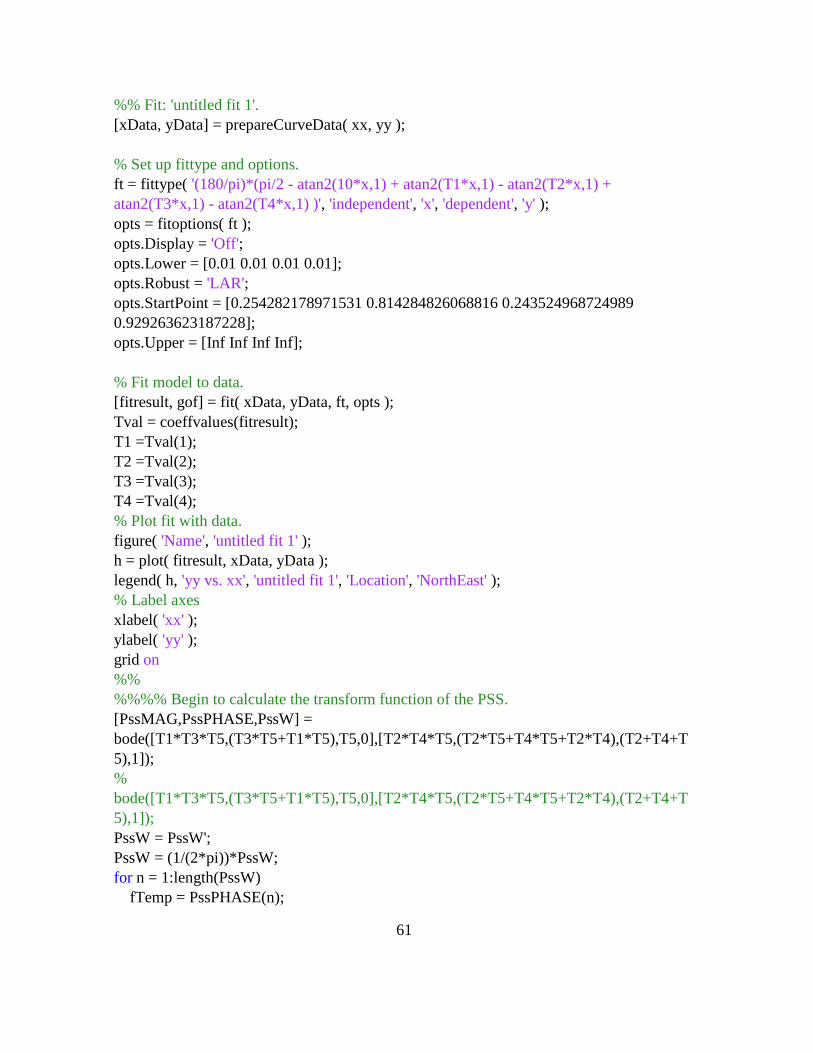
61
%% Fit: 'untitled fit 1'.
[xData, yData] = prepareCurveData( xx, yy );
% Set up fittype and options.
ft = fittype( '(180/pi)*(pi/2 - atan2(10*x,1) + atan2(T1*x,1) - atan2(T2*x,1) +
atan2(T3*x,1) - atan2(T4*x,1) )', 'independent', 'x', 'dependent', 'y' );
opts = fitoptions( ft );
opts.Display = 'Off';
opts.Lower = [0.01 0.01 0.01 0.01];
opts.Robust = 'LAR';
opts.StartPoint = [0.254282178971531 0.814284826068816 0.243524968724989
0.929263623187228];
opts.Upper = [Inf Inf Inf Inf];
% Fit model to data.
[fitresult, gof] = fit( xData, yData, ft, opts );
Tval = coeffvalues(fitresult);
T1 =Tval(1);
T2 =Tval(2);
T3 =Tval(3);
T4 =Tval(4);
% Plot fit with data.
figure( 'Name', 'untitled fit 1' );
h = plot( fitresult, xData, yData );
legend( h, 'yy vs. xx', 'untitled fit 1', 'Location', 'NorthEast' );
% Label axes
xlabel( 'xx' );
ylabel( 'yy' );
grid on
%%
%%%% Begin to calculate the transform function of the PSS.
[PssMAG,PssPHASE,PssW] =
bode([T1*T3*T5,(T3*T5+T1*T5),T5,0],[T2*T4*T5,(T2*T5+T4*T5+T2*T4),(T2+T4+T
5),1]);
%
bode([T1*T3*T5,(T3*T5+T1*T5),T5,0],[T2*T4*T5,(T2*T5+T4*T5+T2*T4),(T2+T4+T
5),1]);
PssW = PssW';
PssW = (1/(2*pi))*PssW;
for n = 1:length(PssW)
fTemp = PssPHASE(n);
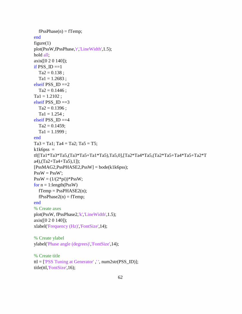
62
fPssPhase(n) = fTemp;
end
figure(1)
plot(PssW,fPssPhase,'r','LineWidth',1.5);
hold all;
axis([0 2 0 140]);
if PSS_ID ==1
Ta2 = 0.138 ;
Ta1 = 1.2683 ;
elseif PSS_ID ==2
Ta2 = 0.1446 ;
Ta1 = 1.2102 ;
elseif PSS_ID ==3
Ta2 = 0.1396 ;
Ta1 = 1.254 ;
elseif PSS_ID ==4
Ta2 = 0.1459;
Ta1 = 1.1999 ;
end
Ta3 = Ta1; Ta4 = Ta2; Ta5 = T5;
k1k6pss =
tf([Ta1*Ta3*Ta5,(Ta3*Ta5+Ta1*Ta5),Ta5,0],[Ta2*Ta4*Ta5,(Ta2*Ta5+Ta4*Ta5+Ta2*T
a4),(Ta2+Ta4+Ta5),1]);
[PssMAG2,PssPHASE2,PssW] = bode(k1k6pss);
PssW = PssW';
PssW = (1/(2*pi))*PssW;
for n = 1:length(PssW)
fTemp = PssPHASE2(n);
fPssPhase2(n) = fTemp;
end
% Create axes
plot(PssW, fPssPhase2,'k','LineWidth',1.5);
axis([0 2 0 140]);
xlabel('Frequency (Hz)','FontSize',14);
% Create ylabel
ylabel('Phase angle (degrees)','FontSize',14);
% Create title
ttl = ['PSS Tuning at Generator' ,' ', num2str(PSS_ID)];
title(ttl,'FontSize',16);
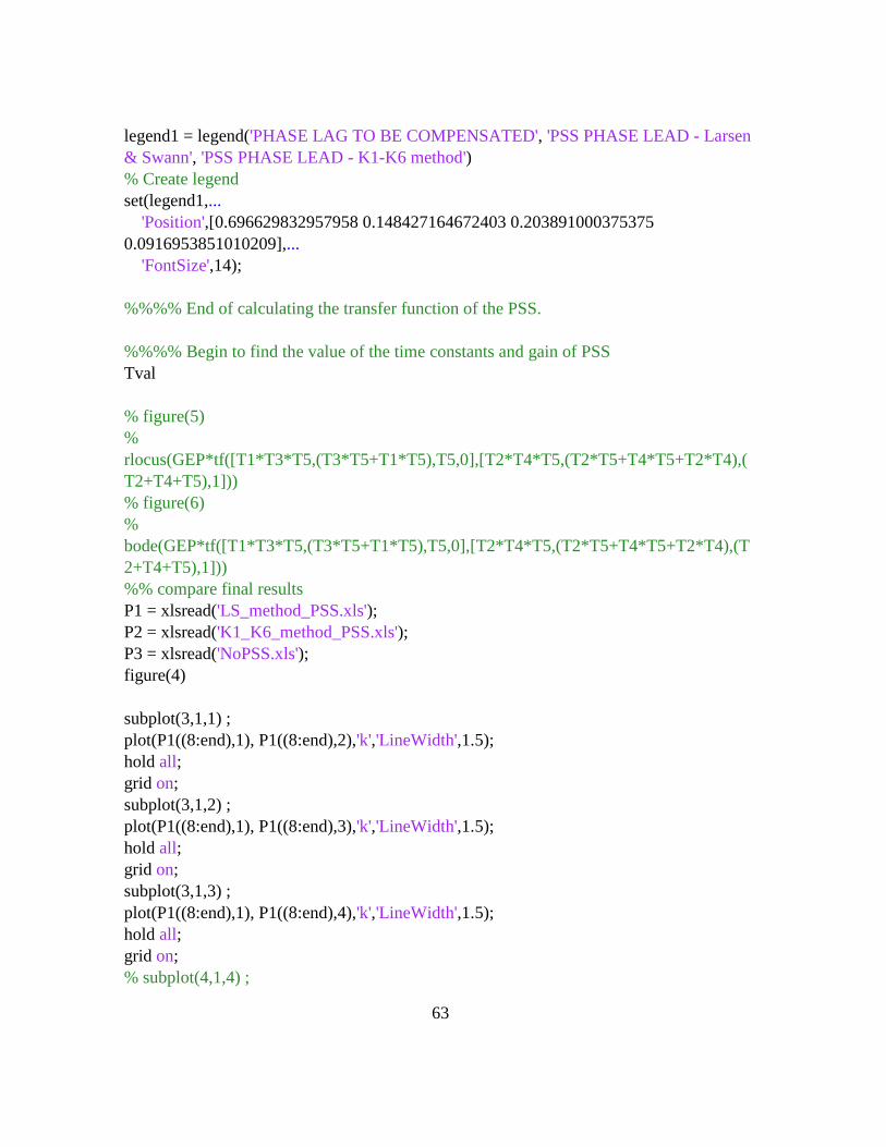
63
legend1 = legend('PHASE LAG TO BE COMPENSATED', 'PSS PHASE LEAD - Larsen
& Swann', 'PSS PHASE LEAD - K1-K6 method')
% Create legend
set(legend1,...
'Position',[0.696629832957958 0.148427164672403 0.203891000375375
0.0916953851010209],...
'FontSize',14);
%%%% End of calculating the transfer function of the PSS.
%%%% Begin to find the value of the time constants and gain of PSS
Tval
% figure(5)
%
rlocus(GEP*tf([T1*T3*T5,(T3*T5+T1*T5),T5,0],[T2*T4*T5,(T2*T5+T4*T5+T2*T4),(
T2+T4+T5),1]))
% figure(6)
%
bode(GEP*tf([T1*T3*T5,(T3*T5+T1*T5),T5,0],[T2*T4*T5,(T2*T5+T4*T5+T2*T4),(T
2+T4+T5),1]))
%% compare final results
P1 = xlsread('LS_method_PSS.xls');
P2 = xlsread('K1_K6_method_PSS.xls');
P3 = xlsread('NoPSS.xls');
figure(4)
subplot(3,1,1) ;
plot(P1((8:end),1), P1((8:end),2),'k','LineWidth',1.5);
hold all;
grid on;
subplot(3,1,2) ;
plot(P1((8:end),1), P1((8:end),3),'k','LineWidth',1.5);
hold all;
grid on;
subplot(3,1,3) ;
plot(P1((8:end),1), P1((8:end),4),'k','LineWidth',1.5);
hold all;
grid on;
% subplot(4,1,4) ;

64
% plot(P1((8:end),1), P1((8:end),5),'k','LineWidth',1.5);
% hold all;
% grid on;
figure(4)
subplot(3,1,1) ;
plot(P2((8:end),1), P2((8:end),2),'r','LineWidth',1.5);
subplot(3,1,2) ;
plot(P2((8:end),1), P2((8:end),3),'r','LineWidth',1.5);
subplot(3,1,3) ;
plot(P2((8:end),1), P2((8:end),4),'r','LineWidth',1.5);
% subplot(4,1,4) ;
% plot(P2((8:end),1), P2((8:end),5),'r','LineWidth',1.5);
figure(4)
subplot(3,1,1) ;
plot(P3((8:end),1), P3((8:end),2),'b','LineWidth',1.5);
title('Generator at bus#1');
xlabel('Time (s)');
ylabel('Rotor angle {\delta} (deg)');
legend('Larsen & Swann Method PSS Design', 'K1-K6 Method PSS Design','No PSS')
hold all;
subplot(3,1,2) ;
plot(P3((8:end),1), P3((8:end),3),'b','LineWidth',1.5);
title('Generator at bus#2');
xlabel('Time (s)');
ylabel('Rotor angle {\delta} (deg)');
legend('Larsen & Swann Method PSS Design', 'K1-K6 Method PSS Design','No PSS')
subplot(3,1,3) ;
plot(P3((8:end),1), P3((8:end),4),'b','LineWidth',1.5);
% subplot(4,1,4) ;
% plot(P3((8:end),1), P3((8:end),5),'b','LineWidth',1.5);
title('Generator at bus#4');
xlabel('Time (s)');
ylabel('Rotor angle {\delta} (deg)');
legend('Larsen & Swann Method PSS Design', 'K1-K6 Method PSS Design','No PSS')
%% compARE PLOTS at SS Limit
Pa1 = xlsread('compare at ss limit LS method.xls');
Pa2 = xlsread('compare at ss limit K1K6 method.xls');
% P3 = xlsread('NoPSS.xls');
figure(7)
subplot(3,1,1) ;
65
plot(Pa1((8:end),1), Pa1((8:end),2),'k','LineWidth',1.5);
hold all;
grid on;
subplot(3,1,2) ;
plot(Pa1((8:end),1), Pa1((8:end),3),'k','LineWidth',1.5);
hold all;
grid on;
subplot(3,1,3) ;
plot(Pa1((8:end),1), Pa1((8:end),4),'k','LineWidth',1.5);
hold all;
grid on;
% subplot(4,1,4) ;
% plot(P1((8:end),1), P1((8:end),5),'k','LineWidth',1.5);
% hold all;
% grid on;
figure(7)
subplot(3,1,1) ;
plot(Pa2((8:end),1), Pa2((8:end),2),'r','LineWidth',1.5);
title('Generator at bus#1');
xlabel('Time (s)');
ylabel('Rotor angle {\delta} (deg)');
legend('Larsen & Swann Method PSS Design', 'K1-K6 Method PSS Design','No PSS')
subplot(3,1,2) ;
plot(Pa2((8:end),1), Pa2((8:end),3),'r','LineWidth',1.5);
title('Generator at bus#2');
xlabel('Time (s)');
ylabel('Rotor angle {\delta} (deg)');
legend('Larsen & Swann Method PSS Design', 'K1-K6 Method PSS Design','No PSS')
subplot(3,1,3) ;
plot(Pa2((8:end),1), Pa2((8:end),4),'r','LineWidth',1.5);
title('Generator at bus#4');
xlabel('Time (s)');
ylabel('Rotor angle {\delta} (deg)');
legend('Larsen & Swann Method PSS Design', 'K1-K6 Method PSS Design')