evaluation of a mechanical stiffness...

i

1. Report No.

NM99MSC-07.2

2. Government Accession No. 3. Recipient's Catalog No.

5. Report Date

December 2001

4. Title and Subtitle

Evaluation of a Mechanical Stiffness Gauge for CompactionControl of Granular Media 6. Performing Organization Code

7. Author(s)

Lary R. Lenke, R. Gordon McKeen, Matt Grush

8. Performing Organization Report No.

10. Work Unit No. (TRAIS)9. Performing Organization Name and Address

ATR Institute University of New Mexico 1001 University Blvd., SE, Suite 103 Albuquerque, NM 87106

11. Contract or Grant No.

CO 3924

13. Type of Report and Period Covered

Final Report June 1999 - December 2001

12. Sponsoring Agency Name and Address

Research Bureau New Mexico State Highway & Transportation Department 7500 East Frontage Road P.O. Box 94690 Albuquerque, NM 87199-4690

14. Sponsoring Agency Code

15. Supplementary Notes

David Albright, NMSH&TD Research Bureau Chief; Rais Rizvi, NMSH&TD Research Engineer;Stan Matingly, FHWA Research & Technology Engineer; Steve Von Stein, FHWA Pavement Engineer.16. Abstract

The use of nuclear methods for compaction control is increasingly problematic for state highwayagencies. Regulatory and safety issues have prompted agencies such as the New Mexico State Highwayand Transportation Department to look for non-nuclear alternatives for compaction control. This reportdescribes the evaluation of one such commercially available device known as the GeoGauge. TheGeoGauge measures soil stiffness, arguably, a much more viable engineering parameter than themoisture-density relations currently used.

The GeoGauge was found to measure soil stiffness as advertised. Results relating moisture, density,and stiffness were found to be consistent with earlier research on compaction and mechanical strength ofsoils. However, because of the dynamic nature of the measurement obtained via the GeoGauge andassociated boundary constraints, the ability to obtain a target value for stiffness in the laboratory hasproved to be elusive.

Because of the promising nature of the GeoGauge technology, and because it measures a trueengineering mechanical property, a paradigm shift may be necessary for implementation for fieldcompaction control. Future specifications for compaction using this technology may require specificcontrols of moisture and requirements concerning compaction equipment with stiffness monitoring, viathe GeoGauge.

17. Key Words:

Compaction Control, GeoGauge, Moisture, Density,Soil Stiffness

18. Distribution Statement

Available from NMSH&TD Research Bureau

19. Security Classif. (of this report)

None

20. Security Classif. (of this page)

None

21. No. of Pages

58

22. Price

ii

EVALUATION OF A MECHANICAL STIFFNESS GAUGE FOR COMPACTIONCONTROL OF GRANULAR MEDIA

Prepared for:

Research BureauNew Mexico State Highway & Transportation Department

7500 East Frontage RoadP.O. Box 94690

Albuquerque, NM 87199-4690

Prepared by:

Lary R. LenkeR. Gordon McKeen

Matt Grush

ATR InstituteUniversity of New Mexico

1001 University Blvd., SE, Suite 103Albuquerque, NM 87106

December 2001

iii

ACKNOWLEDGEMENTS

Appreciation is extended to ATR Institute research staff who performed the field and

laboratory efforts described in this report. Mr. Tom Escobedo, Teaching Laboratory Supervisor,

and Mr. Kenny Martinez, Materials Laboratory Supervisor, performed much of the described

experimental efforts. Mr. Patrick Reser, undergraduate engineering student, assisted in the

experimental work as well. Mr. Kiran Pallachulla, engineering graduate student, is thanked for

helping with preparation of portions of the manuscript. Thanks to Ms. Jeanette Albany for her

expertise and advice in the use of MS Word and her editorial review. Special thanks are also

extended to the ATRI contract and procurement staff who help get the job done, especially Ms.

Geri Knoebel and Ms. Debby Pendell.

The research described herein was funded by the Research Bureau, New Mexico State

Highway and Transportation Department (NMSHTD). Thanks to Mr. David Albright, Bureau

Chief, and Mr. Rais Rizvi, Bureau Research Engineer. Also, thanks to Mr. Stan Mattingly,

Research Engineer, and Mr. Steven Von Stein, Pavement Engineer, FHWA, New Mexico

Division.

Thanks to Mr. Mel Main, of Humboldt Manufacturing, for suggestions and advice

regarding the experimental design and assisting with the data acquired and described in

Chapter VI.

iv

TABLE OF CONTENTS

I. INTRODUCTION …………………………………………………..……………………. 1

II. GEOGAUGE THEORY OF OPERATION ……………………………………………... 8

III. EVALUATION ON APPROXIMATE ELASTIC HALF SPACE OF DRY SAND …... 13

IV. EVALUATION ON COHESIVE SOIL ……….…………….…………………………. 26

V. STIFFNESS TARGET VALUE USING CYLINDRICAL PROCTOR MOLDS ……… 32

VI. FIELD STIFFNESS TESTING …………………………………………………………. 49

VII. CONCLUSIONS AND RECOMMENDATIONS ……………………………….……. 53

VIII. REFERENCES ……………………………………………………………………….. 55

v

LIST OF FIGURES

Figure 1. Strength and Density vs. Compactive Energy and Moisture Content (Seed & Chan).

Figure 2. Strength (CBR) and Density vs. Compactive Energy and Moisture Content (Turnbull& Foster).

Figure 3. GeoGauge Schematic and Cross-Section (Model H-4140).

Figure 4. Frequency Response Functions of Model Footings on Dry Sand, a) CylindricalContainer w/o Energy Absorbing Material, b) Cylindrical Container w/ EnergyAbsorbing Material, c) Cylindrical Container (Modified) w/ Energy AbsorbingMaterial, d) Cubical Container w/ Energy Absorbing Material (Lenke, et al).

Figure 5. Cubical Test Bin, Sand Raining Operation.

Figure 6. Cubical Test Bin, Stiffness Evaluation by GeoGauge.

Figure 7. Uniform Vertical Ring Loading on Surface of Elastic Half Space.

Figure 8. Vertical Stress Distribution Below an Annular Footing.

Figure 9. Cubical Test Bin, Layer Stiffness Evaluation by GeoGauge.

Figure 10. Boundary Effects Evaluation in Cubical Test Bin.

Figure 11. Stiffness vs. Distance to Vertical Boundary.

Figure 12. Plywood Soil Bin for Cohesive Soil (note compaction hammer).

Figure 13. GeoGauge Testing on Plywood Soil Bin with Cohesive Soil.

Figure 14. Moisture Content Evaluation (Full Depth).

Figure 15. Density and GeoGauge Stiffness vs. Moisture Content for Cohesive Soil.

Figure 16. GeoGauge Test on Soil on Concrete Pedestal (note acrylic mold).

Figure 17. GeoGauge Test on Soil on Concrete Floor (note steel mold).

Figure 18. GeoGauge Test Schematic for Tests on Soil in Modified Proctor Molds, a) Test onConcrete Pedestal, b) Test on Concrete Floor.

Figure 19. Pulse Velocity Measurements on Soil Within Proctor Mold.

Figure 20. Comparison of GeoGauge Measurement on Pedestal vs. Floor.

Figure 21. Comparison of Pulse Velocity Measurements (54 vs. 24 kHz).

Figure 22. Moisture Density Relations for All Soils.

Figure 23. Pulse Velocity Stiffness vs. Moisture Content for All Soils.

Figure 24. GeoGauge Stiffness vs. Moisture Content for All Soils.

Figure 25. Stress Waves Produced in a 5.5 by 5.5 by 0.25 inch “Perspex” Plate by a Charge ofLead Azide Explosive Detonated at the Center of the Upper Edge (times given aremeasured from the instant of detonation), 1) 0 µs, 2) 10.5 µs, 3) 21.7 µs, 4) 34.3 µs,5) 47.3 µs, 6) 60.8 µs, 7) 72.7 µs, 8) 84.7 µs, 9) 98.5 µs (Kolsky).

vi

LIST OF FIGURES (CONTINUED)

Figure 26. GeoGauge vs. Roller Passes, Base Course Material.

Figure 27. Field Measurements on Lime Stabilized Subgrade.

Figure 28. Field Stiffness vs. Time of Lime Stabilized Materials.

LIST OF TABLES

Table 1. Test Matrix for Target Value Determination Using Modified Proctor Molds

Table 2. Field Stiffness of Lime Stabilized Materials

1

I. INTRODUCTION

Compaction is the densification of soils by the application of mechanical energy. In

general it also involves the modification of the water content. Compaction control of bound and

unbound granular soils used in highway construction is necessary to improve their engineering

properties. There are several advantages, which occur through compaction, viz.,

1) Detrimental settlements can be reduced or prevented.

2) Soil strength increases and slope stability can be improved.

3) Bearing capacity of pavement subgrades, sub-bases, and base courses can be

improved.

4) Undesirable volume changes, for example, caused by frost action, swelling, and

shrinkage may be controlled.

Proctor established that compaction is a function of four variables (Holtz and Kovacs,

1981), viz., (1) dry density, (2) water content, (3) compactive effort, and (4) soil type. Consider

the common laboratory Proctor test (compaction test) wherein a given soil is compacted into a

standard mold with a given compaction energy at varied moisture contents. The classical

resultant graph of measured dry density versus moisture content is used to determine the

maximum density and optimum moisture content. 1 The maximum density and optimum

moisture content are used in specifications for highway construction to ensure proper compaction

of respective subgrades, sub-bases, and base courses.

While the Proctor test allows the determination of a field target value for compaction

control, the actual determination of in-situ density is commonly determined via destructive or

1 Standard procedures used are described in AASHTO T 99, and T 180, and ASTM D 698, andD1557.

2

non-destructive field control tests. Destructive tests involve the excavation and removal of some

of the intact granular fill material, whereas non-destructive tests determine the density and water

content of the granular soil indirectly. Common destructive methods employed are the sand cone

method (AASHTO T 191 (ASTM D 1556)), and the balloon density method (AASHTO T 205

(ASTM D 2167)).

Non-destructive determination of density and moisture content using radioactive isotopes

has been widely used in lieu of destructive methods for over twenty years now (AASHTO T 238

and T 239 (ASTM D 2922 and D 3017)). Nuclear methods have advantages over the past

traditional destructive techniques. Nuclear tests can be conducted rapidly with results known

within minutes. Such rapidity allows the contractor and field engineer to know the results

quickly, allowing corrective action to be taken as necessary before too much additional

earthwork has been placed. More tests per unit time allow a better statistical measure of the

compaction control process. Average values of density and moisture content are obtained over a

significantly larger volume of fill.

Disadvantages of nuclear methods include their relatively high initial cost and the

potential dangers of radioactive exposure to field personnel. Strict radiation safety and training

must be enforced with the use of nuclear devices.

The above-mentioned disadvantages of nuclear devices have prompted numerous

transportation agencies, including the New Mexico State Highway and Transportation

Department (NMSHTD), to look for non-nuclear methods for compaction control. Such

alternatives must eliminate the safety and regulatory concerns of nuclear methods, yet it is

desirable that any alternatives provide comparable speed and precision during field testing. This

desire precludes a step back to the old days of sand cone and balloon density measurements.

3

Any alternative must also provide a measurand 2 that is related to the engineering properties and

engineering performance of the soil evaluated.

The objective of compaction is to stabilize soils and improve their engineering behavior.

It is important to keep in mind the desired engineering properties of compacted earthwork, not

just its dry density and moisture content. This point is often lost in earthwork construction

control. Numerous studies have been performed over the years with regard to engineering

properties of soils and the influence of compaction on such properties (Seed and Chan, 1959,

Turnbull and McRae, 1950, Turnbull and Foster, 1956). These previous studies focused on

mechanical strength properties and how such mechanical properties are affected by compaction.

Figure 1 shows the work of Seed and Chan. It clearly shows the effects of compaction energy

and moisture content on the strength behavior of a compacted clay material. The strengths of

these clay materials tend to decrease, or roll off, as the molding moisture content is increased

past the optimum moisture content. Turnbull and Foster also found similar trends. Figure 2

shows a strength parameter (California Bearing Ratio (CBR)) versus compaction energy and

moisture content. Again, the CBR decreases as the molding moisture is increased beyond the

optimum moisture content for all compaction energies considered.

Typical compaction control specifications require densities that exceed some percentage

of the maximum dry density (e.g., 95% of maximum) and moisture contents that are a few

moisture content percentage points on either side of the optimum moisture content. Such

specifications help to ensure that the mechanical strength (an engineering property) is optimized

for a given soil. It is clear that the ubiquitous Proctor curve and field density measurements that

2 measurand – the physical quantity or property being measured (a technical term not found inyour typical English dictionary)

4

are in use today are, in reality, surrogate measurements that have evolved for ensuring optimal

mechanical performance of compacted soils. It is equally clear that such density measurements

have been used because of their simplicity and inexpensive nature when compared to more

sophisticated strength testing methods.

While strength is known to relate to dry density and moisture content for a given soil,

density and moisture content, nonetheless, are not good measures or predictors of engineering

properties. It is, however, recognized that material engineering properties such as strength are

related to soil stiffness (a mechanical property), which in turn is related to soil modulus (a

material property). The latter soil modulus is routinely used in elastic pavement design and

influences the pavement structural stiffness and resultant deflections under traffic loadings.

Hence, many researchers have focused on the use of simple techniques for measuring the soil

modulus or soil stiffness with regard to compaction control. Such stiffness measurements are

more fundamentally sound from an engineering perspective than the now universally accepted

moisture-density measurements used for compaction control.

The NMSHTD is interested in replacing nuclear devices because of the aforementioned

disadvantages of such devices. The ATR Institute at the University of New Mexico was asked

by the NMSHTD to identify off the shelf technology that has the potential to replace nuclear

devices. The ATR Institute focused on devices that have the ability to provide more meaningful

engineering properties, such as soil stiffness or soil modulus, and identified the Humboldt

GeoGauge (Stiffness Gauge) as the most promising alternative to nuclear devices. The

GeoGauge measures soil stiffness, which can in turn be used to calculate the soil modulus.

5

Figure 1. Strength and Density vs. Compactive Energy and Moisture Content (Seed & Chan).

6

Figure 2. Strength (CBR) and Density vs. Compactive Energy and Moisture Content (Turnbull& Foster).

7

This report documents an evaluation of the GeoGauge in both laboratory and field

environs. Chapter II describes the GeoGauge and its theory of operation. Chapter III presents a

laboratory evaluation of the GeoGauge using cohesionless dry silica sand. Chapter IV extends

the discussion of Chapter III to a similar evaluation of the GeoGauge on a cohesive soil.

Chapter V presents a detailed laboratory experiment that attempts to develop a procedure for

ascertaining field target values of stiffness. Chapter VI discusses some experiences with the

GeoGauge in actual field operations, including an evaluation of a lime-stabilized material.

Chapter VII provides a summary of conclusions and recommendations for further research aimed

at eventual implementation of the GeoGauge as a replacement for nuclear devices.

8

II. GEOGAUGE THEORY OF OPERATION

The GeoGauge, manufactured by the Humboldt Manufacturing Company, is a portable

instrument providing a simple and rapid means of measuring the stiffness of compacted

subgrade, subbase, and base course layers in earthen construction. The GeoGauge measures

stiffness at the soil surface by imparting very small displacements to the soil on an annularly

loaded region via a harmonic oscillator operating over a frequency of 100 to 196 Hz.

Appropriate transducer technology is incorporated to measure both force and displacement from

which stiffness can be computed. The computed stiffness is determined based on an average of

25 stiffness values obtained at 25 discreet frequencies over the frequency band cited above.

The GeoGauge weighs approximately 10 kg (22 lb). The annular ring which contacts the

soil has an outside diameter of 4.50 in. (114 mm) and an inside diameter of 3.50 in. (89 mm);

hence, with an annular ring thickness of 0.50 in. (13 mm). Humboldt specifications state that the

magnitude of the vertical displacement induced at the soil-ring interface is less than 0.00005 in.

(1.3 x 10 -6 m). The annular foot bears directly on the soil, supporting the weight of the

GeoGauge. Attached above this annular footing is a shaker, which excites the footing in a

vertical mode. Sensors attached to the shaker and footing are used to measure the force and

displacement from which soil stiffness is computed.

Figure 3 presents a schematic of the GeoGauge’s cross-section and salient features. The

heart of the mechanical system is an electro-mechanical shaker, which drives a flexible plate

attached via a rigid cylinder to the rigid annular foot. Matched velocity sensors attached to the

flexible plate (V2) and the rigid annular foot (V1) allow for the determination of the soil stiffness

in the following fashion. The force applied by the shaker (Fdr) and transferred to the soil beneath

9

the rigid foot (Fsoil) is measured by the differential displacement across the flexible plate as

follows:

)( 12 XXKFF flexsoildr −== (2-1)

where

drF = the force applied by the electro-mechanical shaker and transferred to the soil

flexK = the flexible plate stiffness

2X = the displacement of the flexible plate

1X = the displacement of the rigid annular foot.

Differentiation of Equation 1 in the time domain results in the following:

)( 12 VVKF flexsoil −=•

(2-2)

where

2V = the velocity of the flexible plate

1V = the velocity of the rigid annular foot.

Now, the soil stiffness (Ksoil) is simply

1X

FK soil

soil = (2-3)

with differentiation yielding

1V

FK

soil

soil

•

= (2-4)

10

Electro-MechanicalShaker

Flexible Plate

Velocity Sensor(Upper #2)

Velocity Sensor(Lower #1)

Rigid Cyl inder

Rigid Foot w/Annular Ring

Control & Display

External Case

Electronics

Vibration IsolationM o u n tP o w e r

SupplyV1

P o w e rSupply

2V

Fd r

Process Control & I /O

TestSignal

Calculat ion& Logg ing

Signal Process ing

Control & Display

Figure 3. GeoGauge Schematic and Cross-Section (Model H-4140).

Substitution of Equation 2-2 into Equation 2-4 yields an equation for soil stiffness in terms of the

measured velocities V1 and V2, and the stiffness flexK . 3

1

12 )(

V

VVKK flex

soil

−= (2-5)

11

As stated above, the GeoGauge measures the soil stiffness response at 25 discreet

frequencies and hence an average value of stiffness is determined ( soilK ) via the following

formula

∑ −=n

flexsoil V

VV

n

KK

1 1

12 )((2-6)

where n equals the number of test frequencies. The above described approach using velocity

measurements avoids the need for a non-moving reference for the soil displacement and permits

the accurate measurement of small displacements. The GeoGauge was designed assuming the

following condition exists, viz., at the frequencies of operation (100-196 Hz), the response is

dominated by the stiffness of the underlying soil (the manufacturer specifies a range of stiffness

measurement capability from 3 to 70 MN/m).

Figure 3 shows that the velocity transducer signals are processed on an onboard

microprocessor with subsequent calculation, logging, and data display. Output is via a user-

friendly face panel on the top of the GeoGauge. Power is supplied by six “D” cell batteries.

The measured soil stiffness from the GeoGauge can, in turn, be used to calculate the soil

modulus of the underlying bound or unbound soil media. The problem of a rigid annular ring on

a linear elastic, homogeneous, and isotropic half space has been considered by Egorov (1965).

The static stiffness K of such a soil-structure interaction problem has the functional form

)()1( 2 n

ERK

ων−= (2-7)

where E and ν are the modulus of elasticity and Poisson’s ratio of the elastic media, respectively,

R is the outside radius of the annular ring, and )(nω is a function of the ratio of the inside

3 flexK is known form established calibration procedures, defined by the manufacturer.

12

diameter and the outside diameter of the annular ring. For the ring geometry of the GeoGauge,

the parameter ω(n) is equal to 0.565, hence,

)1(

77.12ν−

= ERK (2-8)

Now, the modulus of elasticity and the shear modulus (G) are related through ( )ν+=

12

EG ,

hence, the above equation for stiffness can be expressed in terms of shear modulus as

( )ν−=

1

54.3 GRK (2-9)

These equations assume that the underlying soil is linear elastic, homogeneous, and

isotropic. They also assume an infinite half space. The assumptions of homogeneity, isotropy,

and elasticity are frequently invoked in soil mechanics and pavement design when analyzing soil

layers. However, the assumption of an infinite half space is arguably violated when one

considers that underlying pavement layers are generally of finite depth (on the order of 6 inches)

and are of increasing modulus with depth. Hence, any computation of elastic modulus from the

GeoGauge measured stiffness must be carefully evaluated in view of the above assumptions

made in the Egorov solution.

This section has briefly described the GeoGauge and its theory of operation. The

manufacturer states that the GeoGauge measures stiffness, which can in turn be related to an

engineering parameter such as modulus. Such a true engineering parameter is desirable in lieu of

surrogate measures such as density and moisture content.

13

III. EVALUATION ON APPROXIMATE ELASTIC HALF SPACE OF DRY SAND

A first step in evaluation of the GeoGauge is to determine if measured response on

known materials is consistent with both theoretical and empirical soil mechanics concepts. It is

desirable to evaluate the GeoGauge in a simple laboratory setup and use such theoretical and

empirical concepts to verify the stiffness response of the GeoGauge. Such laboratory studies can

be problematic except when using the most ideal soils. It has been found that dry uniform sized

sands can be used in such studies. However, when performing dynamic soil-structure interaction

studies (the GeoGauge and underlying soil are indeed a simple, albeit, small soil-structure

problem), one has to be concerned with boundary conditions, wave propagation concerns, and

reflected wave energy from near and distant boundaries.

Such dynamic soil-structure interaction experiments were conducted by Lenke, et al

(1991), at the University of Colorado, using model footings in an enhanced gravitational field,

using the geotechnical centrifuge modeling technique. Because of the inability to truly model an

elastic half space experimentally, they evaluated numerous container shapes and boundary

materials to minimize reflected wave energy in an attempt to approximate true radiation damping

of a vertically excited circular footing. One of the principal conclusions from their research was

that cubical containers with a compliant energy absorbing boundary material allowed reasonable

approximation of an elastic half space.

Figure 4 (from Lenke, et al) shows the effects of boundary shape and absorbing boundary

material on the response of a circular model footing. Figure 4a shows the measured frequency

response function for a model footing on the surface of dry sand contained within a cylindrical

14

aluminum container. 4 Figure 4b shows a similar experiment of the same footing on sand, but

with an energy absorbing boundary material on the inside surfaces of the aluminum container. It

is clear that the energy absorbing material reduces the energy spikes of the measured frequency

response function shown in Figure 4a. The energy absorbing material tends to prevent the

magnification or de-magnification (i.e., ringing) of reflected energy from the container

boundaries. Figure 3c shows an additional improvement in the response of the model footing by

further enhancements of the boundary geometry within the cylindrical container. Finally,

Figure 4d shows the effects of using an approximate cubical container lined with the same

energy absorbing material. The further improvement is marked, with the frequency response

being very close to the theoretical response as described in Lenke et al. The cubical container

geometry prevents focusing of transmitted and reflected energy to the source (i.e., the footing),

and further helps simulate an elastic half space.

In order to evaluate the GeoGauge, a similar approach was taken, albeit, on a larger scale

than the experiments conducted by Lenke, et al. A relatively large steel box was obtained of

approximate cubical shape. This steel container is lined with steel plate and reinforced

externally by steel channel sections, resulting in a fairly rigid container. The nominal

dimensions of this container are 24 in. (610 mm) deep with a lateral cross sectional area of 28 in.

by 30 in. (710 mm by 760 mm). The lateral and bottom surfaces of this container were lined

with 3/4 in. (19 mm) Styrofoam panels as an energy absorbing material.

4 A frequency response function (FRF) is a frequency domain representation of the input-outputrelation for a linear system (see Bendat and Piersol). The data shown in Figure 4 is essentially afrequency domain representation of a force input to a displacement output, i.e., stiffness, of afoundation on an elastic half-space with varied boundary conditions. The GeoGauge alsomeasures stiffness in the frequency domain and averages measured stiffness values over a fairlynarrow frequency band.

15

Figure 4. Frequency Response Functions of Model Footings on Dry Sand, a) CylindricalContainer w/o Energy Absorbing Material, b) Cylindrical Container w/ EnergyAbsorbing Material, c) Cylindrical Container (Modified) w/ Energy AbsorbingMaterial, d) Cubical Container w/ Energy Absorbing Material (Lenke, et al).

A dry granular cohesionless silica sand was obtained from U.S. Silica’s Ottawa, Illinois,

manufacturing facility. The sand selected was designated as F-52. The product information

provided by U.S. Silica states that this sand has a specific gravity of 2.65 (typical of silica sand)

with a round grain shape. The mean grain size is approximately 0.26 mm (0.010 in.) based on a

tabulated particle size distribution.

This silica sand was then pluviated through air from a height of 18 in. (460 mm) into the

foam lined steel test bin described above (see Figure 5). This “raining” operation took

approximately 20 hours to accomplish in order to ensure a uniform, highly compact granular

media within the test bed. Upon completion of the raining operation, the surface of the sand

media was carefully screeded level with the top of the test bin. During this operation the total

weight of material placed was carefully tracked. Based on careful measurement of the test bin

16

dimensions prior to pluviation of the sand, the resultant density of the media within the test bin

could be calculated. The average density (unit weight) computed was 110.45 lb/ft3 (1769.3 kg/

m3). Based on this unit weight and the known specific gravity, the void ratio of the granular

media within the test bin was computed as 0.497 (~100% relative density).

Figure 5. Cubical Test Bin, Sand Raining Operation.

With the granular media now in place within the test bin, measurements of stiffness were

obtained using the Humboldt GeoGauge (Figure 6). Measurements were obtained at the center

of the test bin surface as well as at quarter points along one diagonal of the square cross section.

A total of eight measurements were obtained on centerline with a mean value of

6.19 MN/m (35,300 lb/in.). The standard deviation of these eight measurements was

17

0.04 MN/m. The associated coefficient of variation, as defined by the ratio of the standard

deviation to the mean, was 0.7%.

Figure 6. Cubical Test Bin, Stiffness Evaluation by GeoGauge.

Hardin and Richart (1963) found that the modulus of rigidity (shear modulus) could be

related to the void ratio and the mean effective octahedral stress (i.e., average confining pressure)

by the following empirical equation.

( )( ) ( ) 5.0

2

1

17.22630oe

eG σ

+−= (2-10)

where G is the shear modulus, e is the void ratio of the granular media, and oσ is the mean

confining pressure (bulk stress). The above equation was developed for round-grained sands

using dynamic wave propagation experimental methods. The above equation is empirical and

has non-homogeneous units. The engineering units of both the shear modulus and mean

18

effective stress are in terms of pounds per square inch (psi) and apparently the numerical value

2630 has units of (psi)0.5.

Equation 2-10 can be used to calculate the stiffness defined previously in Equation 2-9 if

the unknown parameters can be estimated with some certainty. The void ratio in Equation 2-10

was very carefully determined during the experimental placement of the sand in the soil test bin.

The value of the mean effective stress is much more difficult to ascertain, however. In addition,

Poisson’s ratio in Equation 2-9 is not known. However, if one can estimate the values of the

mean effective stress and Poisson’s ratio, then Equations 2-9 and 2-10 can be used to estimate

the stiffness of the granular soil in the test bin and a comparison can be made with the GeoGauge

experimental value of 6.19 MN/m.

The mean effective stress can be computed using the following definition

( )ovvovhv

o KK

2133

2

3

2 +=+=+= σσσσσσ (2-11)

where vσ and hσ are the vertical and horizontal effective stress components, respectively, and

oK is the coefficient of lateral earth pressure. The value of oK can be estimated by an equation

developed by Jaky (1944)

+−

+=

φφφ

sin1

sin1sin

3

21oK (2-12)

where φ is the effective angle of internal friction of the granular media. An estimate of this

angle of internal friction was obtained by a simple experiment to determine the angle of repose

of the F-52 silica sand used in the bin test described previously. The angle of repose measured

was 33°. This is considered a lower bound for φ ; the actual value of φ may approach 40° but

the lower bound will be used for further computational analysis. Using the angle of repose as an

approximation for the internal angle of friction yields a coefficient of lateral earth pressure

19

of 0.402. Substitution of this value into Equation 2-11 yields the following for the mean

effective stress

vo σσ 601.0= (2-13)

It can be shown that Poisson’s ratio can be estimated using generalized Hooke’s law as

follows (Wood, 1990)

o

o

K

K

+=

1ν (2-14)

For the coefficient of lateral earth pressure previously estimated, the value of Poisson’s ratio is

calculated to be 0.287.

At this point, rational means have been used to estimate all variables for computing the

stiffness of the silica sand used in the bin tests with the exception of the vertical effective stress.

The value of this vertical effective stress is much more difficult to estimate. The effective stress

below the annular footing can be considered as composed of two components. One component

is the geostatic, or lithostatic, stress caused by the self-weight of the material. This vertical self-

weight component is simply the density (or unit weight) of the material (γ ) times the depth

below the footing (z). Essentially, the self-weight component of vertical stress is zero at the

ground surface of the soil bin and increases in a linear fashion with depth. The second

component of vertical stress is caused by the presence of the annular footing on the surface of the

experimentally modeled half space.

The analytical solution for the vertical stress distribution on centerline (σ v) below an

annularly loaded footing, at r = 0, is presented in Poulos and Davis (1974) as

( ) 2/522

33

za

apzv

+=σ (2-15)

20

where a is the distance from the center of the footing to the centerline of the ring (see Figure 7),

z is the depth below the centerline of the annular footing, and p is an annular line load acting at a

distance a from the centerline of the footing. For the GeoGauge used in the experiments

described previously, a is equal to 2.0 in. (51 mm), and the weight of the GeoGauge was

measured at 22.01 lb, resulting in an annular line load p of 1.752 lb/in. (306.8 N/m).

Line Loadingp / Unit Length

z

r

a

Figure 7. Uniform Vertical Ring Loading on Surface of Elastic Half Space.

Figure 8 shows a graphical representation of the vertical stress distribution as a function

of depth for both the geostatic stress component and the annular ring induced component. The

sum of these two stress components is the total vertical effective stress. The total stress

distribution clearly shows that the stress levels become fairly constant and uniform for depths of

2 to 9 inches (50 mm to 230 mm). It is well known that the “pressure bulb” below a circular

footing extends to a depth equal to about twice the diameter of the footing. The dynamic

response of the annular footing will also be influenced by a zone of soil to a depth of about two

diameters as well. Based on the observed total stress distribution of Figure 8 and a knowledge

21

that the depth of influence extends to two diameters (9 in.), an estimate of 0.63 psi is made for

the vertical effective stress below the annular footing.

Substitution of this estimated 0.63 psi vertical effective stress into Equation 2-13 with

subsequent substitution of this bulk stress into Equation 2-10 yields an estimate for the shear

modulus of the granular media within the soil test bin. This shear modulus along with the

previously estimated value of Poisson’s ratio and the outside radius of the GeoGauge annular

footing is then substituted into Equation 2-9 yielding a static stiffness of 33,800 lb/in.

Uniform Vertical Annular Line LoadCenter Line Stress @ r = 0(Line Load = 1.752 lb/in.,

Annular Radius, a = 2.0 in.)

0

3

6

9

12

15

18

21

24

0.00 0.40 0.80 1.20 1.60

Vertical Stress, psi

Dep

th, i

n.

Geostatic Stress

Load Induced Stress

Total Stress

Figure 8. Vertical Stress Distribution Below an Annular Footing.

22

Comparison of this computational estimate with the experimentally determined value of

stiffness (35,300 lb/in) results in an error less than 5%. Based on this simple experiment and a

rational soil mechanics analysis, one would conclude that the GeoGauge is indeed measuring the

stiffness of the underlying granular soil media.

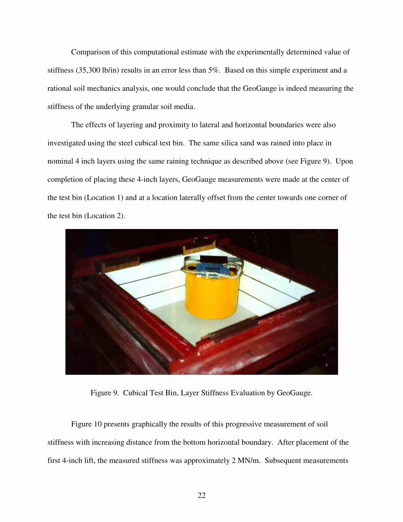
The effects of layering and proximity to lateral and horizontal boundaries were also

investigated using the steel cubical test bin. The same silica sand was rained into place in

nominal 4 inch layers using the same raining technique as described above (see Figure 9). Upon

completion of placing these 4-inch layers, GeoGauge measurements were made at the center of

the test bin (Location 1) and at a location laterally offset from the center towards one corner of

the test bin (Location 2).

Figure 9. Cubical Test Bin, Layer Stiffness Evaluation by GeoGauge.

Figure 10 presents graphically the results of this progressive measurement of soil

stiffness with increasing distance from the bottom horizontal boundary. After placement of the

first 4-inch lift, the measured stiffness was approximately 2 MN/m. Subsequent measurements

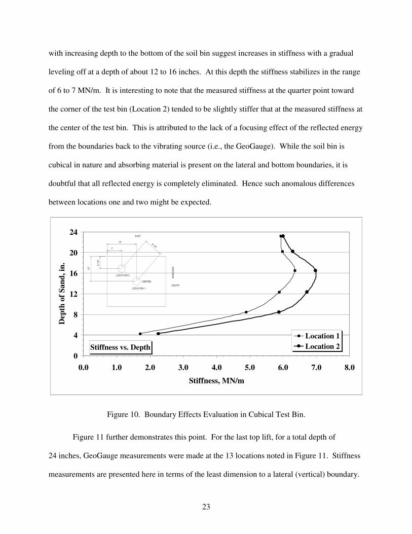
23

with increasing depth to the bottom of the soil bin suggest increases in stiffness with a gradual

leveling off at a depth of about 12 to 16 inches. At this depth the stiffness stabilizes in the range

of 6 to 7 MN/m. It is interesting to note that the measured stiffness at the quarter point toward

the corner of the test bin (Location 2) tended to be slightly stiffer that at the measured stiffness at

the center of the test bin. This is attributed to the lack of a focusing effect of the reflected energy

from the boundaries back to the vibrating source (i.e., the GeoGauge). While the soil bin is

cubical in nature and absorbing material is present on the lateral and bottom boundaries, it is

doubtful that all reflected energy is completely eliminated. Hence such anomalous differences

between locations one and two might be expected.

Stiffness vs. Depth0

4

8

12

16

20

24

0.0 1.0 2.0 3.0 4.0 5.0 6.0 7.0 8.0

Stiffness, MN/m

Dep

th o

f Sa

nd, i

n.

Location 1Location 2

CENTER

9 1/2"

13"

14"

LOCATION 2

LOCATION 1

6 1/

2"

7"

EAST

WIN

DO

WS

SOUTH

Figure 10. Boundary Effects Evaluation in Cubical Test Bin.

Figure 11 further demonstrates this point. For the last top lift, for a total depth of

24 inches, GeoGauge measurements were made at the 13 locations noted in Figure 11. Stiffness

measurements are presented here in terms of the least dimension to a lateral (vertical) boundary.

24

Locations 1, 5, 6, 9, 10, 11, 12, and 13 are all located at about 5.5 inches from the lateral

boundary. Locations 2, 4, 7, and 8 are located at the quarter points towards the corner of the test

bin (similar to Location 2 in Figure 10) at about 8 to 10 inches from the lateral boundaries.

Location 3 is in the center of the test bin (same as Location 2 in Figure 10) at a distance of

12.5 inches from any lateral boundary. Again it is clear that the GeoGauge response is

attenuated for measurements close to the lateral boundary. This is consistent with the

observations made previously with respect to the discussion of Figure 10. Stiffness

measurements stabilize at a lateral distance from the vertical boundary on the order of 8 to

10 inches.

Stiffness vs. Least DimensionSand Bin Layer 6 (Top Layer)

4.00

4.50

5.00

5.50

6.00

6.50

7.00

0 2 4 6 8 10 12

Least Dimension, in.

Stif

fnes

s, M

N/m

1 01

1 3 3

2

8

6

X

1 1

7

4

SOU T H

1 2

EA ST

Y

9 5

Figure 11. Stiffness vs. Distance to Vertical Boundary.

25

One can conclude based on these simple experiments that the GeoGauge provides

meaningful stiffness results when the distance to horizontal boundaries are on the order of

12 inches deep and the distance to any lateral boundaries is on the order of 9 inches. These

numbers are consistent with the GeoGauge manufacturer’s claims regarding the minimum layer

thickness that may be evaluated and the proximity of buried objects (e.g., metal pipe, concrete

structures, etc.).

26

IV. EVALUATION ON COHESIVE SOIL

One of the principle objectives, in implementing the GeoGauge for field compaction

control, is obtaining an objective method for determining an a priori target value for stiffness.

Ideally, such a target value should be a laboratory determined value, similar in scope and effort

to the methodology used in determining optimum moisture and maximum density. It is clear that

the large cubical bin described in the previous chapter is a very time consuming process for the

determination of a target value. Furthermore, dry cohesionless sand is never found in the real

world of highway construction and compaction control. Subgrades and base course materials are

compacted with moisture and tend to have at least some degree of cohesion. These soils lend

themselves to densification and increased stiffness by the typical field compaction techniques.

Furthermore, laboratory compaction techniques are still a viable method for simulating this field

compaction.

The use of the GeoGauge in the laboratory is still problematic because of the boundary

effects that have been discussed earlier. In the search for a laboratory standard for stiffness

measurement that can be translated to the field, some compromises are inevitable in order to

achieve a test method that is relatively quick to perform, yet provides some definition of stiffness

potential for a given soil. The evaluation of a more typical cohesive soil requires the use of a

scaled down version of the sand bin of the previous chapter. It is also desirable to ascertain the

relation between density, stiffness, and moisture content in a more reasonably sized soil

container.

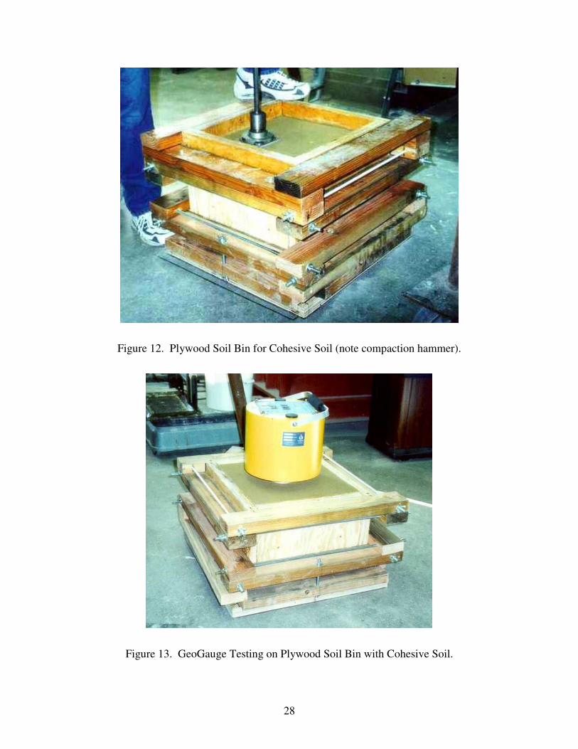
Thus, the first step in attempting to define a laboratory target value for stiffness using

cohesive soil was to use a smaller soil test container. A double plied reinforced plywood box,

with a wall and base thickness of 1.5 inch, was constructed with nominal dimensions of 15 inch

27

by 15 inch cross-section by 12 inch depth; a volume of 1.56 ft3. Plywood was selected for this

soil bin because of its superior energy absorbing properties compared to steel. Figure 12 shows

this soil container partially filled with compacted soil.

A cohesive silty-sand, an AASHTO A-2-4 material (Unified classification: SM), was

compacted into this soil bin using a standard Proctor compaction energy. A standard 10 pound

Marshall hammer, used for asphalt compaction, was modified with a 4 inch by 4 inch steel plate

attached to its base. Six lifts were compacted into the container to full depth. To achieve the

standard Proctor energy, the 10-pound hammer was dropped through its 18-inch drop height 228

times per lift. The last lift was trimmed flush with the top of the soil container for subsequent

testing by the GeoGauge. This described process was replicated for six different moisture

contents.

Figure 13 shows the actual testing with the GeoGauge on the surface of the cohesive soil.

After evaluation with the GeoGauge, the plywood sides were removed, and the sample was split

in half for moisture content evaluation (see Figure 14). Approximately 2 kg of soil was removed

from the internal section of these two halves along the entire depth of the sample for subsequent

drying and moisture content calculation.

The volume of soil for this test was markedly reduced compared to the sand bin tests

previously described, yet the effort to obtain one stiffness measurement with corresponding

density and moisture content was considerable. To obtain one set of measurements with

associated sample preparation, container assembly and disassembly takes in excess of 4 hours.

To obtain a complete set of stiffness and density parameters, for various moisture contents, takes

the better part of three man days.

28

Figure 12. Plywood Soil Bin for Cohesive Soil (note compaction hammer).

Figure 13. GeoGauge Testing on Plywood Soil Bin with Cohesive Soil.

29

Figure 14. Moisture Content Evaluation (Full Depth).

Figure 15 presents the results from evaluation of this cohesive silty-sand. The upper

graph shows the dry density versus moisture content. The maximum dry density is noted to be

116 lb/ft3 and the optimum moisture content is 12 %. In contrast to the density plot, the lower

graph shows that the maximum stiffness, as measured with the GeoGauge, is at a lower moisture

content. The maximum stiffness of 25 MN/m occurs at moisture content of about 7 %. This

“phase” shift is not surprising in view of the discussion presented in Chapter 1. Seed and Chan’s

work and that of Turnbull and Foster both suggest that peak mechanical response of a soil

material may peak before the point of optimum moisture content as defined in terms of dry

density. Their data clearly shows a “roll off” in mechanical response as the moisture content is

increased beyond the point of the peak mechanical response. The lower graph clearly shows this

“roll off” as the stiffness approaches zero at a moisture content of about 13 %.

30

The results of Figure 15 must be viewed with some judgment since the effects of the

lateral boundaries and focusing effects are not known. It is clear that this relatively small

container does not simulate the ideal elastic half space. However, the results are consistent with

previous studies cited in Chapter 1. The lower graph of Figure 15 suggests a “roll off” to zero

stiffness, which was observably not true, as the soil was still able to support its own weight upon

removal of the plywood forms (similar to the view of Figure 14). It is possible for the GeoGauge

to respond with a zero output, or even a negative stiffness value (which is physically impossible,

as stiffness by definition must be positive). Recall Equation 2-5 for the calculation of stiffness.

If the value of velocity transducer #1 is equal to or less than the value of velocity transducer #2,

then the GeoGauge measured (computed) stiffness will be zero or non-positive. Clearly when

this occurs, the GeoGauge is operating on a soil for which it was not designed or on a geometry

with boundary conditions for which it was not designed or intended, as well.

The other clear and obvious conclusion is that the development of a target value using the

described plywood soil bin is extremely time consuming for one soil let alone the numerous soils

expected on a typical construction project. Any laboratory procedure defined for obtaining a

stiffness target value must be accomplished in a time frame consistent with that necessary to

obtain the common Proctor density curve.

Figur

Lee Acres Silty SandStandard Proctor

Unified Classification: SMAASHTO Classification: A-2-4

104

106

108

110

112

114

116

118

120

0 5 10 15Moisture Content, %

Dry

Den

sity

, pcf

Lee Acres Silty SandStandard Proctor

Unified Classification: SMAASHTO Classification: A-2-4

0

5

10

15

20

25

30

0 5 10 15Moisture Content, %

Stiff

ness

, MN

/m

e 15. Density and GeoGauge Stiffness vs. Moisture Content for Cohesive Soil.

31

32

V. STIFFNESS TARGET VALUE USING CYLINDRICAL PROCTOR MOLDS

In view of the considerable time necessary to obtain a target value with the

aforementioned plywood soil bin, it was decided to attempt obtaining target values using

cylindrical proctor molds. Modified molds were chosen because of their larger internal diameter

of 6 inches in contrast with the more common standard proctor mold of 4-inch diameter. It

should be stated at the outset that this decision to obtain a target value with small molds is

fraught with concerns. It has been argued previously in this report that boundary concerns are

very real when making dynamic measurements. The closer the boundaries are to the excitation

source presents concerns about the value of the GeoGauge measurand and whether it is indeed

measuring the soil stiffness or some dynamic combination of the soil and proctor mold.

Nonetheless, such an experiment was undertaken because of the efficiency with which such

samples could be made and evaluated.

The GeoGauge measures stiffness in a 3-dimensional fashion based on the way wave

energy radiates from the vibrating source (foot). It was felt that an additional independent

dynamic measurement might be useful to corroborate or substantiate the GeoGauge

measurements. A one-dimensional wave propagation technique, commonly used for evaluating

portland cement concrete (ASTM C 597), was selected because of its simplicity. This

experimental technique, known as Pulse Velocity (PV) because of it one-dimensional

measurement, is minimally sensitive to the proctor mold constraining the soil material. As such,

the PV test can be used to ascertain the soil modulus as well as a stiffness that can be compared

to the GeoGauge measurement. The standard PV test used for concrete testing uses a pair of

54 kHz transducers. For the testing of soil in proctor molds, a pair of 24 kHz transducers was

33

also used to evaluate the subsequently described soils. The 24 kHz transducers are more suitable

for the lower modulus of soil and the finer particle sizes of soil in contrast to those of concrete.

The experiment is quite simple. Three soils were evaluated. Each soil was compacted

into modified steel proctor molds at varied moisture contents. In addition, to quantify the effects

of compaction energy, three different compaction energies were used on each soil as well. One

set of GeoGauge measurements were determined by placing the proctor mold with soil on a

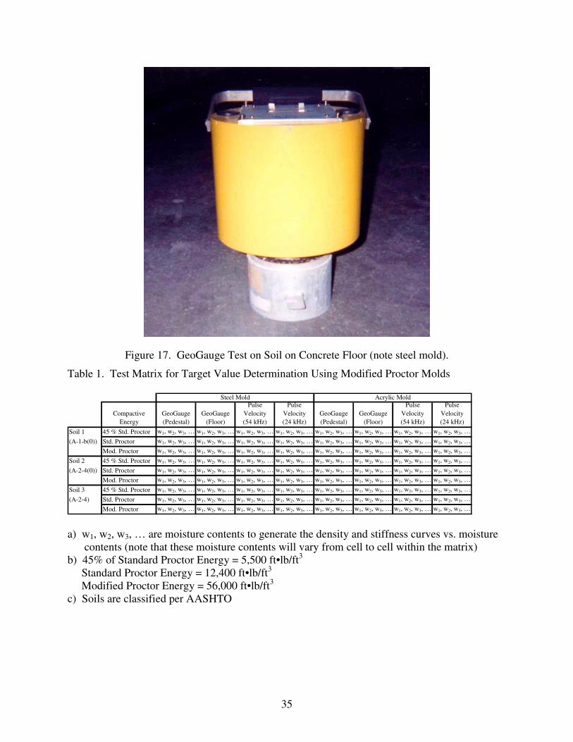
concrete pedestal (see Figure 16). A second set of GeoGauge measurements were obtained by

placing the mold with soil on a concrete floor (see Figure 17). In addition to GeoGauge stiffness

and PV measurements using 24 and 54 kHz transducers, density and moisture were carefully

measured as well. Lastly, because of concerns about the appropriateness of steel molds, the

same experiment was also conducted on molds made of acrylic. Table 1 shows the complete test

matrix employed.

Figure 18 is a schematic showing the two GeoGauge test configurations. The first

configuration is the evaluation of stiffness in a Proctor mold attached to a concrete pedestal.

Note the presence of the customary base plate attached to the concrete pedestal and the wing nuts

used to clamp a retainer plate at the top of the proctor mold (these are clearly visible in

Figure 16). The second configuration where the soil in the proctor mold is placed on the

concrete floor shows that any clamping or restraint of the mold was not employed.

Three soils were evaluated during this experiment. Soil #1 is a free-draining sandy

material used for mechanically stabilized earth wall construction. It is classified as an AASHTO

A-1-b(0). Soils #2 and #3 are silty-sandy materials used for compacted subgrade, classified as

A-2-4(0) and A-2-4 materials, respectively. All three soils were obtained during construction

activity from the reconstruction of the I-25 and I-40 interchange in Albuquerque, New Mexico.

34

Figure 16. GeoGauge Test on Soil on Concrete Pedestal (note acrylic mold).

35

Figure 17. GeoGauge Test on Soil on Concrete Floor (note steel mold).

Table 1. Test Matrix for Target Value Determination Using Modified Proctor Molds

a) w1, w2, w3, … are moisture contents to generate the density and stiffness curves vs. moisturecontents (note that these moisture contents will vary from cell to cell within the matrix)

b) 45% of Standard Proctor Energy = 5,500 ft•lb/ft3

Standard Proctor Energy = 12,400 ft•lb/ft3

Modified Proctor Energy = 56,000 ft•lb/ft3

c) Soils are classified per AASHTO

CompactiveEnergy

GeoGauge(Pedestal)

GeoGauge(Floor)

Pulse Velocity(54 kHz)


GeoGauge(Pedestal)

GeoGauge(Floor)



Soil 1 45 % Std. Proctor w1, w2, w3, … w1, w2, w3, … w1, w2, w3, … w1, w2, w3, … w1, w2, w3, … w1, w2, w3, … w1, w2, w3, … w1, w2, w3, …

(A-1-b(0)) Std. Proctor w1, w2, w3, … w1, w2, w3, … w1, w2, w3, … w1, w2, w3, … w1, w2, w3, … w1, w2, w3, … w1, w2, w3, … w1, w2, w3, …

Mod. Proctor w1, w2, w3, … w1, w2, w3, … w1, w2, w3, … w1, w2, w3, … w1, w2, w3, … w1, w2, w3, … w1, w2, w3, … w1, w2, w3, …


(A-2-4(0)) Std. Proctor w1, w2, w3, … w1, w2, w3, … w1, w2, w3, … w1, w2, w3, … w1, w2, w3, … w1, w2, w3, … w1, w2, w3, … w1, w2, w3, …



(A-2-4) Std. Proctor w1, w2, w3, … w1, w2, w3, … w1, w2, w3, … w1, w2, w3, … w1, w2, w3, … w1, w2, w3, … w1, w2, w3, … w1, w2, w3, …


Steel Mold Acrylic Mold

36

a) Concrete Pedestal b) Concrete Floor

Figure 18. GeoGauge Test Schematic for Tests on Soil in Modified Proctor Molds, a) Test onConcrete Pedestal, b) Test on Concrete Floor.

The different soils were compacted into 6-inch diameter modified proctor molds made of

steel or plastic at varied moisture contents. The essence of AASHTO test method T 180 was

followed during the varied compaction processes. The standard Proctor effort of 12,400 ft•lb/ft3

was achieved by placing 3 lifts and compacting each lift 56 times with a 5.5 lb hammer dropped

from a 12 inch height. The 45 % of standard Proctor effort of 5,500 ft•lb/ft3 was obtained by

placing 3 lifts and compacting each lift 25 times with a 5.5 lb hammer dropped from a 12-inch

height. The modified Proctor effort of 56,000 ft•lb/ft3 (~450 % of standard Proctor effort) was

achieved by placing 5 lifts and compacting each lift 56 times with a 10 lb hammer dropped from

a height of 18 inches. After compacting each sample, GeoGauge and PV measurements were

made along with density and moisture content determinations.

37

The pulse velocity measurements were obtained on the soil within the proctor molds as

depicted in Figure 19. The bottom transducer is placed on a set of slotted plates for egress of the

instrumentation cable. The soil sample within the Proctor mold is then centered on top of this

bottom transducer. The top transducer is then placed on top of the soil specimen. To ensure a

consistent contact pressure between the transducers and the soil specimen, a 2 kg slotted plate is

placed on top of the top transducer. The PV device measures the transit time of one-dimensional

pulses from one transducer to the other transducer. When the distance between the transducers is

known (the sample length in this case), the velocity of the pulse can be computed as follows

tLVd = (5-1)

where

dV = the dilatational wave speed of the soil

L = the soil specimen length (4.58 in)

t = the measured transit time of the one-dimensional pulse.

Because of the lateral constraint of the Proctor mold, the computed pulse velocity is considered

to be dilatational velocity as opposed to a rod velocity (an unconstrained velocity).

The above determined dilatational velocity can be used to compute what is known as a

constrained modulus (related for isotropic materials to the Young’s modulus or shear modulus)

as follows

2dVC ρ= (5-2)

where

C = the constrained modulus

ρ = the mass density of the soil specimen (note: this is not the unit weight or dry

density, but the mass per unit volume).

38

The dilatational velocity can also be used to compute the Young’s modulus of elasticity

(E) for an assumed value of Poisson’s ratio (ν) via the following equation

)1(

)21)(1(2

νννρ

−−+= dV

E (5-3)

For computations where this Young’s modulus of elasticity is determined based on pulse

velocity measurements, Poisson’s ratio is assumed equal to 0.35.

The constrained modulus can be converted to a soil stiffness value by the following

equation

L

CAK = (5-4)

where A equals the cross-sectional area of the soil specimen. Presenting the pulse velocity

measurements in terms of soil stiffness allows for a more ready comparison with the soil

stiffness values obtained with the GeoGauge.

39

Figure 19. Pulse Velocity Measurements on Soil Within Proctor Mold.

It is worthwhile to compare the difference between GeoGauge measurements made on

the concrete floor versus those made on the concrete pedestal. Figure 20 presents graphs for

both the steel mold and acrylic mold tests for all three soils compacted and tested at a standard

Proctor energy. These graphs suggest that there is little difference between modulus

determinations made on the two different concrete surfaces. The pedestal appears to be about

10% stiffer based on linear regression, but the scatter is sufficiently high to make this slight

difference insignificant. Comparison of these two graphs also suggests that there is little

difference between the measurements made in steel versus acrylic molds; most of the

measurements for both steel and acrylic were between 0.04 and 0.10 GPa. The modulus values

40

shown in this figure were computed using Equation 2-8 for an assumed value of Poisson’s ratio

of 0.35. Graphs for the other two compaction energies produce similar results and conclusions.

A similar comparison of pulse velocity measurements using 24 and 54 kHz transducers is

shown in Figure 21. One can conclude from these graphs that there is little difference, for

practical purposes, between the 24 and 54 kHz transducers for the soils evaluated. Again the

magnitudes of Young’s modulus between the steel and acrylic molds appear to be insignificant.

Both the GeoGauge measured stiffness and computed PV stiffness are mechanical

properties. As such, it is expected that these stiffness values will vary with moisture content and

compactive effort in a fashion similar to those discussed in Chapter 1 (Seed & Chan and

Turnbull & Foster). It was shown earlier that there is no practical significant difference between

GeoGauge measurements on a concrete floor compared to a concrete pedestal, or significant

differences between pulse velocity transducers (24 kHz vs. 54 kHz), or significant differences

between steel and acrylic Proctor molds. Therefore, the discussion to follow will be limited to

GeoGauge test results obtained on the concrete pedestal, pulse velocity measurements obtained

using the 54 kHz transducer pairs, and compaction performed in the steel Proctor molds.

Figure 22 shows the moisture-density relations obtained for the three soils using the three

different compaction energies. Note that the different compaction energies result in clearly

distinguishable loci. This is true for each of the three soils, as would be expected, and is

consistent with the classical references cited previously in Chapter 1. Also note that the data for

Soil #1 is not as spread out with respect to density (sensitive to compactive effort) as for the

other two soils. This is expected for a sandy soil in contrast to the cohesive Soils #2 and #3.

One would also expect that a mechanical property plotted versus moisture content would

result in very distinguishable loci for different compaction energies. Figure 23 shows plots of

41

pulse velocity stiffness versus the moisture content for the three soils evaluated. This figure

clearly shows that the mechanical property being measured by the pulse velocity technique is

sensitive to compaction energy. The only soil for which this is problematic is for Soil #1 which,

being a sandy material, is not very sensitive to density changes with different compaction energy,

and hence not very sensitive to stiffness change with different compaction energy. Figure 23

clearly shows that as the compaction energy is increased there is a corresponding increase in

stiffness at a given moisture content. Again, this is quite consistent with the work cited earlier

(Seed and Chan, Turnbull and Foster).

Figure 24 shows measured GeoGauge stiffness versus moisture content for the three soils

evaluated at three different compaction energies, in similar fashion to Figure 23. One would

expect that the loci of points representing different compaction energies would be quite distinct

and separate. This is not the case. For some moisture contents, the stiffness measurements of

the soil compacted with modified effort are less than that for the same soil compacted with the

sub-standard, 45 %, effort. There is no clear trend, for any of the three soils evaluated, of

increasing stiffness with increasing compaction energy as would be expected. Viewing the three

graphs suggest that the peak stiffness measurements for all three soils are essentially the same; in

the range of 8 to 12 MN/m. It’s not clear that the stiffness measurements are those of the soil or

of some combined effect of the soil, proctor mold, and bottom boundary configuration. It is

clear, though, that the GeoGauge as used in this configuration is unable to discriminate an

increase in stiffness with an increase in compaction energy. One can only conclude that trying to

obtain a stiffness target value on a volume of soil comparable in size to the foot of the GeoGauge

is not possible.

42

Standard Proctor CompactionAcrylic Mold

GeoGauge, All Soils

y = 1.0913x + 0.0031R2 = 0.936

0.00

0.02

0.04

0.06

0.08

0.10

0.12

0.00 0.02 0.04 0.06 0.08 0.10 0.12

EFloor (GPa)

EP

edes

etal

(G

Pa)

GeoGauge Comparison

Linear (GeoGauge Comparison)

1:1 Line

Standard Proctor CompactionSteel Mold

GeoGauge, All Soils

y = 1.0829x + 0.0001R2 = 0.8922

0.00

0.02

0.04

0.06

0.08

0.10

0.12

0.00 0.02 0.04 0.06 0.08 0.10 0.12

EFloor (GPa)

EP

edes

etal

(G

Pa)

GeoGauge Comparison

Linear (GeoGauge Comparison)

1:1 Line

Figure 20. Comparison of GeoGauge Measurement on Pedestal vs. Floor.

43

Standard Proctor CompactionAcrylic Mold

Pulse Velocity, All Soils

y = 0.9971x - 0.0491R2 = 0.9173

0.0

0.1

0.2

0.3

0.4

0.5

0.6

0.0 0.1 0.2 0.3 0.4 0.5 0.6

E24 kHz (GPa)

E54

kH

z (G

Pa)

Pulse Velocity Comparison

Linear (Pulse VelocityComparison)

1:1 Line

Standard Proctor CompactionSteel Mold

Pulse Velocity, All Soils

y = 1.0246x - 0.0422

R2 = 0.9518

0.0

0.1

0.2

0.3

0.4

0.5

0.6

0.0 0.1 0.2 0.3 0.4 0.5 0.6

E24 kHz (GPa)

E54

kH

z (G

Pa)

Pulse Velocity Comparison

Linear (Pulse VelocityComparison)

1:1 Line

Figure 21. Comparison of Pulse Velocity Measurements (54 vs. 24 kHz).

44

Soil #1Proctor Compaction

Steel Mold

105

110

115

120

125

130

135

0 2 4 6 8 10 12 14 16 18

Moisture Content, %

Dry

Den

sity

, pcf

Standard Effort

Modified Effort

45% Std. Effort


Steel Mold

105

110

115

120

125

130

135

0 2 4 6 8 10 12 14 16 18

Moisture Content, %

Dry

Den

sity

, pcf

Standard Effort

Modified Effort

45% Std. Effort


Steel Mold

105

110

115

120

125

130

135

0 2 4 6 8 10 12 14 16 18

Moisture Content, %

Dry

Den

sity

, pcf

Standard Effort

Modified Effort

45% Std. Effort

Figure 22. Moisture Density Relations for All Soils.

45


Steel Mold54 kHz Pulse Velocity Transducer

0

10

20

30

40

50

60

70

80

90

100

0 2 4 6 8 10 12 14 16 18

Moisture Content, %

Stif

fnes

s, M

N/m

Standard Energy

Modified Energy

45% Std. Energy



0

20

40

60

80

100

120

140

160

180

0 2 4 6 8 10 12 14 16 18

Moisture Content, %

Stif

fnes

s, M

N/m

Standard Energy

Modified Energy

45% Std. Energy



0

20

40

60

80

100

120

140

160

180

0 2 4 6 8 10 12 14 16 18

Moisture Content, %

Stif

fnes

s, M

N/m

Standard Energy

Modified Energy

45% Std. Energy

Figure 23. Pulse Velocity Stiffness vs. Moisture Content for All Soils.

46


Steel MoldGeoGauge (Pedestal)

0

2

4

6

8

10

12

0 2 4 6 8 10 12 14 16 18

Moisture Content, %

Stif

fnes

s, M

N/m

Standard Effort

Modified Effort

45% Std. Effort



0

2

4

6

8

10

12

14

16

0 2 4 6 8 10 12 14 16 18

Moisture Content, %

Stif

fnes

s, M

N/m

Standard Effort

Modified Effort

45% Std. Effort



0

2

4

6

8

10

12

14

0 2 4 6 8 10 12 14 16 18

Moisture Content, %

Stif

fnes

s, M

N/m

Standard Effort

Modified Effort

45% Std. Effort

Figure 24. GeoGauge Stiffness vs. Moisture Content for All Soils.

47

The main concern for obtaining a target value for a dynamic stiffness measurement, such

as the GeoGauge, is one of boundary conditions and focusing of reflected wave energy from

these boundaries back to the source (i.e., the vibrating annular foot). The wave energy bouncing

around in the small volume of the Proctor mold is quite complex, and surely chaotic in nature.

Wave energy is reflected and refracted off of the lateral boundaries as well as off the horizontal

bottom and top boundaries (the top boundary being the annular footing). In addition, the soil is

surely not uniform throughout the soil volume and layering effects due to the compaction process

make uniformity even more questionable. Density within layers is not constant and even the

thickness of individual specimens can vary and surely will vary between different specimens.

Symmetry of the GeoGauge on the surface of the Proctor specimen will also produce

non-symmetric and chaotic wave reflections. The ratio of the diameter of the foot of the

GeoGauge to the diameter of the Proctor mold is 0.75. The aforementioned experiments of

Lenke, et al made use of model footings less than 10% the size of the soil container, and

reflected wave energy was of considerable concern without the use of energy absorbing material

on the container boundaries.

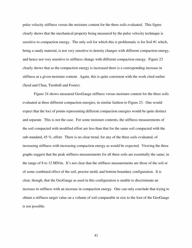
The above considerations, all verbiage, are perhaps illustrated best with a simple

illustrative example. Figure 25 shows an analogous geometry demonstrating the complex nature

of wave propagation in a very finite volume (Kolsky, 1953). This figure shows the propagation

of wave energy from a point source on the edge of a Perspex (acrylic) plate, a very uniform and

homogeneous material. This point source is a small charge of lead azide explosive at the center

of the upper edge (analogous to the annular line load of the GeoGauge). The right edge of each

photo within Figure 25 is analogous to the centerline (line of symmetry) of the GeoGauge. The

48

Perspex plate represents the underlying soil. It is also worthwhile to note that acrylic has

mechanical elastic properties, both modulus and Poisson’s ratio, similar to that of soil.

At 10.5 µs and at 21.7 µs the expanding wave front is radially symmetric and well

behaved. At 34.3 µs the wave front impinges on the left boundary (equivalent to the Proctor

mold boundary) and right boundaries (centerline of the GeoGauge) and both compressional and

shear wave energy is reflected off of these boundaries. At 60.8 µs the wave front hits the bottom

boundary (equivalent to the bottom of the Proctor mold) and is reflected as well. By 93.5 µs the

nature of the wave energy is obviously quite complicated, and this is only one cycle of

excitation. The GeoGauge is exciting such an upper boundary as the Perspex plate 100 to 200

times per second. Clearly the wave fronts propagating from such a source are interacting in a

very complex and chaotic fashion. Hence, it is not surprising that the response of the GeoGauge

on soil with similar boundary conditions is not well behaved and provides stiffness values that

are not consistent with known theory as the compaction energy is varied.

49

Figure 25. Stress Waves Produced in a 5.5 by 5.5 by 0.25 inch “Perspex” Plate by a Charge ofLead Azide Explosive Detonated at the Center of the Upper Edge (times given aremeasured from the instant of detonation), 1) 0 µs, 2) 10.5 µs, 3) 21.7 µs, 4) 34.3 µs,5) 47.3 µs, 6) 60.8 µs, 7) 72.7 µs, 8) 84.7 µs, 9) 98.5 µs (Kolsky).

50

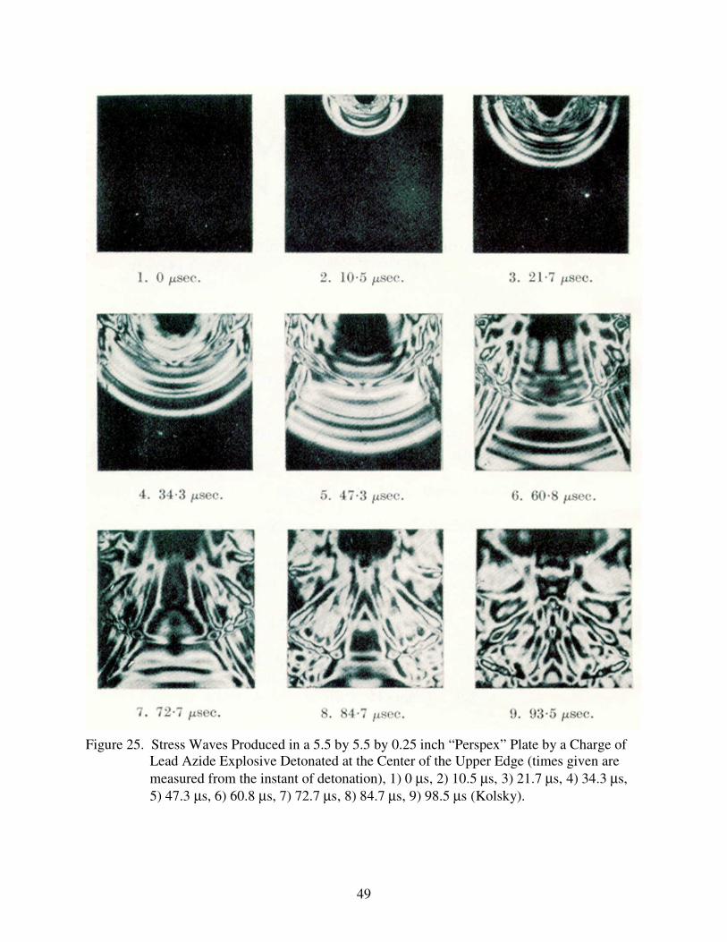
VI. FIELD STIFFNESS TESTING

The major thrust of this report has focused on laboratory evaluation. A limited amount of

field experimentation was conducted. In view of the fact that the GeoGauge cannot discriminate

between compaction energies when tested on a small volume of soil within a Proctor mold, it

was felt necessary to verify if the GeoGauge can discriminate stiffness increases in the field as

compaction progresses.

The GeoGauge was used to evaluate stiffness increase as a function of roller passes on a

base course material on an approach ramp on the Big-I (I-25 & I-40) reconstruction. The

approach ramp evaluated was the west bound to north bound ramp. Six locations on this ramp

were monitored via GeoGauge stiffness measurements as compaction occurred. Figure 26 shows

a plot of measured stiffness versus the number of roller passes. The roller was a steel wheeled

vibratory roller. Figure 26 clearly shows that the stiffness increased with the number of roller

passes. In contrast to the laboratory, the GeoGauge can indeed discriminate increases in stiffness

with increased compactive effort during field use.

An additional field data set was obtained on the reconstruction of New Mexico State

Highway 44 (now designated as U.S. 550). Lime stabilization was used extensively during this

reconstruction project to stabilize subgrade materials. Four distinct locations (stations), with

similar soil, were identified for GeoGauge stiffness evaluation. One location was used as a

control with no lime stabilization, the other three locations had been stabilized with lime and had

cured in-situ for different periods of time; the first for one day, the second for 2 days, and the

third for two weeks (14 days). Twenty-one (21) stiffness measurements were made at each

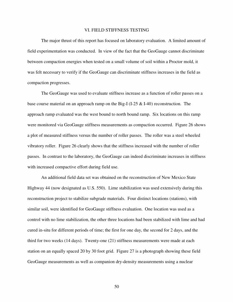
station on an equally spaced 20 by 30 foot grid. Figure 27 is a photograph showing these field

GeoGauge measurements as well as companion dry-density measurements using a nuclear

51

density device. Table 2 shows the results of this study. Note that the mean stiffness increases

with curing age for these lime stabilized materials. The variation of GeoGauge measurements

across the test grid is quite reasonable as indicated by the fairly low coefficient of variations.

Also note that the dry density at each location is the same regardless of curing age indicating that

stiffness is a good indicator of strength gain of these stabilized materials, while density clearly is

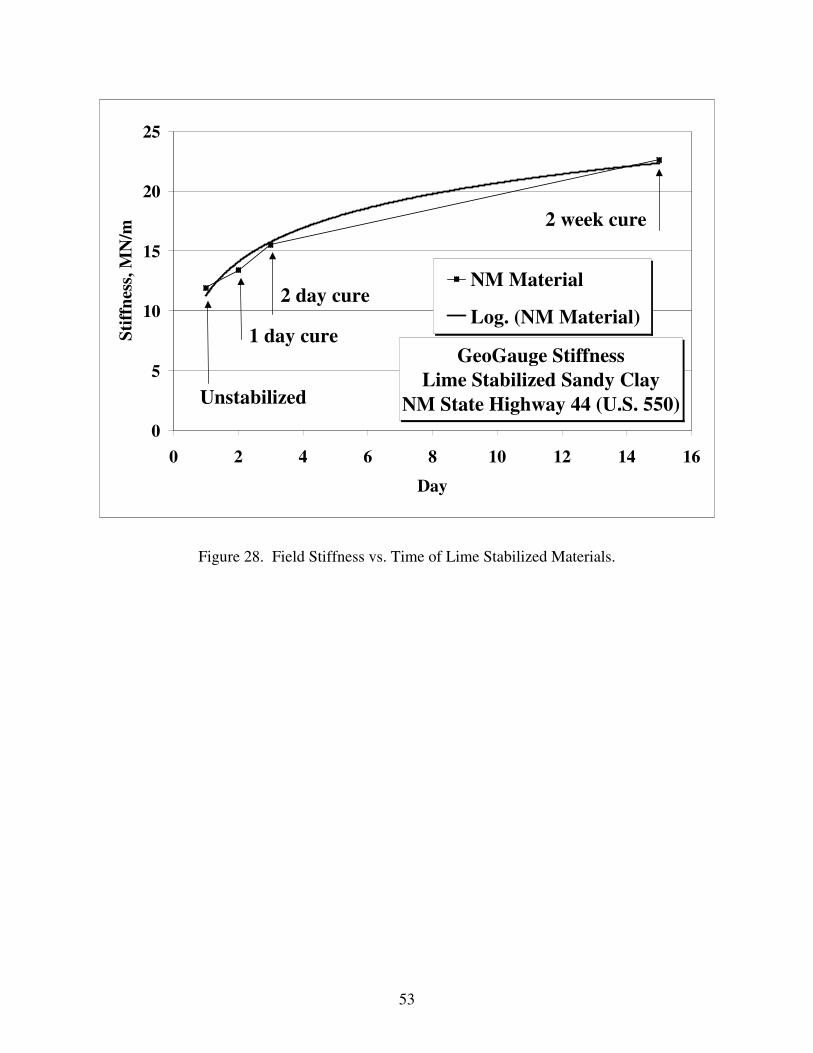
not. Figure 28 presents graphically the results of this table. Again it is clear that stiffness, and

therefore strength, increases with time during this curing process of lime stabilized materials.

Such use of the GeoGauge in these applications appears to be compelling.

Figure 26. GeoGauge vs. Roller Passes, Base Course Material.

GeoGauge Stiffness vs. No. of Roller PassesVibratory Roller

Big-I (I-25 & I-40 Interchange)West Bound to North Bound Ramp

Base Coarse @ Finish Grade1 October 2001

0.0

2.0

4.0

6.0

8.0

10.0

12.0

14.0

16.0

18.0

0 1 2 3 4 5 6 7 8 9

No. Roller Passes

Geo

Gau

ge S

tiff

ness

, MN

/m

Location #1

Location #2

Location #3

Location #4

Location #5

Location #6

52

Figure 27. Field Measurements on Lime Stabilized Subgrade.

Table 2. Field Stiffness of Lime Stabilized Materials

Location (Sta.) Age (day) Mean Std. Dev. COV (%) Dry Density (pcf)

4815* 0 11.9 1.7 14.1 102.3

5045 1 13.4 2.5 18.3 101.5

5045 2 15.5 2.6 16.9 101.5

5050 14 22.6 3.1 13.5 101.0

*Unstabilized

Lime Stabilized Sandy Clay - NM State Highway 44 (U.S. 550)Stiffness Test Results

Stiffness (MN/m)

53

GeoGauge StiffnessLime Stabilized Sandy Clay

NM State Highway 44 (U.S. 550)0

5

10

15

20

25

0 2 4 6 8 10 12 14 16

Day

Stif

fnes

s, M

N/m

NM Material

Log. (NM Material)

Unstabilized

1 day cure

2 day cure

2 week cure

Figure 28. Field Stiffness vs. Time of Lime Stabilized Materials.

54

VII. CONCLUSIONS AND RECOMMENDATIONS

The Humboldt GeoGauge appears to have real potential as an alternative non-nuclear

method for compaction control of highway materials. This study found that the GeoGauge does

indeed measure soil stiffness as advertised. This was verified using classical theoretical and

empirical soil mechanics concepts. Tests on cohesive soil showed that the soil stiffness does

indeed vary with moisture content, consistent with concepts first shown by Turnbull and Foster

and later by Seed and Chan. The optimum moisture for maximum stiffness does not in general

coincide with the optimum moisture content for maximum density.

The quest for a laboratory method for determining a field target value for stiffness

remains elusive, however. Attempts to ascertain a target value using modified Proctor molds

were not successful because of boundary effects caused by the small volume of soil in relation to

the size of the GeoGauge annular foot.

Field tests clearly show that stiffness increases can be observed with increasing

compaction as evidenced by monitoring of roller passes. This is encouraging and suggests that

implementation of the GeoGauge might be possible, albeit, with a substantial paradigm shift

away from lab evaluation to appropriate field monitoring of compaction processes. Field tests

also clearly show that stabilized materials evidence stiffness, and hence strength gains, over time.

The GeoGauge can be a useful tool for monitoring such stiffness gains, but again the use of

a priori laboratory stiffness data will be difficult, if not impossible, to develop for comparison

purposes.

In the absence of a laboratory determined target value for stiffness in the field, future

specifications, using GeoGauge like technology, may include careful control of moisture (still

determined by the common Proctor test), along with well-defined field compaction procedures

55

and equipment. Such prescriptive specifications, along with monitoring of stiffness with the

GeoGauge as compaction progresses, will result in maximum stiffness of subgrades, subbases,

and base course materials at optimal moisture contents. The use of stiffness for control of

compaction processes in the field, in contrast to current density control, will hopefully ensure

superior, more uniform, and longer lasting pavement systems.

The use of a test strip, on a given project soil, to establish compaction control parameters

using the GeoGauge may prove to be an acceptable alternative to the more conventional method

of knowing the target value a priori. Such an approach would likely still require knowledge of

moisture requirements (perhaps from the traditional Proctor test) and perhaps a specification of

compaction equipment. However, compaction effort and rolling patterns would be determined in

the field and GeoGauge stiffness determined corresponding to this established and agreed upon

compactive effort. This GeoGauge stiffness value would then be the target, or specification

value, for that soil for the duration of the project. Clearly, variability of the compaction process

and the GeoGauge measurements would have to be considered in establishing this field specified

stiffness.

56

VIII. REFERENCES

AASHTO T 99, Standard Method of Test for Moisture-Density Relations of Soils Using a 5.5 lb(2.5 kg) Rammer and an 12 in. (305 mm) Drop, Standard Specifications for TransportationMaterials and Methods of Sampling and Testing, American Association of State Highwayand Transportation Officials, Washington, DC, Part II, Tests.

AASHTO T 180, Standard Method of Test for Moisture-Density Relations of Soils Using a 10 lb(4.54 kg) Rammer and an 18 in. (457 mm) Drop, Standard Specifications for TransportationMaterials and Methods of Sampling and Testing, American Association of State Highwayand Transportation Officials, Washington, DC, Part II, Tests.

AASHTO T 191, Standard Method of Test for Density of Soil In-Place by the Sand-ConeMethod, Standard Specifications for Transportation Materials and Methods of Sampling andTesting, American Association of State Highway and Transportation Officials, Washington,DC, Part II, Tests.

AASHTO T 205, Standard Method of Test for Density of Soil In-Place by the Rubber-BalloonMethod, Standard Specifications for Transportation Materials and Methods of Sampling andTesting, American Association of State Highway and Transportation Officials, Washington,DC, Part II, Tests.

AASHTO T 238, Standard Method of Test for Density of Soil and Soil-Aggregate in Place byNuclear Methods (Shallow Depth), Standard Specifications for Transportation Materials andMethods of Sampling and Testing, American Association of State Highway andTransportation Officials, Washington, DC, Part II, Tests.

AASHTO T 239, Standard Method of Test for Moisture Content of Soil and Soil-Aggregate inPlace by Nuclear Methods (Shallow Depth), Standard Specifications for TransportationMaterials and Methods of Sampling and Testing, American Association of State Highwayand Transportation Officials, Washington, DC, Part II, Tests.

ASTM C 597, Standard Test Method for Pulse Velocity Through Concrete, Annual Book ofASTM Standards, American Society for Testing and Materials, West Conshohocken, PA,Vol. 4.02.

ASTM D 698, Standard Test Method for Laboratory Compaction Characteristics of Soil UsingStandard Effort (12,400 ft•lb/ft3 (600 kN•m/m3)), Annual Book of ASTM Standards,American Society for Testing and Materials, West Conshohocken, PA, Vol. 4.08.

ASTM D 1556, Standard Test Method for Density and Unit Weight of Soil in Place by theSand-Cone Method, Annual Book of ASTM Standards, American Society for Testing andMaterials, West Conshohocken, PA, Vol. 4.08.

57

ASTM D 1557, Standard Test Method for Laboratory Compaction Characteristics of Soil UsingModified Effort (56,000 ft•lb/ft3 (2,700 kN•m/m3)), Annual Book of ASTM Standards,American Society for Testing and Materials, West Conshohocken, PA, Vol. 4.08.

ASTM D 2167, Standard Test Method for Density and Unit Weight of Soil in Place by theRubber Balloon Method, Annual Book of ASTM Standards, American Society for Testingand Materials, West Conshohocken, PA, Vol. 4.08.

ASTM D 2922, Standard Test Methods for Density of Soil and Soil-Aggregate in Place byNuclear Methods (Shallow Depth), Annual Book of ASTM Standards, American Society forTesting and Materials, West Conshohocken, PA, Vol. 4.08.

ASTM D 3017, Standard Test Method for Water Content of Soil and Rock in Place by NuclearMethods (Shallow Depth), Annual Book of ASTM Standards, American Society for Testingand Materials, West Conshohocken, PA, Vol. 4.08.

Bendat, J.S., and Piersol, A.G., Random Data: Analysis and Measurement Procedures, 2nd Edit.,John Wiley and Sons, New York, 1986, p. 30.

Egorov, K.E., Calculation of Bed for Foundation with Ring Footing, Proc. 6th InternationalConference of Soil Mechanics and Foundation Engineering, Vol. 2, 1965, pp. 41-45.

Hardin, B.O., and Richart, F.E., Jr., Elastic Wave Velocities in Granular Soils, Journal of the SoilMechanics and Foundation Engineering Division, American Society of Civil Engineers,Vol. 89, No. SM1, 1963, pp. 33-65.

Holtz, R.D., and Kovacs, W.D., An Introduction to Geotechnical Engineering, Prentice-Hall,Englewood Cliffs, New Jersey, 1981.

Jaky, J., The Coefficient of Earth Pressure at Rest, Journal of the Union of Hungarian Engineersand Architects, 1944, pp. 355-358 (in Hungarian).

Kolsky, H., Stress Waves in Solids, Clarendon Press, Oxford, 1953 (Dover, New York, 1963).

Lenke, L.R., Pak, R.Y.S., and Ko, H-Y, Boundary Effects in Modeling Foundations Subjected toVertical Excitation, Proc. International Conference Centrifuge 1991, Balkema, Rotterdam,1991, pp. 473-480.

Poulos, H.G., and Davis, E.H., Elastic Solutions for Soil and Rock Mechanics, Wiley, New York,1974, p. 32.

Turnbull, W.J., and Foster, C.R., Stabilization of Materials by Compaction, Journal of the SoilMechanics and Foundations Division, American Society of Civil Engineers, Vol. 82, No.SM2, 1956, pp. 934-1 to 934-23.

58

Turnbull, W.J., and McRae, J.L., Soil Test Results Shown Graphically, EngineeringNews-Record, Vol. 144, 1950, pp. 38-39.

Seed, H.B., and Chan, C.K., Structure and Strength Characteristics of Compacted Clays, Journalof the Soil Mechanics and Foundations Division, American Society of Civil Engineers,Vol. 85, No. SM5, 1959, pp. 87-128.

Wood, D.M., Soil Behaviour and Critical State Soil Mechanics, Cambridge University Press,1990.

59

THIS PAGE INTENTIONALLY LEFT BLANK

evaluation of a mechanical stiffness...

Documents