California State University, San Bernardino California State University, San Bernardino

CSUSB ScholarWorks CSUSB ScholarWorks

Electronic Theses, Projects, and Dissertations Office of Graduate Studies

12-2018

EVALUATION OF A SEQUENTIAL POND SYSTEM FOR DETENTION EVALUATION OF A SEQUENTIAL POND SYSTEM FOR DETENTION

AND TREATMENT OF RUNOFF AT SKYPARK, SANTA'S VILLAGE AND TREATMENT OF RUNOFF AT SKYPARK, SANTA'S VILLAGE

Elizabeth Caporuscio

Follow this and additional works at: https://scholarworks.lib.csusb.edu/etd

Part of the Environmental Indicators and Impact Assessment Commons, Environmental Monitoring

Commons, Hydrology Commons, Natural Resources and Conservation Commons, Natural Resources

Management and Policy Commons, and the Water Resource Management Commons

Recommended Citation Recommended Citation Caporuscio, Elizabeth, "EVALUATION OF A SEQUENTIAL POND SYSTEM FOR DETENTION AND TREATMENT OF RUNOFF AT SKYPARK, SANTA'S VILLAGE" (2018). Electronic Theses, Projects, and Dissertations. 773. https://scholarworks.lib.csusb.edu/etd/773

This Thesis is brought to you for free and open access by the Office of Graduate Studies at CSUSB ScholarWorks. It has been accepted for inclusion in Electronic Theses, Projects, and Dissertations by an authorized administrator of CSUSB ScholarWorks. For more information, please contact scholarworks@csusb.edu.

EVALUATION OF A SEQUENTIAL POND SYSTEM FOR DETENTION AND

TREATMENT OF RUNOFF AT SKYPARK, SANTA’S VILLAGE

A Thesis

Presented to the

Faculty of

California State University,

San Bernardino

In Partial Fulfillment

of the Requirements for the Degree

Master of Science

in

Earth and Environmental Sciences

by

Elizabeth Mary Caporuscio

December 2018

EVALUATION OF A SEQUENTIAL POND SYSTEM FOR DETENTION AND

TREATMENT OF RUNOFF AT SKYPARK, SANTA’S VILLAGE

A Thesis

Presented to the

Faculty of

California State University,

San Bernardino

by

Elizabeth Mary Caporuscio

December 2018

Approved by:

James Noblet, Committee Chair, Chemistry

Jennifer Alford, Committee Member

Kerry Cato, Committee Member

© 2018 Elizabeth Mary Caporuscio

iii

ABSTRACT

Understanding the extent to which human activities impact surface water

resources has become increasingly important as both human population growth

and related landscape changes impact water quality and quantity across varying

geographical scales. Skypark, Santa’s Village is a 233.76-acre tourism-based

outdoor recreation area located in Skyforest, California residing within the San

Bernardino National Forest. The park is situated at Hooks Creek, the headwaters

of the Mojave River Watershed, and is characterized by a diverse landscape that

includes forest cover and human development, including impervious surfaces, a

restored meadow, and recreational trails. In 2016, Hencks Meadow was

considered degraded by human activity and restored by the Natural Resources

Conservation Services (NRCS) using best management practices (BMPs) to

manage stormwater runoff and mitigate pollutants entering recreational

downstream surface water. Three BMP detention basins were constructed to

store and improve water quality from stormwater runoff. The purpose of this

study is to observe the extent to which the engineered BMP detention basins

design were effective in mitigating stormwater pollution from entering Hooks

Creek. Over a six to eight month period (January to August), ponds were tested

in situ bi-weekly for temperature (ºC), dissolved oxygen (mg/L), pH, turbidity

(NTU), conductivity (µS/cm), nitrate (mg/L), and ammonium (mg/L), with

additional laboratory tests for total suspended solids (mg/L), total dissolved solids

(mg/L), chemical oxygen demand (mg/L), total coliform (MPN/100mL),

iv

Escherichia coli (MPN/100mL), and trace metals (µg/L). The results of this study

support that the BMP design is improving surface stormwater runoff from

impervious surfaces before it enters Hooks Creek. Findings could also promote

the design and implementation of stormwater BMP detention basins at other site

locations where water degradation is evident. Furthermore, this research can be

used to promote the necessary improvement of water quality and quantity on a

widespread geographical scale.

v

ACKNOWLEDGEMENTS

I would like to thank both my Co-Chairs Dr. Jennifer Alford and Dr. James

Noblet for their time, guidance, and effort throughout my project. I want to thank

my committee member Dr. Kerry Cato. I also want to thank Bill Johnson, the

owner of Skypark, for allowing access to the meadow and contribution to the

environmental restoration and conservation project.

I also want to thank my parents, Carol and Tom, and my siblings,

Courtney and Thomas for their support, encouragement, and motivation

throughout my academic career.

vi

TABLE OF CONTENTS

ABSTRACT ........................................................................................................... iii

ACKNOWLEDGEMENTS ..................................................................................... v

LIST OF TABLES ................................................................................................ viii

LIST OF FIGURES ............................................................................................... ix

CHAPTER ONE: INTRODUCTION

Literature Review ........................................................................................ 1

Land Types and Water Quality ........................................................ 2

Land Changes and Water Quality .................................................... 7

Human Impacts and Water Quality .................................................. 9

Hydrological Network and Water Quality ....................................... 12

Implementing Best Management Practices ................................... 13

Study Purpose and Objectives ...................................................... 19

CHAPTER TWO: STUDY SITE ........................................................................... 22

CHAPTER THREE: METHODS

Water Quality Testing ............................................................................... 28

Sampling Procedures .................................................................... 31

Data Analysis ................................................................................. 33

CHAPTER FOUR: RESULTS ............................................................................. 35

CHAPTER FIVE: DISCUSSION

Water Quality Parameters ........................................................................ 59

Water Temperature ........................................................................ 60

Dissolved Oxygen .......................................................................... 60

vii

pH .................................................................................................. 62

Turbidity ......................................................................................... 62

Conductivity ................................................................................... 63

Nitrate ............................................................................................ 64

Ammonium ..................................................................................... 64

Total Suspended Solids ................................................................. 65

Total Dissolved Solids ................................................................... 65

Chemical Oxygen Demand ............................................................ 66

Total Coliform ................................................................................ 66

E. coli ............................................................................................. 66

Trace Metals .................................................................................. 68

CHAPTER SIX: CONCLUSIONS ........................................................................ 69

APPENDIX A: TABLES ....................................................................................... 71

APPENDIX B: FIGURES ..................................................................................... 81

REFERENCES .................................................................................................... 99

viii

LIST OF TABLES

Table 1. Land Use Ranges in the Hydrologic Catchment Area ........................... 26 Table 2. Water Quality Criteria and Objectives ................................................... 36 Table 3. Pond 1 Descriptive Statistics and Exceedances ................................... 37 Table 4. Pond 2 Descriptive Statistics and Exceedances ................................... 38 Table 5. Pond 3 Descriptive Statistics and Exceedances ................................... 39 Table 6. Pond 4 Descriptive Statistics and Exceedances ................................... 40 Table 7. EPA Aquatic Life Criteria for Trace Metals ............................................ 41

ix

LIST OF FIGURES

Figure 1. Site Location Skypark Google Earth Image ......................................... 23

Figure 2. Mojave River Watershed ...................................................................... 24

Figure 3. NRCS Constructed Sediment Basins and Waterways ......................... 29

Figure 4. Daily Total Precipitation (In.) ................................................................ 42

Figure 5. Column Graph of Water Temperature (°C) .......................................... 45

Figure 6. Column Graph of Dissolved Oxygen (mg/L) ........................................ 46

Figure 7. Column Graph of pH ............................................................................ 47

Figure 8. Column Graph of Turbidity (NTU) ........................................................ 48

Figure 9. Column Graph of Conductivity (µS/cm) ................................................ 49

Figure 10. Column Graph of Nitrate (mg/L) ......................................................... 50

Figure 11. Column Graph of Ammonium (mg/L) ................................................. 51

Figure 12. Column Graph of Total Suspended Solids (mg/L) ............................. 52

Figure 13. Column Graph of Total Dissolved Solids (mg/L) ................................ 53

Figure 14. Column Graph of Chemical Oxygen Demand (mg/L) ........................ 54

Figure 15. Column Graph of Total Coliform (MPN/100mL) ................................. 55

Figure 16. Column Graph of E. coli (MPN/100mL) .............................................. 56

Figure 17. Column Graph of Chromium (µg/L) .................................................... 57

Figure 18. Column Graph of Lead (µg/L) ............................................................ 58

1

CHAPTER ONE

INTRODUCTION

Literature Review

Water resources are essential to sustaining human and aquatic health,

economic activities, and food and water security across local, regional, and

global geographical scales (Dwight et al., 2002; Gleick, 1998; Hunter et al., 2010;

Peters and Meybeck, 2009; Thoradeniya et al., 2017; Zhai et al., 2017). Over the

past several decades water resources have become adversely impacted by

climatic changes, land uses (e.g. urban, rural, and agricultural), human activities

(e.g. impervious surfaces, farming, and clearcutting), and failing water

infrastructure (e.g. wastewater treatment and septic systems) (Cahoon et al.,

2006; Corrao et al., 2015; Ensign and Mallin, 2001; Grimm et al., 2008; Holland

et al., 2004; Peters and Meybeck, 2009; Zimmerman et al., 2008). Water quality

and quantity impairments have been linked to human population growth that

often results in alterations to landscapes and hydrologic systems (Gleick, 1998;

Holland et al., 2004; Mallin et al., 2000; Zimmerman et al., 2008). When

considering these relationships across a hydrological landscape (e.g. river basin

or watershed), sources of water pollution may be highly variable and related to

natural systems, landscape features, and human activities (Alford et al., 2016;

Holland et al., 2004; St-Hilaire et al., 2015). Several studies have indicated that

the percent land type (e.g. urban, agricultural, and forest) and types of activities

on the landscape (e.g. crop production, livestock, and fertilizer applications) can

2

have variable influences on surface water including alterations of loads and

concentrations of pollutants (e.g. nutrients, bacteria, and metals) (Cahoon et al.,

2006; Ensign and Mallin, 2001; Genito et al., 2002; Lenat and Crawford, 1994).

For example, the increase of nutrients and bacteria from fertilizers, pesticides,

and human and animal waste on agriculture and urban landscapes can impact

water quality and quantity both locally and downstream from pollution sources

(Alford et al., 2016; Burkholder et al., 2007; Booth and Jackson, 1997; and

others). Significant increases in nutrients (e.g. phosphorus and nitrogen) create

eutrophic conditions resulting in the overproduction of plants, algae, and

decaying matter that often lead to a decrease in dissolved oxygen levels. Such

conditions cause disruptions in ecological services and reduce aquatic

biodiversity. In addition, people that come into contact with polluted surface

waters may experience adverse human health conditions including respiratory

complications and other infectious diseases (Arnold and Gibbons, 1996; Billen et

al., 2001; Burkholder et al., 1997; Carpenter et al., 1998; Heaney et al., 2015;

Hooiveld et al., 2016; Mallin et al., 2000; Manuel, 2014; Wilson and Serre, 2007).

The identification of relationships between specific landscape features and

activities and water quality is paramount to protecting and sustaining water

resources for current and future generations.

Land Types and Water Quality

Urban and agricultural landscapes have been identified as having various

impacts to surface water resources when compared to natural landscapes.

Although variable, natural landscapes including stream riparian areas are

3

typically void of human interaction and pollution inputs into water resources are

minimal (Lowrance et al., 1997). More recently, natural landscapes have

transitioned into urban and agricultural watersheds often characterized by

increased development of impervious surfaces due to the construction of roads,

buildings, and parking lots. Natural hydrologic systems are impacted when

impervious surfaces create barriers that do not allow rainfall to naturally infiltrate

into the soil and recharge groundwater. Stormwater infrastructure also impacts

water quality because it conveys runoff from rainfall to surface water systems in a

short period of time, increasing flood events and pollutant inputs on local and

regional scales across the hydrological network (Braune and Wood, 1999).

Specific pollutant inputs typically associated with urban areas include trace

metals, suspended solids, nutrients (e.g. nitrogen and phosphorus), and bacteria

(Dwight et al., 2002). Sources of pollutant inputs from urban areas include metals

from car exhaust, nutrients from lawn fertilizers, and bacteria from unsewered

developments and pet waste (Carpenter et al., 1998; Hathaway et al., 2009; Jia

et al., 2013; Mallin et al., 2000; NWQI, 2002; Olding et al., 2004; St-Hilaire et al.,

2015). In addition, watersheds with large percentages of agricultural lands

contribute nonpoint source pollution of nutrients from fertilizers and pesticides,

and bacteria from livestock waste (Genito et al., 2002). These pollutants can

accumulate in soils, erode into surface waters, and leach into groundwater, thus

impacting water quality (Carpenter et al., 1998; St-Hilaire et al., 2015;

Thoradeniya et al., 2017; Vitousek et al., 1997). In contrast, forested areas are

often associated with high quality surface water because vegetation and the lack

4

of impervious surfaces creates opportunities for pollutant inputs to be filtered and

absorbed into the soil (Brabec et al., 2002; Huang et al., 2013).

The extent to which a certain land type impacts surface waters across a

watershed with various dominant land types (>50%) has been observed over

various geographical scales and locations within a hydrological network (Alford et

al., 2016; Holland et al., 2004; Lenat and Crawford, 1994; Schreiber et al., 2003;

and others). In an effort to understand the extent to which various land types,

human population density, and development including impervious surfaces,

impacts stream physicochemical characteristics, Holland et al. (2004) observed

these relationships across watersheds with forest, industrial, suburban, and

urban areas. Trace metals, temperature, pH, dissolved oxygen, ammonia, fecal

coliform, salinity, and chlorophyll a were tested during four sampling periods over

nine-years. A paired t-test and a Wilcoxon signed rank test was used to analyze

alterations in land cover and impervious surfaces. Additionally, a regression

analysis was used to determine the relations between water quality and

impervious cover, and the results indicate that mean water temperature, pH,

dissolved oxygen, ammonia, chlorophyll a, and salinity were not associated with

the amount of impervious surfaces, although salinity ranges increased with

increased impervious cover. Fecal coliform was positively associated with the

amount of impervious surfaces and trace metal concentrations were found to be

higher in urban and industrial land cover. Results also indicate that the primary

stressors on water quality were human population density and increases of

impervious surfaces. The study determined that between 10% and 20% of

5

impervious cover alters sediment and increases chemical contaminants and fecal

coliform. Furthermore, the study determined between 20% and 30% of

impervious surfaces can impact biological conditions, which can reduce sensitive

species and cause alterations to the food web.

When comparing watersheds with various land types in North Carolina,

Lenat and Crawford (1994) assessed three streams and how different land use

types are impacting water quality and aquatic life. The catchments were divided

into three dominant land use categories; forest (75%), agricultural (23%);

agricultural (55%), forest (24-31%); and urban (69%), forest (24-31%). Water

quality parameters under investigation included suspended sediments, nutrients,

temperature, dissolved and total metals, pH, specific conductance, total

dissolved solids, dissolved oxygen, fish, and benthic macroinvertebrate. During

storm events, the urban area had the highest levels of suspended sediments,

while the agricultural area had the highest levels at low flows. Also, the

agricultural area had the highest nutrient inputs, while the urban area had the

highest specific conductance, total dissolved solids, and concentration of metals.

Taxa richness values showed good water quality at the forested site, moderate

stress with fair water quality at the agricultural site, and severe stress with poor

water quality at the urban site. Additionally, the macroinvertebrate species

indicated that the type of land use influenced the aquatic community. Lenat and

Crawford concluded that urban landscape features and related activities

contribute to poor water quality that results in aquatic stress when compared to

agricultural and forested catchments.

6

In Southern California, Dwight et al. (2002) observed urban runoff during

storm events from river discharge locations and the relationship to water

pollution. Total coliform bacteria data was collected and analyzed using spatial

and temporal patterns, and Spearman rank bivariate correlations run with SPSS.

Data showed that the beaches closest to river discharge areas had the highest

concentrations of total coliform bacteria during wet and dry periods. Indicating

that bacteria related water pollution in the coastal area is due to urban river

discharge stormwater runoff, creating recreational and economic issues that can

lead to human health problems and beach closures.

In addition to landscapes impacting stream systems, landscapes draining

to rivers and lakes have also resulted in impaired water quality as observed by

Huang et al. (2013) in the Chaohu Lake Basin in China. The Chaohu Lake has

developed water quality pollutant issues due to agriculture and industrial

discharges with high nutrient levels leading to algae blooms and eutrophication.

The average land use in the basin includes cultivated land (60%), forest (20%),

grassland (6%), water area (7%), and built-up (8%). The water quality variables

observed were total phosphorus, total nitrogen, dissolved oxygen, ammonia-N,

and chemical oxygen demand and were analyzed by Stata. In cultivated land, the

study indicated a positive relationship of NH3-N and DO due to agricultural

practices and the use of chemical fertilizers. In forested area and grassland,

results revealed a negative relationship of TP, TN, NH3-N, and CODmn and a

positive relationship to DO. These results indicate that these land types improve

water quality by absorbing pollutants and reducing nutrient salts, leading to lower

7

TN and TP levels and higher DO levels. The built-up land, resulted in a positive

relationship with TP, TN, NH3-N, and CODmn and a negative relationship with

DO, indicating water quality degradation. This study indicates that increases in

landscape diversity can alleviate water pollution and improve water quality.

Land Changes and Water Quality

Another consideration of how surface water quality can be impacted by

human activity has been associated with landscape changes over time (Alford et

al., 2016; Billen et al., 2001; Grimm et al., 2008; Schreiber et al., 2003) For

example, Hicks and Larson (1997) created a habitat assessment protocol

indicating that changes in percent land cover impacts water quality. The study

observes that water quality begins to degrade with increasing impervious

surfaces and decreasing forest cover and wetlands. Results indicate there is no

detectable human impact with forest cover (>50%), wetlands (10%), and

impervious surfaces (<4%). Low impacts begin with forest (30-50%), wetlands (6-

10%), and impervious surfaces (4-9%). Moderate impacts with forest cover (10-

29%), wetlands (2-5%), and impervious surfaces (10-15%). High impacts with

forest area (<10%), wetlands (<2%), and impervious cover (>15%). This

indicates that transitions to different land types with impervious surfaces and

decreases in natural landscapes impacts water quality. Impervious surfaces (e.g.

parking lots, roads, and buildings) create water quality and quantity issues that

impact human and aquatic health. Additionally, Arnold and Gibbons (1996) argue

that impervious surfaces degrade water quality by preventing the natural

cleansing processes of infiltration and soil percolation, and from the accumulation

8

and transport of bacteria, nutrients, and toxins directly into surface water (Arnold

and Gibbons, 1996). Furthermore, impervious surfaces create water quantity

issues that cause decreases in infiltration and soil percolation for groundwater

recharge, and alter hydrology causing increased flow rates, volumes of runoff,

and erosion (Arnold and Gibbons, 1996). Arnold and Gibbons (1996), observes

that impervious surfaces 10% to 30% causes low to severe degradation.

Therefore, stream health can be ranked by impervious surface coverage, (<10%)

protected, (10-30%) impacted, and (>30%) degraded.

Land use changes and water quality impairment have been observed over

time by Billen et al. (2001) in the Seine River. The land use alterations included

increases in agricultural, urban, and industrial development, and decreases in

grasslands and meadows. The water quality data included nitrogen, phosphorus,

ammonium, and silica over a 45-year period. Results indicated that silica was

present from natural rock weathering and fluctuations occurred due to hydrologic

alterations. Organic pollution and ammonium showed increases in the 1970’s,

creating anoxic conditions due to increased industrial development, urban

population, and sewage. Although, the pollutants decreased in the 1990’s due to

wastewater treatment technology resulting in improved oxygen levels. The

results also revealed a 5-fold increase of nitrogen inputs due to intensive

agricultural practices and the loss of retention capacity in riparian zones. In

addition, phosphorus increased 3-fold due to domestic and industrial sources,

leading to high algal growth. This indicates that throughout time, water quality

9

can become degraded due to surrounding land use changes driven by various

human activities.

Additionally, Schreiber et al. (2003) observed the impacts of land use

changes on water quality and flow variations on invasive species. The area

included land categorized as low impact (i.e. minor disturbances), agriculture

(e.g. grazing or tilling), forestry (e.g. timber production), anthropogenic

development (e.g. urban centers, mines, and dams), and integrated (i.e. all land

activities). The New Zealand mud snail was collected at 73 sites over a two-

month period in Australia to determine biological invasion. Water quality metrics

included total phosphorus, total nitrogen, suspended solids, turbidity,

temperature, conductivity, dissolved oxygen, and calcium sampled over a prior

year 13-month period. Data was analyzed using logistic regression models,

Pearson correlation, and Tukey’s HSD. The study revealed that the mud snail

was more likely to invade areas with multiple land use changes and

disturbances, human activities (e.g. forestry, human development, and grazing),

and areas with high flow variability. Also, that low impact and forested areas had

lower levels of nutrients and conductivity compared to other land uses.

Human Impacts and Water Quality

Surface water quality is not only disturbed by various land types but is also

impaired by the activities and alterations to the surrounding landscape (Alford et

al., 2016; Peters and Meybeck, 2009). Although land types are a good indicator

of the type of pollution inputs (e.g. nutrients, metals, and bacteria), the frequency

and concentrations often depend on human activities, which are often a primary

10

contributor to polluted surface water in urban areas. Human activities include the

development of impervious surfaces, chemical applications to the landscape (e.g.

pesticides, herbicides, and fertilizers), waste disposal and waste treatment

systems (e.g. sewers and septic tanks), and various recreational activities

(Brabec et al., 2002; Cahoon et al., 2006; Mallin et al., 2000; Peters and

Meybeck, 2009). In addition, many surface and groundwater resources have

been impacted in agricultural and forested areas because of human landscape

activities including grazing, concentrated animal feeding operations (CAFOs),

farming, and clearcutting. These activities can impair water quality by contributing

to excess inputs of sediment, bacteria, toxins, and nutrients (Burkholder et al.,

2007; Ensign and Mallin, 2001; St-Hilaire et al., 2015). Brabec et al. (2002)

discussed existing literature of land use patterns (e.g. urban, agriculture, and

forest), the amount of impervious surfaces, water quality, and stream health

within a watershed. Biological trends from reviewed data indicated impervious

surfaces (3.6-15%) impacts fish and macroinvertebrate diversity and abundance,

and impervious surfaces (4-50%) impacts water quality and habitat

characteristics. Other metrics impacted by impervious surfaces revealed that

(7.5%) alters oxygen levels, (30-50%) alters chemical measures, and (4.6-50%)

alters physical parameters.

Land use factors and impervious surfaces have been observed by Mallin

et al. (2000), indicating connections between water quality and human health.

The water quality data included fecal coliform, E. coli, turbidity, salinity, nitrate,

temperature, dissolved oxygen, and orthophosphate. The data was sampled

11

monthly over a three-year period and analyzed using SAS with a linear

regression analysis. Although DO and temperature was not correlated, fecal

coliform and E. coli were inversely related to salinity. Turbidity, nitrate,

orthophosphate correlated with fecal coliform, while E. coli was strongly related

to nitrate and orthophosphate. The results indicate that the amount of fecal

coliform was directly related to the population and percent type of developed land

in the watershed. The most important human activity that increased bacteria

levels in the receiving waters was the percent of impervious surfaces. This

indicated that bacteria level impairment of impervious cover occurs above 10%

and high degradation occurs above 20%. This study further links connections

between land use, human activities, and human health risks.

Additionally, in a developing coastal region in North Carolina, Cahoon et

al. (2006) observed the impacts of septic tanks and stormwater runoff from

impervious surfaces. The area is developed residential/commercial land (20%),

golf courses (27%), undeveloped land (22%), surface water and wetlands (29%),

and includes impervious cover (26%). Monthly samples over a six-year period

included salinity, fecal coliform, total nitrogen, total phosphorus, silicate, turbidity,

dissolved oxygen, temperature, and pH, and was analyzed using ANOVA. The

high results of fecal coliform throughout the study during wet and dry events

indicated that stormwater runoff was not the only source of bacteria pollution.

The failure of human waste disposal and treatment systems via septic tanks was

indicated as a major source of fecal coliform pollution.

12

Hydrological Network and Water Quality

Water quality and quantity is critical because water degradation from

pollutant sources is interconnected on a local, regional, and global scale. Land

types and human activities have a greater spatial impact and cannot be viewed

at a small scale because impacts starting at the headwaters can impair

resources downstream across the river basin, watershed, and entire hydrological

network (Dodds and Oakes, 2007; Grimm et al., 2008; Hudon and Carignan,

2008; Mallin et al., 2000; Peters and Meybeck, 2009). According to literature,

Dodds and Oakes (2007), Hudon and Carignan (2008), Mallin et al. (2000),

Peters and Meybeck (2009) indicates that water impairment can occur at a local

source and transport pollutants downstream creating a regional and global

pollution issue.

For example, Ensign and Mallin (2001) observed that the clearcutting of

the Goshen Swamp riparian forest in North Carolina situated next to agriculture

land and animal operations negatively impacted downstream water quality. The

land cover included forest area (52.5%), agriculture (46%), and urban/residential

(1%). The water quality parameters were tested monthly over a fifteen-month

period, including total suspended solids, total nitrogen, total phosphorus, total

Kjeldahl nitrogen, orthophosphate-P, ammonium-N, fecal coliform, chlorophyll a,

temperature, pH, dissolved oxygen, and turbidity. SAS univariate procedure was

used to analyze data using log transformation, a two-sample t-test, and the

Wilcoxon Rank Sum test. The temperature, pH, turbidity, orthophosphate-P,

ammonium-N, and chlorophyll a were not impacted by these activities, although

13

results indicated decreased dissolved oxygen, and increased TSS, bacteria, and

nutrient levels (i.e. TN, TKN, and TP). The findings suggested that the increase

in nutrient levels can potentially stimulate algal blooms, which can cause hypoxic

conditions downstream.

In addition, Dodds and Oakes (2007) in eastern Kansas, observed riparian

land use in small headwater streams and how it impacts downstream water

quality. The headwater land cover included cropland, forest, grassland, and

urban. Water quality parameters included total nitrogen, nitrate, ammonium, total

phosphorus, total suspended solids, fecal coliform, and dissolved oxygen and

were collected every two months over a period of three years. Multiple regression

analyses were performed using ANOVA. The results of total phosphorus, total

nitrogen, ammonium, nitrate, and bacteria indicate that they were closely related

to the amount of riparian land cover, however, DO and TSS did not show any

relations. Furthermore, the results of the study indicate that the riparian land use

in the small headwater streams influences and impacts downstream water

quality.

Implementing Best Management Practices

One way to reduce pollutant inputs from entering surface waters is to

design and construct stormwater best management practices (BMPs). BMPs are

typically selected to treat stormwater runoff from urban and agricultural

landscapes based on the type and concentration of pollutants, and the size of the

drainage area. As a result, the extent to which BMPs may reduce pollution from

impacting water resources may be variable. The selection of a BMP

14

implementation requires careful consideration of site characteristics based on

landscape and the quantity of stormwater. Gautam et al. (2010) suggests that

factors influencing stormwater BMP design for specific regions are land use,

vegetation, soil type, topography, geology, and climate. In arid regions of the

Southwest Desert, water is a limited resource making BMP selection not only

dependent on surface water quality but also on groundwater quantity. Although

there is low annual precipitation in these areas, BMPs are necessary due to high

rainfall intensity and runoff patterns. Appropriate BMP strategies for arid regions

should adapt to arid watershed characteristics, avoid irrigation, promote

groundwater quality and recharge, and minimize sediment and channel erosion

(Gautam et al., 2010).

Given the variety of pollutant inputs that enter surface water systems from

various land types and human activities, the selection of BMPs should also

consider anthropogenic impacts. These impacts include impervious surfaces,

wastewater infrastructure, agriculture waste, and feedlot operations. The

increase in urban development, upland land use changes, and impervious

surfaces has degraded downstream water quality, stream function, and impacted

aquatic ecosystems (Booth and Jackson, 1997). Booth and Jackson (1997)

observed hydrologic modeling to evaluate the effectiveness of BMP stormwater

detention ponds to mitigate these adverse impacts. The findings demonstrate

that moderate detention areas can reduce flow volume and duration, therefore

controlling downstream channel erosion and reduce impacts from impervious

cover.

15

BMPs in areas with large amounts of impervious surfaces have shown to

be effective in pollutant removal from stormwater runoff. In Washington, Comings

et al. (2000) observed the effectiveness of two BMP wet detention ponds in a

developed commercial and residential watershed with 57% impervious cover.

The pollutants included total phosphorus, total suspended solids, and trace

metals and were analyzed using log-transformed data plotting. Overall, the

detention ponds improved water quality, however, the pollutant removal

efficiency varied resulting in a 20% to 50% reduction of phosphorus and (>50%)

of trace metals and total suspended solids. Additionally, BMPs have shown to

improve water quality and quantity by capturing and treating stormwater from

various landscapes to discharge and recharge surface and groundwater

resources. In an urban coastal region in North Carolina, Mallin et al. (2016)

observed that BMP grassy swales, curb cuts, and rain gardens were effective in

removing fecal coliform bacteria from impervious surfaces that were draining into

coastal waterways during rain events. These BMPs not only reduced the

pollutant load to estuarine waters, but it also reduced the loading of total

suspended solids and stormwater discharge, providing the opportunity for

infiltration and groundwater recharge. The study observed differences in water

quality parameters before and after BMP implementation and performed

statistical analysis using Tukey’s test, Shapiro-Wilk test and Student’s t tests.

The results indicated that the removal of pollutant loads and fecal coliform

bacteria through the implementation of these BMPs is essential for the protection

of aquatic and human health.

16

Major causes of water quality impairment in the Western United States

has been due to large scale land use changes and nonpoint source pollution

(e.g. stormwater runoff) from impervious surfaces (Corrao et al., 2015; Mallin et

al., 2016; USEPA, 2000). The implementation of stormwater BMPs in the

western U.S. have shown to improve water quality by effectively removing

pollution inputs. For example, in Colorado, Piza et al. (2011) studied the

performance of an extended detention basin with 50.5% impervious cover. The

water quality parameters observed included nutrients, metals, and total

suspended solids and were analyzed using paired t-tests and Wilcoxon signed-

rank test. Results indicated reductions in total nitrogen, nitrite-nitrate, and total

copper. The effectiveness of pollutant removal for various BMPs was also

observed in Southern California by Barret (2005). This included detention basins,

vegetated buffer strips and swales, infiltration trenches and basins, and a wet

basin. The highway runoff water quality was tested for total suspended solids,

metals, and nutrients. The average runoff volume was reduced by 30% in

vegetated buffer strips and extended detention basins and 47% in vegetated

swales. Nitrate results indicated high concentrations in the effluent, however,

there was a mass reduction when accounting for runoff volume reduction.

Although stormwater BMPs have demonstrated effective mitigation

processes, the practices still have limitations on water quality improvement. BMP

limitations include the regional climate, catchment area, pollutant removal

efficiency, soil type, slope, and depth of groundwater (Jia et al., 2013). Other

issues related to BMPs depend on the design, operation, maintenance, cost, and

17

point discharges (Booth and Jackson, 1997; Ellis and Marsalek, 1996). The main

issue involving BMPs is the lack of an efficient universal mitigation practice that

can solve stormwater pollution. BMPs also depend on the amount of pollutants,

for example BMPs are not expected to treat raw sewage. Although studies have

shown the effectiveness of pollutant concentration reduction, not all water quality

parameters may improve.

BMP efficiency depends on the surrounding land cover and the amount of

impervious surfaces. For example, Roy et al. (2014) observed BMPs

effectiveness to improve water quality and downstream aquatic health from the

impacts of impervious surfaces. The BMPs included rain barrels and rain

gardens in a suburban catchment with 11.2% to 19.9% impervious surfaces and

43.8% to 68% forest cover. Water quality parameters were sampled during five

events over a seven-year period including temperature, conductivity, dissolved

oxygen, pH, turbidity, nutrients, and dissolved metals, and data was analyzed

using ANOVA. Results indicated increases of conductivity, iron, and sulfate, and

baseflow water quality averages indicated high levels of nitrate, total dissolved

phosphorus, and conductivity. Overall, the BMPs were ineffective, indicating

minor effects of treatment on streamflow and water quality, suggesting that

overall improvement of stream health is unlikely without additional mitigation of

impervious cover. The study also concluded that the amount and capacity of

BMPs may have been the reason for the limited effectiveness.

In Virginia, Jones et al. (1997) observed the effectiveness of stormwater

BMPs on stream and aquatic ecosystems in a suburban area. The BMPs

18

included wet ponds, dry ponds, and a retrofitted culvert. The study included a

bioassessment of macroinvertebrate, fish species, and habitat. The wet ponds

did not show improvement of degradation due to alterations of macroinvertebrate

and little diversity of fish species. The dry ponds did not efficiently mitigate

stormwater impacts and the culvert had little effect due to design and

maintenance issues. Overall, the BMPs were not able to rehabilitate

macroinvertebrate communities because the results indicated alterations to biotic

diversity and the streams structure and function. Some results suggested that

proper location and design can provide some mitigation and that the BMPs may

be more effective in improving downstream biotic quality in less developed areas.

BMP limitations are also dependent upon the various metrics used to determine

the overall effectiveness. In the coastal plain of the southeastern U.S., Lenhart

and Hunt (2011) indicated that different water quality evaluation metrics can

result in various conclusions for the effectiveness of wetland BMPs. The four

metrics included the pollutant concentrations, load reductions, and the

comparison to nearby ambient water quality monitoring stations and wetlands.

The water quality parameters included peak flow, runoff volume, total

phosphorus, total kjeldahl nitrogen, ammonium-N, total nitrogen, orthophosphate,

and total suspended solids and were analyzed using ANOVA. Findings suggest

that the wetland BMP performed poorly under concentration removal with

increases in TKN, NH4-N, TN, and TSS. Although, under reduction load metrics

the wetland performed well reducing all water parameters. Lastly, when

19

compared to other metrics the wetlands were comparable while the water quality

metrics results were mixed.

Study Purpose and Objectives

Although there is extensive research related to BMP effectiveness in

supporting improved water quality, there is limited research on the

implementation and success of stormwater BMPs improving surface water quality

in the headwater streams of the Mojave River Basin. The increase in human

activities, recreation, and impervious surfaces may be contributing to impaired

surface water quality downstream at Hooks Creek, the headwaters of the Mojave

River Watershed. The site location Skypark, Santa’s Village in Skyforest,

California, USA is a commercial and recreational area with surrounding forest

cover and impervious surfaces. The area provides a unique opportunity to study

BMP effectiveness and adverse impacts in this region. In an effort to minimize

adverse impacts, a series of BMP sediment and water detention basins and

environmental restoration practices were implemented in Hencks Meadow under

the Natural Resources Conservation Service (NRCS).

The water quality and quantity of Hooks Creek is important because

degradation can have a larger spatial impact across the entire hydrological

network. The water source should be monitored to protect public and aquatic

health, recreation, and to support economic tourism. Also, because it leads

directly to a desert region characterized by rapid urbanization, a large population,

and a growing economy. Furthermore, the restoration of the hydrological system

20

and habitat in this area is vital because it is a wildlife corridor for a large diversity

of plants and animals.

The purpose of this study is to understand the extent to which a designed

BMP detention pond is (1) effective in improving the water quality of stormwater

runoff from surrounding impervious surfaces (e.g. parking lot, park and highway),

(2) effective in improving water quality throughout the series of detention ponds,

(3) to determine a baseline of water quality and trends between water quality

parameters, and (4) to what extent will rain events (wet vs. dry) periods impact

surface water quality. To date there has been limited studies that observe these

relationships and BMP effectiveness in headwater streams of the Mojave River

Basin. Therefore, results of this study may assist in providing alternative surface

management strategies in this region.

This study seeks to explore water quality and contribute to the literature

with the following research questions:

(Q1) To what extent is the runoff from the parking lot, park and highway impairing

surface water quality in the BMP detention ponds?

Stormwater runoff from impervious surfaces will elevate pollution inputs

into the water detention ponds because of the accumulation and transport of

pollutants.

(Q2) To what extent will the water quality improve throughout the detention pond

system?

21

Pollution will be more concentrated in Pond 1 and will disperse as it

moves downstream throughout each pond, and act as a natural cleansing

system.

(Q3) To what extent will trends appear between water quality parameters?

Known trends between water quality parameters are expected, although

some may vary based on the amount of surface runoff and concentration of

pollutants.

(Q4) To what extent will rain events wet vs. dry periods impact surface water

quality?

During rain events, contaminant levels will increase because it is the main

source of transportation for pollutants to enter the water system.

22

CHAPTER TWO

STUDY SITE

Skypark is located in the town of Skyforest, along Highway 18 in the San

Bernardino National Forest, California, United States as shown in Figure 1. The

site is a privately owned commercial and recreational area that is partially

developed. Skypark, Santa’s Village is an environmental amusement park that

recently reopened in December 2016.

23

Figure 1. Site Location Skypark Google Earth Image.

Skypark, Skyforest (SS, 2017) Google Earth Pro December 28, 2017. https://www.google.com/earth/ (assessed May 31, 2018).

The California Regional Water Quality Control Board has divided the state

of California into 9 water basins. The site is located in the South Lahontan Basin

Part B, in San Bernardino County (IWQ, 1971). The site location contributes to

the headwaters of the Upper Deep Creek Watershed subarea located within the

southwest area of the Mojave River Watershed sub-basin shown in Figure 2

(IWQ, 1971). The receiving surface water is Hooks Creek, a perennial stream

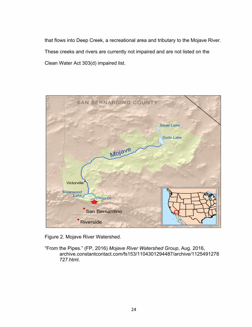
24

that flows into Deep Creek, a recreational area and tributary to the Mojave River.

These creeks and rivers are currently not impaired and are not listed on the

Clean Water Act 303(d) impaired list.

Figure 2. Mojave River Watershed.

“From the Pipes.” (FP, 2016) Mojave River Watershed Group, Aug. 2016, archive.constantcontact.com/fs153/1104301294487/archive/1125491278 727.html.

25

In 2016, the NRCS contributed to the restoration and BMPs of Hencks

Meadow. The BMPs included three water and sediment control basins connected

by four lined waterways or outlets to the existing man-made pond. The drainage

area into the site location is forest cover, green space (e.g. meadow, biking trails,

and hiking trails), and impervious surfaces (e.g. park, parking lot, and highway).

The water testing sites consists of the three BMP water detention basins and the

existing man-made pond. The first basin is Pond 1 located at the drainage of the

parking lot, the second is basin Pond 2, the third basin is Pond 3, and the

existing man-made pond is Pond 4. The site elevation is 5,660 to 5,730 ft (McGill,

2017). Hencks Meadow has a downhill 25-35 ft. gradient from Pond 1 to Pond 4.

Skypark is 233.76 acres within a hydrologic catchment area of 1,200.57 acres,

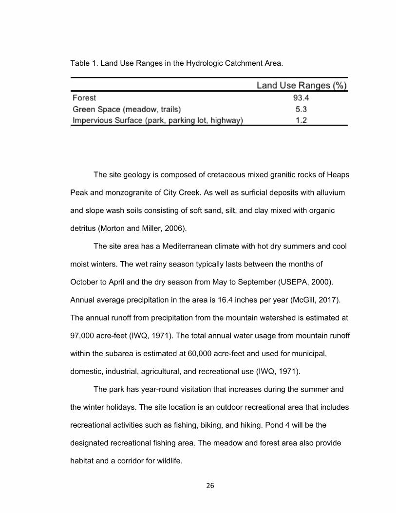
including 1,121.85 acres of forest cover. The land use includes forest cover

(93.4%), green space (5.3%), and impervious surfaces (1.2%), see Table 1. The

green space is a combination of natural pervious areas with recreational uses

including the meadow (3.7 acres), and hiking and biking trails (60.02 acres). The

impervious surfaces include 7.3 acres of the park (e.g. rooftops and pathways), a

2.42-acre parking lot, and 5.28 acres of the surrounding highway (Skypark,

2017).

26

Table 1. Land Use Ranges in the Hydrologic Catchment Area.

The site geology is composed of cretaceous mixed granitic rocks of Heaps

Peak and monzogranite of City Creek. As well as surficial deposits with alluvium

and slope wash soils consisting of soft sand, silt, and clay mixed with organic

detritus (Morton and Miller, 2006).

The site area has a Mediterranean climate with hot dry summers and cool

moist winters. The wet rainy season typically lasts between the months of

October to April and the dry season from May to September (USEPA, 2000).

Annual average precipitation in the area is 16.4 inches per year (McGill, 2017).

The annual runoff from precipitation from the mountain watershed is estimated at

97,000 acre-feet (IWQ, 1971). The total annual water usage from mountain runoff

within the subarea is estimated at 60,000 acre-feet and used for municipal,

domestic, industrial, agricultural, and recreational use (IWQ, 1971).

The park has year-round visitation that increases during the summer and

the winter holidays. The site location is an outdoor recreational area that includes

recreational activities such as fishing, biking, and hiking. Pond 4 will be the

designated recreational fishing area. The meadow and forest area also provide

habitat and a corridor for wildlife.

27

The original Santa’s Village amusement park was open from 1955 to

1998. While the park was closed, the Old Fire in 2003 burned vegetation on the

property, clearing trees and shrubs west of the parking lot. Also, from 2004 to

2013, the parking lot and meadow area was used as a dumping ground for

infected bark beetle trees.

28

CHAPTER THREE

METHODS

Water Quality Testing

The NRCS designed and constructed impoundments forming a series of

BMP water and sediment control basins, conservation practice standard code

638, interconnected by four lined waterways or outlets, conservation practice

standard code 468 displayed in Figure 3. BMP installation and construction

occurred throughout 2016 and 2017. Water and sediment control basins detain

and capture stormwater runoff, trap sediment, reduce erosion, and improves

downstream water quality. The first water and sediment control basin is Pond 1,

which is 321 cu. yd., 45 by 75 ft., and 5-6 ft. deep. The second basin is Pond 2,

at 713 cu. yd., 68 by 80 ft., and 6-7 ft. deep. The third basin is Pond 3, sized at

849 cu. yd., 71 by 93 ft., and 7-8 ft. deep, and Pond 4 is the existing man-made

pond. The lined waterways are designed with rock riprap and geotextile fabric to

reduce erosion, improve water quality, and provide safe conveyance of

stormwater runoff. All waterways are 10 ft. wide and 2 ft. deep, with an additional

1-1.5 ft. depth of rocks. The length of the first lined waterway is 55 ft., draining

the parking lot into Pond 1. The second waterway is 481 ft., separated by a

vegetated area, draining Pond 1 to Pond 2. The third waterway is 190 ft., draining

Pond 2 to Pond 3 and the fourth is 105 ft., draining from Pond 3 to Pond 4

(Skypark, 2017). The basins collect stormwater runoff from impervious surfaces

and forest cover. Runoff from the parking lot, highway, and park drain directly

29

into Pond 1. When rainfall exceeds the depth of each pond, the captured

stormwater runoff overflows into the next pond via the waterways. When

stormwater exceeds Pond 4, it overflows into the surface water stream Hooks

Creek.

Figure 3. NRCS Constructed Sediment Basins and Waterways.

Skypark Revised Final EIR Appendices 2017 (Skypark, 2017). http://cms.sbcounty.gov/lus/Planning/Environmental/Mountain.aspx (assessed March 3, 2018), San Bernardino County Land Use Services.

30

Water quality samples of the BMP detention basins were collected to

determine the effectiveness of these mitigation practices from impervious surface

stormwater runoff. The water quality was sampled during an eight-month period

from January 2018 through August 2018 to determine baseline conditions,

effectiveness of BMPs, and to compare results to water quality criteria and

objectives. Each water quality parameter was analyzed separately for each pond.

The water quality testing events were divided seasonally, spring and summer to

indicate trends based on seasonality. Spring consisted of February through mid-

May and summer consisted of mid-May through mid-August. Four sites were

selected, one sampling site for each pond. Sampling locations for Pond 1

occurred at the north side, while on the east side of Ponds 2 and 3, and on the

southwest side of Pond 4. Water testing was shore side at surface water depths

of 1-6 inches except Pond 4, which was tested on a 20 ft dock. Sites were

assessed with the permission of the private owner. Seven water quality

parameters were measured in situ biweekly and monthly grab samples for six

water quality parameters were transported to California State University, San

Bernardino laboratory for analysis. In situ water testing ranged from March

through August due to equipment availability, including 14 biweekly sampling

events. Laboratory testing ranged from January through August, including 8

monthly sampling events. Water testing and sample collection variability was

reduced by consistent sampling location and proper methods at a consistent

morning time regime (i.e. 8am-12pm).

31

Sampling Procedures

Water temperature (ºC)(Temp), dissolved oxygen (mg/L)(DO), pH,

turbidity (NTU)(Turb), conductivity (µS/cm)(Cond), nitrate (mg/L)(NO3-), and

ammonium (mg/L)(NH4+) were measured in situ with a Vernier LabQuest 2

instrument. The probes included the Extra Long Temperature Probe, the Vernier

Optical DO Probe, and the pH Sensor, calibrated with pH buffer solution. The

Conductivity Probe was used and calibrated with a Sodium Chloride Solution

Conductivity Standard, 500 (mg/L) total dissolved solids, 1000 (µS/cm). The

Nitrate Ion-Selective Electrode Probe was used and calibrated with a Sodium

Nitrate Standard of 1 (ppm) and 100 (ppm) NO3- as N. The Ammonium Ion-

Selective Electrode Probe was used and calibrated with an Ammonium Chloride

Standard of 1 (ppm) and 100 (ppm) NH4+ as N. The Turbidity Sensor is a light

scattering method that requires a water sample collection that is placed inside

the sensor and recorded. The turbidity sensor was calibrated using the StablCal

Formazin Standard 10 (NTU) and 100 (NTU) (LQ2, 2018).

Water quality parameters for the grab samples and analysis in the lab

included total suspended solids (mg/L)(TSS), total dissolved solids (mg/L)(TDS),

chemical oxygen demand (mg/L)(COD), total coliform (MPN/100mL)(TC),

Escherichia coli (MPN/100mL)(E. coli), and trace metals (µg/L). The grab

samples for TSS, TDS, COD, and trace metals were collected in 1 (L) brown

opaque HDPE plastic bottles that were acid washed using EPA protocols. The

acid wash included a wash with trace metal phosphate free laboratory detergent,

rinsed with tap water, then washed with 50:50 HNO3 and deionized (DI) water,

32

and rinsed with DI water. Samples were kept on ice, in a cooler and refrigerated

in the lab at 4 (°C) until analyzed.

Total suspended solids included 27 samples that were examined using

Standard Methods 2540 D, using the approved 47 (mL) pure glass fiber filters

(APHA, 2005). Total dissolved solids included 27 samples that were assessed

using Standard Methods 2540 B (APHA, 2005). Chemical oxygen demand

included 27 samples that were analyzed using the HACH digestion vials, low

range 3-150 (mg/L), under the USEPA Reactor Digestion Method 8000, which is

equivalent to Standard Methods 5220 C (APHA, 2005). The calibration curve was

prepared according to Standard Methods using phthalate potassium hydrate

(APHA, 2005). Both calibration standards and samples were analyzed using a

Thermo Aquamate visible spectrometer with absorbance values read at 420

(nm).

In this study, there were 17 samples of total coliform and 17 samples of E.

coli collected and analyzed. Bacteria samples were collected biweekly in 100

(mL) sealed sterile plastic bottles. Samples were kept on ice, in a cooler, and

processed in the laboratory within 6 hours of collection. Total coliform and E. coli

were analyzed using U.S. EPA approved IDEXX methods, Colilert-18, Colisure,

and Quanti-Tray/2000 (USEPA, 2003). Results were reported as most probable

number per 100mL (MPN/100mL) of water. Bacteria testing began in mid-May

due to equipment availability.

During the study, two testing events with 8 total samples for trace metals

were analyzed. Trace metals were analyzed for total recoverable metals under

33

EPA method 200.8 (USEPA, 1994). The digested water samples were analyzed

by PHYSIS Environmental Laboratories, Inc. (PHYSIS) for total trace metals by

EPA 200.8. The trace metals included were Aluminum (Al), Antimony (Sb),

Arsenic (As), Barium (Ba), Beryllium (Be), Cadmium (Cd), Chromium (Cr), Cobalt

(Co), Copper (Cu), Iron (Fe), Lead (Pb), Manganese (Mn), Molybdenum (Mo),

Nickel (Ni), Selenium (Se), Silver (Ag), Strontium (Sr), Thallium (Tl), Tin (Sn),

Titanium (Ti), Vanadium (V), and Zinc (Zn). The trace metals analyzed for this

study are subsets of these metals including As, Cd, Cr, Co, Cu, Pb, Mn, Ni, Ag,

and Zn that are toxic and more of a concern in the environment.

Data Analysis

The results of the study were compared to the U.S. EPA Recreational

Water Quality Criteria for bacteria and to the objectives from the State of

California, State Water Resources Control Board, South Lahontan Region for

DO, pH, nitrate, and TSS (USEPA, 2012; WQCP, 2015). The results of trace

metals have been compared to the U.S. EPA National Recommended Water

Quality Criteria - Aquatic Life Criteria (USEPA). Descriptive statistics using

Microsoft Excel 2018 and SPSS were performed including the mean, standard

deviation, variance, and minimum/maximum for each pond and parameter.

These methods and analysis are similar to Barakat et al. (2016), Cahoon et al.

(2006), Ensign and Mallin (2001), Mallin et al. (2016), Schoonover et al. (2005),

and Schreiber et al. (2003).

Watershed land use was determined using satellite imagery from Google

Earth and Google Earth WATERSKMZ Tool providing geospatial WATERS data

34

(USEPA, 2017). Daily precipitation data during this period was acquired from

Weather Underground, Skyforest, California (SWU, 2018).

35

CHAPTER FOUR

RESULTS

The U.S. EPA Recreational Water Quality Criteria and the State of

California, State Water Resources Control Board, South Lahontan Region

Objectives, and San Bernardino Mountains Hooks Creek Objectives are

displayed in Table 2 (USEPA, 2012; WQCP, 2015). When EPA standards are not

developed for a given water quality metric under observation for this study

period, the Lahontan Region and Hooks Creek Objectives were included as an

alternative criteria tool. Individual samplings and water quality metric means were

both assessed to determine if they meet the listed criteria and recommendations

since means can mask episodic sampling events that may not meet EPA criteria,

regional and local objectives.

It should be noted not all water quality parameters have a set standard or

objective and some metrics were only tested a few times including total coliform,

E. coli, TSS, TDS, COD, and trace metals due to study funding limitations.

36

Table 2. Water Quality Criteria and Objectives.

The descriptive statistics for Pond 1, recommended water quality

criteria/objectives, and the number of testing events exceeding the standards are

indicated in Table 3 (USEPA, 2012; WQCP, 2015). Although the mean pH does

not exceed the Lahontan Region Objectives (6.5-8.5 - Table 2) during the study

period, four sampling events do not meet the objectives, including two events in

April (9.1 and 9.16), May (9.69), and June (8.63 - see Figure 7). Mean nitrate

levels do not exceed the Hooks Creek Objectives (0.8-2.5 mg/L - Table 2),

however, two sampling events do not meet the standard during April (0.7 mg/L

and 8.0 mg/L - reference Figure 10). Mean E. coli observations exceed the EPA

Recreational Criteria (<126 cfu/100mL - Table 2), however, only one testing

event in June (2419.6 MPN/100mL - see Figure 16) did not meet the standard.

Lastly, the mean TDS meets the Hooks Creek Objectives (<127 mg/L - Table 2)

with only two sampling events exceeding the objectives in January (146 mg/L)

and June (164 mg/L - see Figure 13 below).

37

Table 3. Pond 1 Descriptive Statistics and Exceedances.

Table 4 illustrates descriptive statistics for Pond 2, water quality

criteria/objectives, and the amount of times each metric exceeded the

recommended standard (USEPA, 2012; WQCP, 2015). Although the mean DO

meet the Lahontan Region Objectives (>4 mg/L - Table 2), one testing event in

July (3.55 mg/L - Figure 6) did not meet the objective. Mean pH does not exceed

the Lahontan Region Objectives (Table 2), however, one testing event in April

(8.9 - Figure 7) exceeded the objective. On average, nitrate levels do not exceed

the Hooks Creek Objectives (Table 2), however, when observing individual

sampling events, two testing events in July (7.1 mg/L and 3.2 mg/L), and one in

August (6.9 mg/L - Figure 10) did not meet the objectives. When considering

bacterial characteristics of Pond 2, both the mean and a majority of sampling

events meet the EPA E. coli standards (Table 2). In June, only one event

exceeded the standard (191.8 MPN/100mL - see Figure 16 below). This trend is

38

also replicated when observing trends in TDS where the average did not exceed

the Hooks Creek Objectives (Table 2). Although, one event in August (270 mg/L -

Figure 13) exceeded the objective.

Table 4. Pond 2 Descriptive Statistics and Exceedances.

Descriptive statistics for samples taken from Pond 3 during the study

period, water quality criteria/objectives, and the number of events exceeding the

guidelines are displayed in Table 5 (USEPA, 2012; WQCP, 2015). Most of the

water quality metrics means and individual samples meet the standards and

objectives with the exception of pH and nitrate. Mean pH levels meet the

standard (Table 2) for samples taken during the study period with only one

sample exceeding in April (8.77 - see Figure 7). The mean nitrate levels do not

39

exceed the standard (Table 2), however, one event in July (0.4 mg/L - Figure 10)

was below the standard level.

Table 5. Pond 3 Descriptive Statistics and Exceedances.

Table 6 illustrates the descriptive statistics for Pond 4 for each water

quality metric observed, water quality criteria/objectives, and the number of

events exceeding the recommended standards (USEPA, 2012; WQCP, 2015).

The mean pH does not exceed the standard (Table 2), although, four test events

do not meet the standard; June (9.4 and 9.64), July (9.69), and August (9.27 -

reference Figure 7). The mean nitrate levels do not exceed the standard (Table

2), however, 5 testing events including March (0.5 mg/L), April (0.4 mg/L and 0.7

mg/L), May (0.7 mg/L), and August (3.0 mg/L - Figure 10 below) do not meet the

standard.

40

Table 6. Pond 4 Descriptive Statistics and Exceedances.

The U.S. EPA National Recommended Water Quality Criteria, Aquatic Life

Criteria, including acute and chronic standards for trace metals, and the minimum

and maximum of two testing events is indicated in Table 7 (USEPA). Total

chromium measurements were taken in March, although, EPA Aquatic Criteria

are designated for chromium (III) and chromium (VI). The total chromium levels

do not meet the chromium (VI) EPA acute standard (16 µg/L) three out of four

samples and do not meet the chronic standard (11 µg/L) for all four samples,

ranging from (12.6 µg/L and 57.1 µg/L - Figure 17). Lead results do not meet the

EPA chronic standard (2.5 µg/L) for all four samples during the March testing

event, ranging from (18.2 µg/L and 43.5 µg/L - Figure 18). Results for arsenic,

cadmium, chromium (III), nickel, silver, and zinc were below the acute and

chronic EPA Aquatic Life Criteria throughout the study (see - Appendix A).

41

Table 7. EPA Aquatic Life Criteria for Trace Metals.

Figure 4 indicates the daily total precipitation throughout the sampling

period, acquired from Weather Underground, Skyforest, California (SWU, 2018).

42

Figure 4. Daily Total Precipitation (In.).

The column graphs below compare water quality metrics for each pond

over time to determine the general trends. Graphs that contain any missing data

throughout the period are displaying equipment malfunctions. During the testing

period, Pond 1, 2, and 3 dried, therefore, graphs with missing data later on in the

study are due to low or no precipitation. The last testing event for Pond 1

occurred June 26th, Pond 3 July 10th, and Pond 2 August 7th.

Throughout the study period, the water temperature varied from 6.5 (°C) in

the spring and increased to 33.7 (°C) in the summer, see Figure 5. The maximum

temperatures occurred in Pond 1 (June 26th) and Pond 4 (June 12th) and the

43

minimum temperatures in Pond 2 and Pond 3 (April 17th). Dissolved oxygen

levels shown in Figure 6 during the study period, indicate that DO varied between

a minimum 3.55 (mg/L) in Pond 2 (July 24th) and a maximum 15.75 (mg/L) in

Pond 4 (June 26th). Trends indicate high levels of DO were maintained

throughout the spring and dropped during the summer. Throughout the study, pH

levels indicated in Figure 7 ranged from 6.45 and 9.69 and did not vary

seasonally. The pH levels for Pond 1 and Pond 4 were basic and Pond 2 and

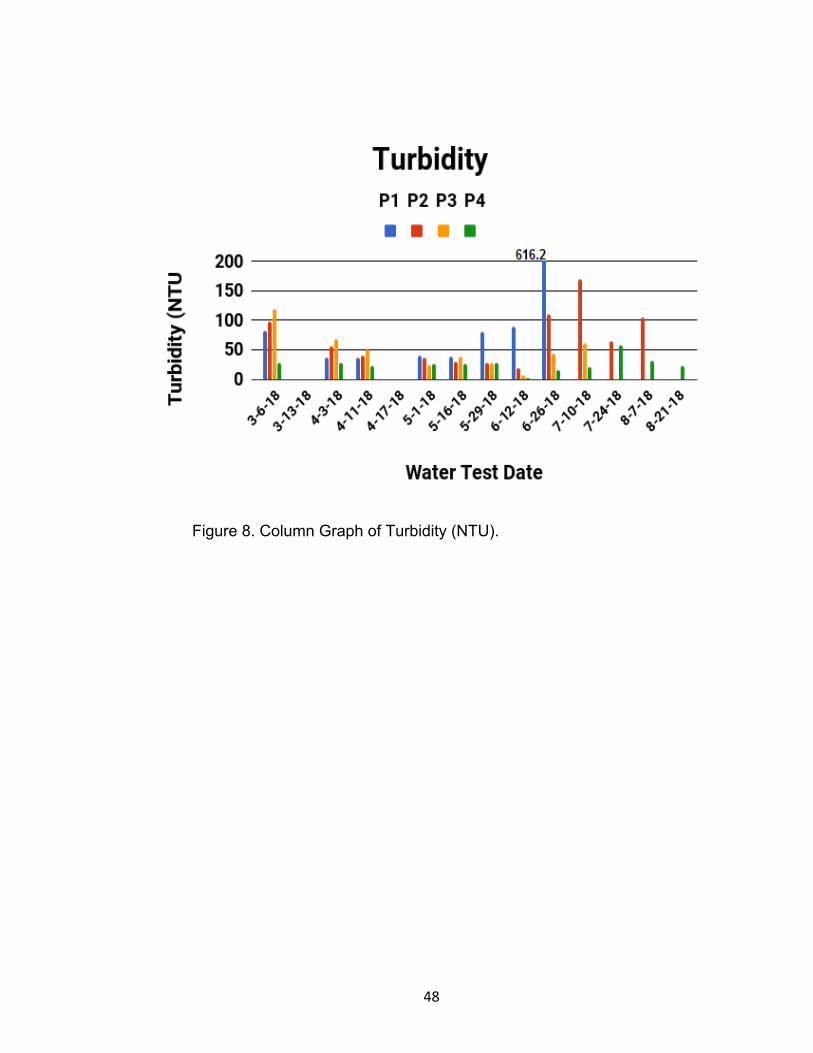
Pond 3 were neutral. Turbidity levels displayed in Figure 8 throughout the testing

period, fluctuated between 1.5 (NTU) and 169.8 (NTU), including an outlier for

Pond 1 at 616.2 (NTU) (June 26th). Turbidity trends indicate low levels in the

spring and high levels in the summer. Conductivity measurements ranged

between 63.5 (µS/cm) and 470 (µS/cm) with lower levels during the spring and

higher levels during the summer in Figure 9. Throughout the study, nitrate levels

as seen in Figure 10 fluctuate from 0.4 (mg/L) and 8.0 (mg/L). High levels of

nitrate are evident (April 17th) Pond 1 8.0 (mg/L) and Pond 2 (July 10th) 6.9

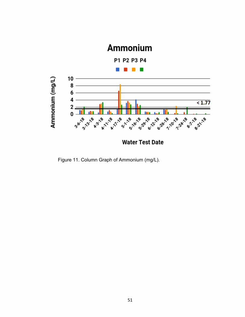
(mg/L) and (August 7th) 7.1 (mg/L). Ammonium concentrations shown in Figure

11 varied between 0.1 (mg/L) and 8.5 (mg/L). High levels of ammonium occur

during the spring (April 17th) for Pond 2 6.6 (mg/L) and Pond 3 8.5 (mg/L). Figure

12 shows total suspended solids levels for monthly events throughout the study

ranged between 1.3 (mg/L) and 149 (mg/L), with high levels during the spring.

Although, TSS levels were extremely high for Pond 1 149 (mg/L) (June 26th) and

Pond 2 54.5 (mg/L) (July 26th) during the summer, which may have been due to

low water levels. Total dissolved solids ranged from 8 (mg/L) and 270 (mg/L)

44

indicated in Figure 13. High results of TDS occur before water depletion of Pond

1 (June 26th) and Pond 2 (July 26th). Chemical oxygen demand levels shown in

Figure 14 ranged from 0.3 (mg/L) and 157.2 (mg/L), with low levels during the

spring and high levels during the summer. Indicated in Figure 15, total coliform

concentrations were high for all ponds throughout sampling, ranging between 4.1

(MPN/100mL) and >2419.6 (MPN/100mL). E. coli concentrations shown in Figure

16 ranged from <1 (MPN/100mL) and 2419.6 (MPN/100mL). E. coli for Pond 1

was extremely high before depletion (June 26th), reaching 2419.6 (MPN/100mL)

and Pond 2 had high levels as well during the same testing event. Figure 17

shows chromium and Figure 18 shows lead concentrations were high during the

second testing event (March 8th). Chromium levels varied from 0.732 (µg/L) and

57.1 (µg/L) and lead varied between 0.362 (µg/L) and 43.5 (µg/L).

45

Figure 5. Column Graph of Water Temperature (°C).

46

Figure 6. Column Graph of Dissolved Oxygen (mg/L).

47

Figure 7. Column Graph of pH.

48

Figure 8. Column Graph of Turbidity (NTU).

49

Figure 9. Column Graph of Conductivity (µS/cm).

50

Figure 10. Column Graph of Nitrate (mg/L).

51

Figure 11. Column Graph of Ammonium (mg/L).

52

Figure 12. Column Graph of Total Suspended Solids (mg/L).

53

Figure 13. Column Graph of Total Dissolved Solids (mg/L).

54

Figure 14. Column Graph of Chemical Oxygen Demand (mg/L).

55

Figure 15. Column Graph of Total Coliform (MPN/100mL).

56

Figure 16. Column Graph of E. coli (MPN/100mL).

57

Figure 17. Column Graph of Chromium (µg/L).

58

Figure 18. Column Graph of Lead (µg/L).

59

CHAPTER FIVE

DISCUSSION

Water Quality Parameters

The BMP design has shown to be effective overall at improving

impervious surface stormwater runoff throughout the detention pond system and

before entering Hooks Creek. Overall, the ponds are meeting the U.S. EPA

Water Quality Criteria and the State of California, Lahontan Region Water Quality

Objectives. The ponds are improving downstream surface water quality by

capturing and storing runoff instead of allowing direct inputs into stream surface

water. The results from this study indicate that pollutants are collecting on

impervious surfaces (e.g. park, parking lot, and highway) and are being

transported via stormwater runoff into Pond 1. As expected, Pond 1 has the

highest pollutant concentrations since it receives the direct discharge from

impervious surfaces. During the testing period, the concentration of pollutants

decreased from Pond 1 to Pond 4. The sequence of ponds acted as a natural

storage area and cleansing system allowing filtration and settling of pollutants.

Throughout the study, a baseline of water quality parameters and trends was

determined. The study also indicates trends of precipitation and water quality

during rain events, wet vs. dry periods. During wet periods, pollutant

concentrations were higher due to rainfall creating stormwater runoff inputs and

transport of pollutants. Dry periods allowed water storage, infiltration, settling,

and evaporation.

60

Water Temperature

Water temperature alterations impact water quality by increasing plant and

algae growth and decreasing aquatic health causing stress and lower resistance

to pollutants (LQ2, 2018). The water temperature varied due to seasonal

variability with cooler temperatures during the spring and warmer temperatures

during the summer, as observed in Barakat et al. (2016), Kazi et al. (2009), and

Vega et al. (1998). According to the literature, multiple studies including Binkley

and Brown (1993) and Corbett et al. (1978) have observed that water

temperature is directly related to sunlight exposure and tree cover. Observations

throughout the study indicate that temperature fluctuations between ponds may

be due to these natural environmental impacts. During testing events, Pond 1

was in direct sunlight, Pond 2 and Pond 3 were shaded by tree cover, and Pond

4 was partially shaded. There is missing data in Figure 5 (March 6th) due to

equipment error. Pond 1 was dry on July 10th, Pond 3 was dry by July 24th, and

Pond 2 on August 21st.

Dissolved Oxygen

Dissolved oxygen is a very important indicator of water quality and the

protection of aquatic life because it can reduce aquatic diversity and cause fish

kills. Fluctuations of DO levels are impacted by temperature, plant and algae

growth, and decaying organic matter (LQ2, 2018). Dissolved oxygen indicated

seasonal variability with low levels during the summer months July and August,

as seen in Yang et al. (2007) due to warmer temperatures and microorganism

activity. Seasonal trends in this study during the spring indicate cold

61

temperatures and high levels of DO, while the summer has warm temperatures

with low levels of DO. These results relate to the literature including Barakat et al.

(2016), Kumari et al. (2013), Varol et al. (2012), and Vega et al. (1998) that

observed relationships between DO and temperature, indicating colder water

increases oxygenation, therefore increases DO levels. It must be noted that

water reduced over time, which could also be driving these trends. Possible high

levels of DO during testing may have been caused by nutrient inputs and algae

production from photosynthesis. When algae deplete, DO levels decrease due to

aerobic organisms breaking down and decomposing organic matter and

consuming all of the oxygen as indicated in Vega et al. (1998) and Yang et al.

(2007). Although algae was not measured, there were observations of algae

growth in Pond 1 from mid-April to mid-May and high levels of DO, which may

have been promoted by high levels of nutrients (April 17th) (Burkholder et al.,

2007). During the end of May, Pond 1 had no algae growth, low levels of

nutrients, and low levels of DO. Algae depletion may have been due to the dry

period, because the pond was no longer receiving nutrients from rain runoff. The

results and observations of Pond 4 also indicate algae growth and mild

eutrophication. Seasonal trends show that during the warmer summer months,

algal blooms were observed the end of July and August, and the DO levels

began to drastically decrease. These fluctuations can potentially create a toxic

system for sensitive aquatic species. There is no DO data on July 10th Figure 6,

due to equipment error. Pond 1 is dry starting July 10th, Pond 3 as of July 24th,

and Pond 2 on August 21st.

62

pH

The fluctuation of pH levels creates toxic environments that impact plant

and aquatic health and cause decreases in survival and reproduction (LQ2,

2018; Yang et al., 2007). Pond 1 results indicate strong basic levels, also

observed in Khatoon et al. (2013) and Yang et al. (2007) since surface waters

are naturally more basic. Although for this site location, trends may be due to

direct runoff and leaching from basic cement material. However, there are also

trends of acidic levels after rain events in March and May. These results are

expected because rain has more acidic levels ranging from 5.5-6 (LQ2, 2018).

There is no clear reason for basic pH levels in Pond 4, however, it may be due to

natural erosion of limestone deposits in soil containing bicarbonate and reacting

with runoff (LQ2, 2018). The results for pH do not show any trends related to

other water quality parameters throughout the study, also observed in Vega et al.

(1998). There is no data on March 13th and April 3rd Figure 7 due to equipment

malfunction. Pond 1 is dry on July 10th, Pond 3 is dry on July 24th, and Pond 2 is

dry on August 21st.

Turbidity

Turbidity determines the clarity by measuring the amount of light reflected

off particles in the water column. Low turbidity levels indicate low levels of

suspended solids and clear water. Turbidity fluctuates due to natural causes

including rain, runoff, sediment, and soil erosion. Turbidity impacts aquatic plants

and animals and high levels can reduce photosynthesis rates. Turbidity impacts

other water quality parameters including increases in temperature and decreases

63

in DO. Turbidity also impacts recreation and can make a body of water

aesthetically not pleasing. Seasonal trends of high turbidity levels for Pond 1 and

Pond 2 during the summer may be due to shallow pond depths from evaporation

and infiltration. Pond 1 results indicate high levels at 616.2 (NTU) at the end of

June before the pond was depleted of water. According to Barakat et al. (2016),

there are positive trends between turbidity, TSS, and ammonium, which can be

from materials in the water due to runoff during storm events. Throughout the

study, seasonal trends of high turbidity are indicated on March 6th for Ponds 1, 2,

and 3, which may be due to rain events from (February 24th to March 5th).

Although trends between turbidity and TSS were observed, no trends were

evident with ammonium. No data was recorded on (March 13th) and (April 17th)

Figure 8 due to equipment malfunction. Testing on July 10th Pond 1 is dry, July

24th Pond 3, and August 21st Pond 2.

Conductivity

Conductivity measures the electrical conductance of the water and

determines the amount of salinity. Conductivity can impact aquatic health when

freshwater ecosystems become too saline. Natural sources of soluble salts are

from rocks and soils, while inputs from human activities are fertilizers, salted

roads to melt ice and snow, and organic matter from wastewater treatment plants

(LQ2, 2018). Pond 1 may have higher conductance levels in April due to the

proximity and direct runoff from the salted highway and parking lot during and

after storm events from (March 10th to March 25th). Khatoon et al. (2013) and

Vega et al. (1998) indicated positive trends between conductivity and TDS, since

64

both parameters measure the amount of dissolved salt. Throughout this study,

conductivity and TDS show seasonal trends of low levels during the spring and

high levels during the summer. In Figure 9, Pond 1 is dry during testing on July

10th, July 24th for Pond 3, and August 21st for Pond 2.

Nitrate

Nitrate is a form of nitrogen naturally found in the environment from air

deposition, animal waste, and plant and animal decomposition that can

accumulate in soils, surface water, and groundwater (LQ2, 2018; Vitousek et al.,

1997). Excess nitrate levels may be due to human activities including wastewater

systems, fertilizer use, and animal waste that can lead to eutrophic conditions

and impact aquatic health (LQ2, 2018). Throughout the study, seasonal

variability indicates high nitrate levels during the summer months of July and

August and high events in the spring, which may be due to fertilizer use. Mallin et

al. (2000) observes trends of nitrate and E. coli, which may come from the same

source including sewage, animal waste, and fertilizer runoff. However, the trends

cannot be determined between nitrate and E. coli for this study due to irregular

testing events for bacteria. Figure 10 indicates that Pond 1 is dry by July 10th,

Pond 3 by July 24th, and Pond 2 by August 21st.

Ammonium

Ammonium is a form of nitrogen that is directly toxic to aquatic organisms

and can cause increases in plant and algae growth. Human sources are from

agricultural runoff, sewage treatment effluent, and industrial waste (LQ2, 2018).

Throughout the study, seasonal trends of high levels during the spring (April and

65

May) may be due to human activities, such as fertilizer use. Testing on July 10th

Pond 1 is dry, July 24th Pond 3, and August 21st Pond 2 in Figure 11.

Total Suspended Solids

Total suspended solids measure the clarity and the amount of particles in

the water column. Total suspended solids include silt, sediment, and decaying

organic matter that can impact stream health and aquatic life by blocking sunlight

for proper aquatic growth and interfere with fish gills (LQ2, 2018). According to

the literature, Barakat et al. (2016) indicated trends between turbidity and TSS,

as expected since both metrics measure the amount of particles in the water.

Trends throughout this study are evident between turbidity and TSS. Chen and

Chang (2014) observed trends between TSS and precipitation due to sediment

and topsoil in runoff. For this study, seasonal trends in spring indicate high TSS

levels on (March 6th and 23rd), which may be due to rain events from (February

24th to March 5th) and (March 10th to March 25th). Rainfall and runoff during

these wet periods may have created water mixture and increased sediment

inputs into the ponds. The high TSS results on June 26th for Pond 1 may be due

to low levels of water. Testing events on July 26th and August 21st have limited

data due to dry ponds shown in Figure 12.

Total Dissolved Solids

Total dissolved solids measure the amount of soluble salts in the water.

Total dissolved solids cause pH fluctuations and can impact aquatic health (LQ2,

2018). Pond 1 and Pond 3 are dry by August 26th and Pond 2 by August 21st,

displayed in Figure 13. It must be noted, that the Hooks Creek Objectives

66

standard for TDS is <127 (mg/L) for 90% of the time. These individual sampling

events meet the objective of 90% of the time.

Chemical Oxygen Demand

Chemical Oxygen Demand is the measure of oxidizable organic matter.

During this study, seasonal variability indicates high levels of COD during the

summer, as observed in Kumari et al. (2013) due to active microorganisms. Vega

et al. (1998) indicates negative trends with COD and DO, as COD increases and

consumes oxygen, DO levels begin to decrease. Throughout this study, seasonal

trends appear during summer months between COD, DO, and water temperature

with high COD levels, low DO levels, and warm temperatures. In Figure 14, July

26th and August 21st have limited data due to dry ponds.

Total Coliform

Total coliform is the natural amount of total nonpathogenic bacteria within

a water system (LQ2, 2018). Bacteria testing began in May due to study funding

limitations. There is no data later in the testing period starting July 24th due to

dry ponds. Although, not evident in Figure 15 Pond 4 on July 26th is 1

(MPN/100mL). Pond 1 and Pond 3 are dry as of July 24th and Pond 2 on August

21st in Figure 15.

E. coli

E. coli is an indicator bacterium for possible waterborne pathogens from

the digestive tract of warm-blooded animals. Pathogenic bacteria can impact

human health and cause gastroenteritis and other waterborne diseases (LQ2,

2018). It must be noted that these are individual sampling events with results that

67

rarely exceed the 30-day interval geometric mean average EPA Criteria <126

(cfu/100mL). Literature has shown, including Chen and Chang (2014), Dwight et

al. (2002), and Heaney et al. (2015) that rainfall has been associated with fecal

indicator bacteria. These results are due to increased transport and moisture for

survival, however, was not indicated throughout this study. Although, it must be

noted that bacteria testing did not occur until the summer season with few storm

events. Seasonal variability of past literature including Heaney et al. (2015) and

Wilson et al. (2007) have shown that indicator bacteria in water has higher levels

during warmer summer months than compared to colder winter months. These

trends cannot be related to this study due to the testing period of spring and

summer. Although, seasonal differences of high E. coli concentrations during the

summer may be due to warmer temperatures contributing to higher growth and

survival rates, greater recreational activities, and less runoff washing out the

water system as observed in Chen and Chang (2014). Relationships between E.

coli, TSS, and turbidity have been observed in past literature including Chen and

Chang (2014) and Mallin et al. (2000) via transported particulate matter or

resuspended particles. Throughout the study in June and July for Pond 1 and

Pond 2, E. coli, TSS, and turbidity indicate positive trends, however, it must be

noted that water depths were shallow. For this study, the units used to determine

E. coli concentrations was the most probable number (MPN), while the EPA

Recreational Criteria uses colony forming units (cfu). For all practical purposes

both units can be used for data interchangeably. Colony forming units are more

conservative results that only account for the viable live E. coli bacteria, while

68

MPN is a statistical relationship that includes both viable and nonviable E. coli

bacteria. E. coli testing began in May, due to study funding limitations. The E. coli

for Pond 4 is 1 (MPN/100mL) during each testing event. Pond 1 is dry as of July

24th. E. coli for Pond 2 is 1 (MPN/100mL) for May 21st and June 12th, and dry

on August 21st. The E. coli for Pond 3 on July 26th is 1 (MPN/100mL) and dry by

July 24th as shown in Figure 16.

Trace Metals

Trace metals can be toxic and impact human and aquatic health. Trace

metals were tested for two events in February and March due to the lack of study

funding and equipment limitations. Trace metals were not compared seasonally

or with other water metrics due to the limited testing events. Chromium and lead

are shown in Figure 17 and 18 because they did not meet the EPA Aquatic Life

Criteria. It must be noted that these results were only from one testing event and

were not replicated for further analysis. Also, total chromium levels cannot be

directly compared to EPA Aquatic Life Criteria because the criteria are for

chromium (III) and chromium (VI).

69

CHAPTER SIX

CONCLUSIONS

Water quality and quantity is important because it is essential for human

consumption and to sustain life. Current research has shown that water quality

and quantity is impacted by population growth, land types, and anthropogenic

activities creating nonpoint source pollution entering water resources. BMP

research has shown to reduce these adverse impacts by reducing stormwater

pollutants and improving water quality regionally and globally. Also, BMP

effectiveness is site specific depending on the site location, climate, watershed

size, surrounding land type, and pollutant concentrations. Although, BMPs have

shown to be successful, some BMPs have shown to be insufficient.

The primary goals of this research were to collect a baseline of water

quality parameters and to determine if the BMP design was effective. The

research demonstrates that the assessment of BMP performance was effective

for the site location, locally and regionally. Based on this study, the results

indicate that the BMP design will improve water quality and quantity in the

headwaters of the Mojave River Watershed. The results of the detention basins

are consistent with water quality improvement and BMP effectiveness in studies

such as Booth and Jackson (1997), Comings et al. (2000), and Piza et al. (2011).

The effectiveness of BMPs for this region can be directly related to other areas

with similar surface waters and can promote design and installation of BMPs.

Locally, the results of the study are paramount because the surface water leads

70

to a downstream recreational area and a growing community that needs pristine

water quality and quantity. The results are also important for this site location

because poor water quality can have negative impacts on the park’s tourism,

revenue, and reputation.

Overall, improvement of water quality protects public health, aquatic

ecosystems, and the environment. Applying this research model to other

locations may help elevate our understanding of the effectiveness of mitigation

practices to diminish impaired water quality. It should be noted that the study did

not account for natural and anthropogenic factors including groundwater,

evaporation, evapotranspiration, infiltration rates, and possible septic tank

leakage because it was beyond the scope of this study. The results and

knowledge obtained from this research suggest several avenues for future

research including applying BMPs to other site locations in the Southwestern

U.S. and may assist in continuous water quality monitoring. Recommendations

for future BMP research include a longer water quality testing period, consistent

testing events for all parameters, groundwater levels, and infiltration rates to

determine more consistent results and if surface water infiltration is impacting

groundwater quality. Future water quality challenges include increases in

population, urbanization, and climate change which can cause an increase of

impaired water resources. The continuation and effectiveness of BMPs is

essential to mitigate these harmful impacts and successfully improve water

quality and quantity on a global geographical scale for future generations.

71

APPENDIX A

TABLES

72

Table A1. Water Quality Parameters, Acronym, Analytical Method, and Units.

73

Table A2. Trace Metals.

74

Table A3. Trace Metals.

75

Table A4. Trace Metals.

76

Table A5. Trace Metals.

77

Table A6. Trace Metals.

78

Table A7. Trace Metals.

79

Table A8. Trace Metals.

80

Table A9. Trace Metals.

81

APPENDIX B

FIGURES

82

Figure B1. Displays the Interim Water Quality Control Plan California Regional Water Quality Control Board, South Lahontan Region 6B (IWQ, 1971).

83

Figure B2. Displays Hooks Creek Subunit, Hencks Meadow, and the Existing Man-Made Pond (Harder, 2016)

84

Figure B3. Hydrologic Catchment, Using U.S. EPA WATERS Data, Google Earth WATERSKMZ (USEPA, 2017).

85

Figure B4. USDA NRCS Soil Survey, Skypark (USDA, 2017).

86

Figure B5. Google Earth Image of Hencks Meadow (SS, 2017).

87

Figure B6. Pond 1, Inlet Waterway 1 from Parking Lot.

88

Figure B7. Pond 2, Waterway 2.

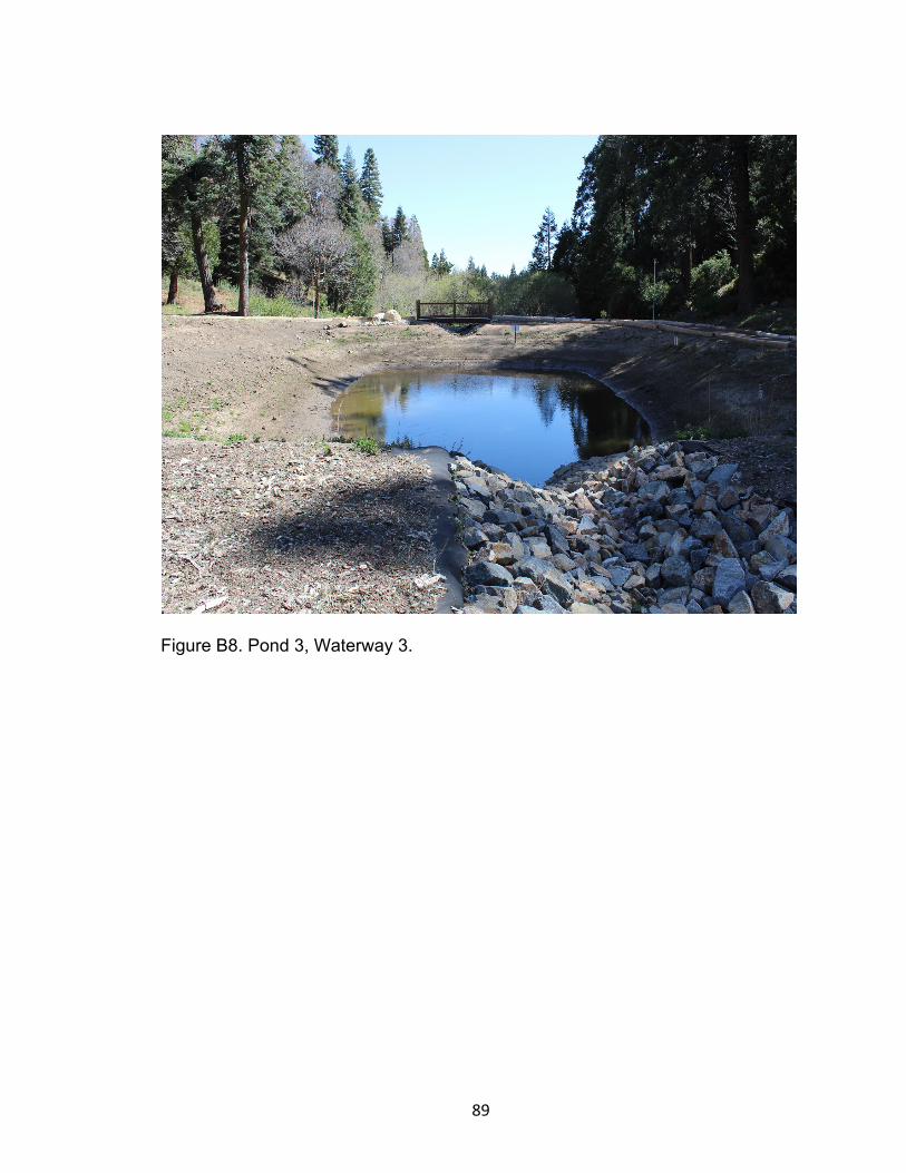
89

Figure B8. Pond 3, Waterway 3.

90

Figure B9. Pond 4, Waterway 4.

91

Figure B10. Column Graph of Arsenic Concentrations (µg/L) vs. Testing Event Dates, February 20, 2018 to March 8, 2018.

92

Figure B11. Column Graph of Cadmium Concentrations (µg/L) vs. throughout testing events.

93

Figure B12. Column Graph of Cobalt Concentrations (µg/L) vs. Testing Events.

94

Figure B13. Column Graph of Copper Concentrations (µg/L) vs. Testing Events.

95

Figure B14. Manganese Concentrations (µg/L) vs. Sampling Events.

96

Figure B15. Graph of Nickel Concentrations (µg/L) vs. Testing Events.

97

Figure B16. Silver Concentrations (µg/L) vs. Testing Events.

98

Figure B17. Column Graph of Zinc Concentrations (µg/L) vs. Two Testing Events.

99

REFERENCES

Alford, J. B.; Debbage, K. G.; Mallin, M. A.; Liu, Z. Surface Water Quality and Landscape Gradients in the North Carolina Cape Fear River Basin, The Key Role of Fecal Coliform. Southeastern Geographer, 2016, 56, 4, 428 453. APHA, AWWA, WEF 2005. Standard Methods for Examination of Water and Wastewater. American Public Health Association, Washington, DC. Arnold, C. L.; Gibbons, C. J. Impervious Surface Coverage: The Emergence of a Key Environmental Indicator. J. Am. Plann. Assoc. 1996, 62, 2, 243–258. Barakat, A.; Baghdadia, M. E.; Raisa, J.; Aghezzafb, B.; Slassib, M. Assessment of Spatial and Seasonal Water Quality Variation of Oum Er Rbia River (Morocco) Using Multivariate Statistical Techniques. ISWCR. 2016, 4, 284-292. Barret, M. E. Comparison of Structural Stormwater Best Management Practices. Water Environ. Res. 2005, 77, 1, 78-86. Billen, G.; Garnier, J.; Ficht, A.; Cun, C. Modeling the Response of Water Quality in the Seine River Estuary to Human Activity in its Watershed Over the Last 50 Years. Estuaries 2001, 24, 6B, 977-993.

Binkley, D.; Brown, T. C.; Forest Practices as Nonpoint Sources of Pollution in North America. Water Resour. Bull. 1993, 29, 5, 729-740. Booth, D. B.; Jackson, C. R. Urbanization of Aquatic Systems: Degradation Thresholds, Stormwater Detection, and the Limits of Mitigation. JAWRA. 1997, 33, 5, 1077-1090. Brabec, E.; Schulte, S.; Richards, P. L. Impervious Surfaces and Water Quality: A Review of Current Literature and Its Implications for Watershed Planning. JPL. 2002, 16, 4, 499-514. Braune, M. J.; Wood, A. Best Management Practices Applied to Urban Runoff Quantity and Quality Control. Wat. Sci. Tech. 1999, 39, 12, 117–121. Burkholder, J.; Libra, B.; Weyer, P.; Heathcote, S.; Kolpin, D.; Thorne, P. S.; Wichman, M. Impacts of Waste from Concentrated Animal Feeding Operations on Water Quality. Environ. Health Perspect. 2007, 115, 2, 308 312.

100

Burkholder, J. M.; Mallin, M. A.; Glasgow. Jr., H. B.; Larsen, L. M.; Mclver, M. R.; Shank, G. C.; Deamer-Melia, N.; Briley, D. S.; Springer, J.; Touchette, B. W.; Hannon, E. K. Impacts to a Coastal River and Estuary from Rupture of a Large Swine Waste Holding Lagoon. J. Environ. Qual. 1997, 26, 6, 1451-1466. Cahoon, L. B.; Hales, J. C.; Carey, E. S.; Loucaides, S.; Rowland, K. R.; Nearhoof, J. E. Shellfishing Closures in Southwest Brunswick County, North Carolina: Septic Tanks vs. Storm-Water Runoff as Fecal Coliform Sources. JCR. 2006, 22, 2, 319-327. Carpenter, S. R.; Caraco, N. F.; Correll, D. L.; Howarth, R. W.; Sharpley, A. N.; Smith, V. H. Nonpoint Pollution of Surface Waters with Phosphorus and Nitrogen. Ecological Applications 1998, 8, 3, 559-568. Chen, H. J.; Chang, H. Response of Discharge, TSS, and E. Coli to Rainfall Events in Urban, Suburban, and Rural Watersheds. Environ. Sci.-Proc Imp. 2014, 16, 2313-2324. Comings, K. J.; Booth, D. B.; Horner, R. R. Stormwater Pollutant Removal by Two Wet Ponds in Bellevue, Washington. 2000, 1-24. Corbett, E. S.; Lynch, J. A.; Sopper, W. E. Timber Harvesting Practices and Water Quality in the Eastern United States. J. Forest. 1978, 76, 8, 484 488. Corrao, M. V.; Cosens, B. E.; Heinse, R.; Eitel, J. U. H.; Link, T. E. Using Science to Bridge Management and Policy: Terracette Hydrologic Function and Water Quality Best Management Practices in Idaho. Rangelands 2015, 37, 5, 191-199. Dodds, W. K.; Oakes, R. M. Headwater Influences on Downstream Water Quality. Environ. Manage. 2007, 41, 367-377. Dwight, R. H.; Semenza, J. C; Baker, D. B.; Olsen, B. H. Association of Urban Runoff with Coastal Water Quality in Orange County, California. Water Environ. Res. 2002, 74, 82-90. Ellis, J. B.; Marsalek, J. Overview of Urban Drainage: Environmental Impacts and Concerns, Means of Mitigation and Implementation Policies. J. Hydraul. Res. 1996, 34, 6, 723-731. Ensign, S.H.; Mallin, M. A. Stream Water Quality Changes Following Timber Harvest in a Coastal Plain Swamp Forest. Wat. Res. 2001, 35, 14, 3381 3390.

101

“From the Pipes.” (FP, 2016) Mojave River Watershed Group, Aug. 2016, archive.constantcontact.com/fs153/1104301294487/archive/1125491278 727.html. Gautum, M. R.; Acharya, K.; Stone, M. Best Management Practices for Stormwater Management in the Desert Southwest. J. Contemp. Water Res. Educ. 2010, 146, 39-49. Genito, D.; Gburek, W. J.; Sharpley, A. N. Response of Stream Macroinvertebrates to Agricultural Land Cover in a Small Watershed. J. Freshwater Ecol. 2002, 17, 1, 109-119. Gleick, P. H. Water in Crisis: Paths to Sustainable Water Use. Ecol. Soc. Am. 1998, 571-579. Grimm, N. B.; Foster, D.; Groffman, P.; Grove, J. M.; Hopkinson, C. S.; Nadelhoffer, K. J.; Pataki, D. E.; Peters, D. P. C. The Changing Landscape: Ecosystem Responses to Urbanization and Pollution Across Climatic and Societal Gradients. Front. Ecol. Environ. 2008, 6, 5, 264-272. Harder, T. Hydrogeologic Evaluation of the Proposed Skypark at Santa's Village. Skypark at Santa's Village Technical Memorandum 8 Jan. 2016. Hathway, J. M.; Hunt, W. F.; Jadlocki, S. Indicator Bacteria Removal in Storm Water Best Management Practices in Charlotte, North Carolina. J. Environ. Eng. 2009, 125, 12, 1275-1285. Heaney, C D.; Myers, K.; Wing, S.; Hall, D.; Baron, D.; Stewart, J. R. Source Tracking Swine Fecal Waste in Surface Water Proximal to Swine Concentrated Animal Feeding Operations. Sci. Total Environ. 2015, 511, 676-683. Hicks, A. L.; Larson, J. S. Focus 2: Watershed Development Effects in Water Surplus Regions, The Impact of Urban Stormwater Runoff on Freshwater Wetlands and the Role of Aquatic Invertebrate Bioassessment. In Effects of Watershed Development and Management on Aquatic Ecosystems; Roesner, L. A., Eds.; ASCE: New York, 1997; pp 386-401. Holland, A. F.; Sanger, D. M.; Gawle, C. P.; Lerberg, S. B.; Santiago, M. S.; Riekerk, G. H. M.; Zimmerman, L. E.; Scott, G. I. Linkages Between Tidal Creek Ecosystems and the Landscape and Demographic Attributes of their Watersheds. J. Exp. Mar. Bio. Ecol. 2004, 298, 151-178.

102

Hooiveld, M.; Smit, L. A. M.; Beer, F. S.; Wouters, I. M.; Dijk, C. E.; Spreeuwenberg, P.; Heederik, D. J. J.; Yzermans, C. J. Doctor-Diagnosed Health Problems in a Region with a High Density of Concentrated Animal Feeding Operations: A Cross-Sectional Study. Environ. Health 2016, 15, 24, 1-9. Huang, J.; Zhan, J.; Yan, H.; Wu, F.; Deng, X. Evaluation of the Impacts of Land Use on Water Quality: A Case Study in The Chaohu Lake Basin. Sci. World J. 2013, 1-7. Hudon, C.; Carignan, R. Cumulative Impacts of Hydrology and Human Activities on Water Quality in the St. Lawrence River (Lake Saint-Pierre, Quebec, Canada). Can. J. Fish. Aquat. Sci. 2008, 65, 1165-1180. Hunter, P. R.; MacDonald, A. M.; Cater, R. C. Water Supply and Health. PLoS Med. 2010, 7, 11, 1-9. Interim Water Quality (IWQ, 1971) Control Plan for South Lahontan Basin Part B: State of California, The Resources Agency, State Water Control Board. In California Regional Water Quality Control Board, Lahontan Region; 1971. Jia, H.; Yao, H.; Yu, S. L. Advances in LID BMPs Research and Practice for Urban Runoff Control in China. Front. Environ. Sci. Eng. 2013, 7, 5, 709 720. Jones, R. C.; Via-Norton, A.; Morgan, D. R. Focus 2: Watershed Development Effects in Water Surplus Regions, Bioassessment of BMP Effectiveness in Mitigating Stormwater Impacts on Aquatic Biota. In Effects of Watershed Development and Management on Aquatic Ecosystems; Roesner, L. A., Eds.; ASCE: New York, 1997; pp 402-414. Kazi, T. G.; Arain, M. B.; Jamali, M. K.; Jalbani, N.; Afridi, H. I.; Sarfraz, R. A.; Baig, J. A.; Shah, A. Q. Assessment of Water Quality of Polluted Lake Using Multivariate Statistical Techniques: A Case Study. Ecotox. Environ. Safe. 2009, 72, 301-309. Khatoon, N.; Khan, A. H.; Rehman, M.; Pathak, V. Correlation Study For the Assessment of Water Quality and Its Parameters of Ganga River, Kanpur, Uttar Pradesh, India. J. Appl. Chem. 2013, 5, 3, 80-90. Kumari, M.; Tripathi, S.; Pathak, V.; Tripathi, B. D. Chemometric Characterization of River Water Quality. Environ. Monit. Assess. 2013, 185, 3081-3092.

103

LabQuest® 2 (LQ2, 2018) Vernier. https://www.vernier.com/products/books/wqv/ accessed May 3, 2018), Vernier Software and Technology, Products, Sensors and Probes, Water Quality with Vernier Lab Book. Lenat, D. R.; Crawford, J. K. Effects of Land Use on Water Quality and Aquatic Biota of Three North Carolina Piedmont Streams. Hyrdobiologia 1994, 294, 3, 185-199. Lenhart, H. A.; Hunt, W. F. Evaluating Four Storm-Water Performance Metrics with a North Carolina Coastal Plain Storm-Water Wetland. J. Environ. Eng. 2011, 137, 2, 155-162. Lowrance, R.; Altier, L. S.; Newbold, J. D.; Schnabel, R. R.; Groffman, P. M.; Denver, J. M.; Correll, D. L.; Gilliam J. W.; Robinson, J. L.; Brinsfield, R. B.; Staver, K. W.; Lucas, W.; Todd, A. H. Water Quality Functions of Riparian Forest Buffers in Chesapeake Bay Watersheds. Environ. Mgmt. 1997, 21, 5, 687-712. Mallin, M. A.; Williams K. E.; Esham E. C.; Lowe R. P. Effect of Human Development of Bacteriological Water Quality in Coastal Watershed. Ecol. Appl. 2000, 10, 4, 1047-1056. Mallin, M. A.; Turner, M. I. H.; McIver, M. R.; Toothman, B. R.; Freeman, H. C. Significant Reduction of Fecal Bacteria and Suspended Solids Loading by Coastal Best Management Practices. J. Coastal Res. 2016, 32, 4, 923 931. Manuel, J. Nutrient Pollution: A Persistent Threat to Waterways. Environ. Health Perspect. 2014, 122, 11, A304–A309. McGill, T. J. Skypark at Santa’s Village, Delineation of State and Federal Jurisdictional Waters Report. Skypark Revised Final EIR Appendices, 2017. Morton, D.M. and Miller, F.K., 2006. Geologic Map of the San Bernardino and Santa Ana 30’ x 60’ quadrangles, California. U.S. Geological Survey Open-File Report 2006-1217. https://pubs.er.usgs.gov/publication/ofr20061217 (assessed September 23, 2018) National Water Quality Inventory 2000 (NWQI, 2000) Report United States Environmental Protection Agency. https://www.epa.gov/sites/production/files/2015- 09/documents/2000_national_water_quality_inventory_report_to_congre ss.pdf (assessed April 20, 2018).

104

Olding, D. D.; Steele, T. S.; Nemeth, J. C. Operational Monitoring of Urban Stormwater Management Facilities and Receiving Subwatersheds in Richmond Hill, Ontario. Water Qual. Res. J. Canada, 2004, 39, 4, 392 405. Peters, N. E.; Meybeck, M. Water Quality Degradation Effects on Freshwater Availability: Impacts of Human Activities. Water Int. 2009, 25, 2, 185-193. Piza, H.; P. E.; Eisel, C. Stormwater Quality Monitoring Report, Extended Detention Basins at Grant Ranch Denver, Colorado 2009. Urban Drainage and Flood Control District 2011, 1-29. Roy, A. H.; Rhea, L. K.; Mayer, A. L.; Shuster, W. D.; Beaulieu, J. J.; Hopton, M. E.; Morrison, M. A.; St. Amand, A. How Much Is Enough? Minimal Resources of Water Quality and Stream Biota to Partial Retrofit Stormwater Management in a Suburban Neighborhood. PLoS ONE 2014, 9, 1, 1-14. Schoonover, J. E.; Lockaby, B. G.; Pan, S. Changes in Chemical and Physical Properties of Stream Water Across an Urban-rural Gradient in Western Georgia. Urban Ecosyst. 2005, 8, 1, 107-124. Schreiber, E. S. G.; Quinn, G. P.; Lake, P. S. Distribution of an Alien Aquatic Snail in Relation in Flow Variability, Human Activities and Water Quality. Freshw. Biol. 2003, 48, 951-961. Skypark Revised Final EIR Appendices 2017 (Skypark, 2017). http://cms.sbcounty.gov/lus/Planning/Environmental/Mountain.aspx (assessed March 3, 2018), San Bernardino County Land Use Services. Skypark, Skyforest (SS, 2017) Google Earth Pro December 28, 2017. https://www.google.com/earth/ (assessed May 31, 2018). Skyforest Weather Underground (SWU, 2018). https://www.wunderground.com/ (assessed May 15, 2018), Personal Weather Station: KCASKYFO2. St-Hilaire, A.; Duchesne, S.; Rousseau, A. N. Floods and Water Quality in Canada: A Review of the Interactions with Urbanization, Agriculture and Forestry. Can. Water Resour. J. 2015, 41, 1-2, 273–287. Thoradeniya, B.; Pinto, U.; Maheshwari, B. Perspectives on Impacts of Water Quality on Agriculture and Community Well-being, A Key Informant Study from Sri Lanka. Environ. Sci. Pollut. Res. 2017.

105

United States Department of Agriculture (USDA, 2017) Natural Resources Conservation Service Web Soil Survey, Skypark. https://websoilsurvey.sc.egov.usda.gov/App/WebSoilSurvey.aspx (assessed October 30, 2017) U.S. Environmental Protection Agency (USEPA), National Recommended Water Quality Criteria - Aquatic Life Criteria Table. https://www.epa.gov/wqc/national-recommended-water-quality-criteria -aquatic-lie-criteria-table (assessed September 22, 2018), Trace Metals. U.S. Environmental Protection Agency 1994 (USEPA, 1994), Method 200.8: Determination of Trace Elements in Waters and Wastes by Inductively Coupled Plasma-Mass Spectrometry. https://www.epa.gov/homeland -security-research/epa-method-2008-determination-trace-elements- waters-and-wastes (assessed September 18, 2018), Revision 5.4. Cincinnati, OH. U.S. Environmental Protection Agency 2000 (USEPA, 2000), Ecoregion II: Western Forested Mountains, Ambient Water Quality Criteria Recommendations. https://www.epa.gov/sites/production/files/documents/rivers2.pdf (assessed September 23, 2018), Rivers and Streams in Nutrient Ecoregion II. U.S. Environmental Protection Agency 2003 (USEPA, 2003), Guidelines Establishing Test Procedures for the Analysis of Pollutants; Analytical Methods for Biological Pollutants in Ambient Water; Final Rule. https://123.idexx.com/resource-library/water/water-reg-article5AP-v2.pdf (assessed September 18, 2018), IDEXX Summary, U.S. EPA Approval of Colilert*, Colilert-18*, Enterolert*, Quanti-Tray*, Quanti-Tray*/2000 for Ambient Water Testing, U.S. Federal Register - 40 CFR Part 136 Vol. 68, No. 139, July 21, 2003. U.S. Environmental Protection Agency 2012 (USEPA, 2012), Recreational Water Quality Criteria https://www.epa.gov/wqc/2012-recreational-water-quality- criteria (assessed May 1, 2018). U.S. Environmental Protection Agency 2017 (USEPA, 2017), Viewing WATERS Data using Google Earth. https://www.epa.gov/waterdata/viewing-waters -data-using-google-earth (assessed August 20, 2018), WATERSKMZ Tool, December 12, 2017. Varol, M.; Gökot, B.; Bekleyen, A.; Şen, B. Spatial and Temporal Variations in Surface Water Quality of the Dam Reservoirs in the Tigris River Basin, Turkey. Catena 2012, 92, 11-21.

106

Vega, M.; Pardo, R.; Barrado, E.; Deban, L. Assessment of Seasonal and Polluting Effects on the Quality of River Water by Exploratory Data Analysis. Wat. Res. 1998, 32, 12, 3581-3592. Vitousek, P. M.; Aber, J. D.; Howarth, R. W.; Likens, G.E.; Matson, P. A.; Schindler, D. W.; Schlesinger, W. H.; Tilman, D. G. Human Alteration of the Global Nitrogen Cycle: Sources and Consequences. ESA. 1997, 7, 3, 737-750. Water Quality Control Plan (WQCP, 2015) for the Lahontan Region North and South Basins, State of California Regional Water Quality Control Board Lahontan Region 2015. https://www.epa.gov/sites/production/files/2015- 09/documents/ca6-north-south.pdf (assessed on June 2, 2018) Wilson, S. M.; Serre, M. L. Examination of Atmospheric Ammonia Levels Near Hog CAFOs, Homes, and Schools in Eastern North Carolina. Atmos. Environ. 2007, 41, 4977-4987. Wilson, S. M.; Wilson, O. R.; Heaney, C. D.; Cooper, J. Use of EPA Collaborative Problem-Solving Model to Obtain Environmental Justice in North Carolina. The Johns Hopkins University Press 2007, 1, 4, 327-337. Yang, H.; Shen, Z.; Zhang J.; Wang W. Water Quality Characteristics Along the Course of the Huangpu River (China). JES. 2007, 19, 1193-1198. Zhai, X.; Xia, J.; Zhang, Y. Integrated Approach of Hydrological and Water Quality Dynamic Simulation for Anthropogenic Disturbance Assessment in the Huai River Basin, China. Sci. Total Environ. 2017, 598, 749-764. Zimmerman, J. B.; Mihelcic, J. R.; Smith, J. Global Stressors on Water Quality and Quantity. ACS. 2008, 4247-4254.