evaluation of gfrp deck panel for the o’fallon park …
TRANSCRIPT
Report No. CDOT-DTD-R-2004-2 Final Report
EVALUATION OF GFRP DECK PANEL FOR THE O’FALLON PARK BRIDGE
Guido Camata P. Benson Shing
July 2004
COLORADO DEPARTMENT OF TRANSPORTATION RESEARCH BRANCH
The contents of this report reflect the views of the
authors, who are responsible for the facts and
accuracy of the data presented herein. The contents
do not necessarily reflect the official views of the
Colorado Department of Transportation or the
Federal Highway Administration. This report does
not constitute a standard, specification, or regulation.

Technical Report Documentation Page 1. Report No. CDOT-DTD-R-2004-2
2. Government Accession No. 3. Recipient's Catalog No.
4. Title and Subtitle EVALUATION OF GFRP DECK PANEL FOR THE O’FALLON PARK BRIDGE
5. Report Date July 2004
6. Performing Organization Code
7. Author(s) Guido Camata and P. Benson Shing
8. Performing Organization Report No. CDOT-DTD-R-2004-2
9. Performing Organization Name and Address University of Colorado Department of Civil, Environmental & Architectural Engineering Boulder, CO 80309-0428
10. Work Unit No. (TRAIS)
11. Contract or Grant No. 00HAA 00069
12. Sponsoring Agency Name and Address Colorado Department of Transportation - Research 4201 E. Arkansas Ave. Denver, CO 80222
13. Type of Report and Period Covered Final Report
14. Sponsoring Agency Code File: 81.30
15. Supplementary Notes Prepared in cooperation with the US Department of Transportation, Federal Highway Administration
16. Abstract Under the Innovative Bridge Research and Construction (IBRC) program of the Federal Highway Administration (FHWA), the City and County of Denver in cooperation with the Colorado Department of Transportation (CDOT) and FHWA built a bridge with a glass fiber reinforced polymer deck (GFRP) in O’Fallon Park, which is located west of the City of Denver. One of the main objectives of this project was to investigate the feasibility of using FRP decks for highway bridges. Hence, the FRP deck in the O’Fallon Park bridge was designed to have a configuration similar to a highway bridge deck. The GFRP deck has a sandwich construction with top and bottom faces and a honeycomb core. Because of the lack of standard design provisions and manufacturing techniques for GFRP deck C panels, studies have been conducted at the University of Colorado at Boulder to evaluate the design proposed by the manufacturer, and the load-carrying capacity and long-term performance of the selected panels as part of the IBRC program.
This study has shown that the design of the GFRP deck is adequate according to the provisions of the City and County of Denver. The deck has a factor of safety of five against failure. The deck also satisfies the deflection limits stipulated in the design provisions. However, the tests and the analyses have indicated that the material orthotropy of the panel and the localized bending effect caused by the soft core can reduce the effective bending width by 25% compared to a homogenous isotropic panel. Furthermore, this and past studies have shown that the governing failure mode of this type of sandwich panel is the delamination of the upper face from the core and that there is a large scatter of the interface shear strength among the test specimens. Hence, this should be a major consideration in design. Implementation This project has demonstrated the feasibility of using GFRP decks for highway bridges. However, several issues require special attention. First, the interface shear between a face and the core should be a major consideration in design. It is recommended that the interface shear be less than 20% of the shear strength under service loads. To increase the level of confidence in design, a good quality control is called for to ensure a consistent interface shear strength. The effective bending width of a GFRP panel can be 25% smaller than that of an isotropic panel. However, this is also dependent on the geometry of a panel and the support conditions. A finite element analysis taking into account the material orthotropy and soft core can be conducted to determine the effective bending width. The anchoring of a panel to the supports requires further investigation.
17. Keywords glass fiber reinforced polymers, GFRP panels, honeycomb sandwich panels, bridge decks, ultimate strength, fatigue endurance
18. Distribution Statement No restrictions. This document is available to the public through: National Technical Information Service 5825 Port Royal Road Springfield, VA 22161
19. Security Classif. (of this report) None
20. Security Classif. (of this page) None
21. No. of Pages 178
22. Price
Form DOT F 1700.7 (8-72) Reproduction of completed page authorized

EVALUATION OF GFRP DECK PANEL FOR THE O’FALLON PARK BRIDGE
by
Guido Camata P. Benson Shing
Department of Civil, Environmental & Architectural Engineering
University of Colorado Boulder, CO 80309-0428
Sponsored by the U.S. Department of Transportation Federal Highway Administration
July 2004
Report No. CDOT-DTD-R-2004-2 Colorado Department of Transportation
Research Branch 4201 E. Arkansas Ave.
Denver, CO 80222

AKNOWLEDGMENTS
This study was sponsored by the Federal Highway Administration (FHWA) and
conducted in conjunction with the Colorado Department of Transportation (CDOT) and
the City and County of Denver under FHWA’s Innovative Bridge Research and
Construction Program. The project was monitored by Matthew Greer of the Colorado
Division of FHWA, and administered by Ahmad Ardani of the Research Branch of
CDOT.
John Guenther of Parsons, Brinckerhoff, Quade, and Douglas was the structural
engineer for the O’Fallon Park bridge, which is the subject of this study. His continuous
assistance and coordination of the design, construction, and research work is greatly
appreciated. Dr. Jerry Plunkett of Kansas Structural Composites, Inc. (KSCI), which
manufactured and installed the fiber reinforced polymer deck in the bridge, was most
supportive of the research work. The four beam specimens and the specimens for the
crushing tests were contributed by KSCI, for which the writers are very grateful.
The writers appreciate the helpful assistance of Thomas L. Bowen, manager of the
Structures and Materials Testing Laboratory of the University of Colorado, and the
laboratory assistants, Chris Baksa, Chris Cloutier, Steve Cole, and David Shaw, in the
experimental work. The writers would also like to thank Professor Victor Saouma for
letting them use the finite element program Merlin.
Finally, the writers would like to thank Joan Pinamont of CDOT for her editorial
assistance.
Opinions expressed in this report are those of the writers and do not necessarily
represent those of CDOT or FHWA.
i

EXECUTIVE SUMMARY
A large number of highway bridges are in need of repair, replacement, or significant
upgrade because of deterioration induced by environmental conditions, increasing traffic
volume, and higher load requirements. For bridge replacement, there are not only the
associated material costs to consider, but also the labor costs, delays, and detours. Hence,
a cost-effective solution must consider the minimization of traffic disruption as well as
future maintenance needs.
Fiber reinforced polymer (FRP) materials offer high stiffness and strength-to-weight
ratios, excellent corrosion and fatigue resistance, reduced maintenance costs, simplicity
of handling, and faster installation time compared to conventional materials. Under the
Innovative Bridge Research and Construction (IBRC) program of the Federal Highway
Administration (FHWA), the City and County of Denver in cooperation with the
Colorado Department of Transportation (CDOT) and FHWA built a bridge with a glass
fiber reinforced polymer deck (GFRP) in O’Fallon Park, which is located west of the City
of Denver. One of the main objectives of this project is to investigate the feasibility of
using FRP decks for highway bridges. Hence, the FRP deck in the O’Fallon Park bridge
was designed to have a configuration similar to a highway bridge deck.
The GFRP deck has a sandwich construction with top and bottom faces and a
honeycomb core. They were manufactured in a factory, shipped to the site, and
assembled by the supplier, which is Kansas Structural Composites, Inc. The deck is
covered by a ½-inch-thick polymer concrete wear surface. Even though the bridge is
mainly for pedestrians and occasionally small vehicles, the deck was designed to carry a
standard HS 25-44 truck to allow the passage of fire trucks and garbage trucks. Because
of the lack of standard design provisions and manufacturing techniques for GFRP deck
panels, studies have been conducted at the University of Colorado at Boulder to evaluate
the design proposed by the manufacturer, and the load-carrying capacity and long-term
performance of the selected panels as part of the IBRC program.
ii
The studies reported here were divided into two phases. Phase I was intended to
evaluate and confirm the candidate deck sections proposed by the manufacturer. To this
end, four GFRP beams were tested to evaluate their stiffness and load-carrying capacities
and compression tests were conducted to evaluate the crushing capacities of the panels.
In Phase II, the load-carrying capacity and fatigue endurance of a full-size two-span
GFRP panel that had the same design as the actual bridge deck was studied. The aim was
to investigate the influence of load cycles on the load-carrying capacity of a panel and on
the performance of the anchor bolts.
Furthermore, finite element models and analytical models based on the Timoshenko
beam theory and the Kirchhoff-Love plate theory have been developed to obtain a better
understanding of the experimental results and to evaluate the design of the actual deck.
In particular, the load distribution capability of the GFRP deck has been evaluated and
the effective width for shear and bending has been identified.
This study has shown that the design of the GFRP deck is adequate according to
the provisions of the City and County of Denver. The deck has a factor of safety of five
against failure. The deck also satisfies the deflection limits stipulated in the design
provisions. However, the tests and the analyses have indicated that the material
orthotropy of the panel and the localized bending effect caused by the soft core can
reduce the effective bending width by 25% compared to a homogenous isotropic panel.
Furthermore, this and past studies have shown that the governing failure mode of this
type of sandwich panel is the delamination of the upper face from the core and that there
is a large scatter of the interface shear strength among the test specimens. Hence, this
should be a major consideration in design. From the fatigue endurance standpoint, it is
recommended that the maximum interface shear be no more than 20% of the shear
strength under service loads. In the absence of test data, this recommendation is based on
the general recommendation to prevent the creep rupture or fatigue failure of GFRP
materials. Furthermore, the anchoring of the panels to the supports requires further
studies. This study has shown that mechanical anchor bolts could fail prematurely under
the static wheel loads of an HS 25 truck.
iii

Implementation
A GFRP deck has already been constructed and installed in the O’Fallon Park
bridge. This project has demonstrated the feasibility of using GFRP decks for highway
bridges. However, several issues require special attention. First, the interface shear
between a face and the core should be a major consideration in design. It is recommended
that the interface shear be less than 20% of the shear strength under service loads. To
increase the level of confidence in design, a good quality control is called for to ensure a
consistent interface shear strength. The effective bending width of a GFRP panel can be
25% smaller than that of an isotropic panel. However, this is also dependent on the
geometry of a panel and the support conditions. A finite element analysis taking into
account the material orthotropy and soft core can be conducted to determine the effective
bending width. The anchoring of a panel to the supports requires further investigation.
iv

TABLE OF CONTENTS Aknowledgments............................................................................................................................................. iExecutive Summary........................................................................................................................................ iiTable of Contents ........................................................................................................................................... vList of Figures .............................................................................................................................................. viiList of Tables.................................................................................................................................................. x1 Introduction ............................................................................................................................................ 1
1.1 Background..................................................................................................................................... 11.2 Scope of the Study.......................................................................................................................... 41.3 Organization of the Report ............................................................................................................. 5
2 Deck Manufacturing Process.................................................................................................................. 63 Material Properties ................................................................................................................................. 84 Evaluation of Deck Design for the O’Fallon Park Bridge Deck ......................................................... 10
4.1 General ......................................................................................................................................... 104.2 Design Requirements.................................................................................................................... 11
4.2.1 Structural Loads.................................................................................................................... 114.2.2 Tire Contact Area ................................................................................................................. 114.2.3 Load Transfer ....................................................................................................................... 124.2.4 Deflection Criterion .............................................................................................................. 124.2.5 Flexure Criteria..................................................................................................................... 134.2.6 Shear Criteria........................................................................................................................ 134.2.7 Crushing Criteria .................................................................................................................. 144.2.8 Thermal Expansion............................................................................................................... 14
4.3 Deck Analysis............................................................................................................................... 144.3.1 General ................................................................................................................................. 144.3.2 Flexural Strength .................................................................................................................. 164.3.3 Crushing Failure ................................................................................................................... 184.3.4 Shear Failure......................................................................................................................... 194.3.5 Thermal Effect...................................................................................................................... 22
4.4 Summary ...................................................................................................................................... 245 Beam Tests ........................................................................................................................................... 25
5.1 Introduction .................................................................................................................................. 255.2 Test Specimens ............................................................................................................................. 255.3 Instrumentation............................................................................................................................. 275.4 Test Setup ..................................................................................................................................... 295.5 Crushing Tests .............................................................................................................................. 305.6 Beam Test Results......................................................................................................................... 32
5.6.1 Beams with Face Thickness of 0.375 inch............................................................................ 325.6.2 Beams with Face Thickness of 0.5 inch................................................................................ 44
5.7 Summary of Test Results ............................................................................................................. 536 Beam Analyses ..................................................................................................................................... 57
6.1 Introduction .................................................................................................................................. 576.2 Timoshenko Beam Theory ........................................................................................................... 576.3 Elastic Finite Element Analyses ................................................................................................... 596.4 Results of Elastic Analyses........................................................................................................... 59
6.4.1 Analytical Results from Timoshenko Beam Theory............................................................. 596.4.2 Numerical Results from Elastic Finite Element Analyses .................................................... 67
6.5 Delamination Analysis ................................................................................................................. 716.6 Nonlinear Fracture Mechanics Analysis of the Face-Core Interface ............................................ 76
7 Panel Tests ............................................................................................................................................ 817.1 Test Specimen............................................................................................................................... 817.2 Test Setup ..................................................................................................................................... 827.3 Instrumentation............................................................................................................................. 857.4 Test Procedure .............................................................................................................................. 867.5 Initial Static Test........................................................................................................................... 90
v
7.6 Fatigue Test .................................................................................................................................. 987.6.1 Phase 1 - 0 to 15,200 cycles.................................................................................................. 987.6.2 Phase 2 -15,200 to 370,200 cycles...................................................................................... 1017.6.3 Stage 3 - 370,200 to 1,500,000 cycles ................................................................................ 102
7.7 Final Static Test .......................................................................................................................... 1087.8 Final Remarks............................................................................................................................. 112
8 Analysis of Panel Behavior Using Plate Theory ................................................................................ 1138.1 Introduction ................................................................................................................................ 1138.2 Kirchhoff-Love Plate Theory ..................................................................................................... 114
8.2.1 Differential Equation for Plate Deflection.......................................................................... 1148.2.2 Levi’s Method..................................................................................................................... 1198.2.3 Navier’s Solution................................................................................................................ 126
8.3 Analytical Results....................................................................................................................... 1288.3.1 Results from Levi’s Solution.............................................................................................. 1288.3.2 Results from Navier’s Solution .......................................................................................... 130
8.4 Effective Bending Width............................................................................................................ 1368.4.1 Introduction ........................................................................................................................ 1368.4.2 Test Panel ........................................................................................................................... 1378.4.3 Parametric Study ................................................................................................................ 137
9 Finite Element Analyses of Test Panel............................................................................................... 1389.1 Introduction ................................................................................................................................ 1389.2 Model Description ...................................................................................................................... 1389.3 Comparison of Numerical and Experimental Results................................................................. 140
9.3.1 Distribution of Interface Shear ........................................................................................... 1479.4 Comparison of the Shear Strengths of the Test Beams and Test Panel ...................................... 1479.5 Effective Bending Width ............................................................................................................ 148
9.5.1 Introduction ........................................................................................................................ 1489.5.2 Test Panel ........................................................................................................................... 1499.5.3 Parametric Study................................................................................................................. 1539.5.4 Evaluation of Design Assumptions on Effective Widths.................................................... 155
10 Summary and Conclusions ............................................................................................................. 15810.1 Summary .................................................................................................................................... 15810.2 Conclusions ................................................................................................................................ 159
References .................................................................................................................................................. 163
vi
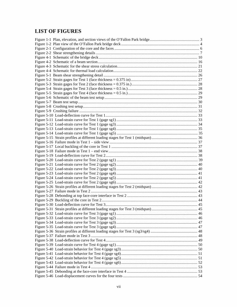
LIST OF FIGURES Figure 1-1 Plan, elevation, and section views of the O’Fallon Park bridge................................................... 3Figure 1-2 Plan view of the O’Fallon Park bridge deck ................................................................................ 4Figure 2-1 Configuration of the core and the faces ....................................................................................... 6Figure 2-2 Shear strengthening details .......................................................................................................... 7Figure 4-1 Schematic of the bridge deck ..................................................................................................... 10Figure 4-2 Schematic of a beam section...................................................................................................... 16Figure 4-3 Schematic for the shear stress calculation.................................................................................. 21Figure 4-4 Schematic for thermal load calculation...................................................................................... 22Figure 5-1 Beam shear strengthening detail ................................................................................................ 26Figure 5-2 Strain gages for Test 1 (face thickness = 0.375 in) .................................................................... 27Figure 5-3 Strain gages for Test 2 (face thickness = 0.375 in.) ................................................................... 28Figure 5-4 Strain gages for Test 3 (face thickness = 0.5 in.) ....................................................................... 28Figure 5-5 Strain gages for Test 4 (face thickness = 0.5 in.) ....................................................................... 29Figure 5-6 Schematic of the beam test setup ............................................................................................... 29Figure 5-7 Beam test setup .......................................................................................................................... 30Figure 5-8 Crushing test setup..................................................................................................................... 31Figure 5-9 Crushing failure ......................................................................................................................... 32Figure 5-10 Load-deflection curve for Test 1.............................................................................................. 33Figure 5-11 Load-strain curve for Test 1 (gage sg1) ................................................................................... 33Figure 5-12 Load-strain curve for Test 1 (gage sg3) ................................................................................... 34Figure 5-13 Load-strain curve for Test 1 (gage sg4) ................................................................................... 35Figure 5-14 Load-strain curve for Test 1 (gage sg5) ................................................................................... 35Figure 5-15 Strain profiles at different loading stages for Test 1 (midspan) ............................................... 36Figure 5-16 Failure mode in Test 1 – side view .......................................................................................... 37Figure 5-17 Local buckling of the core in Test 1 ........................................................................................ 37Figure 5-18 Failure mode in Test 1 – end view........................................................................................... 38Figure 5-19 Load-deflection curve for Test 2.............................................................................................. 38Figure 5-20 Load-strain curve for Test 2 (gage sg1) ................................................................................... 39Figure 5-21 Load-strain curve for Test 2 (gage sg2) ................................................................................... 40Figure 5-22 Load-strain curve for Test 2 (gage sg3) ................................................................................... 40Figure 5-23 Load-strain curve for Test 2 (gage sg4) ................................................................................... 41Figure 5-24 Load-strain curve for Test 2 (gage sg5) ................................................................................... 41Figure 5-25 Load-strain curve for Test 2 (gage sg6) ................................................................................... 42Figure 5-26 Strain profiles at different loading stages for Test 2 (midspan) ............................................... 42Figure 5-27 Failure mode in Test 2 ............................................................................................................. 43Figure 5-28 Debonding at top face-core interface in Test 2 ........................................................................ 43Figure 5-29 Buckling of the core in Test 2.................................................................................................. 44Figure 5-30 Load-deflection curve for Test 3.............................................................................................. 45Figure 5-31 Strain profiles at different loading stages for Test 3 (midspan) ............................................... 45Figure 5-32 Load-strain curve for Test 3 (gage sg1) ................................................................................... 46Figure 5-33 Load-strain curve for Test 3 (gage sg2) ................................................................................... 46Figure 5-34 Load-strain curve for Test 3 (gage sg3) ................................................................................... 47Figure 5-35 Load-strain curve for Test 3 (gage sg4) ................................................................................... 47Figure 5-36 Strain profiles at different loading stages for Test 3 (sg3/sg4) ................................................ 48Figure 5-37 Failure mode in Test 3 ............................................................................................................. 48Figure 5-38 Load-deflection curve for Test 4.............................................................................................. 49Figure 5-39 Load-strain curve for Test 4 (gage sg1) ................................................................................... 50Figure 5-40 Load-strain behavior for Test 4 (gage sg3) .............................................................................. 50Figure 5-41 Load-strain behavior for Test 4 (gage sg4) .............................................................................. 51Figure 5-42 Load-strain behavior for Test 4 (gage sg5) .............................................................................. 51Figure 5-43 Load-strain behavior for Test 4 (gage sg6) .............................................................................. 52Figure 5-44 Failure mode in Test 4 ............................................................................................................. 53Figure 5-45 Debonding at the face-core interface in Test 4 ........................................................................ 53Figure 5-46 Load-displacement curves for the four tests ............................................................................ 54
vii

Figure 6-1 Schematic of the beam analysis ................................................................................................. 57Figure 6-2 Finite element model of the test beams...................................................................................... 59Figure 6-3 Comparison of load-displacement curves from analytical and FE models with experimental
results for Test 1 ................................................................................................................................... 60Figure 6-4 Comparison of load-displacement curves from analytical and FE models with experimental
results for Test 2 ................................................................................................................................... 61Figure 6-5 Comparison of load-displacement curves from analytical and FE models with experimental
results for Test 3 ................................................................................................................................... 61Figure 6-6 Comparison of load-displacement curves from analytical and FE models with experimental
results for Test 4 ................................................................................................................................... 62Figure 6-7 Analytical and numerical load-strain curves for bottom strain at midspan for Test 1 ............... 63Figure 6-8 Analytical and numerical load-strain curves for bottom strain at midspan for Test 2 ............... 63Figure 6-9 Analytical and numerical load-strain curves for bottom strain at midspan for Test 3 ............... 64Figure 6-10 Analytical and numerical load-strain curves for bottom strain at midspan for Test 4 ............. 64Figure 6-11 Analytical and numerical load-strain curves for bottom strain at 7.5 in. from midspan for Test
1 ............................................................................................................................................................ 65Figure 6-12 Analytical and numerical load-strain curves for bottom strain at 7.5 in. from midspan for Test
2 ............................................................................................................................................................ 66Figure 6-13 Analytical and numerical load-strain curves for bottom strain at 7.5 in. from midspan for Test
3 ............................................................................................................................................................ 66Figure 6-14 Analytical and numerical load-strain curves for bottom strain at 7.5 in. from midspan for Test
4 ............................................................................................................................................................ 67Figure 6-15 Strain distribution along the top face of the beam in Test 1 .................................................... 68Figure 6-16 Strain distribution along the top face of the beam in Test 2 .................................................... 69Figure 6-17 Strain distribution along the top and bottom faces of the beam in Test 3 at different loading
stages (only the top stain is shown for the FEA) .................................................................................. 70Figure 6-18 Strain distribution along the top face of the beam in Test 4 .................................................... 71Figure 6-19 Stresses along the interface between the top face and the core of the beam in Test 1 from FE
analysis ................................................................................................................................................. 73Figure 6-20 Maximum and minimum principal stresses for Test 1 from FE analysis................................. 73Figure 6-21 Average shear stress................................................................................................................. 75Figure 6-22 Linear softening law ................................................................................................................ 77Figure 6-23 Finite element mesh for nonlinear fracture mechanics analysis............................................... 78Figure 6-24 Finite element analysis results ................................................................................................. 79Figure 6-25 Deformed shape after failure (Amplification factor of 5) ........................................................ 80Figure 7-1 Panel dimensions (in inches) ..................................................................................................... 81Figure 7-2 Test setup ................................................................................................................................... 82Figure 7-3 Reinforcement details for the supports ...................................................................................... 83Figure 7-4 Support structure........................................................................................................................ 84Figure 7-5 Deck installation procedure ....................................................................................................... 85Figure 7-6 Strain gage locations for the panel test (all dimensions in inches) ............................................ 87Figure 7-7 LVDT positions (all dimensions in inches) ............................................................................... 88Figure 7-8 Cyclic load definition................................................................................................................. 89Figure 7-9 Elevation view of the LVDT locations ...................................................................................... 90Figure 7-10 Load-displacement curves for the initial static test .................................................................. 91Figure 7-11 Deformed shape along line C-C (All dimensions in inches, deflections amplified 30 times).. 92Figure 7-12 Load-vs-actual deflection curves for the initial static test........................................................ 93Figure 7-13 Load-strain curves for the initial static test .............................................................................. 94Figure 7-14 Strain ε11 along line B-B at different loading stages ................................................................ 95Figure 7-15 Strain ε11 along section C-C..................................................................................................... 95Figure 7-16 Picture of the panel local bending............................................................................................ 96Figure 7-17 Panel strain profiles ................................................................................................................. 97Figure 7-18 Membrane tension due to the anchor bolts .............................................................................. 97Figure 7-19 Load-strain curves for all the strain gages at 15,000 cycles..................................................... 99Figure 7-20 Comparison of the load-displacement curves at the initial static test (0k) and between 15,000
and 15,200 cycles ............................................................................................................................... 100
viii
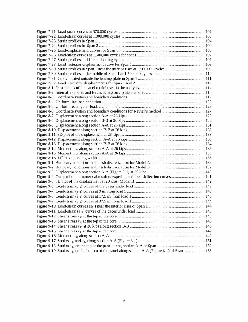
Figure 7-21 Load-strain curves at 370,000 cycles ..................................................................................... 102Figure 7-22 Load-strain curves at 1,000,000 cycles .................................................................................. 103Figure 7-23 Strain profiles in Span 1......................................................................................................... 104Figure 7-24 Strain profiles in Span 2........................................................................................................ 104Figure 7-25 Load-displacement curves for Span 1 .................................................................................... 106Figure 7-26 Load-strain curves at 1,500,000 cycles for span1 .................................................................. 107Figure 7-27 Strain profiles at different loading cycles .............................................................................. 107Figure 7-28 Load- actuator displacement curve for Span 1....................................................................... 108 Figure 7-29 Strain profiles in Span 1 near the interior riser at 1,500,000 cycles....................................... 109Figure 7-30 Strain profiles at the middle of Span 1 at 1,500,000 cycles ................................................... 110Figure 7-31 Crack located outside the loading plate in Span 1 ................................................................. 111Figure 7-32 Load – actuator displacements for Span 1 and 2.................................................................... 112Figure 8-1 Dimensions of the panel model used in the analysis................................................................ 114Figure 8-2 Internal moments and forces acting on a plate element ........................................................... 116Figure 8-3 Coordinate system and boundary conditions ........................................................................... 119 Figure 8-4 Uniform line load condition..................................................................................................... 123Figure 8-5 Uniform rectangular load......................................................................................................... 123Figure 8-6 Coordinate system and boundary conditions for Navier’s method .......................................... 127Figure 8-7 Displacement along section A-A at 26 kips............................................................................. 129Figure 8-8 Displacement along section B-B at 26 kips ............................................................................. 130Figure 8-9 Displacement along section A-A at 26 kips............................................................................. 131Figure 8-10 Displacement along section B-B at 26 kips ........................................................................... 132Figure 8-11 3D plot of the displacement at 26 kips................................................................................... 133Figure 8-12 Displacement along section A-A at 26 kips........................................................................... 133Figure 8-13 Displacement along section B-B at 26 kips ........................................................................... 134Figure 8-14 Moment mx1 along section A-A at 26 kips............................................................................. 135Figure 8-15 Moment mx2 along section A-A at 26 kips............................................................................. 135Figure 8-16 Effective bending width......................................................................................................... 136Figure 9-1 Boundary conditions and mesh discretization for Model A..................................................... 139Figure 9-2 Boundary conditions and mesh discretization for Model B ..................................................... 139Figure 9-3 Displacement along section A-A (Figure 8-1) at 20 kips......................................................... 140Figure 9-4 Comparison of numerical result to experimental load-deflection curves................................. 141Figure 9-5 3D plot of the displacement at 20 kips (Model B) ................................................................... 142Figure 9-6 Load-strain (ε11) curves of the gages under load 1................................................................... 142Figure 9-7 Load-strain (ε11) curves at 9 in. from load 1 ............................................................................ 143Figure 9-8 Load-strain (ε11) curves at 17.5 in. from load 1 ....................................................................... 143Figure 9-9 Load-strain (ε11) curves at 37.5 in. from load 1 ....................................................................... 144Figure 9-10 Load-strain curves (ε11) near the interior riser of Span 1 ....................................................... 144Figure 9-11 Load-strain (ε22) curves of the gages under load 1................................................................. 145Figure 9-12 Shear stress τ13 at the top of the core...................................................................................... 145Figure 9-13 Shear stress τ23 at the top of the core...................................................................................... 146Figure 9-14 Shear stress τ13 at 20 kips along section B-B ......................................................................... 146Figure 9-15 Shear stress τ13 at the top of the core...................................................................................... 147Figure 9-16 Moment mx1 along section A-A ............................................................................................. 149Figure 9-17 Strains ε11 and ε22 along section A-A (Figure 8-1) ................................................................. 151Figure 9-18 Strains ε11 on the top of the panel along section A-A of Span 1 ............................................ 152Figure 9-19 Strains ε11 on the bottom of the panel along section A-A (Figure 8-1) of Span 1.................. 153
ix
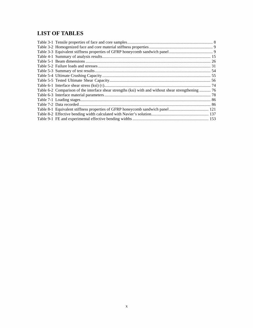
LIST OF TABLES Table 3-1 Tensile properties of face and core samples.................................................................................. 8Table 3-2 Homogenized face and core material stiffness properties ............................................................. 9Table 3-3 Equivalent stiffness properties of GFRP honeycomb sandwich panel .......................................... 9Table 4-1 Summary of analysis results........................................................................................................ 15Table 5-1 Beam dimensions ........................................................................................................................ 26Table 5-2 Failure loads and stresses ............................................................................................................ 31Table 5-3 Summary of test results ............................................................................................................... 54Table 5-4 Ultimate Crushing Capacity ........................................................................................................ 55Table 5-5 Tested Ultimate Shear Capacity................................................................................................. 56Table 6-1 Interface shear stress (ksi) (τ)...................................................................................................... 74Table 6-2 Comparison of the interface shear strengths (ksi) with and without shear strengthening ........... 76Table 6-3 Interface material parameters ...................................................................................................... 78Table 7-1 Loading stages............................................................................................................................. 86Table 7-2 Data recorded .............................................................................................................................. 86Table 8-1 Equivalent stiffness properties of GFRP honeycomb sandwich panel ...................................... 121Table 8-2 Effective bending width calculated with Navier’s solution....................................................... 137Table 9-1 FE and experimental effective bending widths ......................................................................... 153
x

EQUATION CHAPTER 1 SECTION 1
1 INTRODUCTION
1.1 Background
A large number of highway bridges are in need of repair, replacement, or significant
upgrade because of deterioration induced by environmental conditions, increasing traffic
volume, and higher load requirements. In the United States, 50% of all bridges were built
before the 1940’s and approximately 42% of these structures are structurally deficient
(Stallings et al. 2000). Many bridges require upgrades because of a steady increase in the
legal truck weights and traffic volume. Changes in social needs, upgrading of design
standards, and increase in safety requirements lead to the need of major maintenance,
rehabilitation, or reconstruction. In some cases, repair and retrofit will not suffice and
replacement is the only possible solution. In such a case, there are not only the associated
material costs to consider, but also the labor costs, delays, and detours. Hence, a cost-
effective solution must consider the minimization of traffic disruption as well as future
maintenance needs.
Fiber reinforced polymer (FRP) materials offer high stiffness and strength-to-weight
ratios, excellent corrosion and fatigue resistance, reduced maintenance costs, simplicity
of handling, and faster installation time compared to conventional materials. However,
there is still a great need for further research on durability, performance, and testing and
manufacturing standards to develop design guidelines and codes for FRPs, which will
lead to a wider use of the materials and, thereby, reduced costs.
Recently, many state transportation departments in collaboration with the Federal
Highway Administration (FHWA) are working toward the use of FRP materials for
bridge construction. The Innovative Bridge Research and Construction (IBRC) Program
of FHWA was initiated with the aim of promoting the use of innovative materials and
construction technologies in bridges. Under the IRBC program, the City and County of
Denver in cooperation with the Colorado Department of Transportation (CDOT) and
FHWA built a bridge with a glass fiber reinforced polymer deck (GFRP) in O’Fallon
1
Park, which is located west of the City of Denver.
The GFRP deck in the O’Fallon Park bridge is supported on five reinforced concrete
risers built over an arch as shown in Figure 1-1. The total length of the deck is 43.75 ft.
and the width is 16.25 ft. One of the main objectives of this project is to investigate the
feasibility of using FRP decks for highway bridges. Hence, the FRP deck in the O’Fallon
Park bridge was designed to have a configuration similar to a highway bridge deck.
However, the spans between the concrete risers are a bit shorter than those in a typical
highway deck.
The GFRP deck has a sandwich construction with top and bottom faces and a
honeycomb core. The deck comprises six 7.29-ft.-wide and 7.5-in.-thick panels as shown
in Figure 1-1. They were manufactured in a factory, shipped to the site, and assembled by
the supplier, which is Kansas Structural Composites, Inc. (KSCI). The deck is anchored
to the concrete risers with bolts secured by epoxy. There are two anchor bolts on each
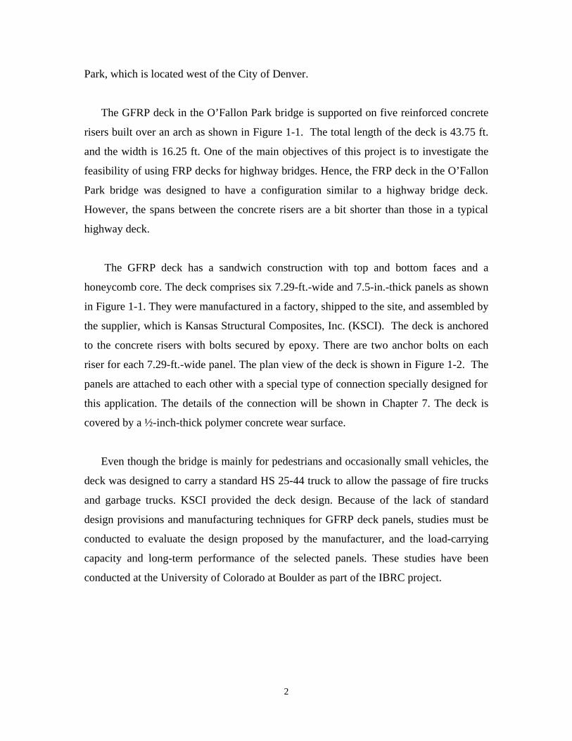
riser for each 7.29-ft.-wide panel. The plan view of the deck is shown in Figure 1-2. The
panels are attached to each other with a special type of connection specially designed for
this application. The details of the connection will be shown in Chapter 7. The deck is
covered by a ½-inch-thick polymer concrete wear surface.
Even though the bridge is mainly for pedestrians and occasionally small vehicles, the
deck was designed to carry a standard HS 25-44 truck to allow the passage of fire trucks
and garbage trucks. KSCI provided the deck design. Because of the lack of standard
design provisions and manufacturing techniques for GFRP deck panels, studies must be
conducted to evaluate the design proposed by the manufacturer, and the load-carrying
capacity and long-term performance of the selected panels. These studies have been
conducted at the University of Colorado at Boulder as part of the IBRC project.
2

Figure 1-1 Plan, elevation, and section views of the O’Fallon Park bridge
3
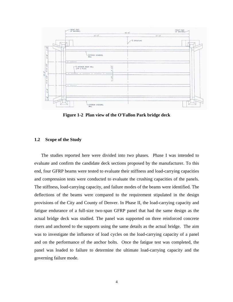
Figure 1-2 Plan view of the O’Fallon Park bridge deck
1.2 Scope of the Study
The studies reported here were divided into two phases. Phase I was intended to
evaluate and confirm the candidate deck sections proposed by the manufacturer. To this
end, four GFRP beams were tested to evaluate their stiffness and load-carrying capacities
and compression tests were conducted to evaluate the crushing capacities of the panels.
The stiffness, load-carrying capacity, and failure modes of the beams were identified. The
deflections of the beams were compared to the requirement stipulated in the design
provisions of the City and County of Denver. In Phase II, the load-carrying capacity and
fatigue endurance of a full-size two-span GFRP panel that had the same design as the
actual bridge deck was studied. The panel was supported on three reinforced concrete
risers and anchored to the supports using the same details as the actual bridge. The aim
was to investigate the influence of load cycles on the load-carrying capacity of a panel
and on the performance of the anchor bolts. Once the fatigue test was completed, the
panel was loaded to failure to determine the ultimate load-carrying capacity and the
governing failure mode.
4

Furthermore, finite element models and analytical models based on the Timoshenko
beam theory and the Kirchhoff-Love plate theory have been developed to obtain a better
understanding of the experimental results and to evaluate the design of the actual deck.
In particular, the load distribution capability of the GFRP deck has been evaluated and
the effective width for shear and bending has been identified.
1.3 Organization of the Report
In Chapter 2, the design, section properties, and manufacturing process of the GFRP
panels used in the O’Fallon Park bridge are briefly summarized. The mechanical
properties of the GFRP materials used in the panels are presented in Chapter 3. In
Chapter 4, the design evaluation conducted on the bridge deck is presented. Chapter 5
presents the experimental studies conducted in Phase I on four simply supported GFRP
beams and the crushing tests performed on four GFRP specimens. In Chapter 6, the
numerical and analytical studies conducted on the test beams with the Timoshenko beam
theory and finite element models are presented. Chapter 7 describes the static load tests
and fatigue test conducted in Phase II on a full-size two-span deck panel that had the
same design as the actual deck. Chapter 8 presents the analytical study conducted on the
test panel with the Kirchhoff-Love plate theory to investigate the load-resisting behavior
of a GFRP deck, including the effective bending width and the influence of material
orthotropy. In Chapter 9, the finite element analyses performed on the test panel are
presented. The analyses are to evaluate the analytical model based on the plate theory, the
influence of the shear deformation of the honeycomb core and support conditions on the
effective bending width, and the design of the actual deck based on the experimental
results. Summary and conclusions are provided in Chapter 10.
5


2 DECK MANUFACTURING PROCESS
This study focuses on the load-carrying behavior of glass fiber reinforced polymer
(GFRP) bridge deck panels manufactured by Kansas Structural Composites, Inc. (KSCI)
using a hand lay-up technique. The deck panels are constructed using a sandwich panel
configuration, which consists of two stiff faces separated by a lightweight core. The
core has a sinusoidal wave configuration in the x1-x2 plane, as shown in Figure 2-1.
h
x1
x2
x3 tc
2 in
.
x1
x2
Core
=0.09 in.
2 in.
Face
(a) Panel (b) RVE
Figure 2-1 Configuration of the core and the faces
The sinusoidal wave has an amplitude of 2 in. and the core material has a thickness
of 0.09 in., as shown in Figure 2-1(b). Figure 2-1(b) shows a Representative Volume
Element (RVE), which is a single basic cell that is repeated periodically to form the core
structure. The panel was designed for one-way bending about the x2 axis. Therefore, the
bending stiffness about the x2 axis is much higher than that about x1.
Plunkett (1997) described in detail the panel manufacturing process. The
honeycomb core is composed of a flat GFRP sheet bonded to a corrugated GFRP sheet as
shown in Figure 2-1. The core flat parts are laid up on a flat surface with vinylester resin
manually applied to chopped strand mat reinforcement. The corrugated parts are
6

fabricated in the same fashion as the flat parts but on corrugated molds. The flat parts are
then placed on top of the wet corrugated parts to produce a bond as the corrugated parts
cure. The face is composed of fiberglass fabric layers, which are wet in resin and laid up
upon each other until desired face thickness is obtained.
To increase the interface shear strength between the core and the faces, a new detail
is introduced in the manufacturing process for the O’Fallon Park bridge panels. In the
panels, GFRP mats are inserted between the core and the faces at about 13 in. distance as
shown in Figure 2-2(b).
CoreCore
Top face
Bottom face
Shear strengthening
13 in.
Top face
Bottom face
Unstrengthened panel
(a) (b)
Figure 2-2 Shear strengthening details
Figure 2-2 shows that the shear strengthening also increases the thickness of the
faces and thereby the bending resistance of the structural members. This must be
considered in analysis.
7
3 MATERIAL PROPERTIES
The honeycomb panels manufactured by Kansas Structural Composites, Inc. (KSCI)
are normally designed for one-way bending about the x2 axis as shown in Figure 2-1. For
this reason, most of the past research has been focused on the tensile properties of the
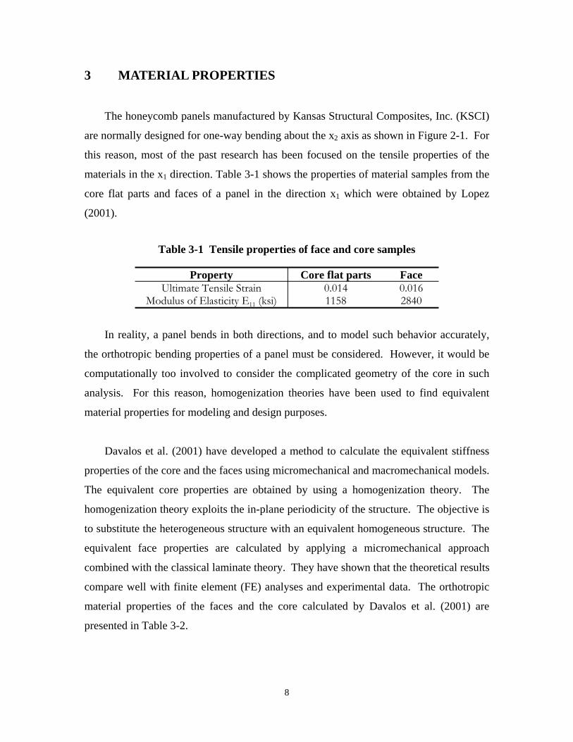
materials in the x1 direction. Table 3-1 shows the properties of material samples from the
core flat parts and faces of a panel in the direction x1 which were obtained by Lopez
(2001).
Table 3-1 Tensile properties of face and core samples
Property Core flat parts Face Ultimate Tensile Strain 0.014 0.016
Modulus of Elasticity E11 (ksi) 1158 2840
In reality, a panel bends in both directions, and to model such behavior accurately,
the orthotropic bending properties of a panel must be considered. However, it would be
computationally too involved to consider the complicated geometry of the core in such
analysis. For this reason, homogenization theories have been used to find equivalent
material properties for modeling and design purposes.
Davalos et al. (2001) have developed a method to calculate the equivalent stiffness
properties of the core and the faces using micromechanical and macromechanical models.
The equivalent core properties are obtained by using a homogenization theory. The
homogenization theory exploits the in-plane periodicity of the structure. The objective is
to substitute the heterogeneous structure with an equivalent homogeneous structure. The
equivalent face properties are calculated by applying a micromechanical approach
combined with the classical laminate theory. They have shown that the theoretical results
compare well with finite element (FE) analyses and experimental data. The orthotropic
material properties of the faces and the core calculated by Davalos et al. (2001) are
presented in Table 3-2.
8
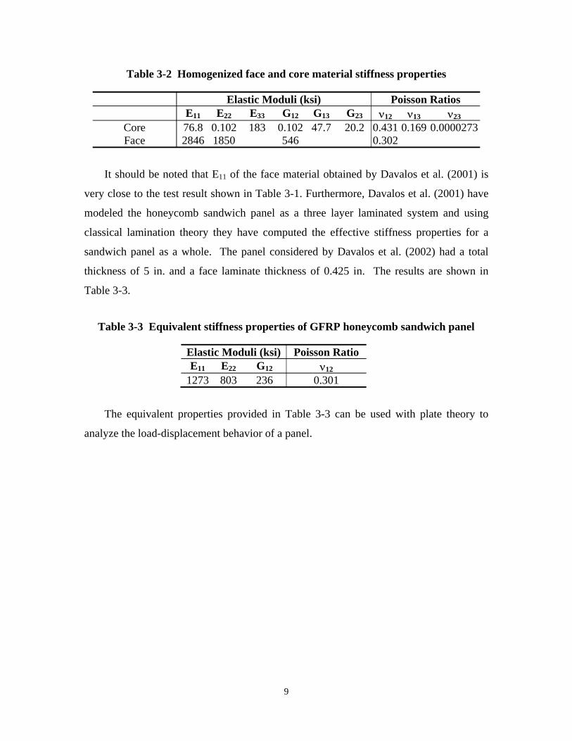
Table 3-2 Homogenized face and core material stiffness properties
Elastic Moduli (ksi) Poisson Ratios E11 E22 E33 G12 G13 G23 ν12 ν13 ν23
Core 76.8 0.102 183 0.102 47.7 20.2 0.431 0.169 0.0000273 Face 2846 1850 546 0.302
It should be noted that E11 of the face material obtained by Davalos et al. (2001) is
very close to the test result shown in Table 3-1. Furthermore, Davalos et al. (2001) have
modeled the honeycomb sandwich panel as a three layer laminated system and using
classical lamination theory they have computed the effective stiffness properties for a
sandwich panel as a whole. The panel considered by Davalos et al. (2002) had a total
thickness of 5 in. and a face laminate thickness of 0.425 in. The results are shown in
Table 3-3.
Table 3-3 Equivalent stiffness properties of GFRP honeycomb sandwich panel
Elastic Moduli (ksi) Poisson Ratio E11 E22 G12 ν12
1273 803 236 0.301
The equivalent properties provided in Table 3-3 can be used with plate theory to
analyze the load-displacement behavior of a panel.
9
EQUATION CHAPTER 4 SECTION 1
PLAN FRP DECK
4 EVALUATION OF DECK DESIGN FOR THE O’FALLON PARK BRIDGE DECK
4.1 General
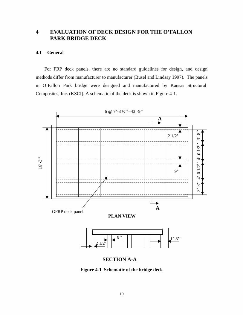
For FRP deck panels, there are no standard guidelines for design, and design
methods differ from manufacturer to manufacturer (Busel and Lindsay 1997). The panels
in O’Fallon Park bridge were designed and manufactured by Kansas Structural
Composites, Inc. (KSCI). A schematic of the deck is shown in Figure 4-1.
A
A
9’’
2 1/2’’
16’-
3’’
6 @ 7’-3 ½’’=43’-9’’
3’-8
’’4’
-0 1
/2’’
4’-0
1/2
’’3’
-8’’
GFRP deck panel PLAN VIEW
9’’ 1’-8’’ 2 1/2’’
SECTION A-A
Figure 4-1 Schematic of the bridge deck
10
Six 16’-3’’ by 7’-3 1/2’’ GFRP panels are used for the bridge deck. The bridge is
owned by the City and County of Denver, which has special design provisions (City and
County of Denver 2002) for the deck. In Section 600 of the provisions, there are
specifications on materials, design requirements, and manufacturing quality control. The
manufacturer designed the deck following these specifications. They initially proposed
several candidate sections for the deck. These sections were evaluated analytically at the
University of Colorado. Two of these sections were later evaluated by beam tests. The
final design was selected based on results of these tests. The following sections describe
the design specifications and the calculations used to examine the different panel sections
proposed by the manufacturer.
4.2 Design Requirements
4.2.1 Structural Loads
For this bridge, the design live load specified is an HS 25 truck. This leads to a
design wheel load of 20 kips. With an impact factor of 30%, the design load becomes 26
kips per wheel.
4.2.2 Tire Contact Area
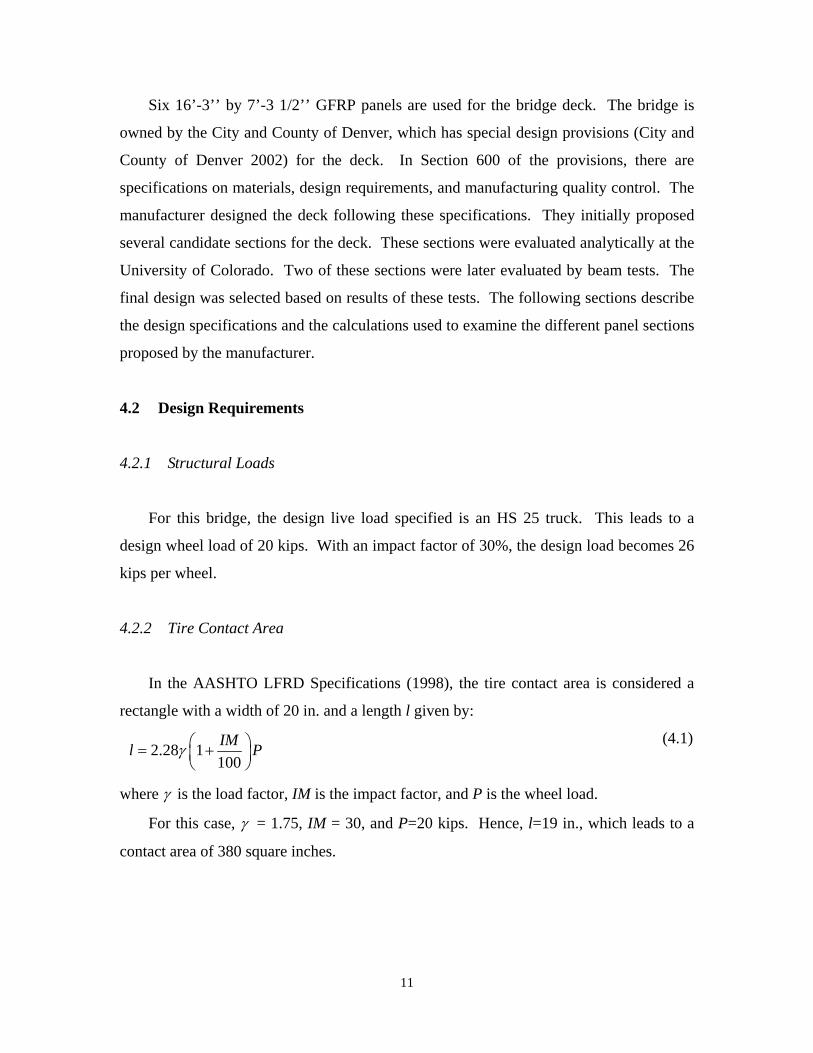
In the AASHTO LFRD Specifications (1998), the tire contact area is considered a
rectangle with a width of 20 in. and a length l given by:
IM (4.1)l = 2.28γ
1 + 100 P
where γ is the load factor, IM is the impact factor, and P is the wheel load.
For this case, γ = 1.75, IM = 30, and P=20 kips. Hence, l=19 in., which leads to a
contact area of 380 square inches.
11
4.2.3 Load Transfer
The load transfer capability of a honeycomb panel is not well understood. Therefore,
to determine the effective width for design, some assumptions are necessary. For this
evaluation, assumptions were made based on the AASHTO Standard Specifications
(1996) for concrete slabs. AASHTO distinguishes between two cases for slabs supported
along two edges: (1) main reinforcement perpendicular to the traffic, and (2) main
reinforcement parallel to the traffic.
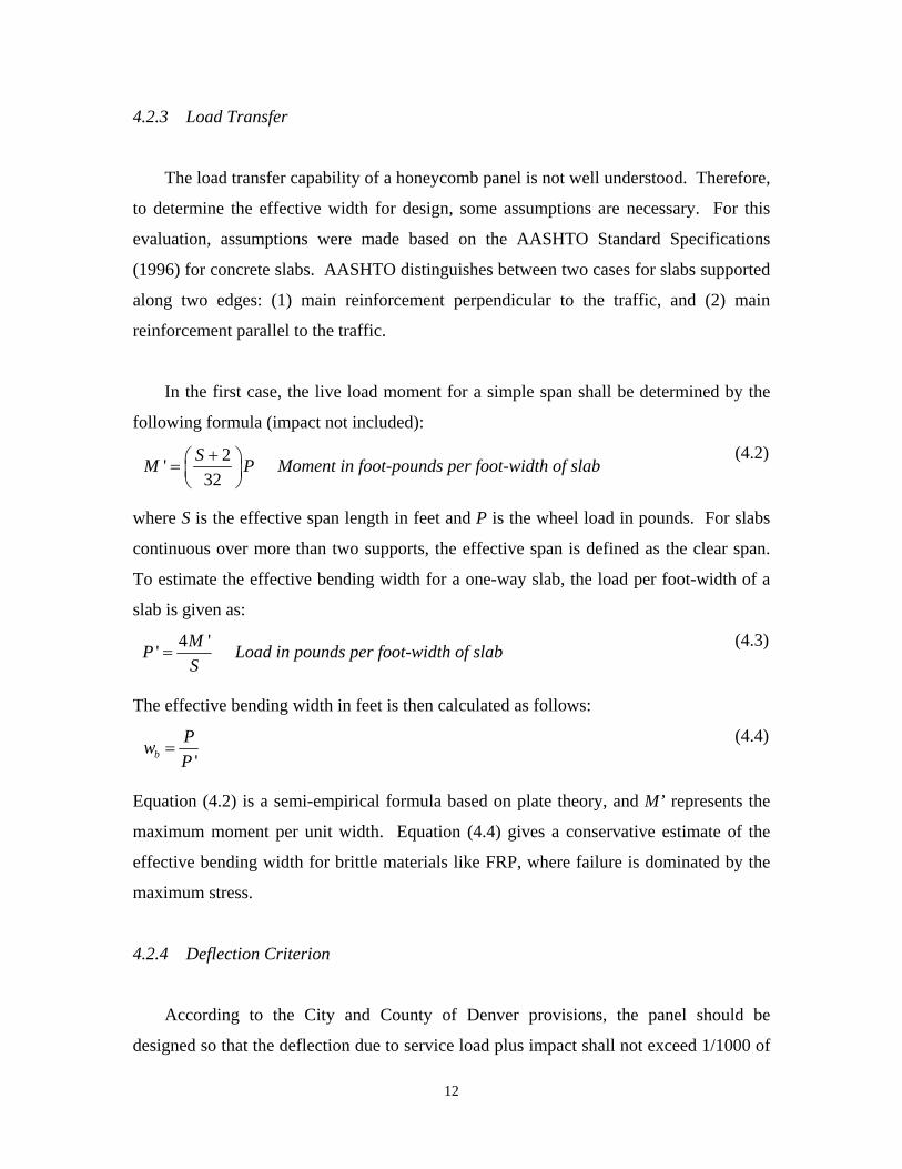
In the first case, the live load moment for a simple span shall be determined by the
following formula (impact not included):
(4.2)M ' =
S + 2 P Moment in foot-pounds per foot-width of slab 32
where S is the effective span length in feet and P is the wheel load in pounds. For slabs
continuous over more than two supports, the effective span is defined as the clear span.
To estimate the effective bending width for a one-way slab, the load per foot-width of a
slab is given as:
4 'MP ' = Load in pounds per foot-width of slab (4.3)
S
The effective bending width in feet is then calculated as follows:
P (4.4)=wb P '
Equation (4.2) is a semi-empirical formula based on plate theory, and M’ represents the
maximum moment per unit width. Equation (4.4) gives a conservative estimate of the
effective bending width for brittle materials like FRP, where failure is dominated by the
maximum stress.
4.2.4 Deflection Criterion
According to the City and County of Denver provisions, the panel should be
designed so that the deflection due to service load plus impact shall not exceed 1/1000 of
12

the span length.
4.2.5 Flexure Criteria
Section 600 of the City and County of Denver provisions suggests using both
Allowable Stress Design and Load Factor Design approaches as follows.
The maximum strain shall be limited to 20% of the ultimate strain under service
loads and the maximum dead load strain shall be limited to 10% of the ultimate strain.
The maximum Factored Load shall be given by:
P = 1.3x(1.67x(LLxIM)+DL)) (4.5)
and it shall not exceed 50% of ultimate load capacity. In equation (4.5), LL is the Live
Load, IM is the Impact Factor, and DL is the Live Load.
In the City and County of Denver provisions, there is no specification on the
effective width of a panel. According to equation (4.4), the effective bending width for
the bridge deck is 5.3 ft. Therefore, in this evaluation, the effective width for bending,
wb, was conservatively assumed to be four feet.
4.2.6 Shear Criteria
The shear failure mode for the honeycomb sandwich panel used for the O’Fallon
bridge deck is expected to be different from that for reinforced concrete (RC) decks.
GFRP sandwich deck fails in shear when a face delaminates from the core, and previous
experimental studies (Stone et al. 2001 and Lopez 2001) have shown that this mode is
most often the governing failure mode for this type of panel.
Section 600 of the City and County of Denver provisions indicates that the maximum
Factored Load shall be given by equation (4.5) and it shall not exceed 45% of the
ultimate shear load capacity of the deck.
13
In this evaluation, the effective width for shear, ws, was assumed to be equal to the
panel width, which is seven feet. This is because delamination in one spot will not
necessarily lead to a complete delamination in a panel. However, results of the study
presented later in this report indicate that this assumption needs to be revisited.
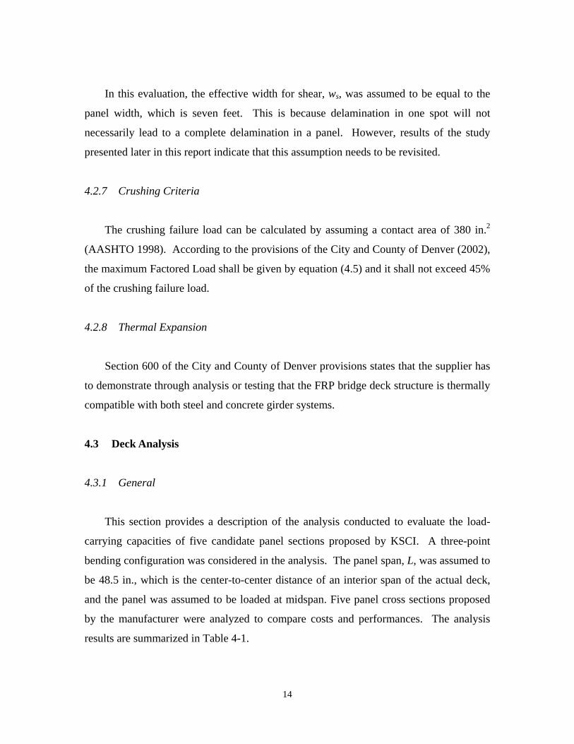
4.2.7 Crushing Criteria
The crushing failure load can be calculated by assuming a contact area of 380 in.2
(AASHTO 1998). According to the provisions of the City and County of Denver (2002),
the maximum Factored Load shall be given by equation (4.5) and it shall not exceed 45%
of the crushing failure load.
4.2.8 Thermal Expansion
Section 600 of the City and County of Denver provisions states that the supplier has
to demonstrate through analysis or testing that the FRP bridge deck structure is thermally
compatible with both steel and concrete girder systems.
4.3 Deck Analysis
4.3.1 General
This section provides a description of the analysis conducted to evaluate the load-
carrying capacities of five candidate panel sections proposed by KSCI. A three-point
bending configuration was considered in the analysis. The panel span, L, was assumed to
be 48.5 in., which is the center-to-center distance of an interior span of the actual deck,
and the panel was assumed to be loaded at midspan. Five panel cross sections proposed
by the manufacturer were analyzed to compare costs and performances. The analysis
results are summarized in Table 4-1.
14
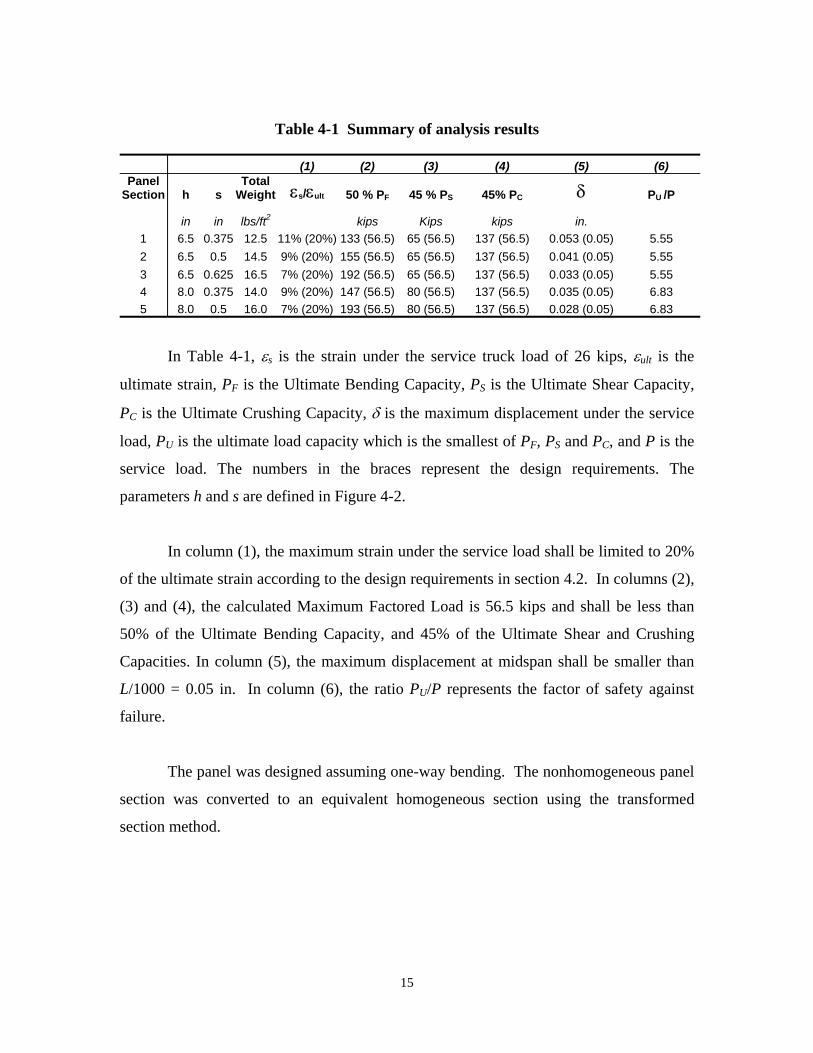
Table 4-1 Summary of analysis results
(1) (2) (3) (4) (5) (6) Panel
Section h s Total
Weight εs/εult 50 % PF 45 % PS 45% PC δ PU /P
in in lbs/ft2 kips Kips kips in. 1 6.5 0.375 12.5 11% (20%) 133 (56.5) 65 (56.5) 137 (56.5) 0.053 (0.05) 5.55 2 6.5 0.5 14.5 9% (20%) 155 (56.5) 65 (56.5) 137 (56.5) 0.041 (0.05) 5.55 3 6.5 0.625 16.5 7% (20%) 192 (56.5) 65 (56.5) 137 (56.5) 0.033 (0.05) 5.55 4 8.0 0.375 14.0 9% (20%) 147 (56.5) 80 (56.5) 137 (56.5) 0.035 (0.05) 6.83 5 8.0 0.5 16.0 7% (20%) 193 (56.5) 80 (56.5) 137 (56.5) 0.028 (0.05) 6.83
In Table 4-1, εs is the strain under the service truck load of 26 kips, εult is the
ultimate strain, PF is the Ultimate Bending Capacity, PS is the Ultimate Shear Capacity,
PC is the Ultimate Crushing Capacity, δ is the maximum displacement under the service
load, PU is the ultimate load capacity which is the smallest of PF, PS and PC, and P is the
service load. The numbers in the braces represent the design requirements. The
parameters h and s are defined in Figure 4-2.
In column (1), the maximum strain under the service load shall be limited to 20%
of the ultimate strain according to the design requirements in section 4.2. In columns (2),
(3) and (4), the calculated Maximum Factored Load is 56.5 kips and shall be less than
50% of the Ultimate Bending Capacity, and 45% of the Ultimate Shear and Crushing
Capacities. In column (5), the maximum displacement at midspan shall be smaller than
L/1000 = 0.05 in. In column (6), the ratio PU/P represents the factor of safety against
failure.
The panel was designed assuming one-way bending. The nonhomogeneous panel
section was converted to an equivalent homogeneous section using the transformed
section method.
15
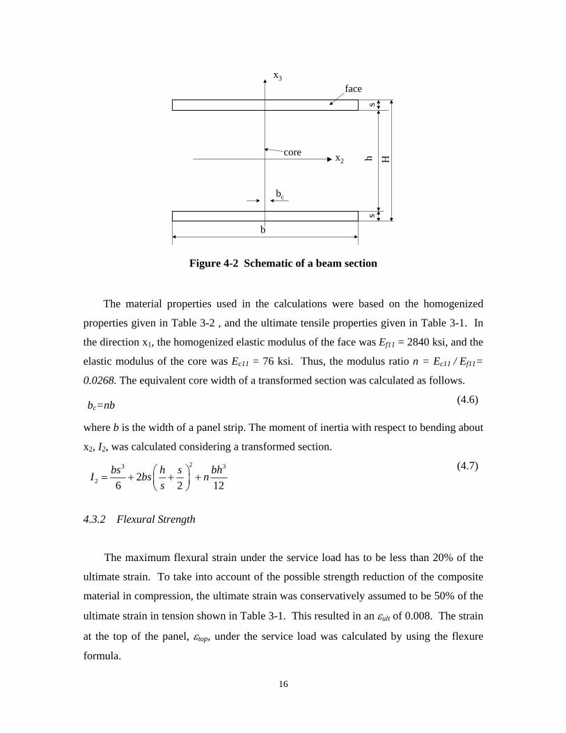
bc
b
h s
s H
face
core x2
x3
Figure 4-2 Schematic of a beam section
The material properties used in the calculations were based on the homogenized
properties given in Table 3-2 , and the ultimate tensile properties given in Table 3-1. In
the direction x1, the homogenized elastic modulus of the face was Ef11 = 2840 ksi, and the
elastic modulus of the core was Ec11 = 76 ksi. Thus, the modulus ratio n = Ec11 / Ef11=
0.0268. The equivalent core width of a transformed section was calculated as follows.
bc=nb (4.6)
where b is the width of a panel strip. The moment of inertia with respect to bending about
x2, I2, was calculated considering a transformed section.
3 3 (4.7)bs h s 2 bhI2 = + 2bs +
2 + n 6 s 12
4.3.2 Flexural Strength
The maximum flexural strain under the service load has to be less than 20% of the
ultimate strain. To take into account of the possible strength reduction of the composite
material in compression, the ultimate strain was conservatively assumed to be 50% of the
ultimate strain in tension shown in Table 3-1. This resulted in an εult of 0.008. The strain
at the top of the panel, εtop, under the service load was calculated by using the flexure
formula.
16
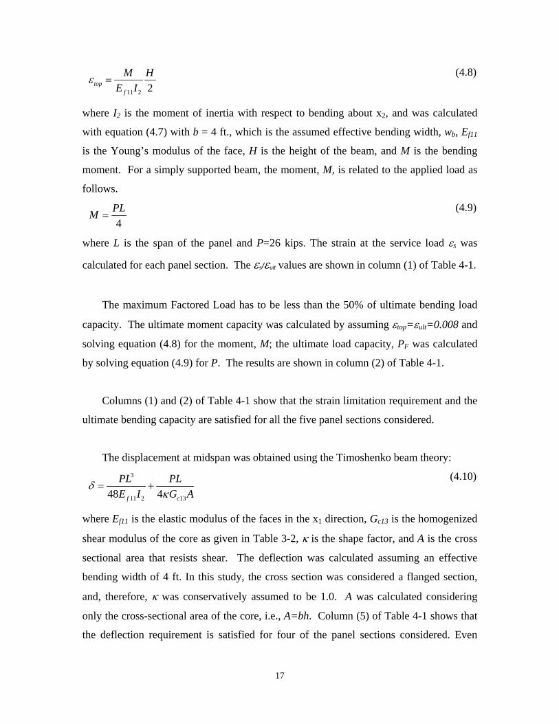
ε = M H (4.8)
top E I2 2f 11
where I2 is the moment of inertia with respect to bending about x2, and was calculated
with equation (4.7) with b = 4 ft., which is the assumed effective bending width, wb, Ef11
is the Young’s modulus of the face, H is the height of the beam, and M is the bending
moment. For a simply supported beam, the moment, M, is related to the applied load as
follows.
PL (4.9)M =
4
where L is the span of the panel and P=26 kips. The strain at the service load εs was
calculated for each panel section. The ε εs/ ult values are shown in column (1) of Table 4-1.
The maximum Factored Load has to be less than the 50% of ultimate bending load
capacity. The ultimate moment capacity was calculated by assuming εtop=εult=0.008 and
solving equation (4.8) for the moment, M; the ultimate load capacity, PF was calculated
by solving equation (4.9) for P. The results are shown in column (2) of Table 4-1.
Columns (1) and (2) of Table 4-1 show that the strain limitation requirement and the
ultimate bending capacity are satisfied for all the five panel sections considered.
The displacement at midspan was obtained using the Timoshenko beam theory:
PL3 PL (4.10)δ = +
48E I2 4κGc13 Af 11
where Ef11 is the elastic modulus of the faces in the x1 direction, Gc13 is the homogenized
shear modulus of the core as given in Table 3-2, κ is the shape factor, and A is the cross
sectional area that resists shear. The deflection was calculated assuming an effective
bending width of 4 ft. In this study, the cross section was considered a flanged section,
and, therefore, κ was conservatively assumed to be 1.0. A was calculated considering
only the cross-sectional area of the core, i.e., A=bh. Column (5) of Table 4-1 shows that
the deflection requirement is satisfied for four of the panel sections considered. Even
17
though the first panel section slightly violates this requirement, it is considered
acceptable as the analysis is based on a conservative assumption of a panel simply
supported along two edges. In the actual bridge, the panel is continuous over five
supports.
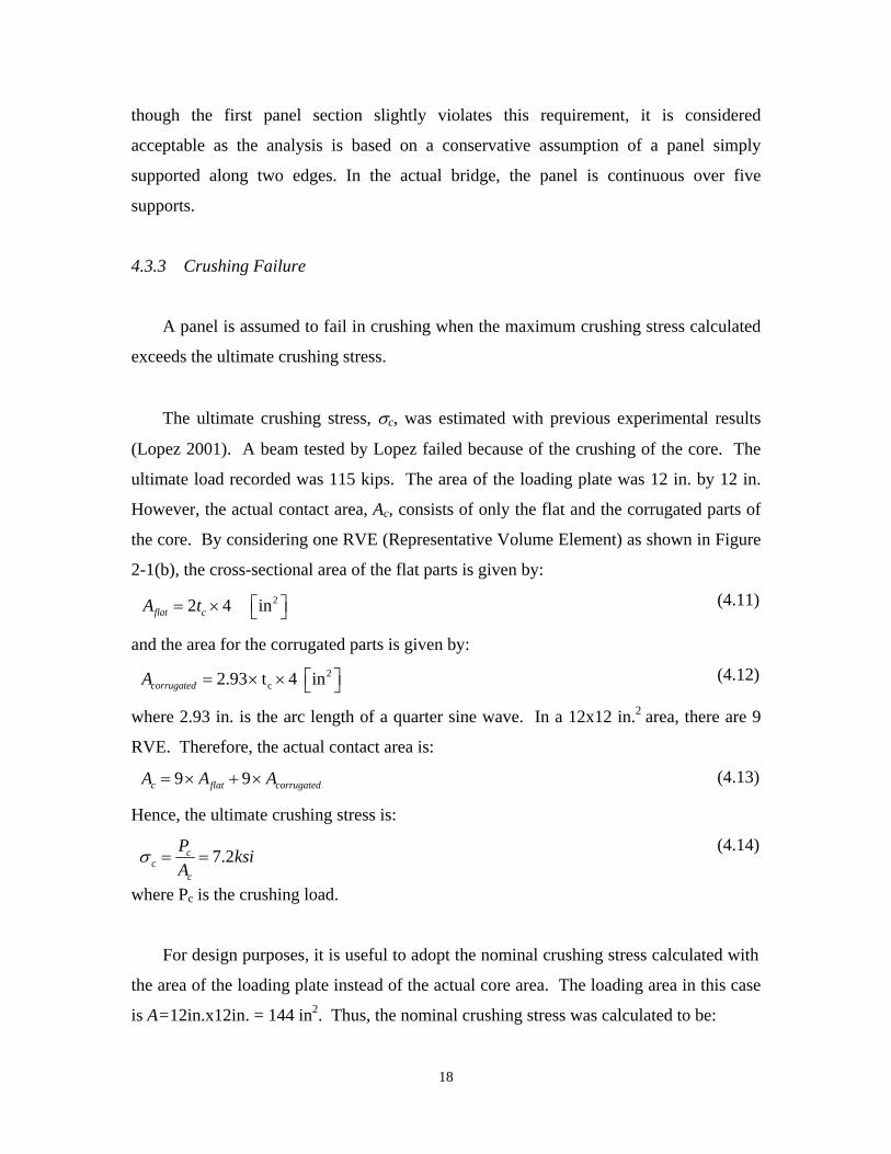
4.3.3 Crushing Failure
A panel is assumed to fail in crushing when the maximum crushing stress calculated
exceeds the ultimate crushing stress.
The ultimate crushing stress, σc, was estimated with previous experimental results
(Lopez 2001). A beam tested by Lopez failed because of the crushing of the core. The
ultimate load recorded was 115 kips. The area of the loading plate was 12 in. by 12 in.
However, the actual contact area, Ac, consists of only the flat and the corrugated parts of
the core. By considering one RVE (Representative Volume Element) as shown in Figure
2-1(b), the cross-sectional area of the flat parts is given by:
in2Aflat = 2t × 4 (4.11)c
and the area for the corrugated parts is given by:
(4.12)t 4 in2Acorrugated = 2.93 × × c
where 2.93 in. is the arc length of a quarter sine wave. In a 12x12 in.2 area, there are 9
RVE. Therefore, the actual contact area is:
9 9 (4.13)Ac = × Aflat + × Acorrugated
Hence, the ultimate crushing stress is:
P (4.14)σ = c = 7.2ksi c Ac
where Pc is the crushing load.
For design purposes, it is useful to adopt the nominal crushing stress calculated with
the area of the loading plate instead of the actual core area. The loading area in this case
is A=12in.x12in. = 144 in2. Thus, the nominal crushing stress was calculated to be:
18
c Pσ = = 0.8 ksi (4.15)
, Ac nom
The beam tested by Lopez (2001) was 2.5-ft. deep and had 0.5-in.-thick top and
bottom faces. Since core crushing is very much governed by the geometric stability, a
deeper core is expected to have a lower crushing load. Hence, the nominal crushing stress
shown in equation (4.16) was deemed conservative for the panels considered here and
was, therefore, adopted. The ultimate crushing capacity for the panels was calculated by
assuming a tire contact area of 380 in.2 (AASHTO 1998). The results are shown in
column (4) of Table 4-1. The maximum Factored Load has to be less than the 45% of the
ultimate load capacity, and column (4) of Table 4-1 indicates that this requirement is
satisfied for the panel sections considered.
4.3.4 Shear Failure
The shear failure of a GFRP sandwich panel is quite different from the shear failure
observed for reinforced concrete structures. Based on the published literature, the failure
of GFRP panels manufactured by KSCI is normally triggered by the delamination of the
top face from the core. In this report, such a failure mode is considered shear failure.
Hence, a GFRP panel is considered to fail in shear when the shear stress at the interface
between the face and the core reaches the interface shear strength.
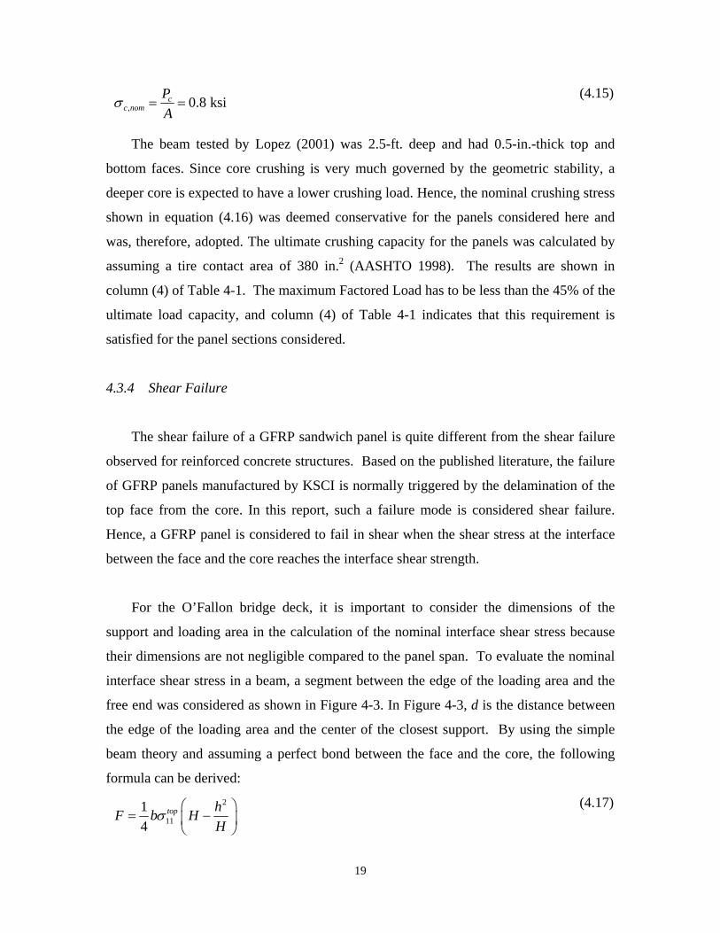
For the O’Fallon bridge deck, it is important to consider the dimensions of the
support and loading area in the calculation of the nominal interface shear stress because
their dimensions are not negligible compared to the panel span. To evaluate the nominal
interface shear stress in a beam, a segment between the edge of the loading area and the
free end was considered as shown in Figure 4-3. In Figure 4-3, d is the distance between
the edge of the loading area and the center of the closest support. By using the simple
beam theory and assuming a perfect bond between the face and the core, the following
formula can be derived:
1 top h2 (4.17)F = bσ 11 H −
H 4
19

where F is the force acting on the face at a distance d due to bending as indicated in
Figure 4-3, σ top is the nominal stress in direction x1 at the top of the face, and b, H and h11
are dimensions defined in Figure 4-3.
σ
The bending stress at the top of the beam is given by:
11 = PH d
(4.18)top
4I2
int To calculate the nominal shear stress, τ , at the interface between the face and the 13
core, the following equation is used:
int F =
F (4.19)τ 13 =
A xb s
where b is the nominal width and x is the distance between the end of the panel and the
edge of the loading area as indicated in Figure 4-3. By substituting equation (4.18) in int (4.17), and then substituting equation (4.17) in (4.19), the nominal shear stress, τ can be13
expressed as:
h2 (4.20)int =
PdH H −
H τ 13 16I2 x
The shear stress calculated with equation (4.20) is considered as the nominal
shear stress. The nominal width, b, was chosen because the actual contact width was
difficult to determine with the new shear strengthening detail shown in Figure 2-2.
20

P/2
d
F tτ ττττ
x
b
Core
Face
A
A
Section A-A
hH
τ τ
Figure 4-3 Schematic for the shear stress calculation
The Ultimate Shear Capacity, PS, is defined as the load at which the nominal
interface shear stress is equal to the ultimate shear strength, τ ult. Thus, by rearranging int equation (4.20) and letting τ =τ ult, we have:13
16I x = 2PS d H 2 − h2 )
τ ult (4.21)
(
For the O’Fallon Park deck, the b value used to calculate I2 was assumed to be 7 ft.,
which was the assumed effective width for shear, the tire contact width perpendicular to
the direction of the traffic is 20 in. (AASHTO 1998), and the support for the deck is 9 in.
wide. Hence, with the conservative assumption that the deck has a simply supported span
of 48.5 in. and that the wheel load is at midspan, x is 18.75 in. and d is 14.25 in.
The ultimate interface shear strength, τ ult, was estimated from the results of the four
beam tests conducted by Lopez (2001) and Stone et al. (2001). By using equation (4.20),
the nominal shear stress at failure was calculated to be 0.08 and 0.085 ksi for the two
beams tested by Lopez, and 0.14 and 0.21 ksi for the beams tested by Stone et al.
Because of the small number of data available, the lowest shear stress of 0.08 ksi was
used as the ultimate shear strength for the analysis here.
The maximum Factored Load has to be less than the 45% of the Ultimate Shear
21

Capacity, and Column (3) of Table 4-1 indicates that this requirement is satisfied for all
the panel sections considered.
Moreover, it must be mentioned that the manufacturer of the O’Fallon Park bridge
deck had improved the interface shear strength by providing a shear strengthening detail
as shown in Figure 2-2. The beam tests presented later in this report show that the new
shear strengthening method can indeed substantially increase the face-core interface shear
strength.
4.3.5 Thermal Effect
For FRP structures, the thermal effect could be a critical factor. For the continuous
panels in the O’Fallon Park bridge, thermal stresses introduced by the differential
temperature across a panel section could be significant. For this reason, a thermal
analysis was conducted by assuming a severe temperature differential of ∆T = = 50 ºF,
between the top and bottom faces of a panel. Figure 4-4 shows a two-span continuum
deck considered in this analysis. The thermal stresses can be calculated with the
principle of superposition by first removing the center support and reapplying the support
reaction P as shown in Figure 4-4.
L
x θ
0
L
L L
δ
P
y,w
therm
Figure 4-4 Schematic for thermal load calculation
22

The coefficient of thermal expansion given by the manufacturer is α = 28x10-6 /
ºC. The curvature induced by a thermal gradient is given by the following equation:
φ =α∆ T (4.22)
H The rotation of an infinitesimal segment is thus obtained as:
dθ =α∆ T (4.23)
dx H
and the deflection at midspan can be found by applying the principle of Virtual Work:
therm L L 1 α∆ Tδ = 2∫ 0 M dθ = 2 x dx
(4.24) v ∫ 0 2 H
where Mv is the virtual moment due to a unit point load applied at midspan in the same
direction as the displacement δ.
Therefore, the deflection at midspan is:
δ therm =α∆ TL2 (4.25)
2H
The deflection due to the force P applied at midspan as shown in Figure 4-4 is:
8PL3 (4.26)δ =
48E I2f 11
δ therm By having = δ , the force P is found as follows:
P = 3α∆TE f 11I2 (4.27)
HL
The shear stress due to the force P obtained with equation (4.27) can be calculated int with equation (4.20). For a differential temperature of 50 ºF, the shear stress, τ , is 0.0113
ksi for panel section 1, 0.01 ksi for panel section 2, 0.02 ksi for panel section 3, 0.01 ksi
for panel section 4, and 0.02 ksi for panel section 5. These are lower than the assumed
ultimate shear strength of 0.08 ksi.
23

4.4 Summary
In summary, all five panel sections considered here satisfy the design requirements
of Section 4.2. Panel sections 1 and 2 were chosen for further evaluation with beam tests
because they provide the required structural performance, light weight, and desired panel
depths.
24

EQUATION CHAPTER 6 SECTION 1
5 BEAM TESTS
5.1 Introduction
Section 600 of the City and County of Denver provisions requires performance
testing of samples of deck panels selected for the O’Fallon Park bridge. To this end,
beam specimens were tested at the University of Colorado at Boulder to evaluate the
stiffness and ultimate load capacity of different panel sections.
The tests followed the procedures specified in Section 600 of the City and County of
Denver provisions. The beams were tested under third-point loading with a span of 48.5
in., which is the span length of the actual bridge deck. However, the actual deck spans
continuously over five reinforced concrete risers as shown in Figure 1-1.
Section 600 of the City and County of Denver provisions requires that the midspan
deflection of a one-foot-wide beam shall not exceed 1/500 of the clear span when
subjected to a point load of 10,000 lbs. In addition, the provisions require that the
sections shall be loaded until failure to evaluate the ultimate load capacity of the
specimens. The following sections describe the test specimens, test setup, and results.
5.2 Test Specimens
A total of four beams, which represented candidate sections for the deck panels of
the O’Fallon Park bridge, were tested in bending using third-point loading. Based on the
evaluation presented in Chapter 4, two types of beam sections were selected with two for
each type. All the beams had a core height of 6.5 in. Two of the beams had 0.375-in.
faces and the remaining two 0.5-in. faces as shown in Table 5-1. The section with 0.375-
in. faces is the lightest section that satisfies the design requirements. The beams were
wrapped with external layers of GFRP to increase the shear resistance at the core-face
interface as shown in Figure 5-1.
25
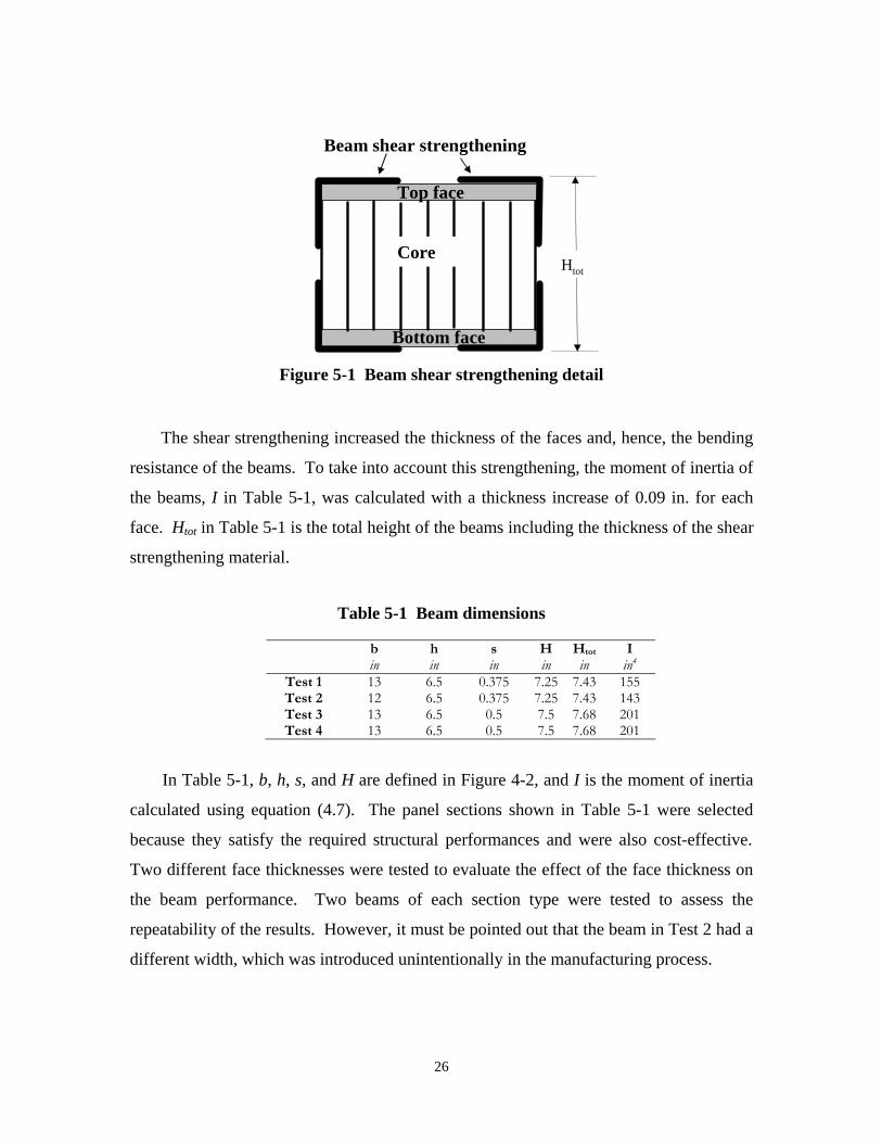
Core H
Top face
Bottom face
Beam shear strengthening
tot
Figure 5-1 Beam shear strengthening detail
The shear strengthening increased the thickness of the faces and, hence, the bending
resistance of the beams. To take into account this strengthening, the moment of inertia of
the beams, I in Table 5-1, was calculated with a thickness increase of 0.09 in. for each
face. Htot in Table 5-1 is the total height of the beams including the thickness of the shear
strengthening material.
Table 5-1 Beam dimensions
b h s H Htot I in in in in in in4
Test 1 13 6.5 0.375 7.25 7.43 155 Test 2 12 6.5 0.375 7.25 7.43 143 Test 3 13 6.5 0.5 7.5 7.68 201 Test 4 13 6.5 0.5 7.5 7.68 201
In Table 5-1, b, h, s, and H are defined in Figure 4-2, and I is the moment of inertia
calculated using equation (4.7). The panel sections shown in Table 5-1 were selected
because they satisfy the required structural performances and were also cost-effective.
Two different face thicknesses were tested to evaluate the effect of the face thickness on
the beam performance. Two beams of each section type were tested to assess the
repeatability of the results. However, it must be pointed out that the beam in Test 2 had a
different width, which was introduced unintentionally in the manufacturing process.
26

5.3 Instrumentation
Electrical high precision strain gages produced by Micro Measurements Group, Inc.,
with a resistance of 350 ohms, were used along with M-Bond Type AE 10 adhesive
system to measure strains in the axial direction of the beams. Deflection at midspan was
monitored using a Linear Variable Differential Transformer (LVDT). Mechanical dial-
gauges were mounted to check the LVDT readings. Displacement, strain and load
readings were recorded during the tests using a data acquisition system. Figures 5-2 to
Figure 5-5 show a schematic of the strain gauge locations for the four beam tests. Test 1
and Test 3 had gages glued on the front and back of the beams, whereas Test 2 and Test 4
had gages only on the front. The gages on the top and bottom faces were located right at
the center of the face.
0.68 in
3.74 in
7.30 in
7.20 in
1.06 in
Elevation View
Back
Test 1
sg1
sg3
sg2
sg4
sg5
sg6
Front CLCL
Figure 5-2 Strain gages for Test 1 (face thickness = 0.375 in)
27
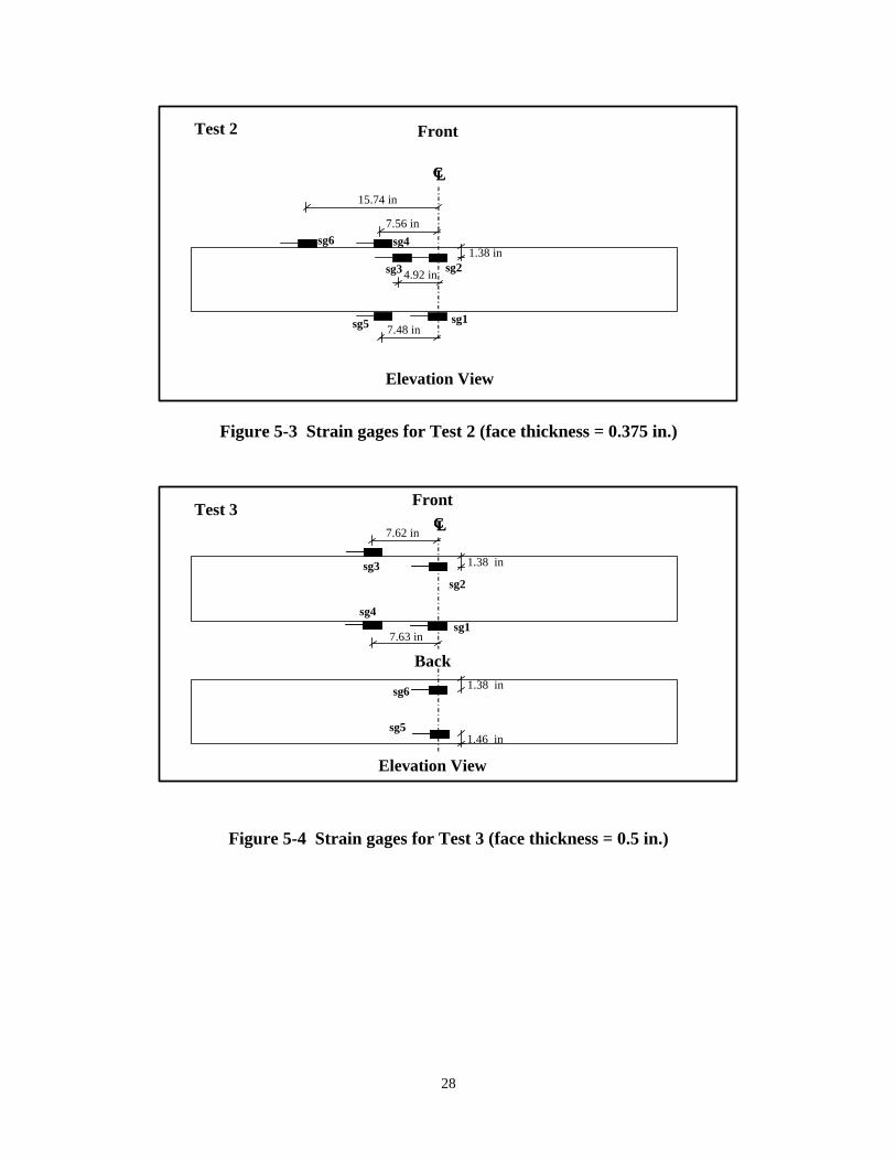
Test 2
1.38 in
7.56 in
4.92 in
15.74 in
7.48 in sg1
sg2sg3
sg4
sg5
sg6
Elevation View
Front
CLCL
Figure 5-3 Strain gages for Test 2 (face thickness = 0.375 in.)
1.38 in
7.62 in
7.63 in
1.38 in
Front
Back
Test 3
1.46 in
sg1
sg2 sg3
sg4
sg5
sg6
Elevation View
CLCL
Figure 5-4 Strain gages for Test 3 (face thickness = 0.5 in.)
28
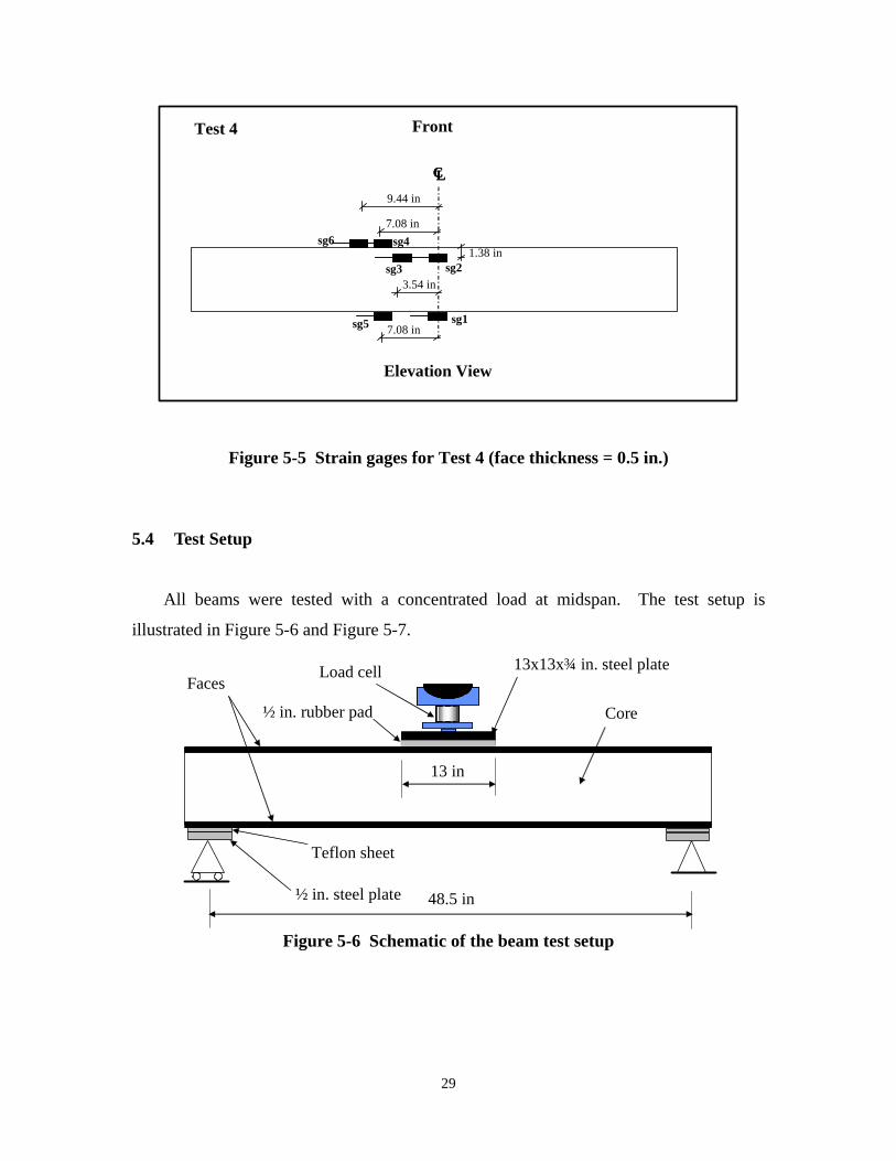
FrontTest 4
1.38 in
7.08 in
3.54 in
9.44 in
7.08 in sg1
sg2sg3
sg4
sg5
sg6
Elevation View
CLCL
Figure 5-5 Strain gages for Test 4 (face thickness = 0.5 in.)
5.4 Test Setup
All beams were tested with a concentrated load at midspan. The test setup is
illustrated in Figure 5-6 and Figure 5-7.
13x13x¾ in. steel plateLoad cellFaces
Core
48.5 in
13 in
½ in. rubber pad
Teflon sheet
½ in. steel plate
Figure 5-6 Schematic of the beam test setup
29

Figure 5-7 Beam test setup
The beams were simply supported on rollers at each end and the load was distributed
uniformly using a 13x13x3/4-in. steel plate. The beams were tested using a rate of
loading of approximately 0.0075 in./min. Data was recorded at a rate of one sample per
second using a 16-channel data-acquisition system.
Crushing tests were also conducted on small panel samples to evaluate the uniaxial
compression strength. The following sections present the results of the crushing tests and
bending tests.
5.5 Crushing Tests
The manufacturer provided four 13-in.-by-12-in. specimens for crushing tests. Like
the beam specimens, the height of the core was 6.5 in. Two were manufactured with
0.375-in. face and two with 0.5-in. face. They were fabricated together with the beams
and were cut from the originally longer beams specimens. An MTS machine with a load
capacity of one million pounds was used. All the specimens were tested under
displacement control. The aim of these tests was to find the ultimate crushing load of the
specimens.
30
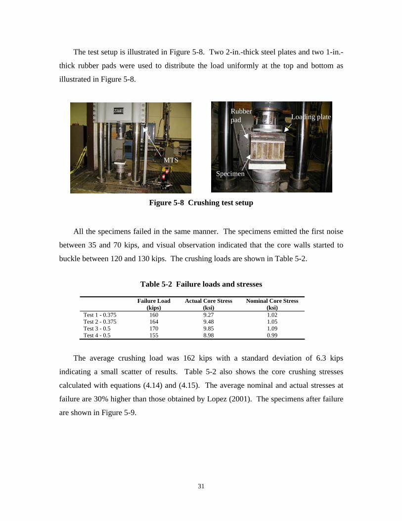
The test setup is illustrated in Figure 5-8. Two 2-in.-thick steel plates and two 1-in.-
thick rubber pads were used to distribute the load uniformly at the top and bottom as
illustrated in Figure 5-8.
MTS
Loading plate
Specimen
Rubber pad
Figure 5-8 Crushing test setup
All the specimens failed in the same manner. The specimens emitted the first noise
between 35 and 70 kips, and visual observation indicated that the core walls started to
buckle between 120 and 130 kips. The crushing loads are shown in Table 5-2.
Table 5-2 Failure loads and stresses
Failure Load Actual Core Stress Nominal Core Stress (kips) (ksi) (ksi)
Test 1 - 0.375 160 9.27 1.02 Test 2 - 0.375 164 9.48 1.05 Test 3 - 0.5 170 9.85 1.09 Test 4 - 0.5 155 8.98 0.99
The average crushing load was 162 kips with a standard deviation of 6.3 kips
indicating a small scatter of results. Table 5-2 also shows the core crushing stresses
calculated with equations (4.14) and (4.15). The average nominal and actual stresses at
failure are 30% higher than those obtained by Lopez (2001). The specimens after failure
are shown in Figure 5-9.
31
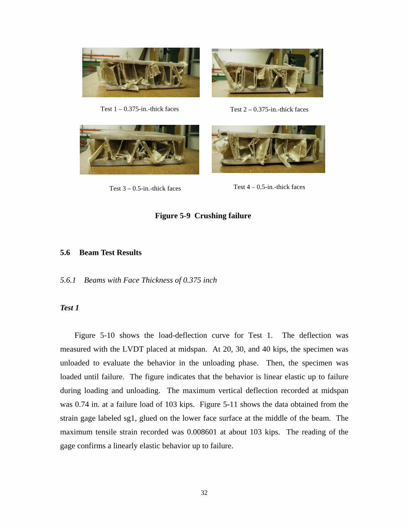
Test 3- 0.500 in. face thickness
Test 2- 0.375 in. face thickness
Test 4- 0.500 in. face thickness
Test 1- 0.375 in. face thicknessTest 1 – 0.375-in.-thick faces Test 2 – 0.375-in.-thick faces
Test 3 – 0.5-in.-thick faces Test 4 – 0.5-in.-thick faces
Figure 5-9 Crushing failure
5.6 Beam Test Results
5.6.1 Beams with Face Thickness of 0.375 inch
Test 1
Figure 5-10 shows the load-deflection curve for Test 1. The deflection was
measured with the LVDT placed at midspan. At 20, 30, and 40 kips, the specimen was
unloaded to evaluate the behavior in the unloading phase. Then, the specimen was
loaded until failure. The figure indicates that the behavior is linear elastic up to failure
during loading and unloading. The maximum vertical deflection recorded at midspan
was 0.74 in. at a failure load of 103 kips. Figure 5-11 shows the data obtained from the
strain gage labeled sg1, glued on the lower face surface at the middle of the beam. The
maximum tensile strain recorded was 0.008601 at about 103 kips. The reading of the
gage confirms a linearly elastic behavior up to failure.
32

0.375 - test1140
70 Lo
ad (k
ips)
Lo
ad (k
ips)
0
)Test 1 (0.375 in. face
0.00 0.20 0.40 0.60 0.80 1.00 Mid-Span Deflection (in)
Figure 5-10 Load-deflection curve for Test 1
140
70
0 0.000 0.003 0.005 0.008 0.010
Strain
) sg1 Test 1 (0.375 in. face
Figure 5-11 Load-strain curve for Test 1 (gage sg1)
Figure 5-12 shows the data obtained from the strain gage labeled sg3, glued on the
side near the top face at the middle of the beam. In this case, the maximum compressive
strain recorded at 103 kips was -0.007426. Considering that the gage was glued at 0.68
in. from the top surface, the calculated maximum compressive strain on the upper surface
was -0.00912 using the plane-section assumption. This value agrees well with the
maximum tensile strain recorded at the bottom face.
33
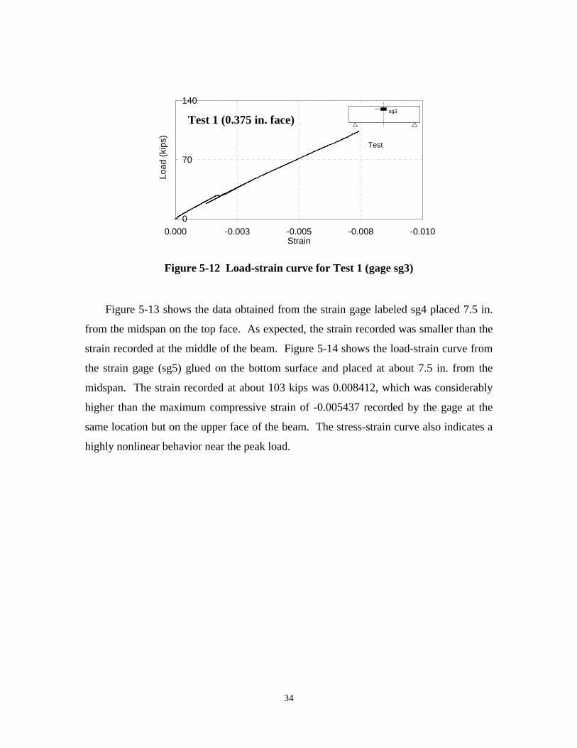
0.375 - test1
0
70
140
)Lo
ad (k
ips Test
sg3
Test 1 (0.375 in. face)
0.000 -0.003 -0.005 -0.008 -0.010 Strain
Figure 5-12 Load-strain curve for Test 1 (gage sg3)
Figure 5-13 shows the data obtained from the strain gage labeled sg4 placed 7.5 in.
from the midspan on the top face. As expected, the strain recorded was smaller than the
strain recorded at the middle of the beam. Figure 5-14 shows the load-strain curve from
the strain gage (sg5) glued on the bottom surface and placed at about 7.5 in. from the
midspan. The strain recorded at about 103 kips was 0.008412, which was considerably
higher than the maximum compressive strain of -0.005437 recorded by the gage at the
same location but on the upper face of the beam. The stress-strain curve also indicates a
highly nonlinear behavior near the peak load.
34

0.375 - test1
0.375 - test1
0
70
140
Load
(kip
s)
) sg4
Test 1 (0.375 in. face
0.000 -0.003 -0.005 -0.008 -0.010 Strain
Figure 5-13 Load-strain curve for Test 1 (gage sg4)
0
70
Load
(kip
s)
) 140
sg5 Test 1 (0.375 in. face
0.000 0.003 0.005 0.008 0.010 Strain
Figure 5-14 Load-strain curve for Test 1 (gage sg5)
The strain profiles at midspan shown in Figure 5-15 indicate that plane sections
remained plane during bending. Figure 5-15 shows that the neutral axis shifted down
right after reaching the 103-kip load indicating the delamination of the top face from the
core.
35

-3.750
3.750
-2.250
-0.750
0.750
2.250
-0.010-0.0050.0000.010
ii-3.715
0.005
Bea
m D
epth
, H (i
n)
20 kips 60 k105 k103 kips
Failure
Test 1 (0.375 in. face)
Middle of the cross section
3.715
ps ps Strain
Figure 5-15 Strain profiles at different loading stages for Test 1 (midspan)
During the test, several types of damage occurred. At about 25 kips, a first noise was
heard indicating that some fibers were breaking. In fact, the load-strain curve from strain
gage sg3 exhibits some nonlinearity at about 27 kips as shown in Figure 5-12.
Throughout the rest of the test, noises were heard indicating that fibers were probably
breaking continuously during loading. Inspection of the beam after failure showed the
presence of loose fibers. Finally, at a load of 103 kips, the top face started delaminating.
The failure was brittle and released a large amount of energy. Debonding between the
core and the upper face started under the load and propagated outward along the top core-
face interface as shown in Figure 5-16. After that, the top face debonded. The core was
subsequently subjected to a larger load which caused the local buckling of the core at
both sides of the beam as illustrated in Figure 5-17. After failure, the top face and the
core were completely detached as shown in Figure 5-18.
36
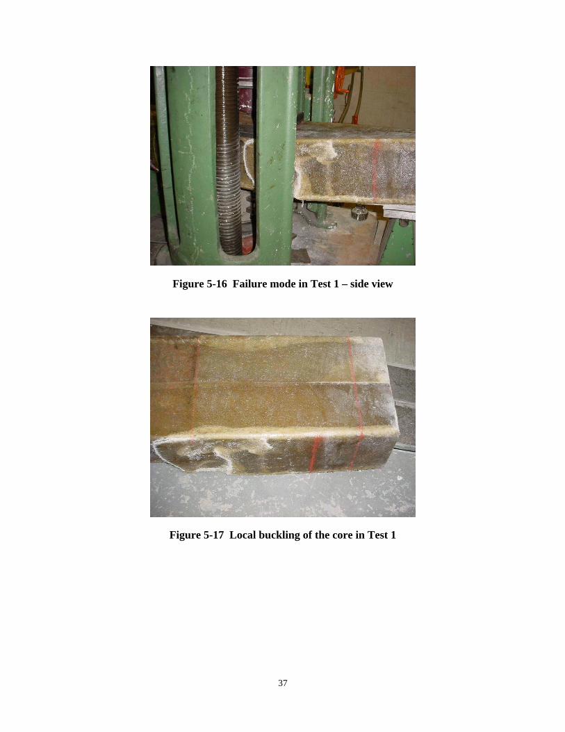
Figure 5-16 Failure mode in Test 1 – side view
Figure 5-17 Local buckling of the core in Test 1
37
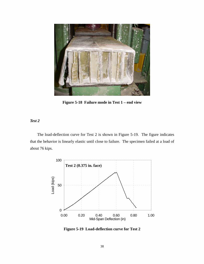
0.375 - test2
Test
Load
(kip
s)
Figure 5-18 Failure mode in Test 1 – end view
Test 2
The load-deflection curve for Test 2 is shown in Figure 5-19. The figure indicates
that the behavior is linearly elastic until close to failure. The specimen failed at a load of
about 76 kips.
100
50
0
)Test 2 (0.375 in. face
0.00 0.20 0.40 0.60 0.80 1.00 Mid-Span Deflection (in)
Figure 5-19 Load-deflection curve for Test 2
38

0.375 - test2
Figure 5-20 shows the data recorded by the strain gage labeled sg1, which was glued
on the bottom face surface at the middle of the beam. The maximum tensile strain
recorded was 0.006438 at about 76 kips. Lo
ad (k
ips)
100
50
0 0.0000 0.0020 0.0040 0.0060 0.0080
Strain
sg1
)
Test
Test 2 (0.375 in. face
Figure 5-20 Load-strain curve for Test 2 (gage sg1)
Figure 5-21 shows the data obtained from the strain gage labeled sg2, glued on the
side near the top face at the middle of the beam. The load-strain curve is not linear. The
maximum compressive strain recorded at 76 kips was -0.004231, and the maximum
compressive strain on the upper surface calculated from this value based on the plane
section assumption is -0.006694, which is very similar to the maximum tensile strain
recorded.
39
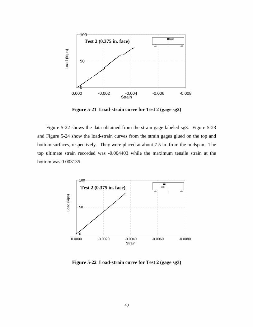
0.375 - test2
0.375 - test2
0
50
100
Load
(kip
s)
sg2)Test 2 (0.375 in. face
0.000 -0.002 -0.004 -0.006 -0.008 Strain
Figure 5-21 Load-strain curve for Test 2 (gage sg2)
Figure 5-22 shows the data obtained from the strain gage labeled sg3. Figure 5-23
and Figure 5-24 show the load-strain curves from the strain gages glued on the top and
bottom surfaces, respectively. They were placed at about 7.5 in. from the midspan. The
top ultimate strain recorded was -0.004403 while the maximum tensile strain at the
bottom was 0.003135.
0
50
100
Load
(kip
s)
) sg3 Test 2 (0.375 in. face
0.0000 -0.0020 -0.0040 -0.0060 -0.0080 Strain
Figure 5-22 Load-strain curve for Test 2 (gage sg3)
40
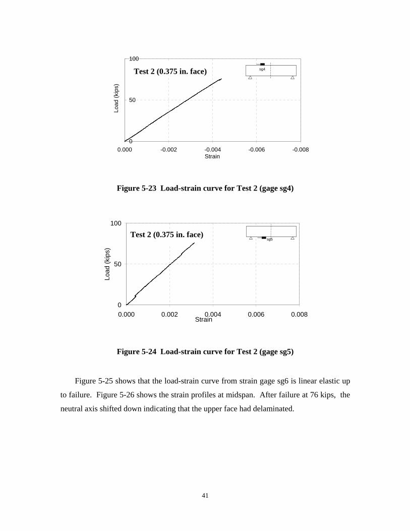
0.375 - test2
0.375 - test2
0
50
100
)
sg4)
Load
(kip
s
Test 2 (0.375 in. face
0.000 -0.002 -0.004 -0.006 -0.008 Strain
Figure 5-23 Load-strain curve for Test 2 (gage sg4)
0
50
Load
(kip
s)
) 100
sg5 Test 2 (0.375 in. face
0.000 0.002 0.004 0.006 0.008Strain
Figure 5-24 Load-strain curve for Test 2 (gage sg5)
Figure 5-25 shows that the load-strain curve from strain gage sg6 is linear elastic up
to failure. Figure 5-26 shows the strain profiles at midspan. After failure at 76 kips, the
neutral axis shifted down indicating that the upper face had delaminated.
41
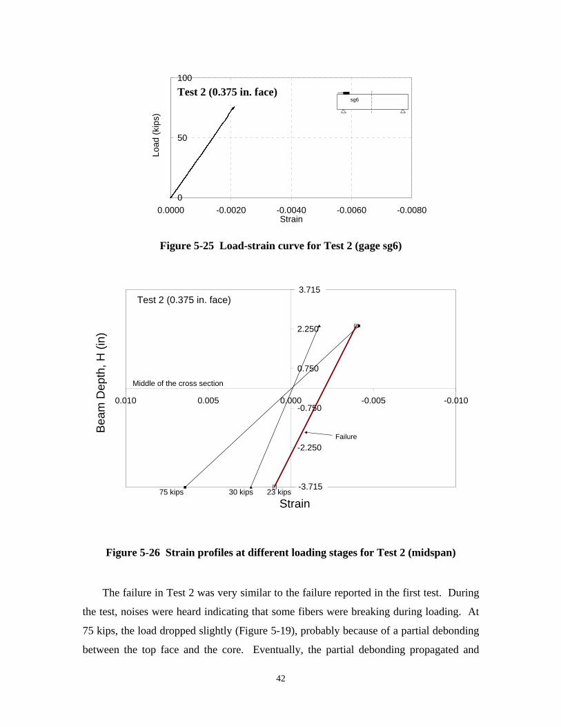
0.375 - test2
Test
-3.750
3.750
0
50
100
Load
(kip
s)
) sg6
Test 2 (0.375 in. face
0.0000 -0.0020 -0.0040 -0.0060 -0.0080 Strain
Figure 5-25 Load-strain curve for Test 2 (gage sg6)
-2.250
-0.750 -0.010
in 75 kips 30 kips
-3.715
0.750
2.250
-0.005 0.000 0.005 0.010
Stra
Bea
m D
epth
, H (i
n)
23 kips
Failure
Middle of the cross section
Test 2 (0.375 in. face) 3.715
Figure 5-26 Strain profiles at different loading stages for Test 2 (midspan)
The failure in Test 2 was very similar to the failure reported in the first test. During
the test, noises were heard indicating that some fibers were breaking during loading. At
75 kips, the load dropped slightly (Figure 5-19), probably because of a partial debonding
between the top face and the core. Eventually, the partial debonding propagated and
42
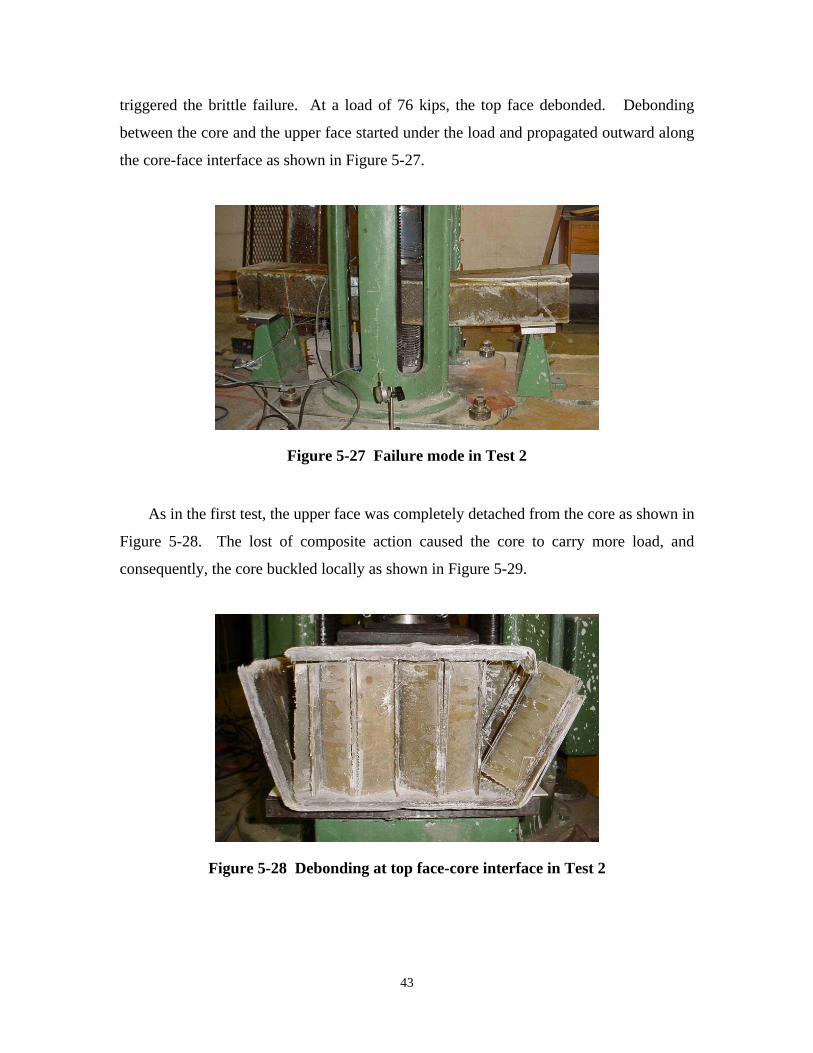
triggered the brittle failure. At a load of 76 kips, the top face debonded. Debonding
between the core and the upper face started under the load and propagated outward along
the core-face interface as shown in Figure 5-27.
Figure 5-27 Failure mode in Test 2
As in the first test, the upper face was completely detached from the core as shown in
Figure 5-28. The lost of composite action caused the core to carry more load, and
consequently, the core buckled locally as shown in Figure 5-29.
Figure 5-28 Debonding at top face-core interface in Test 2
43
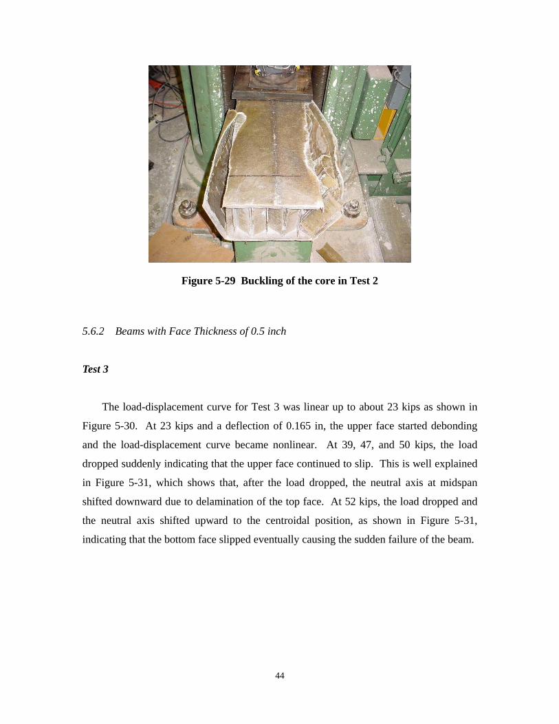
Figure 5-29 Buckling of the core in Test 2
5.6.2 Beams with Face Thickness of 0.5 inch
Test 3
The load-displacement curve for Test 3 was linear up to about 23 kips as shown in
Figure 5-30. At 23 kips and a deflection of 0.165 in, the upper face started debonding
and the load-displacement curve became nonlinear. At 39, 47, and 50 kips, the load
dropped suddenly indicating that the upper face continued to slip. This is well explained
in Figure 5-31, which shows that, after the load dropped, the neutral axis at midspan
shifted downward due to delamination of the top face. At 52 kips, the load dropped and
the neutral axis shifted upward to the centroidal position, as shown in Figure 5-31,
indicating that the bottom face slipped eventually causing the sudden failure of the beam.
44
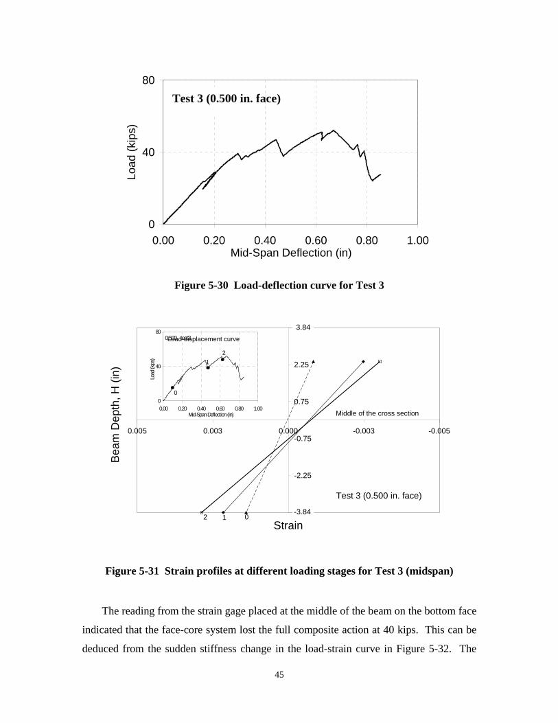
0.500 - test3
-3.75
3.75
0
40
80
Load
(kip
s)
)Test 3 (0.500 in. face
0.00 0.20 0.40 0.60 0.80 1.00 Mid-Span Deflection (in)
Figure 5-30 Load-deflection curve for Test 3
Bea
m D
epth
, H (i
n)
0
40
80
Mi l ion (in)
(kips
)
012
)
1
0
2
-3.84
3.84
-2.25
-0.75
0.75
2.25
-0.005 -0.003 0.000 0.003 0.005
0.00 0.20 0.40 0.60 0.80 1.00 d-Span Defect
Load
0.500 test3 Load-displacement curve
Test 3 (0.500 in. face
Middle of the cross section
Strain
Figure 5-31 Strain profiles at different loading stages for Test 3 (midspan)
The reading from the strain gage placed at the middle of the beam on the bottom face
indicated that the face-core system lost the full composite action at 40 kips. This can be
deduced from the sudden stiffness change in the load-strain curve in Figure 5-32. The
45
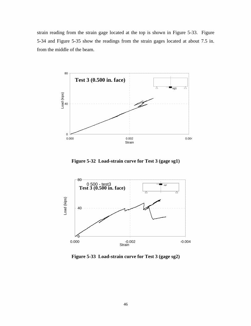
.
strain reading from the strain gage located at the top is shown in Figure 5-33. Figure
5-34 and Figure 5-35 show the readings from the strain gages located at about 7.5 in.
from the middle of the beam.
80
40
Load
(kip
s)
sg1
Test 3 (0.500 in. face)
0 0.000 0.002 0.004
Strain
Figure 5-32 Load-strain curve for Test 3 (gage sg1)
0
40
80
Load
(kip
s)
0 500 - test3 sg2
Test 3 (0.500 in. face)
0.000 -0.002 -0.004 Strain
Figure 5-33 Load-strain curve for Test 3 (gage sg2)
46

0.500 - test3
0.500 - test3
0
40
80
Load
(kip
s)
) sg3
Test 3 (0.500 in. face
0.000 -0.002 -0.004 Strain
Figure 5-34 Load-strain curve for Test 3 (gage sg3)
80
40
Load
(kip
s)
sg4 Test 3 (0.500 in. face)
0 0.000 0.002 0.004
Strain
Figure 5-35 Load-strain curve for Test 3 (gage sg4)
Up to about 39 kips, the load-strain curves for gages sg3 and sg4 show a constant
stiffness, as for the gages sg1 and sg2. At the section were these gages were located, the
neutral axis did not change position up to the peak load as shown in Figure 5-36. This
indicates that, in the beginning, the slip was localized at the middle and, later, it
propagated toward the end of the beam.
47

-3.75
3.75
-0.0050.0000.003
Bea
m D
epth
, H (i
n)
0
40
80
Mi l ion (in)
i)
1 2
2 1 -3.84
-2.25
-0.75
0.75
2.25
-0.003 0.005
0.00 0.20 0.40 0.60 0.80 1.00 d-Span Def ect
Load
(kps
Load-displacement curve
Test 3 (0.500 in. face)
Middle of the cross section
3.84
Strain
Figure 5-36 Strain profiles at different loading stages for Test 3 (sg3/sg4)
The failure observed in Test 3 was different from the failures reported in the
previous tests. The beam failure was pseudo-ductile. The face debonded from the core
progressively starting at 36 kips. The delamination started at the top of midspan and
propagated toward the end of the beam. The top face did not debond uniformly and only
the back side of the core buckled as shown in Figure 5-37.
Figure 5-37 Failure mode in Test 3
48

0.500 - test4
This failure mechanism is probably due to workmanship in the manufacturing
process. The bond between the top face and the core was not of uniform quality and this
induced the premature debonding. This decreased the strength of the beam as compared
to the two previous beams. After the test, visual inspection of the beam showed that one
side of the face was completely debonded from the core. Lo
ad (k
ips)
Test 4
The load-displacement curve for Test 4 is perfectly linear up to 108 kips as shown in
Figure 5-38. From 108 kips up to failure, the load-displacement curve becomes slightly
nonlinear. The beam failed at 131 kips with a deflection of 0.76 in.
140
70
0
)Test 4 (0.500 in. face
0.00 0.20 0.40 0.60 0.80 1.00 Mid-Span Deflection (in)
Figure 5-38 Load-deflection curve for Test 4
The strain gage located at midspan under the beam indicated that the response was
linear elastic up to 108 kips as shown in Figure 5-39. The gage probably failed at a
smaller load level than the beam. This may be due to gage malfunctioning or a localized
failure (some fibers might have broken at this location).
49
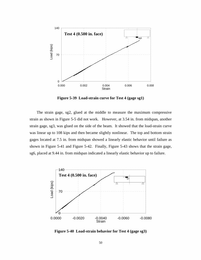
0.500 - test4
0
70Lo
ad (k
ips)
sg1 )
140
Test 4 (0.500 in. face
0.000 0.002 0.004 0.006 0.008 Strain
Figure 5-39 Load-strain curve for Test 4 (gage sg1)
The strain gage, sg2, glued at the middle to measure the maximum compressive
strain as shown in Figure 5-5 did not work. However, at 3.54 in. from midspan, another
strain gage, sg3, was glued on the side of the beam. It showed that the load-strain curve
was linear up to 108 kips and then became slightly nonlinear. The top and bottom strain
gages located at 7.5 in. from midspan showed a linearly elastic behavior until failure as
shown in Figure 5-41 and Figure 5-42. Finally, Figure 5-43 shows that the strain gage,
sg6, placed at 9.44 in. from midspan indicated a linearly elastic behavior up to failure.
0
70
140
Load
(kip
s) sg3
Test 4 (0.500 in. face)
0.0000 -0.0020 -0.0040 -0.0060 -0.0080 Strain
Figure 5-40 Load-strain behavior for Test 4 (gage sg3)
50

0.500 - test4
0.500 - test4
0
70
sg4140
Load
(kip
s)
Test 4 (0.500 in. face)
0.000 -0.002 -0.004 -0.006 -0.008 Strain
Figure 5-41 Load-strain behavior for Test 4 (gage sg4)
0
70
140
Load
(kip
s)
)
sg5
Test 4 (0.500 in. face
0.000 0.002 0.004 0.006 0.008 Strain
Figure 5-42 Load-strain behavior for Test 4 (gage sg5)
51
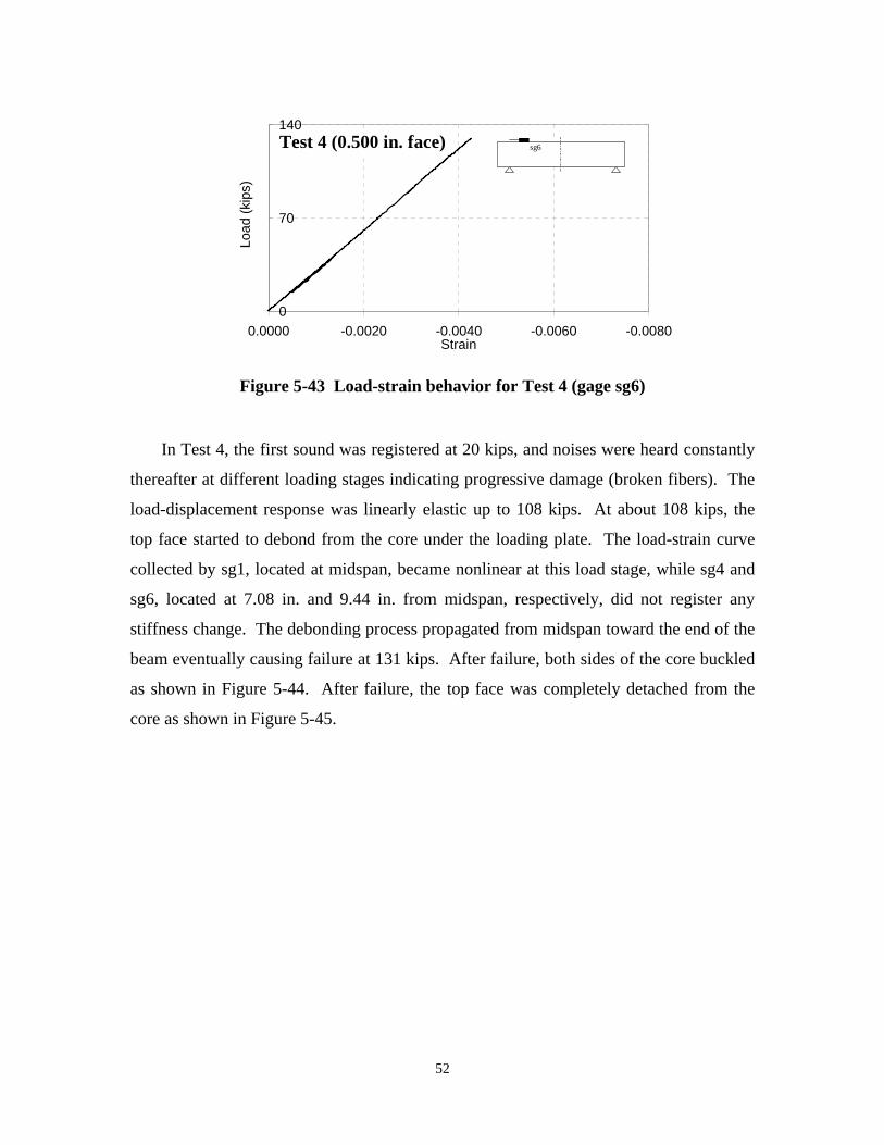
0.500 - test4
0
70
Load
(kip
s)
) 140
sg6 Test 4 (0.500 in. face
0.0000 -0.0020 -0.0040 -0.0060 -0.0080 Strain
Figure 5-43 Load-strain behavior for Test 4 (gage sg6)
In Test 4, the first sound was registered at 20 kips, and noises were heard constantly
thereafter at different loading stages indicating progressive damage (broken fibers). The
load-displacement response was linearly elastic up to 108 kips. At about 108 kips, the
top face started to debond from the core under the loading plate. The load-strain curve
collected by sg1, located at midspan, became nonlinear at this load stage, while sg4 and
sg6, located at 7.08 in. and 9.44 in. from midspan, respectively, did not register any
stiffness change. The debonding process propagated from midspan toward the end of the
beam eventually causing failure at 131 kips. After failure, both sides of the core buckled
as shown in Figure 5-44. After failure, the top face was completely detached from the
core as shown in Figure 5-45.
52
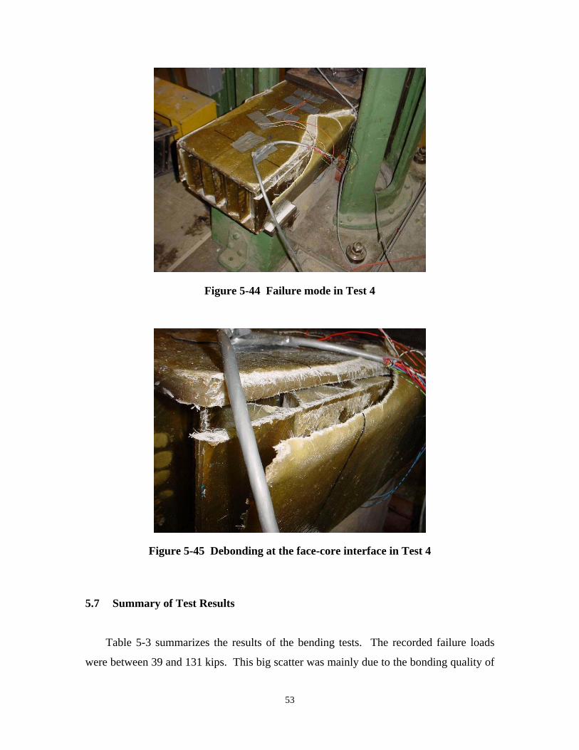
Figure 5-44 Failure mode in Test 4
Figure 5-45 Debonding at the face-core interface in Test 4
5.7 Summary of Test Results
Table 5-3 summarizes the results of the bending tests. The recorded failure loads
were between 39 and 131 kips. This big scatter was mainly due to the bonding quality of
53

the face-core interface.
Table 5-3 Summary of test results
Test Moment of Failure Max displ. L/δ Failure Max top strain at Inertia load (δ) Mode midspan
in4 kips in x1000 1 - 0.375 in. 155 103 0.71 69 1 -8.1822 2 - 0.375 in. 143 76 0.60 80 1 -6.0838 3 - 0.5 in. 201 39 0.29 167 2 -2.4924 4 - 0.5 in. 201 131 0.76 64 1 -7.0055
Load
(kip
s)
In Table 5-3, the maximum top strain in Test 4 was recorded 3.54 in. from midspan
(gage sg3), L is the beam span, and δ is the maximum displacement. The maximum
strain at the top of the beam is calculated with the gage readings taken along the depth of
the beams based on the plane-section assumption. Failure mode 1 represents a linearly
elastic behavior till failure, and failure mode 2 represents a pseudo-ductile behavior with
progressive damage.
Figure 5-46 shows the load-displacement curves for the four tests. The figure shows
that the face thickness influenced the stiffness of the beams as reflected by their moment
of inertia shown in Table 5-3.
150
100
50
0
Test 4
Test1
Test2
Test 3
0.00 0.20 0.40 0.60 0.80 1.00 Mid-Span Deflection (in)
Figure 5-46 Load-displacement curves for the four tests
54
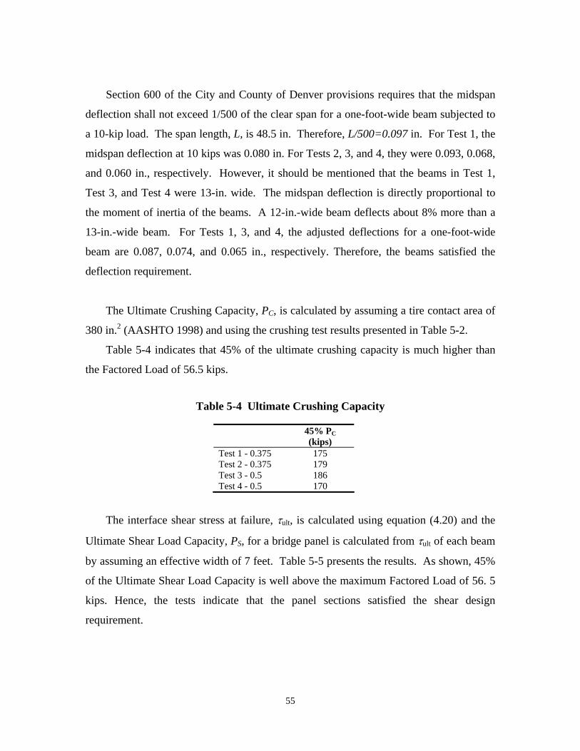
Section 600 of the City and County of Denver provisions requires that the midspan
deflection shall not exceed 1/500 of the clear span for a one-foot-wide beam subjected to
a 10-kip load. The span length, L, is 48.5 in. Therefore, L/500=0.097 in. For Test 1, the
midspan deflection at 10 kips was 0.080 in. For Tests 2, 3, and 4, they were 0.093, 0.068,
and 0.060 in., respectively. However, it should be mentioned that the beams in Test 1,
Test 3, and Test 4 were 13-in. wide. The midspan deflection is directly proportional to
the moment of inertia of the beams. A 12-in.-wide beam deflects about 8% more than a
13-in.-wide beam. For Tests 1, 3, and 4, the adjusted deflections for a one-foot-wide
beam are 0.087, 0.074, and 0.065 in., respectively. Therefore, the beams satisfied the
deflection requirement.
The Ultimate Crushing Capacity, PC, is calculated by assuming a tire contact area of
380 in.2 (AASHTO 1998) and using the crushing test results presented in Table 5-2.
Table 5-4 indicates that 45% of the ultimate crushing capacity is much higher than
the Factored Load of 56.5 kips.
Table 5-4 Ultimate Crushing Capacity
45% PC (kips)
Test 1 - 0.375 175 Test 2 - 0.375 179 Test 3 - 0.5 186 Test 4 - 0.5 170
The interface shear stress at failure, τult, is calculated using equation (4.20) and the
Ultimate Shear Load Capacity, PS, for a bridge panel is calculated from τult of each beam
by assuming an effective width of 7 feet. Table 5-5 presents the results. As shown, 45%
of the Ultimate Shear Load Capacity is well above the maximum Factored Load of 56. 5
kips. Hence, the tests indicate that the panel sections satisfied the shear design
requirement.
55
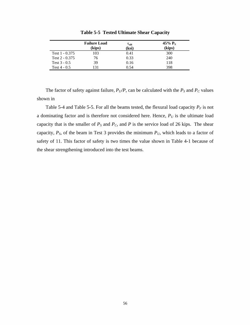
Table 5-5 Tested Ultimate Shear Capacity
Failure Load τult 45% PS (kips) (ksi) (kips)
Test 1 - 0.375 103 0.41 300 Test 2 - 0.375 76 0.33 240 Test 3 - 0.5 39 0.16 118 Test 4 - 0.5 131 0.54 398
The factor of safety against failure, PU/P, can be calculated with the PS and PC values
shown in
Table 5-4 and Table 5-5. For all the beams tested, the flexural load capacity PF is not
a dominating factor and is therefore not considered here. Hence, PU is the ultimate load
capacity that is the smaller of PS and PC, and P is the service load of 26 kips. The shear
capacity, PS, of the beam in Test 3 provides the minimum PU, which leads to a factor of
safety of 11. This factor of safety is two times the value shown in Table 4-1 because of
the shear strengthening introduced into the test beams.
56

6 BEAM ANALYSES
6.1 Introduction
The Timoshenko beam theory and the finite element method are used to analyze the
behavior of the beams that were tested. The following sections give a description of the
analysis models used and the comparison of the theoretical results with experimental
data.
6.2 Timoshenko Beam Theory
Because of the low span-to-depth ratio of the test beams, the Timoshenko beam
theory is utilized to analyze the beam response. Perfect bond is assumed between the
core and the faces, and FRP is considered a linearly elastic material up to failure. The
loading plate is assumed to distribute the pressure uniformly as shown in Figure 6-1.
x3,w θ
0 x1
q
c
L
a a
Figure 6-1 Schematic of the beam analysis
By including the effect of the shear deformation, the differential equation for beam
deflection is given as: 2 (6.1)
M x1 f 11d w
= − 1
( ) + E I2 ( )
1 dx1
2 E I 2 κ AGc13
q x f 11
57

where Ef11 is the modulus of elasticity of the face in the x1 direction, q(x1) is the load
applied per unit length of the beam, Gc13 is the shear modulus of the core in the x1-x3
plane, κ is the shear correction factor, and A is the shear area. In this analysis, κ is
assumed to be 1.0 and A excludes the cross-sectional area of the face, i.e., A=bh (Figure
4-3). By integrating equation (6.1), we have:
(6.2)w x1( ) = qc x3 + C x + C2 for 0 < x1 < a1 112E I2
1 f 11
( ) = − q x1 +
(2a + c q 3 (2E I − a G A q 2 )4 f 11 2 c13 2w x1 12 E I )
2
x1 + x1 + C x 1 + C424E I2f 11 f 11 3E f 11I23
for a x1 < L2<
where a=(L-c)/2.
Finally, by applying the boundary conditions, it is possible to solve for the constants
C1, C2, C3 and C4:
2C1 = − qc
− qc (6a2 + 6ca + c )
(6.3) 2G A 24 E f 11I13 2
C2 = 0
C3 = −q a + c)
−q a + c) ( 2a2 + 4ca + c2 )(2 (2
−2G A 24 E f 11I13 2
2 4
C4 qa
− qa
= 2G A 24 E f 11 I13 2
Once w(x1) is known, M(x1) and, therefore, the strain and stress can be calculated as
follows:
d w x 1 (6.4)
M x1( ) = − 2 ( ) E f 11 I22dx1
d w x 1( ,ε x y) = 2 ( ) y (6.5)
1 2dx1
σ ( , x y)x y) = E ε ( ,1 f 11 1 (6.6)
In equations (6.5) and (6.6), y represents the distance between the neutral axis of bending
and the point at which the strain and stress are calculated. In the analytical solution, the
58
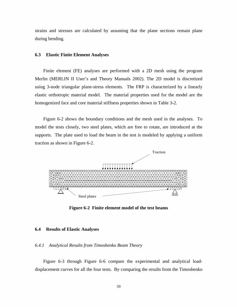
Tractions
Steel plates
strains and stresses are calculated by assuming that the plane sections remain plane
during bending.
6.3 Elastic Finite Element Analyses
Finite element (FE) analyses are performed with a 2D mesh using the program
Merlin (MERLIN II User’s and Theory Manuals 2002). The 2D model is discretized
using 3-node triangular plane-stress elements. The FRP is characterized by a linearly
elastic orthotropic material model. The material properties used for the model are the
homogenized face and core material stiffness properties shown in Table 3-2.
Figure 6-2 shows the boundary conditions and the mesh used in the analyses. To
model the tests closely, two steel plates, which are free to rotate, are introduced at the
supports. The plate used to load the beam in the test is modeled by applying a uniform
traction as shown in Figure 6-2.
Steel plates
Traction
Figure 6-2 Finite element model of the test beams
6.4 Results of Elastic Analyses
6.4.1 Analytical Results from Timoshenko Beam Theory
Figure 6-3 through Figure 6-6 compare the experimental and analytical load-
displacement curves for all the four tests. By comparing the results from the Timoshenko
59
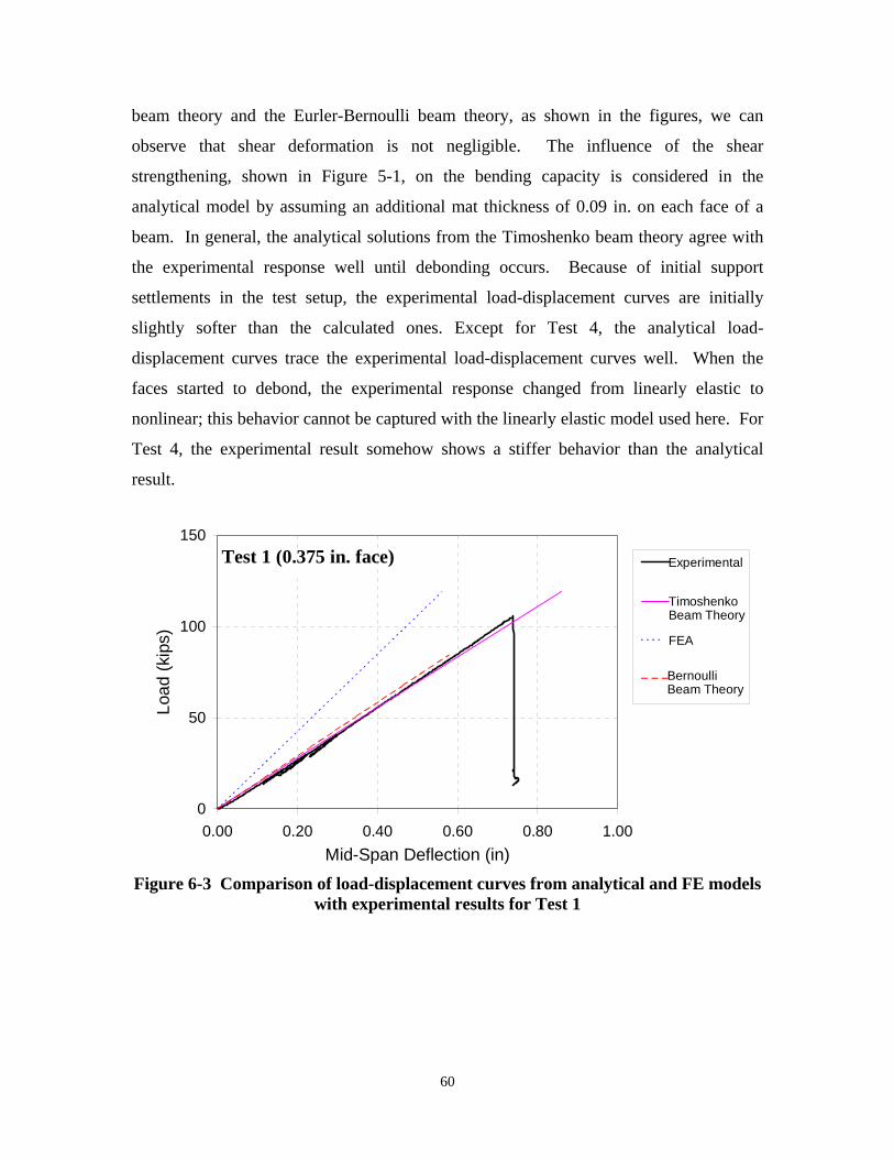
Experimental
TimoshenkoBeam theory
BernoulliBeam theory
FEA
0.375 - test1
beam theory and the Eurler-Bernoulli beam theory, as shown in the figures, we can
observe that shear deformation is not negligible. The influence of the shear Lo
ad (k
ips)
strengthening, shown in Figure 5-1, on the bending capacity is considered in the
analytical model by assuming an additional mat thickness of 0.09 in. on each face of a
beam. In general, the analytical solutions from the Timoshenko beam theory agree with
the experimental response well until debonding occurs. Because of initial support
settlements in the test setup, the experimental load-displacement curves are initially
slightly softer than the calculated ones. Except for Test 4, the analytical load-
displacement curves trace the experimental load-displacement curves well. When the
faces started to debond, the experimental response changed from linearly elastic to
nonlinear; this behavior cannot be captured with the linearly elastic model used here. For
Test 4, the experimental result somehow shows a stiffer behavior than the analytical
result.
150
100
50
0
Ti
)
lli
Experimental
moshenko Beam Theory
Test 1 (0.375 in. face
FEA
BernouBeam Theory
0.00 0.20 0.40 0.60 0.80 1.00 Mid-Span Deflection (in)
Figure 6-3 Comparison of load-displacement curves from analytical and FE models with experimental results for Test 1
60
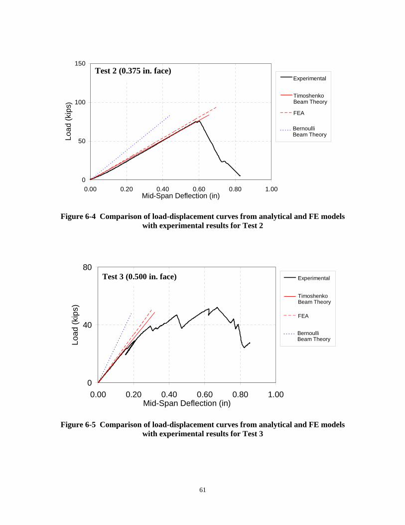
Experimental
TimoshenkoBeam theory
FEA
Bernoulli Beamtheory
0.375 - test2
Experimental
TimoshenkoBeam theory
FEA
Bernoulli Beamtheory
0.500 - test3
0
50
(ki
) )
Ti100
150 Lo
adps
Test 2 (0.375 in. faceExperimental
moshenko Beam Theory
FEA
Bernoulli Beam Theory
0.00 0.20 0.40 0.60 0.80 1.00Mid-Span Deflection (in)
Figure 6-4 Comparison of load-displacement curves from analytical and FE models with experimental results for Test 2
0
40
80
li
Load
(kip
s)
Test 3 (0.500 in. face) Experimental
Timoshenko Beam Theory
FEA
BernoulBeam Theory
0.00 0.20 0.40 0.60 0.80 1.00 Mid-Span Deflection (in)
Figure 6-5 Comparison of load-displacement curves from analytical and FE models with experimental results for Test 3
61
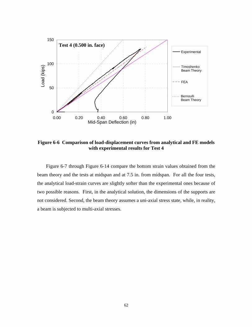
Experimental
Timoshenko Beamtheory
FEA
Bernoulli Beamtheory
0.500 - test4150
Load
(kip
s)
100
50
0
) i l
Ti
lli
Test 4 (0.500 in. faceExper menta
moshenko Beam Theory
FEA
BernouBeam Theory
0.00 0.20 0.40 0.60 0.80 1.00Mid-Span Deflection (in)
Figure 6-6 Comparison of load-displacement curves from analytical and FE models with experimental results for Test 4
Figure 6-7 through Figure 6-14 compare the bottom strain values obtained from the
beam theory and the tests at midspan and at 7.5 in. from midspan. For all the four tests,
the analytical load-strain curves are slightly softer than the experimental ones because of
two possible reasons. First, in the analytical solution, the dimensions of the supports are
not considered. Second, the beam theory assumes a uni-axial stress state, while, in reality,
a beam is subjected to multi-axial stresses.
62
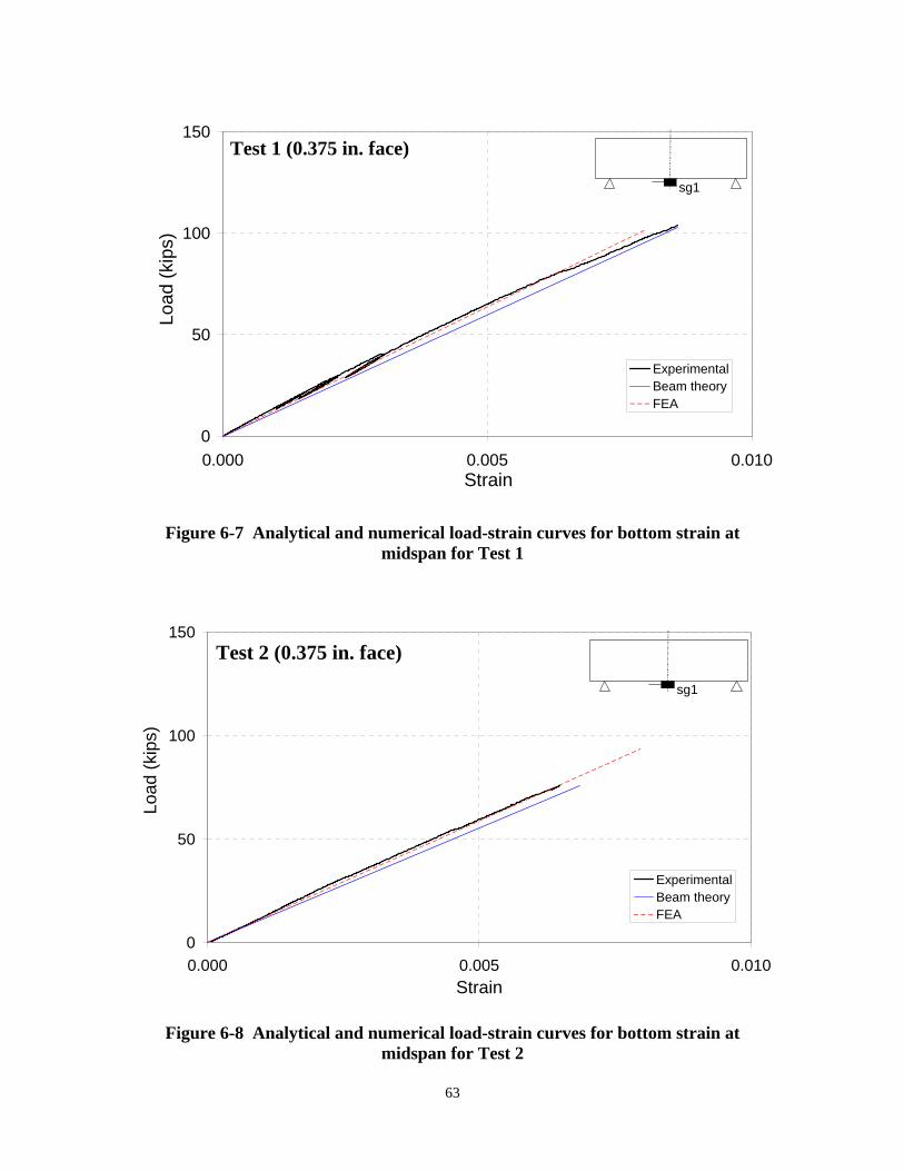
0
50
Load
(kip
s)
FEA
sg1
Test 1 (0.375 in. face)
100
150
Experimental Beam theory
0.000 0.005 0.010 Strain
Figure 6-7 Analytical and numerical load-strain curves for bottom strain at midspan for Test 1
0
50
Load
(kip
s)
FEA
sg1
Test 2 (0.375 in. face)
100
150
Experimental Beam theory
0.000 0.005 0.010 Strain
Figure 6-8 Analytical and numerical load-strain curves for bottom strain at midspan for Test 2
63

150 Lo
ad (k
ips)
FEA
sg1
Test 3 (0.500 in. face)
100
Experimental Beam theory
50
0 0.000 0.005 0.010
Strain
Figure 6-9 Analytical and numerical load-strain curves for bottom strain at midspan for Test 3
0
50
Load
(kip
s)
FEA
Test 4 (0.500 in. face)
100
150
Experimental Beam theory
sg1
0.000 0.005 0.010 Strain
Figure 6-10 Analytical and numerical load-strain curves for bottom strain at midspan for Test 4
64

Figure 6-11 through Figure 6-14 compare the load-strain curves obtained from the
analytical model and the tests for the bottom gage at 7.5 in. from midspan. Comparing
Figure 6-11 with Figure 6-12, it is evident that the experimental load-strain curves from
Test 1 and Test 2 are quite different. This is likely due to the malfunctioning of the gage
in Test 2, which resulted in the experimental load-strain curve in Figure 6-12 much stiffer
than the analytical result.
0
50
100
150
Load
(kip
s)
Test 1 (0.375 in. face)
Experimental Beam theory
sg5
0.000 0.005 0.010 Strain
Figure 6-11 Analytical and numerical load-strain curves for bottom strain at 7.5 in. from midspan for Test 1
65
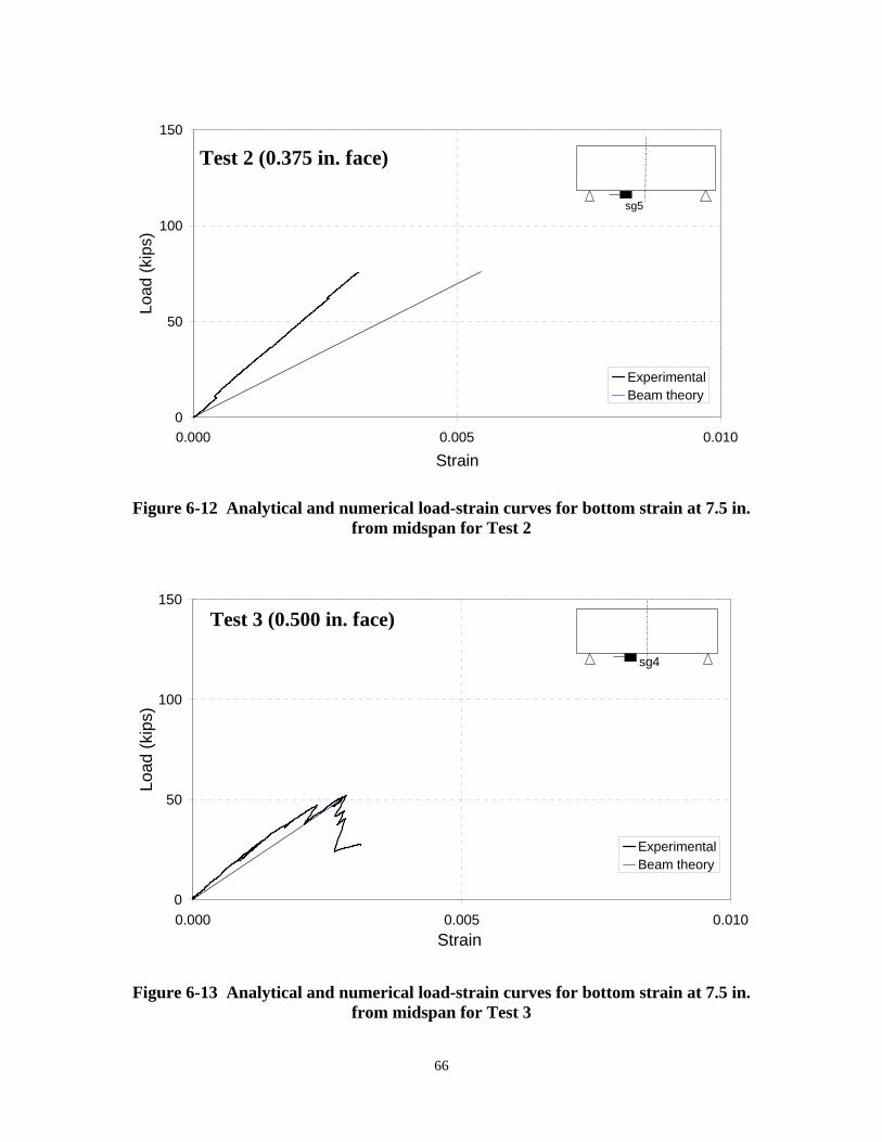
0
50
Load
(kip
s)
sg5
Test 2 (0.375 in. face)
100
150
Experimental Beam theory
0.000 0.005 0.010
Strain
Figure 6-12 Analytical and numerical load-strain curves for bottom strain at 7.5 in. from midspan for Test 2
0
50
Load
(kip
s)
Test 3 (0.500 in. face)
100
150
Experimental Beam theory
sg4
0.000 0.005
Strain
Figure 6-13 Analytical and numerical load-strain curves for bottom strain at 7.5 in. from midspan for Test 3
66
0.010
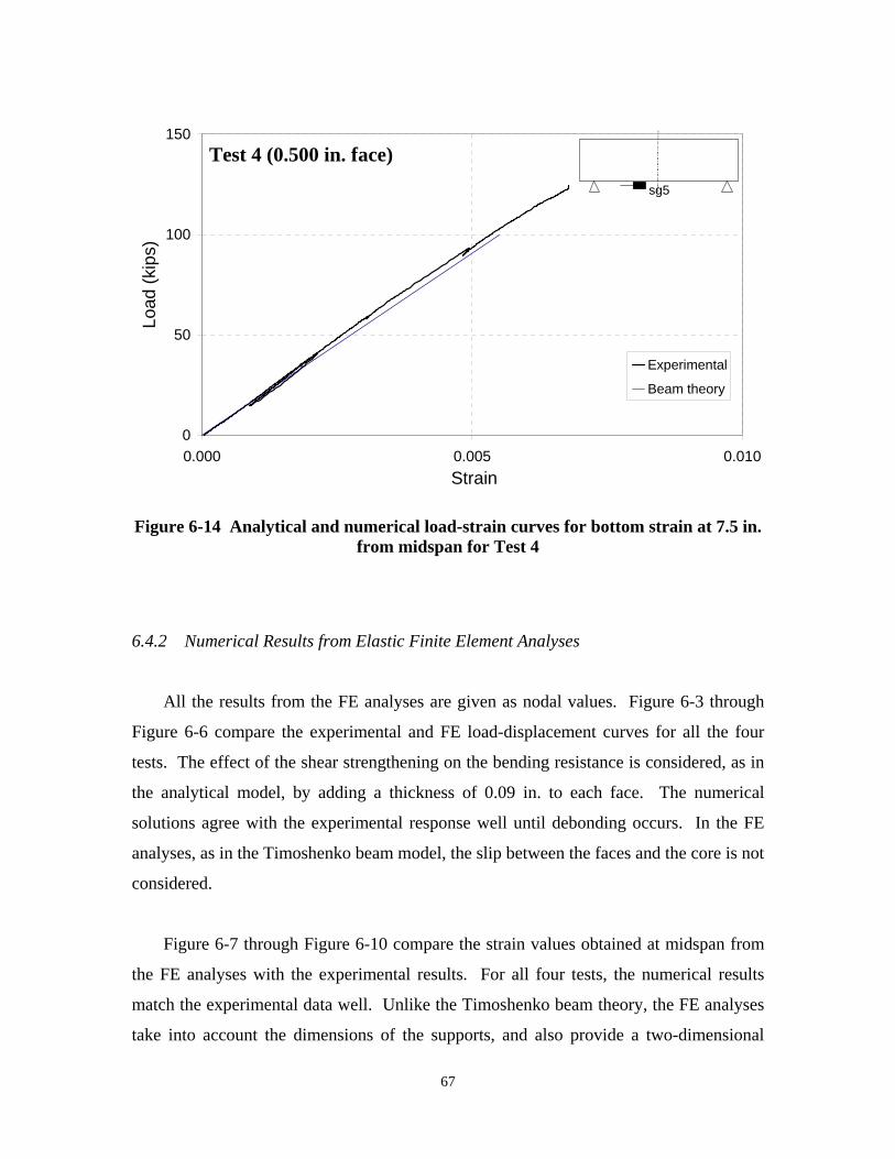
150 Lo
ad (k
ips)
100
50
0 0.000 0.005 0.010
Strain
i
Test 4 (0.500 in. face)
Exper mental
Beam theory
sg5
Figure 6-14 Analytical and numerical load-strain curves for bottom strain at 7.5 in. from midspan for Test 4
6.4.2 Numerical Results from Elastic Finite Element Analyses
All the results from the FE analyses are given as nodal values. Figure 6-3 through
Figure 6-6 compare the experimental and FE load-displacement curves for all the four
tests. The effect of the shear strengthening on the bending resistance is considered, as in
the analytical model, by adding a thickness of 0.09 in. to each face. The numerical
solutions agree with the experimental response well until debonding occurs. In the FE
analyses, as in the Timoshenko beam model, the slip between the faces and the core is not
considered.
Figure 6-7 through Figure 6-10 compare the strain values obtained at midspan from
the FE analyses with the experimental results. For all four tests, the numerical results
match the experimental data well. Unlike the Timoshenko beam theory, the FE analyses
take into account the dimensions of the supports, and also provide a two-dimensional
67
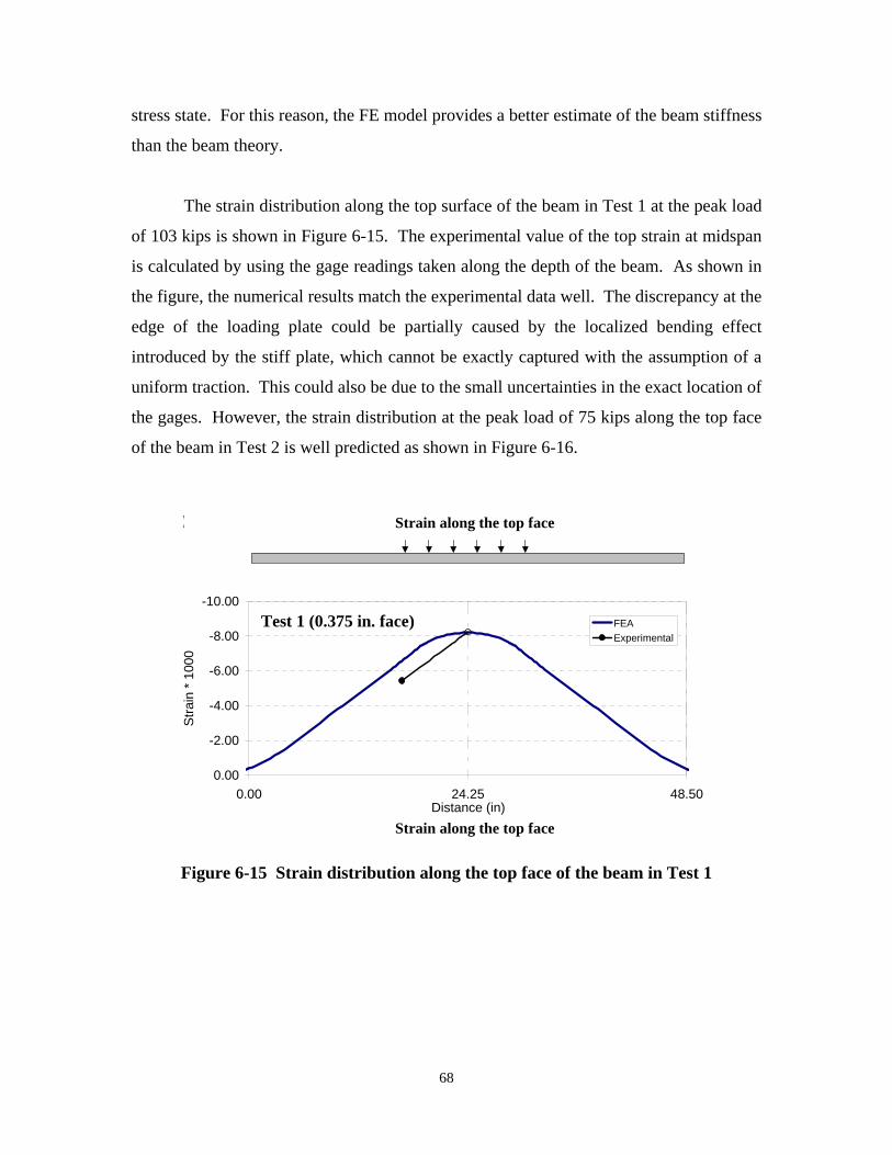
Strains along the top surface0.375 - test1
stress state. For this reason, the FE model provides a better estimate of the beam stiffness
than the beam theory.
The strain distribution along the top surface of the beam in Test 1 at the peak load
of 103 kips is shown in Figure 6-15. The experimental value of the top strain at midspan
is calculated by using the gage readings taken along the depth of the beam. As shown in
the figure, the numerical results match the experimental data well. The discrepancy at the
edge of the loading plate could be partially caused by the localized bending effect
introduced by the stiff plate, which cannot be exactly captured with the assumption of a
uniform traction. This could also be due to the small uncertainties in the exact location of
the gages. However, the strain distribution at the peak load of 75 kips along the top face
of the beam in Test 2 is well predicted as shown in Figure 6-16.
Strain along the top face
-8.00
-6.00
-4.00
-2.00
Stra
in *
100
0
FEA l
-10.00
0.00
ExperimentaTest 1 (0.375 in. face)
0.00 24.25 48.50 Distance (in)
Strain along the top face
Figure 6-15 Strain distribution along the top face of the beam in Test 1
68

0.375 - test2 Strain along the top surface
Stra
in *
100
0 -8.00
-6.00
-4.00
-2.00
0.00
) FEA Experimental
Test 2 (0.375 in. face
0.00 24.25 48.50 Distance (in)
Figure 6-16 Strain distribution along the top face of the beam in Test 2
In the third test, the face debonded early as the load increased. The face started to
debond at 23 kips. Below this load level, the FE analysis agrees with the experiment well
as shown for a load of 16 kips in Figure 6-17. This was a stage when the beam was still
acting as a full composite. After delamination, the difference between the FE analysis
and test results increases as shown for a load of 48 kips in Figure 6-17. This is due to the
loss of the composite action. The experimental strain in the face is smaller than the
calculated value because of the face slip. Furthermore, Figure 6-17 shows that at a load
of 48 kips, the experimental strain in the bottom face is larger than that in the top face.
This indicates that the top face had more severe debonding than the bottom face,
probably due to the localized bending effect caused by the steel loading plate.
69
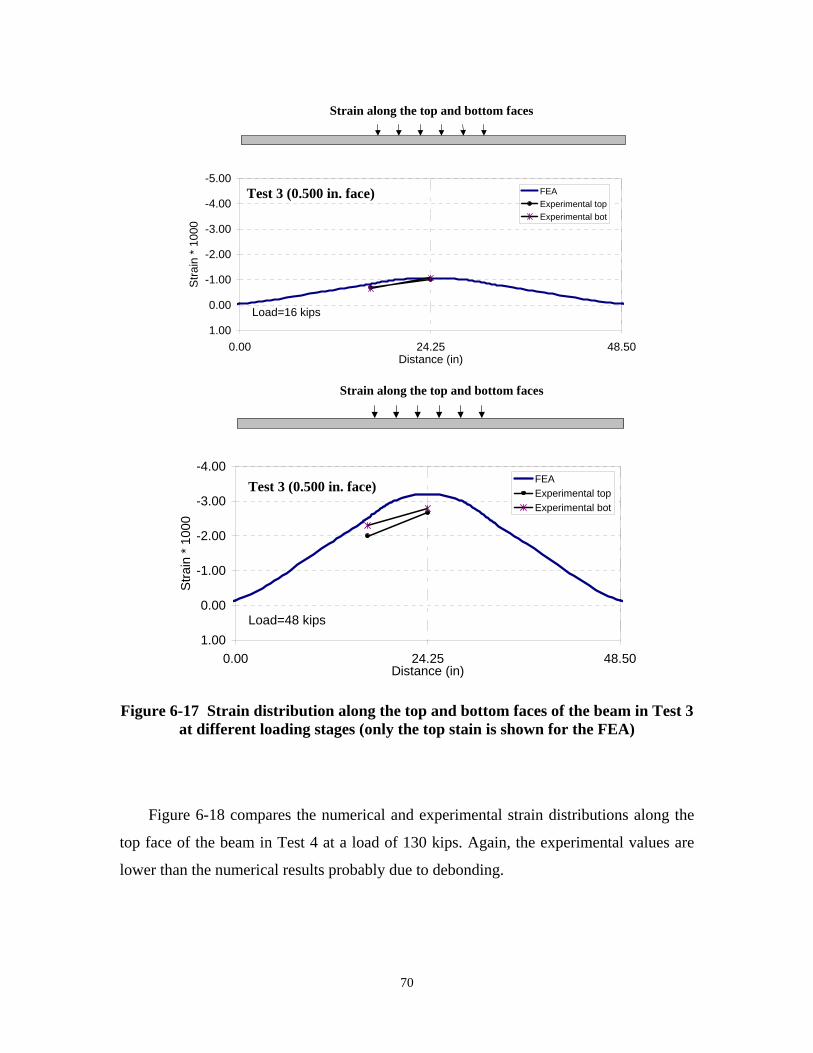
Strains along the top-bottom surface0.500 - test3
Strains along the top-bottom surface0.500 - test3
Strain along the top and bottom faces
Stra
in *
100
0 FEA
Load=16 kips
Test 3 ( ) -5.00
-4.00
-3.00
-2.00
-1.00
0.00
1.00
Experimental top Experimental bot
0.500 in. face
0.00 24.25 48.50 Distance (in)
Strain along the top and bottom faces
-4.00
-3.00
-2.00
-1.00
0.00
1.00
Stra
in *
100
0
FEA l top l bot
ips
( ) ExperimentaExperimenta
Load=48 k
Test 3 0.500 in. face
0.00 24.25 48.50 Distance (in)
Figure 6-17 Strain distribution along the top and bottom faces of the beam in Test 3 at different loading stages (only the top stain is shown for the FEA)
Figure 6-18 compares the numerical and experimental strain distributions along the
top face of the beam in Test 4 at a load of 130 kips. Again, the experimental values are
lower than the numerical results probably due to debonding.
70
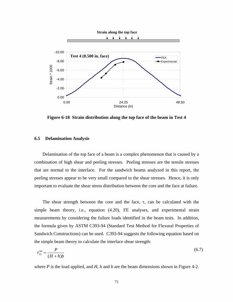
Strains along the top interface0.500 - test4 Strain along the top face
Stra
in *
100
0 -10.00
-8.00
-6.00
-4.00
-2.00
0.00
FEA Experimental
( )Test 4 0.500 in. face
0.00 24.25 48.50 Distance (in)
Figure 6-18 Strain distribution along the top face of the beam in Test 4
6.5 Delamination Analysis
Delamination of the top face of a beam is a complex phenomenon that is caused by a
combination of high shear and peeling stresses. Peeling stresses are the tensile stresses
that are normal to the interface. For the sandwich beams analyzed in this report, the
peeling stresses appear to be very small compared to the shear stresses. Hence, it is only
important to evaluate the shear stress distribution between the core and the face at failure.
The shear strength between the core and the face, τ, can be calculated with the
simple beam theory, i.e., equation (4.20), FE analyses, and experimental strain
measurements by considering the failure loads identified in the beam tests. In addition,
the formula given by ASTM C393-94 (Standard Test Method for Flexural Properties of
Sandwich Constructions) can be used. C393-94 suggests the following equation based on
the simple beam theory to calculate the interface shear strength:
τ int = P (6.7)
13 (H h b + )
where P is the load applied, and H, h and b are the beam dimensions shown in Figure 4-2.
71
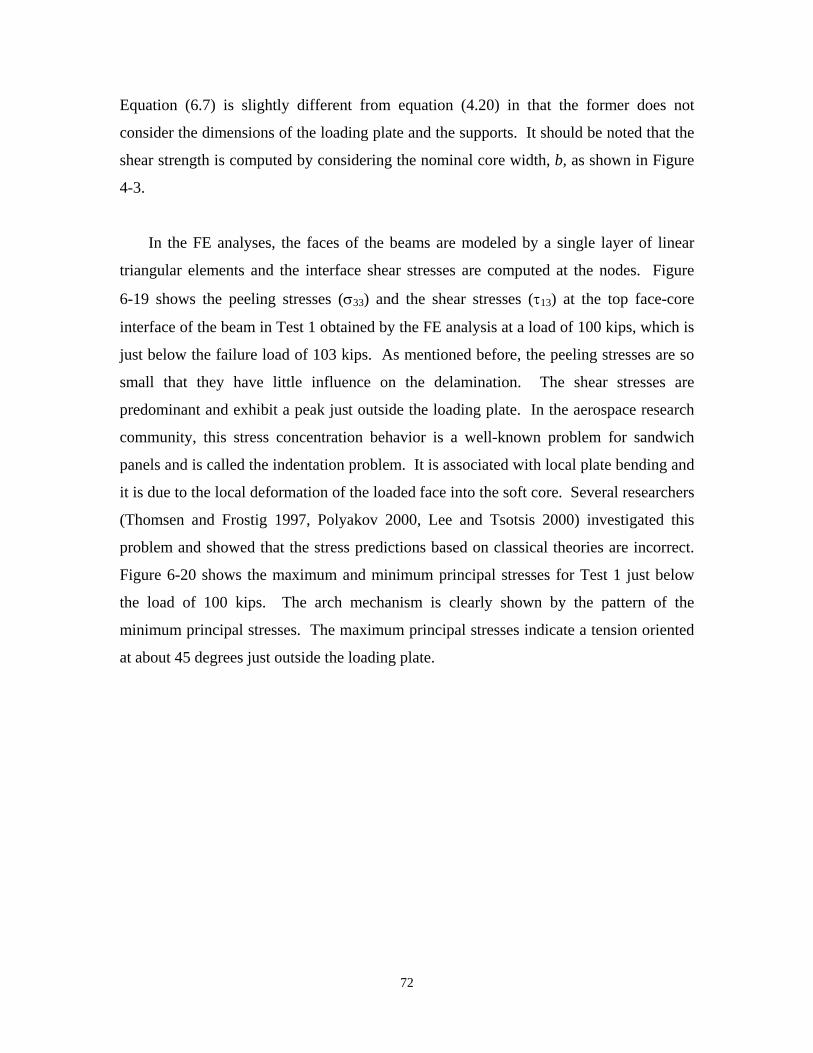
Equation (6.7) is slightly different from equation (4.20) in that the former does not
consider the dimensions of the loading plate and the supports. It should be noted that the
shear strength is computed by considering the nominal core width, b, as shown in Figure
4-3.
In the FE analyses, the faces of the beams are modeled by a single layer of linear
triangular elements and the interface shear stresses are computed at the nodes. Figure
6-19 shows the peeling stresses (σ33) and the shear stresses (τ13) at the top face-core
interface of the beam in Test 1 obtained by the FE analysis at a load of 100 kips, which is
just below the failure load of 103 kips. As mentioned before, the peeling stresses are so
small that they have little influence on the delamination. The shear stresses are
predominant and exhibit a peak just outside the loading plate. In the aerospace research
community, this stress concentration behavior is a well-known problem for sandwich
panels and is called the indentation problem. It is associated with local plate bending and
it is due to the local deformation of the loaded face into the soft core. Several researchers
(Thomsen and Frostig 1997, Polyakov 2000, Lee and Tsotsis 2000) investigated this
problem and showed that the stress predictions based on classical theories are incorrect.
Figure 6-20 shows the maximum and minimum principal stresses for Test 1 just below
the load of 100 kips. The arch mechanism is clearly shown by the pattern of the
minimum principal stresses. The maximum principal stresses indicate a tension oriented
at about 45 degrees just outside the loading plate.
72

0.375 - test1
-0.8
-0.6
-0.4
-0.2
0.0
0.2
0.4
0.6
0.8 0.00
Stre
sses
alo
ng th
e to
p fa
ce/c
ore
inte
rfac
e (k
si)
24.25 Distance (in.)
48.50
τ13
σ33
)Test 1 (0.375 in. face
Figure 6-19 Stresses along the interface between the top face and the core of the beam in Test 1 from FE analysis
Plate
Plate
Principal stresses - M inim um
Principal stresses - M axim um
Figure 6-20 Maximum and minimum principal stresses for Test 1 from FE analysis
By considering a schematic similar to that shown in Figure 4-3, the interface shear
stress can be estimated from the experimental strain readings in the following way. The
resultant bending force in the top face of a beam can be estimated from the strain gage
73
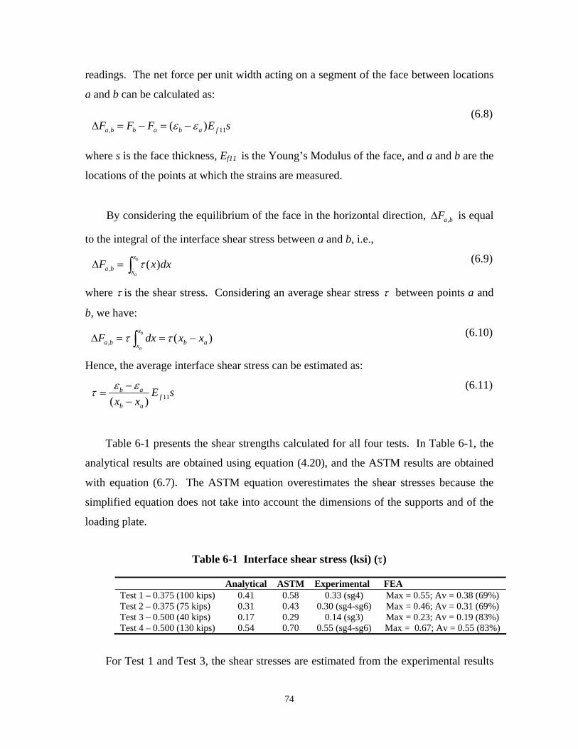
readings. The net force per unit width acting on a segment of the face between locations
a and b can be calculated as:
(6.8)∆Fa b = F − F = (ε − ε )E s , b a b a f 11
where s is the face thickness, Ef11 is the Young’s Modulus of the face, and a and b are the
locations of the points at which the strains are measured.
By considering the equilibrium of the face in the horizontal direction, ∆Fa b is equal ,
to the integral of the interface shear stress between a and b, i.e.,
( ) (6.9)∆Fa b = ∫x
x
a
b τ x dx ,
where τ is the shear stress. Considering an average shear stress τ between points a and
b, we have:
(6.10)∆Fa b = τ ∫x
x
a
b dx = τ ( x − x ), b a
Hence, the average interface shear stress can be estimated as:
εb − ε (6.11)τ = a E s
( x − x ) f 11b a
Table 6-1 presents the shear strengths calculated for all four tests. In Table 6-1, the
analytical results are obtained using equation (4.20), and the ASTM results are obtained
with equation (6.7). The ASTM equation overestimates the shear stresses because the
simplified equation does not take into account the dimensions of the supports and of the
loading plate.
Table 6-1 Interface shear stress (ksi) (τ)
Analytical ASTM Experimental FEA Test 1 – 0.375 (100 kips) 0.41 0.58 0.33 (sg4) Max = 0.55; Av = 0.38 (69%) Test 2 – 0.375 (75 kips) 0.31 0.43 0.30 (sg4-sg6) Max = 0.46; Av = 0.31 (69%) Test 3 – 0.500 (40 kips) 0.17 0.29 0.14 (sg3) Max = 0.23; Av = 0.19 (83%) Test 4 – 0.500 (130 kips) 0.54 0.70 0.55 (sg4-sg6) Max = 0.67; Av = 0.55 (83%)
For Test 1 and Test 3, the shear stresses are estimated from the experimental results
74

with a single gage (sg4) reading by considering the equilibrium of the top face over a
distance x = xb - xa, where xa is at a free end of the beam as shown in Figure 6-21. For
Test 2 and Test 4, the results are obtained by using the readings of the two gages
indicated in Table 6-1. Only Test 2 and Test 4 had both sg6 and sg4 gages glued on the
top of the beams in the shear span region, where the shear stress is almost constant.
x
Supports
τ
48.5 in. xa xb
Loading plate
0 in.
Figure 6-21 Average shear stress
The FE results presented in Table 6-1 show both the maximum shear stress values
calculated and the average shear stresses calculated over the distance, x. The average
stresses are calculated to compare the FE results to the experimental and analytical
results. For the beams with 0.375- and 0.500-in. faces, the average shear stress is 69 %
and 83% of the maximum shear stress, respectively. This means that by increasing the
face thickness, we can minimize the localized bending effect induced by the loading
plate.
The interface shear strengths obtained in this study are compared to that of prior
studies (Stone et al. 2001 and Lopez 2001) in Table 6-2. Beams in the prior studies did
not have the shear strengthening used in this study (see Figure 2-2).
75

Table 6-2 Comparison of the interface shear strengths (ksi) with and without shear strengthening
Without shear With shear strengthening strengthening
Analytical ASTM Analytical ASTM (Eq. (4.20)) (Eq. (6.7)) (Eq. (4.20)) (Eq. (6.7))
Stone 1 (2001) 0.14 0.19 Test 1 - 0.375 0.41 0.58 Stone 2 (2001) 0.21 0.28 Test 2 - 0.375 0.31 0.43 Lopez 1 (2001) 0.08 0.10 Test 3 - 0.500 0.16 0.29 Lopez 1 (2001) 0.085 0.15 Test 4 - 0.500 0.54 0.70
Average 0.13 0.18 Average 0.36 0.50
For short spans, the ASTM results overestimate the shear strengths and they are
shown here only for completeness. The results show that the new shear strengthening
detail increased the average shear strength by 2.8 times. In this study, the lowest shear
strength value was found in Test 3, which failed in a ductile-like manner because of
possible defects in the interface. This and prior studies have shown that the bonding
between the faces and the core is the most important parameter governing the bending
capacity of a panel. Quality control is important for all engineering materials but is
especially critical for composite materials. It is therefore essential that the manufacturing
process assures a good quality control of the face-core interface.
6.6 Nonlinear Fracture Mechanics Analysis of the Face-Core Interface
The delamination failure is studied by using a Nonlinear Fracture Mechanics
(NLFM) model developed at the University of Colorado (Cervenka et al. 1998) and
implemented in an interface element in the program Merlin (MERLIN II User’s and
Theory Manuals 2002). The discrete crack model used is a generalization of the classical
Fictitious Crack Model of Hillerborg et al. (1976), modified to account for the shear
effects along the fracture process zone (FPZ) and the crack. In this model, the interface
strength is described by the following failure function (Cervenka et al. 1998): 2 2 2 2 2F = (τ +τ ) − 2cTan(φ )(σ − σ ) − Tan (φ )(σ −σ f ) = 0 (6.12)1 2 f t f
where c is the cohesion, φf is the angle of friction, σt is the interface tensile strength, τ1
and τ2 are the two tangential components of the interface traction vector, and σ is the
76
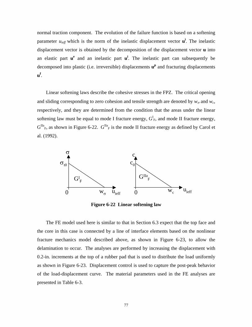
normal traction component. The evolution of the failure function is based on a softening
parameter uieff which is the norm of the inelastic displacement vector ui. The inelastic
displacement vector is obtained by the decomposition of the displacement vector u into ean elastic part u and an inelastic part ui. The inelastic part can subsequently be
decomposed into plastic (i.e. irreversible) displacements up and fracturing displacements fu .
Linear softening laws describe the cohesive stresses in the FPZ. The critical opening
and sliding corresponding to zero cohesion and tensile strength are denoted by wσ and wc,
respectively, and they are determined from the condition that the areas under the linear
softening law must be equal to mode I fracture energy, GIF, and mode II fracture energy,
GIIa F, as shown in Figure 6-22. GIIa
F is the mode II fracture energy as defined by Carol et
al. (1992).
σ
cc 0σt0
GIIa FGI
F
0 wσ uieff 0 wc uieff
Figure 6-22 Linear softening law
The FE model used here is similar to that in Section 6.3 expect that the top face and
the core in this case is connected by a line of interface elements based on the nonlinear
fracture mechanics model described above, as shown in Figure 6-23, to allow the
delamination to occur. The analyses are performed by increasing the displacement with
0.2-in. increments at the top of a rubber pad that is used to distribute the load uniformly
as shown in Figure 6-23. Displacement control is used to capture the post-peak behavior
of the load-displacement curve. The material parameters used in the FE analyses are
presented in Table 6-3.
77

Imposed displacement
Interface crack Rubber pad
Figure 6-23 Finite element mesh for nonlinear fracture mechanics analysis
Table 6-3 Interface material parameters
Interface parameters Shear Stiffness Kt 284000 psi/in. (assumed) Normal Stiffness Kn 284000 psi/in. (assumed) Tensile Strength σt0 380 psi (glue tensile strength from manufacturer)Cohesion c 550 psi (result from Test 1) Friction Angle φf 53 degrees Dilatancy Angle φt 45 degrees Specific mode I fracture energy GI
F 0.1 lbf/in. Specific mode II fracture energy GIIa
F 1.0 lbf/in. Ratio of irreversible displacement γ 0.3 Maximum dilatant displacement umax 0.4 in
The cohesion value is selected to match the result of Test 1. The interface specific
mode I fracture energy, GIF, is based on tests conducted on similar sandwich panels by
Smith (2001). The mode II fracture energy, GIIaF, is assumed to be 10 times GI
F. The
interface normal stiffness is chosen to be the highest possible value that provides a well
conditioned numerical solution. The interface shear stiffness is assumed to be equal to
the interface normal stiffness. Since the face-core interface normally exhibits a brittle
fracture behavior, the friction angle φf, the dilatancy angle φt, ratio of irreversible
displacement γ, and the maximum dilatant displacement umax do not influence the
numerical results too much. Hence, their values are arbitrarily selected. The analysis
results are shown in Figure 6-24. The analysis of Test 1 shows an excellent agreement
with the experimental result. This is expected as the model is calibrated to match this
test. However, for Test 2 and Test 4 numerical peak loads are 21.5% higher and 28%
78

0.500 - test4
0.375 - test1 0.375 - test2
0.500 - test3
lower than the experimental results, respectively. This is because the same fracture
properties are used in all the analyses and the interface strengths are different in different
test beams as shown in Table 6-1. Similarly, the fracture parameters used do not trace
Test 3 accurately. The numerical failure load for Test 3 is 2.66 times the experimental
result. As already said, the premature failure in the test was caused by the fact that the
top face was not glued to the core with a uniform quality. This reduced the interface
shear strength and triggered the premature failure. It is expected that if the actual
interface shear strengths were used in the analyses, the numerical results would match the
experiments a lot better.
0
50
100
150
ips)
0
50
100
150
NLFM NLFM
i ) in. face)
Load
(k
Load
(kip
s)
Test 1 (0.375 n. face Test 2 (0.375
0.00 0.20 0.40 0.60 0.80 1.00 0.00 0.20 0.40 0.60 0.80 1.00 Mid-Span Deflection (in) Mid-Span Deflection (in)
0
50
ips)
0
50
100
150
i)
in. face) ( i
100
150
Load
(k
Load
(kps
NLFM
NLFM
Test 3 (0.500 Test 4 0.500 n. face)
0.00 0.20 0.40 0.60 0.80 1.00 0.00 0.20 0.40 0.60 0.80 1.00 Mid-Span Deflection (in) Mid-Span Deflection (in)
Figure 6-24 Finite element analysis results
Figure 6-25 shows the deformed shape at failure for Test 2. Debonding starts near
the edge of the loading plate (Figure 6-25 (a)), and propagates toward the end of the
79
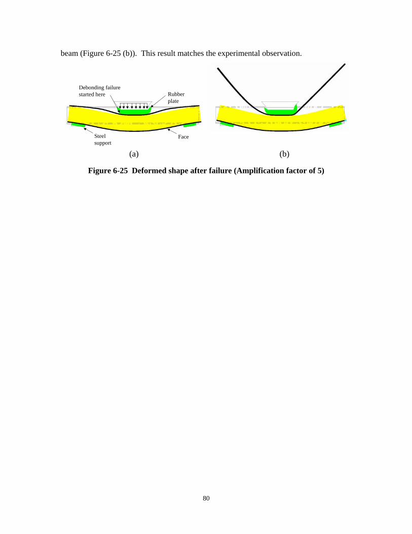
beam (Figure 6-25 (b)). This result matches the experimental observation.
Rubber Debonding failure started here
plate
Face Steel support
(a) (b)
Figure 6-25 Deformed shape after failure (Amplification factor of 5)
80
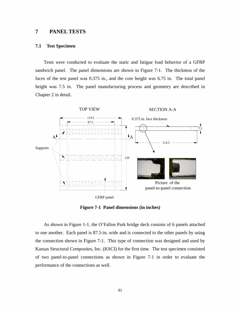
81
7 PANEL TESTS EQUATION CHAPTER 7 SECTION 1 7.1 Test Specimen
Tests were conducted to evaluate the static and fatigue load behavior of a GFRP
sandwich panel. The panel dimensions are shown in Figure 7-1. The thickness of the
faces of the test panel was 0.375 in., and the core height was 6.75 in. The total panel
height was 7.5 in. The panel manufacturing process and geometry are described in
Chapter 2 in detail.
SECTION A-A
AA
TOP VIEW
Picture of thepanel-to-panel connection
Supports
GFRP panel
0.375 in. face thickness
7.5
114.5
120
87.5114.5
Figure 7-1 Panel dimensions (in inches)
As shown in Figure 1-1, the O’Fallon Park bridge deck consists of 6 panels attached
to one another. Each panel is 87.5-in. wide and is connected to the other panels by using
the connection shown in Figure 7-1. This type of connection was designed and used by
Kansas Structural Composites, Inc. (KSCI) for the first time. The test specimen consisted
of two panel-to-panel connections as shown in Figure 7-1 in order to evaluate the
performance of the connections as well.
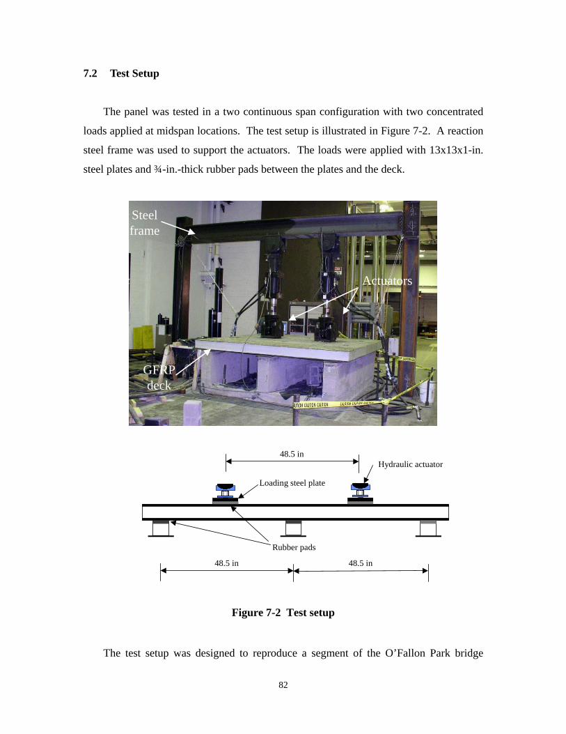
7.2 Test Setup
The panel was tested in a two continuous span configuration with two concentrated
loads applied at midspan locations. The test setup is illustrated in Figure 7-2. A reaction
steel frame was used to support the actuators. The loads were applied with 13x13x1-in.
steel plates and ¾-in.-thick rubber pads between the plates and the deck.
Steel
GFRP deck
48.5 in
Loading steel plate
48.5 in
Hydraulic actuator
Rubber pads
Actuators
frame
48.5 in
Figure 7-2 Test setup
The test setup was designed to reproduce a segment of the O’Fallon Park bridge
82
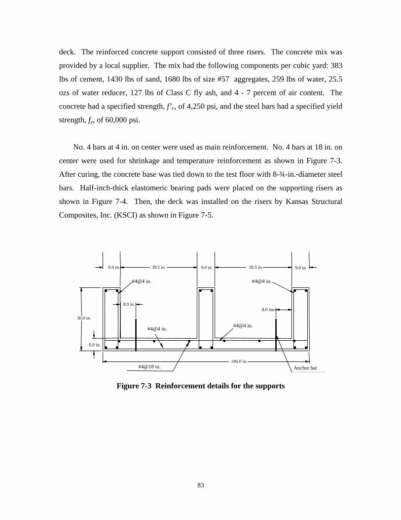
deck. The reinforced concrete support consisted of three risers. The concrete mix was
provided by a local supplier. The mix had the following components per cubic yard: 383
lbs of cement, 1430 lbs of sand, 1680 lbs of size #57 aggregates, 259 lbs of water, 25.5
ozs of water reducer, 127 lbs of Class C fly ash, and 4 - 7 percent of air content. The
concrete had a specified strength, f’c, of 4,250 psi, and the steel bars had a specified yield
strength, fy, of 60,000 psi.
No. 4 bars at 4 in. on center were used as main reinforcement. No. 4 bars at 18 in. on
center were used for shrinkage and temperature reinforcement as shown in Figure 7-3.
After curing, the concrete base was tied down to the test floor with 8-¾-in.-diameter steel
bars. Half-inch-thick elastomeric bearing pads were placed on the supporting risers as
shown in Figure 7-4. Then, the deck was installed on the risers by Kansas Structural
Composites, Inc. (KSCI) as shown in Figure 7-5.
30.0 in.
106.0 in.
6.0 in.
39.5 in. 9.0 in.
8.0 in. 8.0 in.
#4@4 in.
#4@18 in. Anchor bar
#4@4 in.
#4@4 in. #4@4 in.
9.0 in. 39.5 in. 9.0 in.
Figure 7-3 Reinforcement details for the supports
83
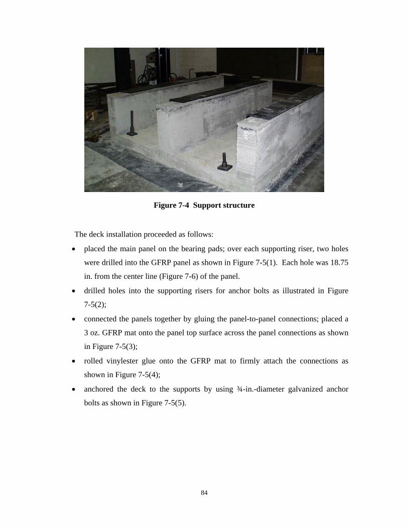
Figure 7-4 Support structure
The deck installation proceeded as follows:
• placed the main panel on the bearing pads; over each supporting riser, two holes
were drilled into the GFRP panel as shown in Figure 7-5(1). Each hole was 18.75
in. from the center line (Figure 7-6) of the panel.
• drilled holes into the supporting risers for anchor bolts as illustrated in Figure
7-5(2);
• connected the panels together by gluing the panel-to-panel connections; placed a
3 oz. GFRP mat onto the panel top surface across the panel connections as shown
in Figure 7-5(3);
• rolled vinylester glue onto the GFRP mat to firmly attach the connections as
shown in Figure 7-5(4);
• anchored the deck to the supports by using ¾-in.-diameter galvanized anchor
bolts as shown in Figure 7-5(5).
84
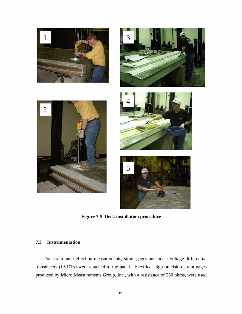
1
2
3
4
5
Figure 7-5 Deck installation procedure
7.3 Instrumentation
For strain and deflection measurements, strain gages and linear voltage differential
transducers (LVDTs) were attached to the panel. Electrical high precision strain gages
produced by Micro Measurements Group, Inc., with a resistance of 350 ohms, were used
85

along with M-Bond Type AE 10 adhesive system to measure strains. Deflection was
monitored using LVDTs. Displacement and strain readings, as well as the load and
stroke of the actuators, were recorded during the tests by using a 48-channels data-
acquisition system. Figure 7-6 provides a schematic of the strain gage locations and
Figure 7-7 indicates the LVDT positions on the panel. For the following discussion, the
span on the north side is called Span 1, and the span on the south side is called Span 2, as
shown in Figure 7-7.
7.4 Test Procedure
The objective of the tests was to evaluate the load carrying capacity of the GFRP
deck panel under static and fatigue loads. The tests were divided into five loading phases
as shown in Table 7-1. In Table 7-1, Actuator 1 was used to load Span 1 and Actuator 2
was used to load Span 2. Data were recorded at different loading phases to evaluate the
structural performance of the panel as shown in Table 7-2
Table 7-1 Loading stages
Initial Static Test
Phase 1 – Cyclic Phase 2 - Cyclic Phase 3 - Cyclic Final Static Test
Load cycles 0
0 - 15,200 15,200-370,200 370,200 to 1,500,000 1,500,000
Loading configuration Both spans loaded at the same time Actuators 1 and 2 180º off phase Actuator 1 Actuator 1 Actuator 1 and then 2
Table 7-2 Data recorded
Load cycle No. Loading configuration Initial Static Test 0 Both spans loaded at the same
time Cyclic data 1 15,000-15,200 Actuators 1 and 2 180º off phase Cyclic data 2 370,000-370,200 Actuator 1 Static test 1M 1,000,000 Actuator 1 Static test 1.5M 1,500,000 Actuator 1 Final Static Test 1,500,000 Actuator 1 and then 2
86

B
CC 9
20
1 16
1 2
3 4 5
6
7
8
916
17
18
8.5
18.7518.75 1119.75 11.75
x1
x2
x3
9
20
19.75
10
12
13
14
1519 21
8.5
18.7518.75 1119.75
11
20
Span 2
CC
B
Span 2 Span 1
Top surface
Mid
span
2
Mid
span
1
Mid
span
2
Mid
span
1
Panel center line
Span 1
Panel center line
Bottom surface
Figure 7-6 Strain gage locations for the panel test (all dimensions in inches)
87
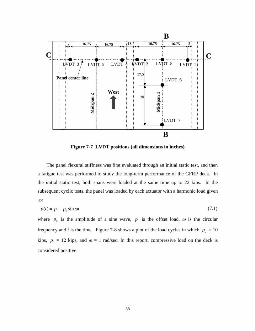
8
6
7
20
16.75
17.5
16.7516.75 1316.752 2
LVDT 124LVDT 53
B
CC
West
LVDT
LVDT
LVDT
Mid
span
2
Mid
span
1
LVDTLVDTLVDT
Panel center line
B
Figure 7-7 LVDT positions (all dimensions in inches)
The panel flexural stiffness was first evaluated through an initial static test, and then
a fatigue test was performed to study the long-term performance of the GFRP deck. In
the initial static test, both spans were loaded at the same time up to 22 kips. In the
subsequent cyclic tests, the panel was loaded by each actuator with a harmonic load given
as:
( )p t = ip + 0 sin p ωt (7.1)
where 0p is the amplitude of a sine wave, pi is the offset load, ω is the circular
frequency and t is the time. Figure 7-8 shows a plot of the load cycles in which p = 100
kips, pi = 12 kips, and ω = 1 rad/sec. In this report, compressive load on the deck is
considered positive.
88
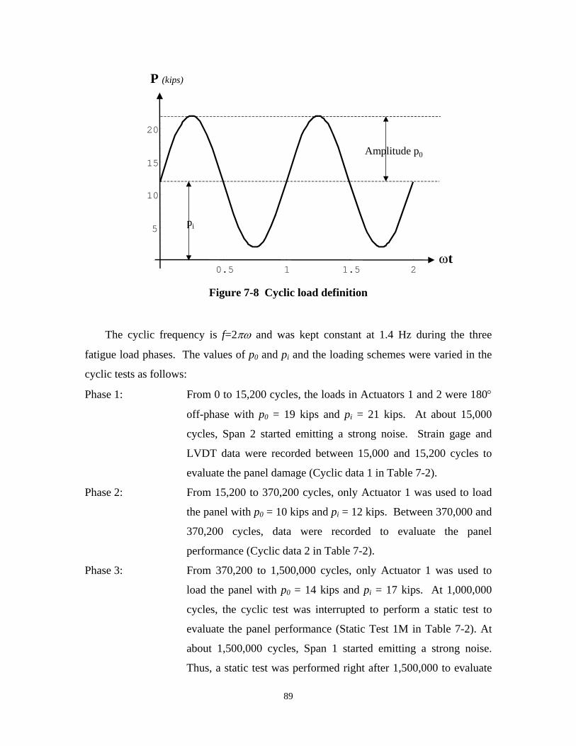
25P (kips)
20
0.5 1 1.5 2
5
0
pi
Amplitude p15
10
ω t
Figure 7-8 Cyclic load definition
The cyclic frequency is f=2πω and was kept constant at 1.4 Hz during the three
fatigue load phases. The values of p0 and pi and the loading schemes were varied in the
cyclic tests as follows:
Phase 1: From 0 to 15,200 cycles, the loads in Actuators 1 and 2 were 180°
off-phase with p0 = 19 kips and pi = 21 kips. At about 15,000
cycles, Span 2 started emitting a strong noise. Strain gage and
LVDT data were recorded between 15,000 and 15,200 cycles to
evaluate the panel damage (Cyclic data 1 in Table 7-2).
Phase 2: From 15,200 to 370,200 cycles, only Actuator 1 was used to load
the panel with p0 = 10 kips and pi = 12 kips. Between 370,000 and
370,200 cycles, data were recorded to evaluate the panel
performance (Cyclic data 2 in Table 7-2).
Phase 3: From 370,200 to 1,500,000 cycles, only Actuator 1 was used to
load the panel with p0 = 14 kips and pi = 17 kips. At 1,000,000
cycles, the cyclic test was interrupted to perform a static test to
evaluate the panel performance (Static Test 1M in Table 7-2). At
about 1,500,000 cycles, Span 1 started emitting a strong noise.
Thus, a static test was performed right after 1,500,000 to evaluate
89

the damage in the panel (Static Test 1.5M in Table 7-2).
At the end of the fatigue test, the two spans were loaded one at a time up to 100
kips, which is close to the loading capacity of the actuators used.
7.5 Initial Static Test
The purpose of the initial static test was to evaluate the flexural behavior of the
virgin panel. In this test, both spans were loaded at the same time up to 22 kips. Both
strain gage and LVDT data were obtained in this test. A schematic of the LVDT locations
along the center line of the panel (line C-C in Figure 7-7) is shown in Figure 7-9.
Load 2
R1 R2 R3
2 in.
LVDT3 LVDT5 LVDT4 LVDT2 LVDT8 LVDT1
2 in.
Bearing pads
Load 1
Figure 7-9 Elevation view of the LVDT locations
The panel stiffness was difficult to determine from the test results because it was
influenced by the settlement of the bearing pads. For this reason, one LVDT was placed
near each support to record the displacement due to the settlement of the bearing pads.
Figure 7-10 shows the experimental load-displacement curves from all the LVDTs placed
along line C-C shown in Figure 7-7.
90

Load Vs LVDTs
0
5
10
15
20
25 Lo
ad (k
ips)
1 2 34 8 5
Initial Static Test
0 -0.02 -0.04 -0.06 -0.08 -0.1 -0.12 -0.14
Displacement (in)
Figure 7-10 Load-displacement curves for the initial static test
The anchor bolts on riser R1 (see Figure 7-9) slipped during the test. Visual
inspection at the end of the static test showed that the bearing pad placed on riser R1
moved from the initial position. The pad rotated and left a gap between the riser and the
panel at the location of line C-C, and this explains why LVDT 3 registered a larger
deflection than LVDT 5. The deformed shape of the panel at 22 kips, drawn with
AUTOCAD 2000 using the LVDT readings, is shown in Figure 7-11. In this figure, a
Bezier curve is used to approximate the deformed shape and estimate the actual
deformation of the panel. A Bezier curve is a simple cubic equation and was originally
developed by Pierre Bézier in the 1970's for CAD applications. A cubic Bezier curve is
defined by four points: (x0,y0) is the origin point, and (x3,y3) is the destination point, and
(x1,y1) and (x2,y2) are control points.
Equations (7.2) and (7.3) are used to define the points on a Bezier curve. The points
on the curve are evaluated by varying the values of t between 0 and 1. One equation
91

yields values for x, and the other yields values for y.
x(t) = axt3 + bxt2 + cxt + x0 (7.2)
y(t) = ayt3 + byt2 + cyt + y0 (7.3)
where:
cx = 3 (x1 - x0) bx = 3 (x2 - x1) - cx ax = x3 - x0 - cx - bx
cy = 3 (y1 - y0) by = 3 (y2 - y1) - cy ay = y3 - y0 - cy - by
All dimensions in Figure 7-11 are in scale, with the displacements in the x3 direction
amplified 30 times. The curve is forced to have a horizontal tangent at the center of the
interior riser, R2, and it is used to estimate the bearing pad settlements at the supports.
LVDT 4 LVDT 8
0.124 0.041 0.066 0.041
0.042
0.074
0.75 x3,w
x1
LVDT 3 LVDT 5
0.114
LVDT 2
0.055
LVDT 1
¾ in. bearing rubber pads
Actual deflection of span 2 Actual deflection
of span 1
Figure 7-11 Deformed shape along line C-C (All dimensions in inches, deflections amplified 30 times)
The actual panel deflections at midspans are estimated with the deflection curve in
Figure 7-11 by taking out the rigid-body displacement due to the support settlements. As
shown in Figure 7-12, the load-vs-actual displacement curves for the two spans are much
stiffer than those obtained with the unadjusted readings from LVDT 5 and 8.
92

Load Vs Actual Deflection
0
5
10
15
20
25 Lo
ad (k
ips)
Initial Static Test
Mi
Midspan 2
dspan 1
0 -0.0125 -0.025 -0.0375 -0.05 Displacement (in)
Figure 7-12 Load-vs-actual deflection curves for the initial static test
From the load-displacement curves in Figure 7-12, we can see that the midspan
deflections under the service loads of 26 kips were 0.048 and 0.047 in. for Spans 1 and 2,
respectively. These satisfy the deflection limit of L/1000 (0.05 in.) specified in the
design provisions of the City and County of Denver.
Figure 7-13 shows the load-strain curves obtained from all the strain gages glued on
the panel. Loads 1 and 2 are defined in Figure 7-9. The curves are linear. As expected,
the strain decreases with increasing distance from line C-C (Figure 7-6). At 37.5 in. from
line C-C, the deformation is negligible. Figure 7-14 shows the strains ε along line B-B11
(Figure 7-6) obtained from the gages glued on the top and bottom of Span 1, where ε is
the longitudinal strain in direction x1 as defined in Figure 7-6.
Figure 7-14 shows that the top surface had a distinct kink in the strain-vs-distance
curve indicating localized deformation introduced by the loading plate. This localized
bending is due to the indentation of the soft core as explained in Section 6.5. The gages
glued on the bottom detected a less localized bending and showed a more linear variation
93
11
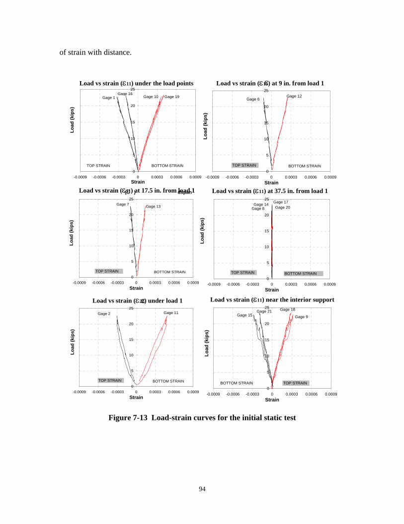
( ) p Load Vs Strain ( 11) at 9 in. from midspan
Load Vs Strain 11 at 17.5 in. from mi ( ) p
Load Vs Strain in the negative moment regionLoad Vs Strain ( 22) at Midspan
of strain with distance.
εLoad vs strain (ε11) under the load points Load vs strain (ε11) at 9 in. from load 1
0
5
10
15
20
25
Load
(kip
s)
GagGage 10
0
5
10
15
20
25
Load
(kip
s)
Gage 1 e 16
Gage 19
BOTTOM STRAIN TOP STRAIN
Gage 12 Gage 6
BOTTOM STRAIN TOP STRAIN
-0.0009 -0.0006 -0.0003 0 0.0003 0.0006 0.0009 -0.0009 -0.0006 -0.0003 0 0.0003 0.0006 0.0009 Strain Strain
(ε dspanLoad vs strain (ε11) ) at 17.5 in. from load 1 Load vs strain (ε11) at 37.5 in. from load 1
0
5
10
15
20
25
Load
(kip
s)
0
5
10
15
20
25 )
Gage 7 Gage 13
BOTTOM STRAIN TOP STRAIN
Load
(kip
sGage 8 Gage 14
Gage 20 Gage 17
BOTTOM STRAIN TOP STRAIN
-0.0009 -0.0006 -0.0003 0 0.0003 0.0006 0.0009 -0.0009 -0.0006 -0.0003 0 0.0003 0.0006 0.0009 Strain Strain
Load vs strain (ε22ε) under load 1 Load vs strain (ε11) near the interior support
0
5
10
15
20
25
Load
(kip
s)
0
5
10
15
20
25
Load
(kip
s)
Gage 15 Gage 21
Gage 9
Gage 18
BOTTOM STRAIN TOP STRAIN
Gage 2 Gage 11
BOTTOM STRAIN TOP STRAIN
-0.0009 -0.0006 -0.0003 0 0.0003 0.0006 0.0009 -0.0009 -0.0006 -0.0003 0 0.0003 0.0006 0.0009 Strain Strain
Figure 7-13 Load-strain curves for the initial static test
94
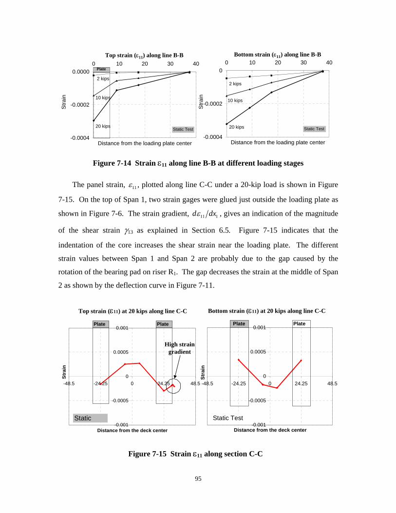
Top Strain (ε11) along line B-B Bottom Strain (ε11) along line B-B0
Top strain (ε11) along line B-B Bottom strain (ε11) along line B-B 10 20 30 40 0 10 20 30 40
in
2 kips
ips
ips
0
2 ki
ips
-0.0004
-0.0002
0.0000 S
tra
10 k
20 kStatic Test
Plate
-0.0004
-0.0002 Stra
in
ps
10 k
20 kips Static Test
Distance from the loading plate center Distance from the loading plate center
Figure 7-14 Strain ε11 along line B-B at different loading stages
The panel strain, ε , plotted along line C-C under a 20-kip load is shown in Figure 11
7-15. On the top of Span 1, two strain gages were glued just outside the loading plate as
shown in Figure 7-6. The strain gradient, dε dx 1 , gives an indication of the magnitude 11
of the shear strain γ13 as explained in Section 6.5. Figure 7-15 indicates that the
indentation of the core increases the shear strain near the loading plate. The different
strain values between Span 1 and Span 2 are probably due to the gap caused by the
rotation of the bearing pad on riser R1. The gap decreases the strain at the middle of Span
2 as shown by the deflection curve in Figure 7-11.
Top strain (ε11) at 20 kips along line C-C Bottom strain (ε11) at 20 kips along line C-C
0 0
0 0
Plate
-0.001
-0.0005
0.0005
0.001
-48.5 -24.25 24.25 48.5
Stra
in
Plate
Static
Plate
High strain gradient
-0.001
-0.0005
0.0005
0.001
-48.5 -24.25 24.25 48.5
Stra
in
Static Test
Plate
Distance from the deck center Distance from the deck center
Figure 7-15 Strain ε11 along section C-C
95
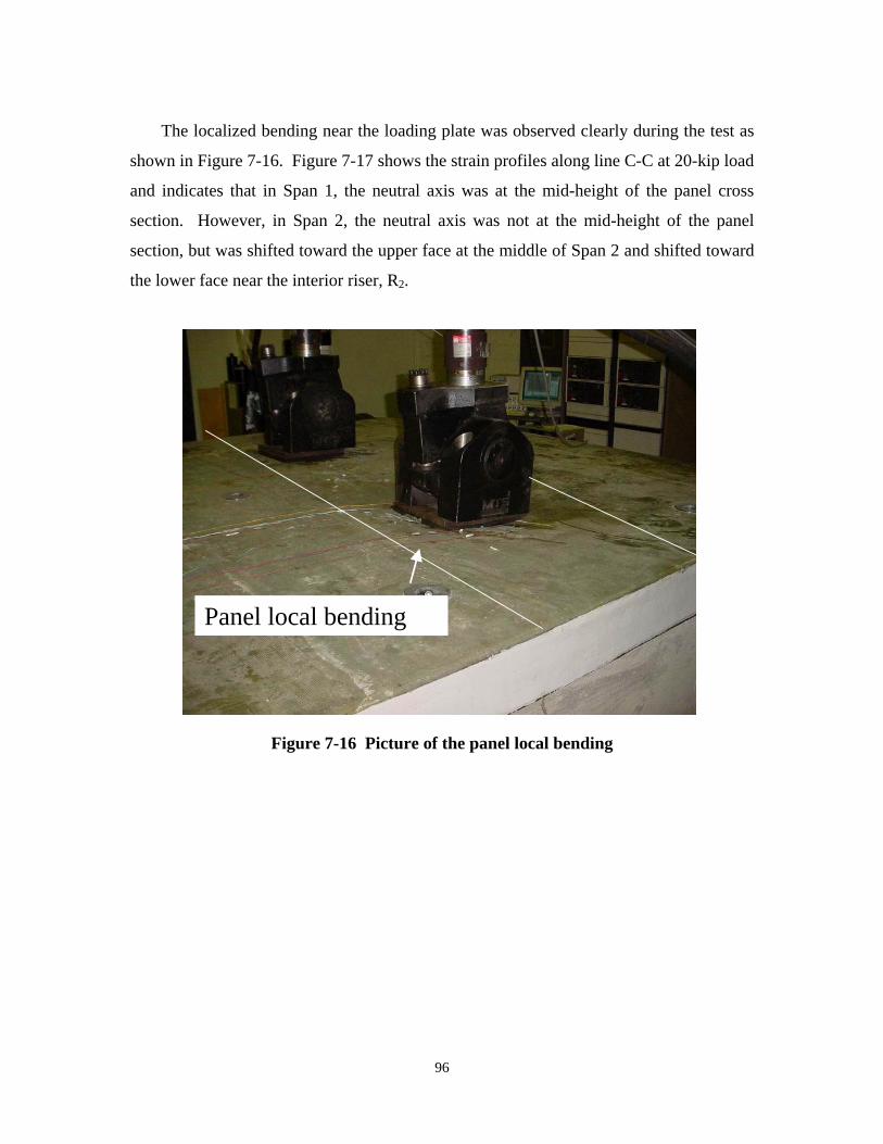
The localized bending near the loading plate was observed clearly during the test as
shown in Figure 7-16. Figure 7-17 shows the strain profiles along line C-C at 20-kip load
and indicates that in Span 1, the neutral axis was at the mid-height of the panel cross
section. However, in Span 2, the neutral axis was not at the mid-height of the panel
section, but was shifted toward the upper face at the middle of Span 2 and shifted toward
the lower face near the interior riser, R2.
Panel local bending
Figure 7-16 Picture of the panel local bending
96
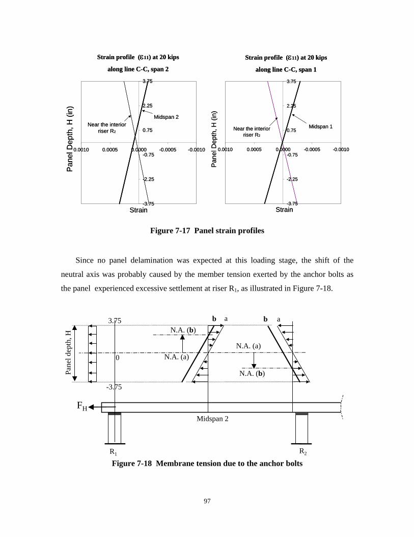
Strain profile (ε11) at 20 kipsStrain profile (ε11) at 20 kips Strain profile (ε11) at 20 kipsStrain profile (ε11) at 20 kips
along line C-C, span 2along line C-C, span 2 along line C-C, span 1along line C-C, span 1
-3.75
-2.25
-0.75
0.75
2.25
3.75
-0.0010-0.00050.00000.00050.0010
Pan
el D
epth
, H (i
n)
Midspan 2 Near the interior
riser R2
-3.75
-2.25
-0.75
0.75
2.25
3.75
-0.0010-0.00050.00000.00050.0010
Pan
el D
epth
, H (i
n)
Midspan 2Near the interior
riser R2
-3.75
-2.25
-0.75
0.75
2.25
3.75
-0.0010-0.00050.00000.00050.0010
Pan
el D
epth
, H (i
n)
Midspan 1Near the interior riser R2
-3.75
-2.25
-0.75
0.75
2.25
3.75
-0.0010-0.00050.00000.00050.0010
Pan
el D
epth
, H (i
n)
Midspan 1Near the interior riser R2
StrainStrain StrainStrain
Figure 7-17 Panel strain profiles
Since no panel delamination was expected at this loading stage, the shift of the
neutral axis was probably caused by the member tension exerted by the anchor bolts as
the panel experienced excessive settlement at riser R1, as illustrated in Figure 7-18.
FH
-3.75
3.75
Pane
l dep
th, H
a
0
N.A. (b) b
N.A. (a)
ab
N.A. (b)
N.A. (a)
Midspan 2
R1 R2
Figure 7-18 Membrane tension due to the anchor bolts
97

It must be mentioned that if the neutral axis shifts in opposite directions at
midspan and near the interior riser, the cause is most likely the horizontal force.
Conversely, if the neutral axis shifts in same direction, the cause could be the
delamination of one of the two faces.
7.6 Fatigue Test
The aim of the fatigue test was to investigate the influence of the load cycles on
the load carrying capacity of the panel and on the performance of the anchor bolts. The
fatigue test had three different loading phases as described in detail in Section 7.4. In
Phase 1 (from 0 to 15,200 cycles), the loads in Actuators 1 and 2 were 180° off-phase
with a peak load of 40 kips. In Phase 2 (from 15,200 to 370,200 cycles), only Actuator 1
was used with a peak load of 22 kips. In Phase 3 (from 370,200 to 1,500,000 cycles),
only Actuator 1 was used with a peak load of 31 kips.
7.6.1 Phase 1 - 0 to 15,200 cycles
The two spans were loaded by two actuators with sine waves that were 180° off-
phase and a maximum load of 40 kips in each actuator. At about 14,000 cycles, Span 2
started emitting a strong noise near the loading plate. Inspection of the panel did not
show any external damage. The noise was very likely caused by the delamination of the
upper face from the core. Between 15,000 and 15,200 cycles, data were recorded for 200
cycles (Cyclic data 1 in Table 7-2). The load-strain curves are shown in Figure 7-19.
98
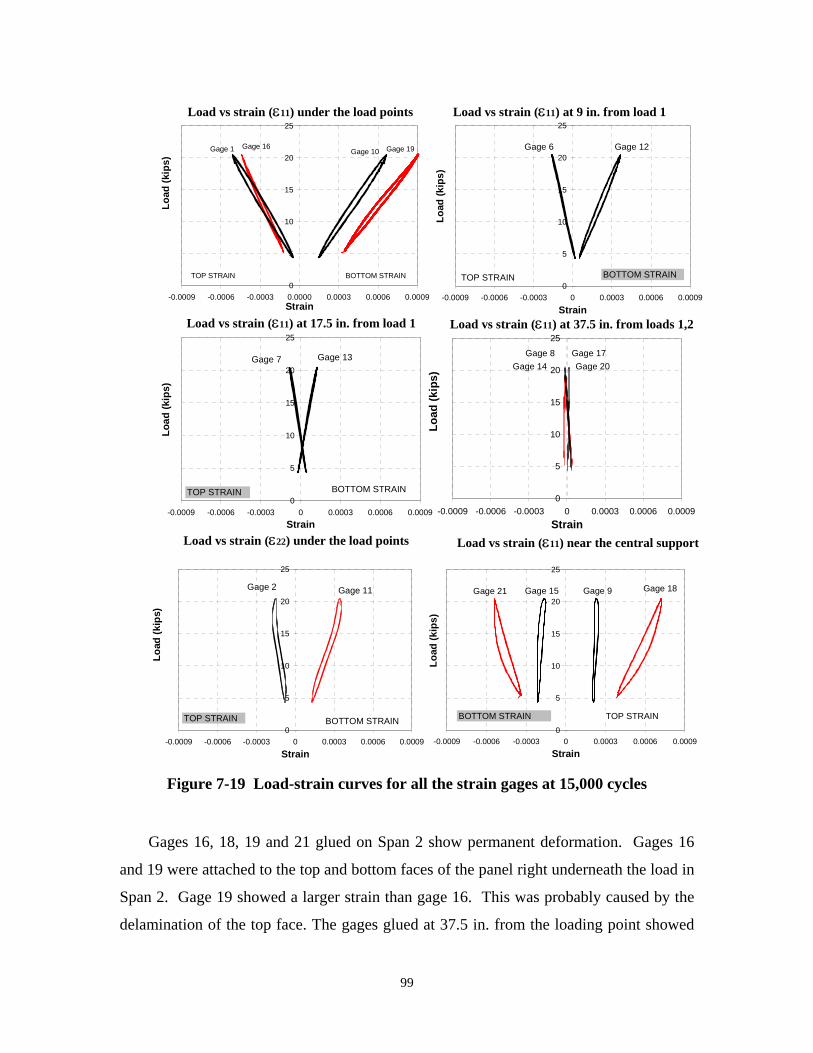
Load vs strain (ε11) under the load points Load vs strain (ε11) at 9 in. from load 1
0
5
10
15
20
25
16
0
5
10
15
20
25
()
Load
(kip
s) Gage 1 Gage
Gage 10 Gage 19
BOTTOM STRAIN TOP STRAIN
Load
kips
Gage 12 Gage 6
BOTTOM STRAIN TOP STRAIN
-0.0009 -0.0006 -0.0003 0.0000 0.0003 0.0006 0.0009 -0.0009 -0.0006 -0.0003 0 0.0003 0.0006 0.0009 Strain Strain
Load vs strain (ε11) at 17.5 in. from load 1 Load vs strain (ε11) at 37.5 in. from loads 1,2
0
5
10
15
20
25
(
13
0
5
10
15
20
25
Load
kips
)
GageGage 7
BOTTOM STRAIN TOP STRAIN
Load
(kip
s)
Gage 8 Gage 14 Gage 20
Gage 17
-0.0009 -0.0006 -0.0003 0 0.0003 0.0006 0.0009 -0.0009 -0.0006 -0.0003 0 0.0003 0.0006 0.0009 Strain Strain
Load vs strain (ε22) under the load points Load vs strain (ε11) near the central support
0
5
10
15
20
25
(ki
0
5
10
15
20
25
9
Load
ps)
Gage 2 Gage 11
BOTTOM STRAIN TOP STRAIN
Load
(kip
s)
Gage 15 Gage 21 Gage Gage 18
BOTTOM STRAIN TOP STRAIN
-0.0009 -0.0006 -0.0003 0 0.0003 0.0006 0.0009 -0.0009 -0.0006 -0.0003 0 0.0003 0.0006 0.0009
Strain Strain
Figure 7-19 Load-strain curves for all the strain gages at 15,000 cycles
Gages 16, 18, 19 and 21 glued on Span 2 show permanent deformation. Gages 16
and 19 were attached to the top and bottom faces of the panel right underneath the load in
Span 2. Gage 19 showed a larger strain than gage 16. This was probably caused by the
delamination of the top face. The gages glued at 37.5 in. from the loading point showed
99
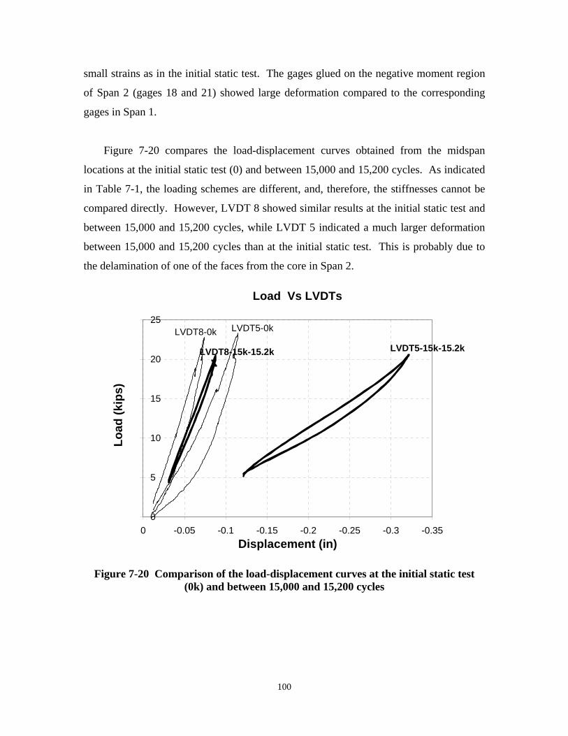
small strains as in the initial static test. The gages glued on the negative moment region
of Span 2 (gages 18 and 21) showed large deformation compared to the corresponding
gages in Span 1.
Figure 7-20 compares the load-displacement curves obtained from the midspan
locations at the initial static test (0) and between 15,000 and 15,200 cycles. As indicated
in Table 7-1, the loading schemes are different, and, therefore, the stiffnesses cannot be
compared directly. However, LVDT 8 showed similar results at the initial static test and
between 15,000 and 15,200 cycles, while LVDT 5 indicated a much larger deformation
between 15,000 and 15,200 cycles than at the initial static test. This is probably due to
the delamination of one of the faces from the core in Span 2.
Load Vs LVDTs
0
5
10
15
20
25
LVDT8-15k-15.2k
LVDT8-0k LVDT5-0k
Load
(kip
s)
LVDT5-15k-15.2k
0 -0.05 -0.1 -0.15 -0.2 -0.25 -0.3 -0.35 Displacement (in)
Figure 7-20 Comparison of the load-displacement curves at the initial static test (0k) and between 15,000 and 15,200 cycles
100
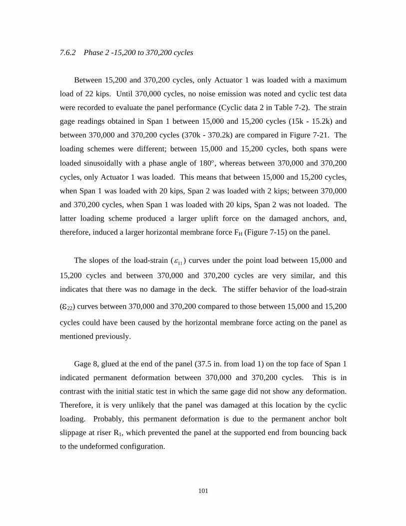
7.6.2 Phase 2 -15,200 to 370,200 cycles
Between 15,200 and 370,200 cycles, only Actuator 1 was loaded with a maximum
load of 22 kips. Until 370,000 cycles, no noise emission was noted and cyclic test data
were recorded to evaluate the panel performance (Cyclic data 2 in Table 7-2). The strain
gage readings obtained in Span 1 between 15,000 and 15,200 cycles (15k - 15.2k) and
between 370,000 and 370,200 cycles (370k - 370.2k) are compared in Figure 7-21. The
loading schemes were different; between 15,000 and 15,200 cycles, both spans were
loaded sinusoidally with a phase angle of 180°, whereas between 370,000 and 370,200
cycles, only Actuator 1 was loaded. This means that between 15,000 and 15,200 cycles,
when Span 1 was loaded with 20 kips, Span 2 was loaded with 2 kips; between 370,000
and 370,200 cycles, when Span 1 was loaded with 20 kips, Span 2 was not loaded. The
latter loading scheme produced a larger uplift force on the damaged anchors, and,
therefore, induced a larger horizontal membrane force FH (Figure 7-15) on the panel.
The slopes of the load-strain ( ε ) curves under the point load between 15,000 and11
15,200 cycles and between 370,000 and 370,200 cycles are very similar, and this
indicates that there was no damage in the deck. The stiffer behavior of the load-strain
(ε22) curves between 370,000 and 370,200 compared to those between 15,000 and 15,200
cycles could have been caused by the horizontal membrane force acting on the panel as
mentioned previously.
Gage 8, glued at the end of the panel (37.5 in. from load 1) on the top face of Span 1
indicated permanent deformation between 370,000 and 370,200 cycles. This is in
contrast with the initial static test in which the same gage did not show any deformation.
Therefore, it is very unlikely that the panel was damaged at this location by the cyclic
loading. Probably, this permanent deformation is due to the permanent anchor bolt
slippage at riser R1, which prevented the panel at the supported end from bouncing back
to the undeformed configuration.
101
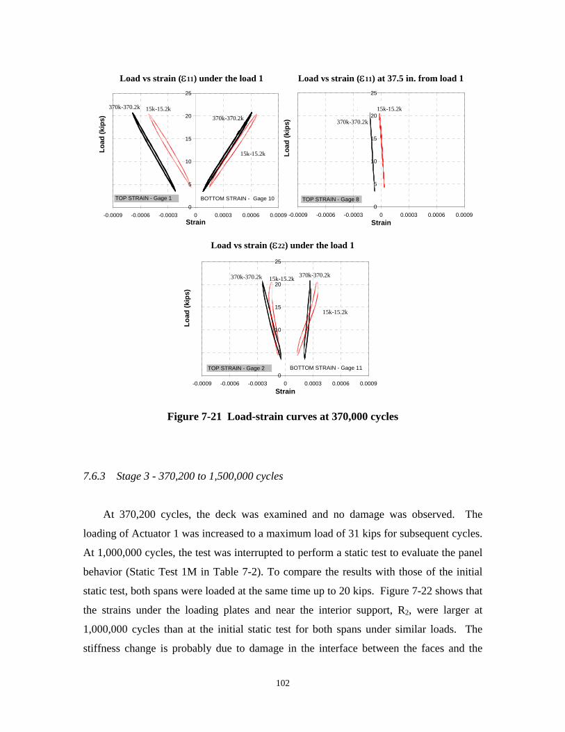
Load Vs Strain (ε11) at 37.5 in from midspan 1
70k k
Load Vs Strain (ε11) at Midspan 1
370k 15k 370k 5k
Load Vs Strain (ε22) at Midspan
370k 15k 370k k
Load vs strain (ε11) under the load 1 Load vs strain (ε11) at 37.5 in. from load 1
0
5
10
15
20
25
Load
(kip
s)
TOP STRAIN - Gage 8
3 15
0
5
10
15
20
25 Lo
ad (k
ips)
BOTTOM STRAIN Gage 10TOP STRAIN - Gage 1
1370k-370.2k
370k-370.2k
15k-15.2k
15k-15.2k
370k-370.2k
15k-15.2k
-0.0009 -0.0006 -0.0003 0 0.0003 0.0006 -0.00090.0009 -0.0006 -0.0003 0 0.0003 0.0006 0.0009 Strain Strain
Load vs strain (ε22) under the load 1
0
5
10
15
20
25
Load
(kip
s)
BOTTOM STRAIN - Gage 11TOP STRAIN - Gage 2
15370k-370.2k 15k-15.2k 370k-370.2k
15k-15.2k
-0.0009 -0.0006 -0.0003 0 0.0003 0.0006 0.0009 Strain
Figure 7-21 Load-strain curves at 370,000 cycles
7.6.3 Stage 3 - 370,200 to 1,500,000 cycles
At 370,200 cycles, the deck was examined and no damage was observed. The
loading of Actuator 1 was increased to a maximum load of 31 kips for subsequent cycles.
At 1,000,000 cycles, the test was interrupted to perform a static test to evaluate the panel
behavior (Static Test 1M in Table 7-2). To compare the results with those of the initial
static test, both spans were loaded at the same time up to 20 kips. Figure 7-22 shows that
the strains under the loading plates and near the interior support, R2, were larger at
1,000,000 cycles than at the initial static test for both spans under similar loads. The
stiffness change is probably due to damage in the interface between the faces and the
102
103
core. In particular, in Span 2, the strain near the middle support (negative moment
region) at 1,000,000 cycles is more than four times larger than the strain at 0 cycle.
Load Vs Strain in the negative moment region
0
5
10
15
20
25
-0.0009 -0.0006 -0.0003 0 0.0003 0.0006 0.0009Strain
Load
(kip
s)
BOTTOM STRAIN - Gage 21 TOP STRAIN - Gage 18
1M0k
1M0k
Load Vs Strain (ε11) at Midspan 1
0
5
10
15
20
25
-0.0009 -0.0006 -0.0003 0 0.0003 0.0006 0.0009Strain
Load
(kip
s)
BOTTOM STRAIN - Gage TOP STRAIN - Gage 1
1M 1M0k 0k
Load Vs Strain (ε11) at Midspan (2)
0
5
10
15
20
25
-0.0009 -0.0006 -0.0003 0 0.0003 0.0006 0.0009Strain
Load
(kip
s)
BOTTOM STRAIN - Gage 19TOP STRAIN - Gage 16
0k 0k1M 1M
Load Vs Strain in the negative moment region
0
5
10
15
20
25
-0.0009 -0.0006 -0.0003 0 0.0003 0.0006 0.0009Strain
Load
(kip
s)
BOTTOM STRAIN - Gage 15 TOP STRAIN - Gage 9
1M0k
1M
0k
Load vs strain (ε11) under load 2 Load vs strain (ε11) under load 1
Load vs strain (ε11) near the interior support Load vs strain (ε11) near the interior support
Span 2 Span 1
Figure 7-22 Load-strain curves at 1,000,000 cycles
The strain profiles in Figure 7-23 indicate that the neutral axis in Span 1 did not
change position during the fatigue loading. The softening was probably caused by the
delamination of Span 2. For Span 2, near the interior riser, R2, the neutral axis at
1,000,000 cycles shifted upward, whereas at midspan, the neutral axis did not move, as
shown in Figure 7-24. The progressive damage of the panel is different from that of the
beams tested previously. In the beam tests, when one of the two faces delaminated, the
neutral axis shifted from its initial position (the neutral axis shifted upward if the lower
face debonded and downward if the upper face debonded) and the failure ensued. In the
panel test, the delamination of the faces was not necessarily followed by collapse because
damage could be local and stress redistribution could occur.
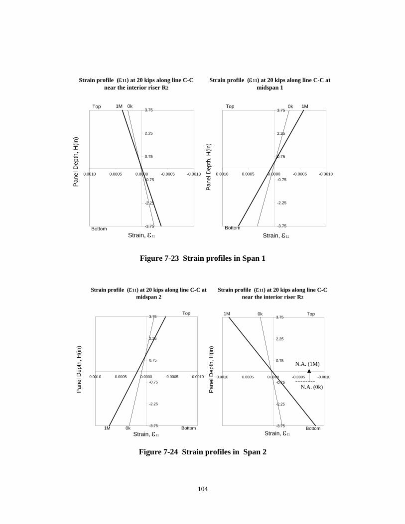
Strain profile (ε11) at 20 kips along line C-C Strain profile (ε11) at 20 kips along line C-C at near the interior riser R2 midspan 1
1M 0k 0k 1M
Pan
el D
epth
, H(in
)
Top Top 3.75
Bottom Bottom
Strain, ε11 Strain, ε11
0.75
2.25
3.75
0.00000.0005
Pane
l Dep
th, H
(in)
0.75
2.25
-0.00050.0000
-3.75
-2.25
-0.75 -0.0010 -0.0005 0.0010
-3.75
-2.25
-0.75 -0.0010 0.0005 0.0010
Figure 7-23 Strain profiles in Span 1
(ε11) at 20 kips along line C-C at Strain profile (ε11Strain profile ) at 20 kips along line C-C midspan 2 near the interior riser R2
, ε11
Pan
el D
epth
, H(in
)
1M 0k
Strain, ε11
(in)
1M
N.A. (1M)
-3.75
-2.25
-0.75
0.75
2.25
3.75
-0.0010 -0.0005 0.0000 0.0005 0.0010
Strain
Top
Bottom
N.A. (0k)
-3.75
-2.25
-0.75
0.75
2.25
3.75
-0.0010 -0.0005 0.0000 0.0005 0.0010
Pan
el D
epth
, H
0k
Top
Bottom
Figure 7-24 Strain profiles in Span 2
104

Figure 7-24 indicates that, near the interior riser, the top face was carrying less load
than the bottom face at the initial static test and that the two faces were carrying the same
amount of load at 1,000,000 cycles. This indicates that the bottom face could have
delaminated after the fatigue load cycles.
At 1,500,000 cycles, Span 1 started emitting a strong noise. Then, a static test
was performed to evaluate the panel behavior (Static Test 1.5M in Table 7-2). Figure
7-25(a) compares the static load-actuator displacement responses at 1,000,000 and
1,500,000 cycles. The figure does not represent the true flexibility of the panel because
the actual displacement includes the flexibility of the steel reaction frame that supported
the actuator as well as the support settlements at the risers. The graph is used only to
show that the overall stiffness decreased with load cycles. Figure 7-25(b) shows the
comparison of the adjusted displacement at the middle of Span 1 at 1,500,000 cycles
(1.5M) and the LVDT 8 reading at the initial static test (0k). To find the adjusted
midspan displacement, the stiffness of the steel frame is first evaluated by using the
initial static test data. Then, using this stiffness the steel frame displacement is calculated
and subtracted from the actuator displacement to find the adjusted midspan displacement
at 1,500,000 cycles. As shown, the stiffness of Span 1 decreased with increasing loading
cycles probably because of the local delamination of the upper face from the core.
Figure 7-26 shows the load-strain curves at 0, 1,000,000 and 1,500,000 cycles.
The strain profiles for Span 1 in Figure 7-27 indicate that the neutral axis moved upward
from 0 to 1,500,000 cycles indicating that the lower face delaminated from the core.
105
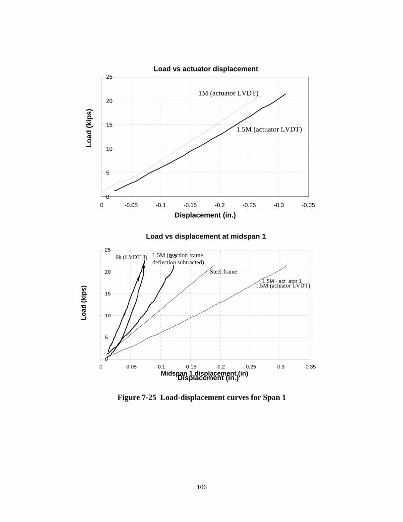
Load vs midspan 1 displacement
u
0k M steel frame
Load vs actuator 1
Displacement (in)
1.5M - actuator 1
1M - actuator 1
Load vs actuator displacement
Load
(kip
s)
Load
(kip
s)
0
5
10
15
20
25
)
)
1M (actuator LVDT
1.5M (actuator LVDT
0 -0.05 -0.1 -0.15 -0.2 -0.25 -0.3 -0.35
Displacement (in.)
Load vs displacement at midspan 1
0
5
10
15
20
25
```
1.5( ()
) 1.5M - act ator 1
0k LVDT 8) 1.5M reaction frame deflection subtracted
Steel frame
1.5M (actuator LVDT
0 -0.05 -0.1 -0.15 -0.2 -0.25 -0.3 -0.35 Midspan 1 displacement (in) Displacement (in.)
Figure 7-25 Load-displacement curves for Span 1
106
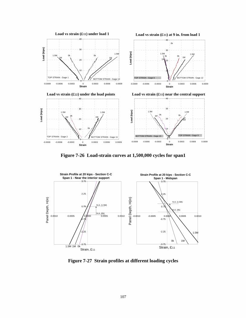
Load Vs Strain (ε11) at Midspan Load Vs Strain (ε11) at 9 in. from midspan
Load Vs Strain in the negative moment regionLoad Vs Strain (ε22) at Midspan
Load vs strain (ε11) under load 1 Load vs strain (ε11) at 9 in. from load 1
0
10
20
30
40
()
0k 0k 1M 1M
0
10
20
30
40
)
1M
0k
0k 1M
0k
Load
kips
BOTTOM STRAIN - Gage 10 TOP STRAIN - Gage 1
1.5M 1.5M
Load
(kip
s
BOTTOM STRAIN - Gage 12 TOP STRAIN - Gage 6
1.5M 1.5M
-0.0009 -0.0006 -0.0003 0 0.0003 0.0006 0.0009 -0.0009 -0.0006 -0.0003 0 0.0003 0.0006 0.0009 Strain Strain
Load vs strain (ε22) under the load points Load vs strain (ε11) near the central support
0
10
20
30
40
)
1M 0k
1M
0k
0
10
20
30
40
1M 0k
0k
1M
Load
(kip
s
BOTTOM STRAIN - Gage 15 TOP STRAIN - Gage 9
1.5M 1.5M
Load
(kip
s)
BOTTOM STRAIN - Gage 11 TOP STRAIN - Gage 2
1.5M 1.5M
-0.0009 -0.0006 -0.0003 0 0.0003 0.0006 0.0009 -0.0009 -0.0006 -0.0003 0 0.0003 0.0006 0.0009
Strain Strain
Figure 7-26 Load-strain curves at 1,500,000 cycles for span1
Strain Profile at 20 kips - Section C-C Strain Profile at 20 kips - Section C-C Span 1 - Near the interior support Span 1 - Midspan
Pan
el D
epth
, H(in
)
1M0k
1.5M
(
Pan
el D
epth
, H(in
)
)
( )
-3.75
-2.25
-0.75
0.75
2.25
3.75
-0.0010 -0.0005 0.0000 0.0005 0.0010
N.A. 1.5M)
N.A. (0k)
-3.75
-2.25
-0.75
0.75
2.25
3.75
-0.0010 -0.0005 0.0000 0.0005 0.0010
N.A. (1.5M
N.A. 0k
1.5M 1M 0kStrain, ε11
Strain, ε11
Figure 7-27 Strain profiles at different loading cycles
107

7.7 Final Static Test
After the fatigue test was completed, the two spans were loaded one at a time up to Lo
ad (k
ips)
100 kips. Figure 7-28 shows the load-actuator displacement response for Span 1. The
beams that were tested previously and the panel behaved differently after delamination.
For three out of the four beams tested, the failure was brittle. One beam showed a
ductile-like behavior because the upper face was not glued uniformly to the core and had
progressive delamination. The latter is similar to the panel behavior. In the panel, a
crack formed in the face-core interface near the loading plate when the maximum shear
stress exceeded the interface shear strength and the crack propagated gradually causing a
ductile-like failure.
.
Load vs actuator displacement, span 1 120
100
80
60
40
20
0 0 1 2 3 4
1
2 3
4
Displacement (in.)
Figure 7-28 Load- actuator displacement curve for Span 1
The strain profiles for Span 1 at different loading stages, 1, 2, 3 and 4 in Figure 7-28,
are shown in Figure 7-29 and Figure 7-30. Both strain profiles show that the neutral axis
moved downward between stages 1 and 2. This response indicates that the top face
delaminated from the core.
108

Figure 7-29 shows that the strain at the bottom face near the interior riser was zero at
stage 2, and the strain became positive at stage 3. Furthermore, at stage 3, the neutral
axis near the interior riser was outside of the cross section. This is possible only if there
was a horizontal tensile force acting on the panel (see Figure 7-18), which was probably
caused by the anchor bolts as explained earlier. Figure 7-30 indicates that between stages
2 and 3, the neutral axis at midspan moved upward confirming that there was a horizontal
force acting on the panel.
Strain profile (ε11) along line C-C near the interior riser 2
Pan
el D
epth
, H (i
n.)
1
3 4
)
) -3.75
-2.25
-0.75
0.75
2.25
3.75
-0.0020 -0.0010 0.0000 0.0010 0.0020
N.A. (1
N.A. (2
Strain, ε11
Figure 7-29 Strain profiles in Span 1 near the interior riser at 1,500,000 cycles
109
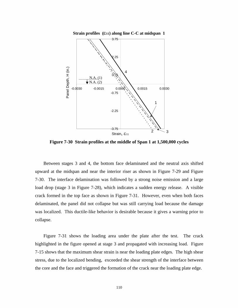
Strain profiles (ε11) along line C-C at midspan 1
-3.75
-2.25
-0.75
0.75
2.25
3.75
-0.0015 0.0015
Pan
el D
epth
, H (i
n.)
1
2
4 ))
-0.0030 0.0000 0.0030
N.A. (1N.A. (2
Strain, ε11 3
Figure 7-30 Strain profiles at the middle of Span 1 at 1,500,000 cycles
Between stages 3 and 4, the bottom face delaminated and the neutral axis shifted
upward at the midspan and near the interior riser as shown in Figure 7-29 and Figure
7-30. The interface delamination was followed by a strong noise emission and a large
load drop (stage 3 in Figure 7-28), which indicates a sudden energy release. A visible
crack formed in the top face as shown in Figure 7-31. However, even when both faces
delaminated, the panel did not collapse but was still carrying load because the damage
was localized. This ductile-like behavior is desirable because it gives a warning prior to
collapse.
Figure 7-31 shows the loading area under the plate after the test. The crack
highlighted in the figure opened at stage 3 and propagated with increasing load. Figure
7-15 shows that the maximum shear strain is near the loading plate edges. The high shear
stress, due to the localized bending, exceeded the shear strength of the interface between
the core and the face and triggered the formation of the crack near the loading plate edge.
110
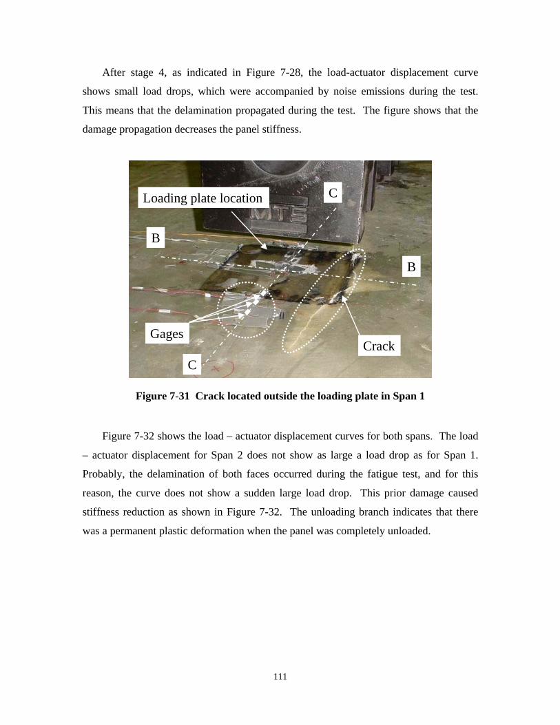
After stage 4, as indicated in Figure 7-28, the load-actuator displacement curve
shows small load drops, which were accompanied by noise emissions during the test.
This means that the delamination propagated during the test. The figure shows that the
damage propagation decreases the panel stiffness.
Crack
Loading plate location
Gages
C
C
B
B
Figure 7-31 Crack located outside the loading plate in Span 1
Figure 7-32 shows the load – actuator displacement curves for both spans. The load
– actuator displacement for Span 2 does not show as large a load drop as for Span 1.
Probably, the delamination of both faces occurred during the fatigue test, and for this
reason, the curve does not show a sudden large load drop. This prior damage caused
stiffness reduction as shown in Figure 7-32. The unloading branch indicates that there
was a permanent plastic deformation when the panel was completely unloaded.
111

Load vs actuator displacements Lo
ad (k
ips)
120
100
80
60
40
20
0 0 1 2 3
Span 1
Span 2
Displacement (in.)
Figure 7-32 Load – actuator displacements for Span 1 and 2
7.8 Final Remarks
The initial static test has indicated that the mechanical anchor that attached the GFRP
panel to the concrete supports did not work very well. Some of the anchor bolts on an
external support slipped when each of the two spans was subjected to a load up to 22
kips. Because of this observation, the anchor bolts have been switched to epoxy anchor
for the O’Fallon Park bridge.
112
8 ANALYSIS OF PANEL BEHAVIOR USING PLATE THEORY
8.1 Introduction
The Kirchhoff-Love plate theory is used here to analyze a GFRP panel that has the
same cross-sectional properties as the O’Fallon Park deck to gain a better insight of the
experimental results. The major drawback of this theory is that it does not take into
account the shear deformation. Consequentially, the Kirchhoff-Love theory gives
accurate results only if the ratio of the smaller lateral dimension of the plate to its
thickness is at least ten (Szilard 1974). In the case of the O’Fallon Park deck, this ratio is
only 6.5. Hence, to check the accuracy of the analytical solution, the panel is analyzed in
Chapter 9 with the finite element method.
In the actual test, the panel had two spans. However, in the analytical solution, the
panel is assumed to be simply supported along two opposite edges and free along the
other two for sake of simplicity. The panel model has a span of 48.5 in. (center-to-center
distance of the risers in the original test panel) and a variable width, b, as shown in Figure
8-1.
113
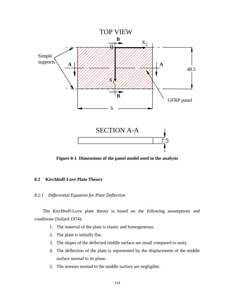
EQUATION CHAPTER 8 SECTION 1
TOP VIEW
GFRP panel
AAsupports
B
B x2
x1
0
b
48.5
SECTION A-A
Simple
Figure 8-1 Dimensions of the panel model used in the analysis
8.2 Kirchhoff-Love Plate Theory
8.2.1 Differential Equation for Plate Deflection
The Kirchhoff-Love plate theory is based on the following assumptions and
conditions (Szilard 1974):
1. The material of the plate is elastic and homogeneous.
2. The plate is initially flat.
3. The slopes of the deflected middle surface are small compared to unity.
4. The deflection of the plate is represented by the displacement of the middle
surface normal to its plane.
5. The stresses normal to the middle surface are negligible.
114
6. The deflection is small compared to the plate thickness. The maximum
deflection is less than one fiftieth of the smaller span length.
7. The thickness of the plate is small compared to the other dimensions. The
smaller lateral dimension of the plate is at least ten times larger than its
thickness.
8. During loading, plane sections remain plane; the deformation due to
transverse shear is neglected.
The first six assumptions are valid for the panel studied here. However, the ratio
of the smaller lateral dimension to the thickness is only 6.5, and, hence, condition 7 does
not apply here. As a consequence, the shear deformation cannot be neglected, and,
therefore, assumption 8 is not valid. In spite of this, the Kirchhoff-Love plate theory is
used here for the sake of simplicity and with an intention of checking its accuracy for the
thick panel considered here using a finite element model. It can be used to develop a
better understanding of the behavior of the panel and the influence of the orthotropy
introduced by the honeycomb construction.
To set up the orthotropic plate equation based on the Kirchhoff-Love theory, it is
necessary to follow these steps:
1. Consider the equilibrium of the external and internal forces acting on the plate.
2. Use an orthotropic elastic material law to link strains to stresses.
3. Express the strains and stresses as functions of the displacement.
4. Express the internal forces as functions of the displacement.
1. Equilibrium
By using the Cartesian coordinate system shown in Figure 8-2 and assuming that
the plate is subjected only to lateral forces, it is possible to write the following
equilibrium equations:
∑ M = 0 ∑ M = 0 ∑ Fx 3 = 0(8.1)
x1 x 2
115
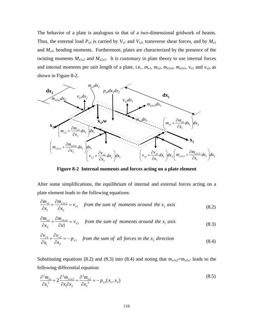
The behavior of a plate is analogous to that of a two-dimensional gridwork of beams.
Thus, the external load Px3 is carried by Vx1 and Vx2, transverse shear forces, and by Mx1
and Mx2, bending moments. Furthermore, plates are characterized by the presence of the
twisting moments Mx1x2 and Mx2x1. It is customary in plate theory to use internal forces
and internal moments per unit length of a plate, i.e., mx1, mx2, mx1x2, mx2x1, vx1 and vx2, as
shown in Figure 8-2.
x3,w
x1
x2
m dx2 vx1dx2
mx1dx2
mx2dx1
m dx1
vx2dx1
1 1 1 2
1
x x
m m x
∂+ ∂
m ∂v ∂ ∂
2 1 2 1 2 1
2
x x x x
m m x
∂+ ∂
2 2 2 1
2
x x
m m x
∂+ ∂
dx1
dx2 px3dx1dx2
x1x2
x2x1
dx dx
dx dx
dx dx
+∂
1 2 x x
xx
1
1 dx 1 dx 2 m 1 2 + ∂x1
dx 1 dx 2x x vx 2 + vx 2 dx 2 dx 1 vx1
∂x2
Figure 8-2 Internal moments and forces acting on a plate element
After some simplifications, the equilibrium of internal and external forces acting on a
plate element leads to the following equations:
x∂mx1 +∂mx1 2 = vx1 from the sum of moments around the x 2 axis (8.2)∂x1 ∂x2
x∂mx 2 +∂mx1 2 = vx 2 from the sum of moments around the x 1 axis (8.3)∂x2 ∂x1
∂vx1 ∂vx 2 = − p∂x1
+∂x2
x from the sum of all forces in the x 3 direction (8.4)3
Substituting equations (8.2) and (8.3) into (8.4) and noting that mx1x2=mx2x1 leads to the
following differential equation: 2∂2mx1 + 2 ∂ mx1
(8.5)2 +
∂2mx 2 = − p ( x x )x
∂x12 ∂x ∂x2 ∂x2
2 x 3 1 , 2 1
116

2. Orthotropic stress-strain Law
In the case of plane stress, five elastic constants are necessary for the description of
the orthotropic stress-strain relations:
Eε =
σ11 −υ21 σ 22 (8.6)
11 11 E22
Eε22 =
σ 22 −υ12 σ11
22 E11
τ12= G
γ 1212
Inverting equation (8.6), we can express the stresses in term of strains:
(8.7)σ11 =
E11 (ε +υ ε )1−υ υ 11 21 22
12 21
σ11 = E22 (ε +υ ε )
1−υ υ 22 12 1112 21
τ12 = G12γ12
3. Relation between strains and displacement
By using the compatibility condition, it is possible to express the strains in terms of
the displacement:
∂2 w (8.8)ε = −x3 = x3κ11 x1∂x1
2
∂2 wε22 = −x3 = x3κ x 2∂x22
∂2 wγ 12 = −2x3 = 2x3χx x2∂ ∂1
where w is the displacement in the x3 direction as defined in Figure 8-2, the κ's are the
curvatures, and χ is the warping of the plate.
4. Internal force-displacement relations
By integrating the stress components along the plate thickness H, the bending and
twisting moments are given by:
117
H / 2 mx1 = ∫−H
σ x dx 3 (8.9)
11 3 2
σ x dx 3mx 2 = ∫−
H
H
/ 2
22 3 2
m 1 2 = mx 2 1 = ∫−
H
H
/ 2τ x dx 3x x x 12 3
2
Substituting equations (8.7) and (8.8) into (8.9), the moments can be expressed in terms
of displacement, w: 2 2
m ∂ w ∂ w (8.10)
x1 = −D11 ∂x1
2 +υ21 ∂x22
2 2
m ∂ w ∂ w
x 2 = −D22 +υ12 ∂x12
∂x22
∂2 w m 1 2 = −2Dtx x ∂ ∂x x21
where D11 and D22 are the flexural rigidities of an orthotropic plate, and 2Dt = (1-υ )D1212
represents the torsional rigidity. For a plate with a uniform thickness,
E H 3 (8.11) = 11D11 2 )12(1 −ν12
E H 3 (8.12) = 22D22 2 )12(1 −ν 21
H 3 (8.13)Dt = G12 12
Finally, the substitution of equation (8.10) into (8.5) yields the governing differential
equation for orthotropic plates:
∂4 w ∂4 w ∂4 w (8.14)D + 2B 4 = px3
( x1, x2 )11 ∂x14 ∂x1
2∂x22 + D22 ∂x2
where B is the effective torsional rigidity:
1B = 2
(υ21D11 +υ12 D22 + 4Dt ) (8.15)
An exact solution of the governing differential equation, equation (8.14), must satisfy the
plate boundary conditions. For rectangular plates subjected to lateral loads, the Levi’s
118
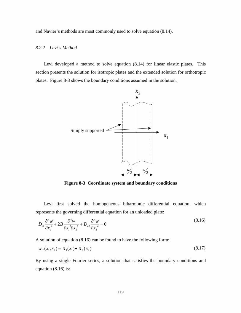
and Navier’s methods are most commonly used to solve equation (8.14).
8.2.2 Levi’s Method
Levi developed a method to solve equation (8.14) for linear elastic plates. This
section presents the solution for isotropic plates and the extended solution for orthotropic
plates. Figure 8-3 shows the boundary conditions assumed in the solution.
x2
Simply supported x1
2 a
2 a
Figure 8-3 Coordinate system and boundary conditions
Levi first solved the homogeneous biharmonic differential equation, which
represents the governing differential equation for an unloaded plate:
∂4 w ∂4 w ∂4 w (8.16)D + 2B 2 + D22 = 011 ∂x1
4 ∂x12∂x2 ∂x2
4
A solution of equation (8.16) can be found to have the following form:
w x1( , x ) = X1( x ) • X ( x ) (8.17)H 2 1 2 2
By using a single Fourier series, a solution that satisfies the boundary conditions and
equation (8.16) is:
119

∞ π (8.18)w x1( , x ) = ∑ X ( x )sin m x1
H 2 2m 2m=1 a
Substituting (8.18) into (8.16), we have
D 4 4 2 2 (8.19)
11 m π X 2m − 2B m π X II + D22 X IV = 04 2 2 m 2 ma a
X II X IVIn equation (8.19), and are the second derivative and fourth derivative of the
function X, respectively. The solution of equation (8.19) is of the form:
= Gerx2 (8.20)X 2m
where G is a constant and r are the four roots of the corresponding characteristic
equation:
B2
r mπ B D11 (8.21)
1,2,3,4 = ± ± D2 −
a D D 22 22 22
By defining (Timoshenko and Woinowsky-Krieger 1974)
B (8.22)µ =
D D2211
we obtain three different cases for the solution of equation (8.16):
1. Two double real roots if µ = 1, i.e., B = D D22 (8.23)
11
2. Four complex roots if µ < 1, i.e., B < D D22 11
3. Four real roots if µ > 1, i.e., B > D D22 11
It should be noticed that the first case represents an isotropic case.
In this study, to compare an isotropic plate with an orthotropic plate, both cases 1
and 2 are considered. The orthotropic solution uses the material properties given in Table
8-1. The values in Table 8-1 are obtained by modeling a 7.5-in. honeycomb sandwich
panel as a three layer laminate and using the classical lamination theory (Daniel and Ishai
1994) using the material properties shown in Table 3-2. The isotropic solution is based
120

12on the elastic modulus, E11, as well as the shear modulus, G12, and Poisson Ratio, υ ,
shown in Table 8-1.
Table 8-1 Equivalent stiffness properties of GFRP honeycomb sandwich panel
Elastic Moduli (ksi) Poisson Ratio E11 E22 G12 ν12 827 503 148 0.302
Substituting the values given in Table 8-1 in equations (8.11) and (8.12), we have µ
= 0.66. Thus, the solution for the orthotropic sandwich panel considered here is
represented by case 2.
Case1: Isotropic plates
In this case, D11=D22=D and µ =1. Hence, equation (8.19) can be simplified as: 2 2 4 4 (8.24)
X IV m π+ 2 m π X II + 4 X 2m = 0
2 m 2 2 ma a
The solution of equation (8.24) has the following form: π m x2
m x2 π π π
X 2m = A em x2 − m x2
+ D m x2 − m x2 (8.25)π π
e a aa + B + C e e a m m m ma a
Observing that the deflection and its derivatives approach zero at a large distance from
the x1 axis, we have Am=Bm=0. Therefore, the solution of equation (8.16) can be
represented by the following sine series: ∞ π π− m x2 π (8.26)
( ,w x x 2 ) = ∑(C + D m x2 )e a sin m x1 H 1 m m
m=1 a a
∂w Exploiting the condition of symmetry, i.e.,
dx2
x2 =0
= 0 , we have Cm=Dm. Therefore,
we can write equation (8.26) in the following form: ∞ π π− m x2 π (8.27)
( ,w x x 2 ) = ∑C (1 + m x2 )e a sin m x1
H 1 m m=1 a a
121
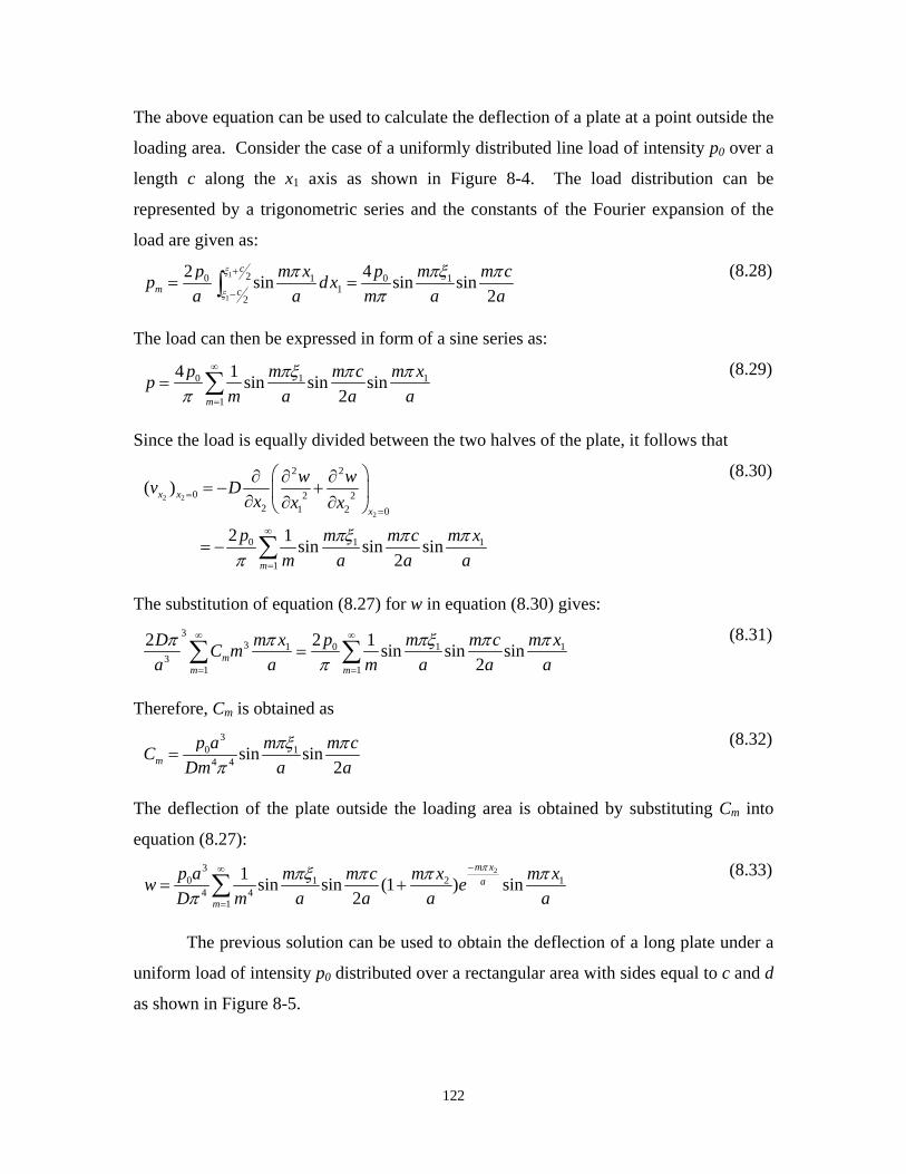
The above equation can be used to calculate the deflection of a plate at a point outside the
loading area. Consider the case of a uniformly distributed line load of intensity p0 over a
length c along the x1 axis as shown in Figure 8-4. The load distribution can be
represented by a trigonometric series and the constants of the Fourier expansion of the
load are given as: ξ1 +c
2 π 4 p0 sin mπξ1 sin m c (8.28)p =
2 p0 ∫ξ1 − sin m x1 dx1 =
π m a c
2 a mπ a 2a
The load can then be expressed in form of a sine series as: ∞ π π 14 p0 ∑ 1 sin mπξ1 sin m c sin m x (8.29)
p = π m=1 m a 2a a
Since the load is equally divided between the two halves of the plate, it follows that
2 (8.30)∂ ∂2 w ∂ w v( )x2 =0 = −D + 2 x2 ∂x2
∂x1
2 ∂x2 x2 =0
∞ π m x 1π0= −2 p ∑ 1 sin mπξ1 sin m c sin π m=1 m a 2a a
The substitution of equation (8.27) for w in equation (8.30) gives:
2Dπ 3
∑C m3 m x 1 = 2 p ∞ π m x 1
(8.31)∞ π 0 ∑ 1 sin mπξ1 sin m c sin π 3 ma m=1 a π m=1 m a 2a a
Therefore, Cm is obtained as 3 π (8.32)
0C = p a sin mπξ1 sin m c
m 4 4Dm π a 2a
The deflection of the plate outside the loading area is obtained by substituting Cm into
equation (8.27): −m x2p a3 ∞ 1 sin mπξ1 sin m c (1 + m x 2 π (8.33)
w = 04 ∑
π π )e a π
sin m x 1 4Dπ m=1 m a 2a a a
The previous solution can be used to obtain the deflection of a long plate under a
uniform load of intensity p0 distributed over a rectangular area with sides equal to c and d
as shown in Figure 8-5.
122
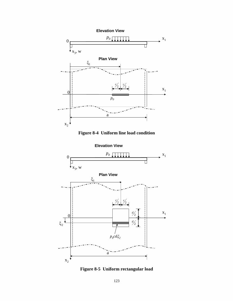
Elevation View p00 x1
x3, w
Plan View
x2
x1 2
c 2
c
0
ξ1
a
p0
Figure 8-4 Uniform line load condition
Elevation View
p00 x1
x3, w
Plan View
x2
x1
2 c
2c
2d
2d
0
ξ1
ξ2
a
p0cdξ2
Figure 8-5 Uniform rectangular load
123

To this end, consider a load of magnitude p0cdξ2 over an infinitesimal area (see Figure
8-5) at a distance ξ2 from the x1 axis. The infinitesimal load can be expressed in form of
a sine series as:
4 p ∞ mπξ1 sin mπ c mπ x1 (8.34)
p dξ = 0 dξ 2 ∑ 1 sin sin0 2 π m= 1 m a 2a a
The deflection produced by the infinitesimal load p0dξ2 at points outside the
loading area is obtained by substituting p0dξ2 for p0 and x2-ξ2 for x2 in equation (8.33).
The deflection produced by the entire load over the rectangular area is obtained by
integrating the resulting equation with respect to ξ 2 from - d2 to + d
p a
2 :
3 ∞ 1 sin mπξ mπ c mπ x1 (8.35)
w = 04 ∑ 1 sin sin ×4Dπ m= 1 m a 2a a
d − mπ (2 x2 − d ) − mπ (2 x2 + d ) 2a 2a d mπ
+ x2 − 2 e 2 a −
mπ
+ x2 + 2 e 2 a
The above equation is applicable to plate deflection outside the loading area.
Case 2: Orthotropic plates
The solution for an orthotropic plate can be found with a similar procedure used
for the isotropic case. By defining the following parameters (Timoshenko and
Woiwonowksi-Krieger 1974):
(8.36)
Dλ = 4
D22 α = aλ µ + µ 2 − 1 β =
aλ µ − µ 2 − 111 π π
the solution of equation (8.19) has the following form: mx2 mx2 − mx2 − mx2 (8.37)
β βX 2m = A e α + B e + C e α + D e m m m m
By observing that the deflection and its derivatives approach zero at a large distance from
the x1 axis, we have Am=Bm=0 and equation (8.37) can be simplified as − mx2 − mx2 (8.38)
βX 2m = C e α + D e m m
124

Equation (8.18) becomes: − mx2 − mx2 (8.39)∞ π w x x 2 ) = ∑ C e α + D e β sin m x1
H 1( , m m m a
∂ w From symmetry, it can be concluded that along the x1 axis,
dx2
x2 = 0
= 0 . Hence,
βD = − C and we can write equation (8.39) in the form: m mα
(8.40)∞ α β π w x x 2 ) = ∑ Cm e
− mx2
−β e
− mx2 sin m x1
H 1( , m α
a
Consider the case of a uniformly distributed line load of intensity p0 over a length c along
the x1 axis as shown in Figure 8-4. The load distribution can be represented by a
trigonometric series and the constants of the Fourier expansion of the load are given as: ξ1 + c 2 π 4 p0 sin mπξ1 sin m c (8.41)
p = 2 p0 ∫ξ1 −
sin m x1 dx 1 =π
m a c2 a mπ a 2a
The load can then be expressed in form of a sine series as: ∞ π π 14 p0 ∑
1 sin mπξ1 sin m c sin m x (8.42)p =
π m= 1 m a 2a a
Since the load is equally divided between the two halves of the plate, it follows that 2 (8.43)∂ ∂ 2 w ∂ w
v( )x2 = 0 = −∂ x2
D22 ∂ x22 + B 2 x2
∂ x1 x2 = 0
0 ∑ π π 1
π= −
2 p ∞ 1 sin mπξ1 sin m c sin m x
m= 1 m a 2a a
The constant Cm can be found by substituting equation (8.40) into (8.43)
α p a4 (8.44)0C = m 4 3 2 22π m D11 (α − β )
Therefore, equation (8.40) becomes
∞ 4 β π0( ,w x x 2 ) = ∑
α p a 2 2
− mx2 β − mx2 (8.45) H 1 4 3 am 2π m D11 (α − β ) e α −
α e sin m x 1
125

The above equation can be extended to find the deflection of a plate due to a load
uniformly distributed over a rectangular area as shown in Figure 8-5. The deflection
produced by the infinitesimal load p0dξ2 at points outside the loading area is obtained by
substituting p0dξ2 for p0 and x2-ξ2 for x2 in equation (8.45). The deflection produced by
the entire load over the rectangular area is obtained by integrating the resulting equation
with respect to ξ2 from - d2 to + d
2 :
2
w = p0a ∞ 1 sin mπξ mπ c (8.46)
1 sin ×3 ∑ 4 a 2aπ D D22 m=1 m11
e β0 sin mπ x1α sin mx2 + β0 cos mx2
−mx1 0
a α0 β0 where α0 and β0 are defined as:
(8.47)aλ 2 aλ 2α0 = β0 = π 1 − µ π 1 + µ
The above equation is applicable to plate deflection outside the loading area.
8.2.3 Navier’s Solution
Navier obtained the solution for the governing differential equation, equation (8.14),
for a plate with four simply supported edges and subjected to a transverse loading by
expanding the displacement and the lateral load into double sine series: ∞ ∞ π (8.48)
w x1( , x ) = ∑∑W sin m x1 sin nπ x2 2 mn
m=1 n=1 a b
∞ ∞ π (8.49)p x( , x ) = ∑∑P sin m x1 sin nπ x2
x 3 1 2 mn m=1 n=1 a b
where a and b are the dimensions of the plate in the x1 and x2 directions, as shown in
Figure 8-6.
126
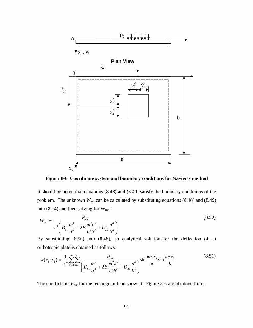
p00
x3, w
x2
2c
2c
2d
2d
0 ξ1
ξ2
a
b
Plan View
Figure 8-6 Coordinate system and boundary conditions for Navier’s method
It should be noted that equations (8.48) and (8.49) satisfy the boundary conditions of the
problem. The unknown Wmn can be calculated by substituting equations (8.48) and (8.49)
into (8.14) and then solving for Wmn:
P (8.50)mnW = mn 4 2 2 4m n n π 4 D11
m + 2Ba b 2 + D22 b4 4 2a
By substituting (8.50) into (8.48), an analytical solution for the deflection of an
orthotropic plate is obtained as follows:
mn( , x ) = 1 ∞ ∞ P sin mπ x1 sin nπ x2
(8.51) π
w x1 2 4 ∑∑ 4 2 2 n4 a bm=1 n=1 D11
m 4 + 2B m n
+ D22 b4 2 a a b 2
The coefficients Pmn for the rectangular load shown in Figure 8-6 are obtained from:
127
4 p0 ξ +d / 2 ξ1 +c / 2 mπ x1 nπ x2 dx dx 2
(8.52)P = sin sin mn ∫ξ
2
+d / 2 ∫ξ +c / 2 a b 1 2 1ab
The displacement w(x1,x2) is found by evaluating equation (8.52) and substituting the
obtained Pmn into equation (8.51). The expressions for the moments are obtained by
substituting w(x1,x2) into equation (8.10).
The solution for the deflection of an isotropic plate can be found from equation
(8.51) by having D11 = D22 = D.
8.3 Analytical Results
Version 4 of the program Mathematica is used to evaluate the Levi’s and Navier’s
solutions for the deflection and internal forces in a honeycomb panel that has the same
cross section as the test panel. The coordinates and boundary conditions used in the
Levi’s solution are shown in Figure 8-5 and those for the Navier’s solution are shown in
Figure 8-6. The boundary conditions are not exactly the same as those in the test panel
for the sake of simplicity. To evaluate the effect of the material orthotropy, the solutions
for orthotropic and isotropic plates are compared. The orthotropic solution uses the
material properties given in Table 8-1, and the isotropic solution uses only the elastic
modulus in the direction x1 given in Table 8-1.
8.3.1 Results from Levi’s solution
For this analysis, the dimensions of the loading area are assumed to be 12x12 in.
The span is 48.5 in. The maximum displacement at the center of the panel (i.e. at
x1=24.25 in. and x2=0 in. in Figure 8-5) due to a load of 26 kips is obtained with equation
(8.46) for the orthotropic plate and with equation (8.35) for the isotropic plate. Strictly
speaking, equations (8.46) and (8.35) are only applicable to plate deflection outside the
loading area. However, the dimensions of the loading area are small compared to the
overall plate dimensions. For this reason, this limitation is ignored here. The Levi’s
solution converges extremely rapidly. The difference in displacement by using five terms
128
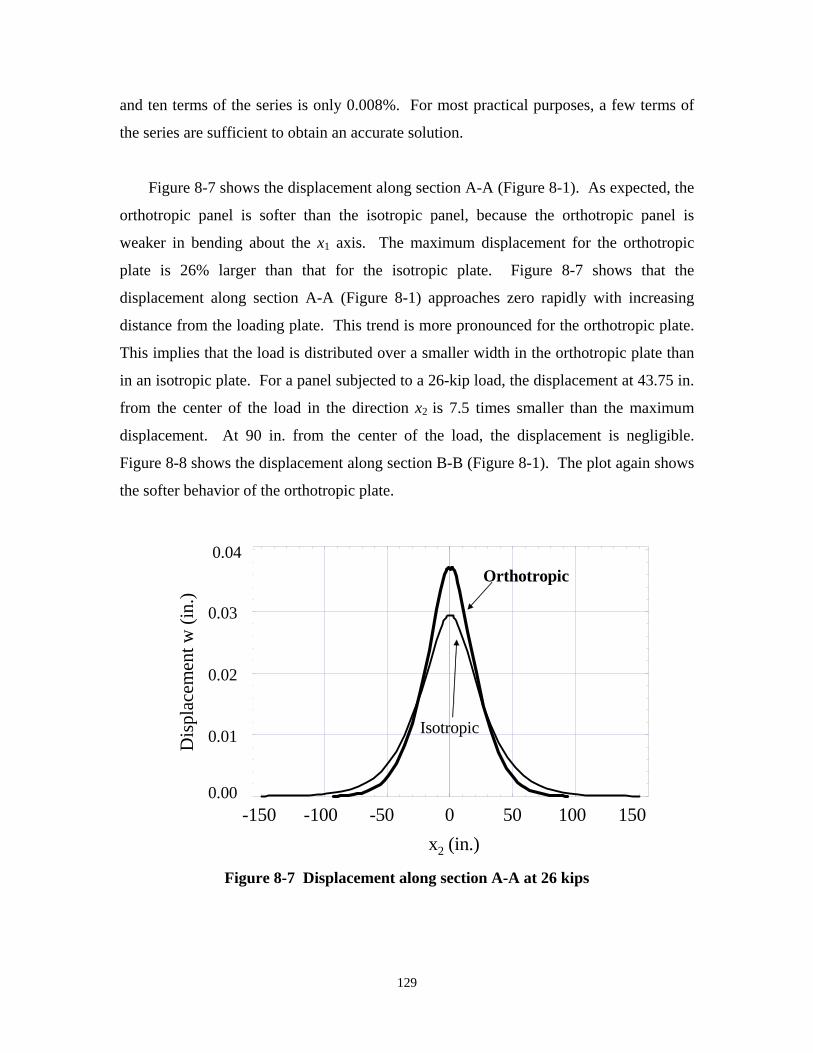
-150 -100 -50 0 50 100 150
0.005
0.01
0.015
0.02
and ten terms of the series is only 0.008%. For most practical purposes, a few terms of
the series are sufficient to obtain an accurate solution.
Dis
plac
emen
t w (i
n.)
Figure 8-7 shows the displacement along section A-A (Figure 8-1). As expected, the
orthotropic panel is softer than the isotropic panel, because the orthotropic panel is
weaker in bending about the x1 axis. The maximum displacement for the orthotropic
plate is 26% larger than that for the isotropic plate. Figure 8-7 shows that the
displacement along section A-A (Figure 8-1) approaches zero rapidly with increasing
distance from the loading plate. This trend is more pronounced for the orthotropic plate.
This implies that the load is distributed over a smaller width in the orthotropic plate than
in an isotropic plate. For a panel subjected to a 26-kip load, the displacement at 43.75 in.
from the center of the load in the direction x2 is 7.5 times smaller than the maximum
displacement. At 90 in. from the center of the load, the displacement is negligible.
Figure 8-8 shows the displacement along section B-B (Figure 8-1). The plot again shows
the softer behavior of the orthotropic plate.
0.04
0.03
0.02
0.01
0.00
Orthotropic
Isotropic
x-150 -100 -50 0 50 100 150
2 (in.)
Figure 8-7 Displacement along section A-A at 26 kips
129

0 10 20 30 40
0.005
0.01
0.015
0.020.04
0.03
Dis
plac
emen
t w (i
n.)
0.02
0.01
0.00
Orthotropic
Isotropic
x
0 10 20 30 40 48.5
1 (in.)
Figure 8-8 Displacement along section B-B at 26 kips
Although the Levi’s solution converges extremely fast, it requires very involved
mathematical manipulation. This is especially true for the case of orthotropic plates. In
addition, the calculation of the derivative of the displacement, which are required to find
the internal moments and forces, exhibits convergence problems in vicinity of the center
of the load. This is probably due to the fact that equations (8.46) and (8.35) are not valid
in the loading area. The Navier’s solution is less general and converges less rapidly than
the Levi’s solution. However, the Navier’s method involves simpler mathematical
manipulation and the solution found can be used for calculating the plate internal forces
in the loaded region. For this reason, the Navier’s solution is used to calculate the
internal forces and the results are presented in the next section.
8.3.2 Results from Navier’s solution
The panel is assumed to be simply supported along four edges. Szilard (1974)
claims that the convergence of this solution is relatively fast provided that the ratios a/c
and d/b (where a, b, c and d are shown in Figure 8-6) are small. Here, a is 48.5 in., d and
c are assumed to be 12 in. and b is assumed to be 10 times a. Further increase of b does
not lead to a noticeable change of the results. The aim is to simulate a finitely long panel
130
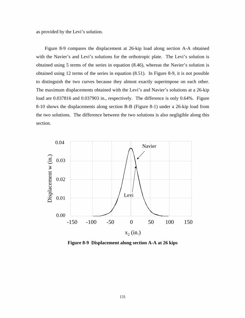
-150 -100 -50 0 50 100 150
0.005
0.01
0.015
0.02
as provided by the Levi’s solution.
Figure 8-9 compares the displacement at 26-kip load along section A-A obtained D
ispl
acem
ent w
(in.
) with the Navier’s and Levi’s solutions for the orthotropic plate. The Levi’s solution is
obtained using 5 terms of the series in equation (8.46), whereas the Navier’s solution is
obtained using 12 terms of the series in equation (8.51). In Figure 8-9, it is not possible
to distinguish the two curves because they almost exactly superimpose on each other.
The maximum displacements obtained with the Levi’s and Navier’s solutions at a 26-kip
load are 0.037816 and 0.037903 in., respectively. The difference is only 0.64%. Figure
8-10 shows the displacements along section B-B (Figure 8-1) under a 26-kip load from
the two solutions. The difference between the two solutions is also negligible along this
section.
0.04
0.03
0.02
0.01
0.00
Levi
Navier
x
-150 -100 -50 0 50 100 150
2 (in.)
Figure 8-9 Displacement along section A-A at 26 kips
131

0 10 20 30 40
0.005
0.01
0.015
0.020.04
0.03D
ispl
acem
ent w
(in.
)
0.02
0.01
0.00
Navier
Levi
x
0 10 20 30 40 48.5
1 (in.)
Figure 8-10 Displacement along section B-B at 26 kips
The three dimensional plot shown in Figure 8-11 obtained with the Navier’s
solution emphasizes the fact that the displacement for the orthotropic plate decreases to
zero very rapidly with increasing distance from the center of the load. Figure 8-12 and
Figure 8-13 show the displacements obtained with the Navier’s solution along section A
A and section B-B (Figure 8-1) of a panel subjected to a load of 26 kips. The maximum
displacements under a load of 26 kips are 0.0379 in. and 0.0303 in. for the orthotropic
plate and the isotropic plate, respectively.
132

133
010
2030
40
24.25
-100
0
100
x2
0
0.005
0.01
0.015
0.02
x3
0
0.005
0.01
0.015
0.02
x3
0.03
0.02
0.04
0 10 2030
40x1
x3,w
-100
0
0.01
0.00100x2
010
2030
40
24.25
-100
0
100
x2
0
0.005
0.01
0.015
0.02
x3
0
0.005
0.01
0.015
0.02
x3
0.03
0.02
0.04
0 10 2030
40x1
x3,w
-100
0
0.01
0.00100x2
Figure 8-11 3D plot of the displacement at 26 kips
-150 -100 -50 0 50 100 150
0.005
0.01
0.015
0.02
-150 -100 -50 0 50 100 150
0.03
0.02
0.01
0.00
0.04
x2 (in.)
Dis
plac
emen
t w (i
n.)
Orthotropic
Isotropic
Figure 8-12 Displacement along section A-A at 26 kips
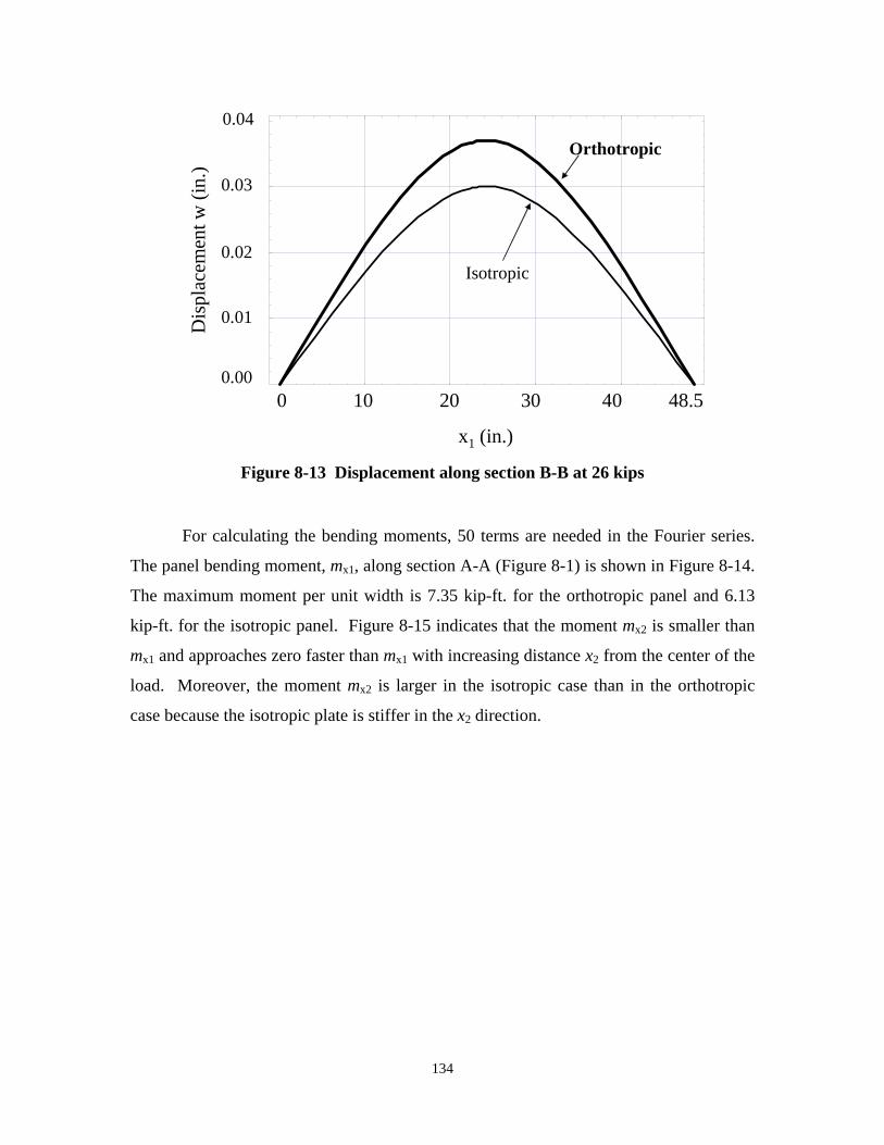
0 10 20 30 40
0.005
0.01
0.015
0.020.04
0.03 D
ispl
acem
ent w
(in.
)
0.02
0.01
0.00
Orthotropic
Isotropic
x
0 10 20 30 40 48.5
1 (in.)
Figure 8-13 Displacement along section B-B at 26 kips
For calculating the bending moments, 50 terms are needed in the Fourier series.
The panel bending moment, mx1, along section A-A (Figure 8-1) is shown in Figure 8-14.
The maximum moment per unit width is 7.35 kip-ft. for the orthotropic panel and 6.13
kip-ft. for the isotropic panel. Figure 8-15 indicates that the moment mx2 is smaller than
mx1 and approaches zero faster than mx1 with increasing distance x2 from the center of the
load. Moreover, the moment mx2 is larger in the isotropic case than in the orthotropic
case because the isotropic plate is stiffer in the x2 direction.
134

-100 -50 0 50 100
0
2000
4000
6000
8000
-100 -50 0 50 100
0
2000
4000
6000
8000
2
0
mx1
(kip
s-ft)
Orthotropic
Isotropic
4
6
8
mx2
(kip
s ft)
x-100 -50 0 50 100
2 (in.)Figure 8-14 Moment mx1 along section A-A at 26 kips
8
6
x
4
2
0
-100 -50 0 50 100
2 (in.)
Orthotropic
Isotropic
Figure 8-15 Moment mx2 along section A-A at 26 kips
135

The next section presents a parametric study performed using the Navier’s
method to determine the effective bending width for the GFRP sandwich panel
considered here.
8.4 Effective Bending Width
8.4.1 Introduction
In this section, the Navier’s solution is used for a parametric study to determine the
effective bending width for several GFRP panels with different geometries.
The effective bending width used here is defined by Szilard (1974). According to
this definition, the effective width b’ for the bending of a plate is obtained by equating
the actual moment area for mx1 with that of a fictitious rectangular moment diagram that
has the same maximum moment as mx1 as shown in Figure 8-16.
x2
x1
a
0
mx1
mx1
b
b’
d
c
a/2
b/2
loading area
a/2
b/2
Figure 8-16 Effective bending width
Using the above definition, the effective bending width b’ is given by the following
formula:
136
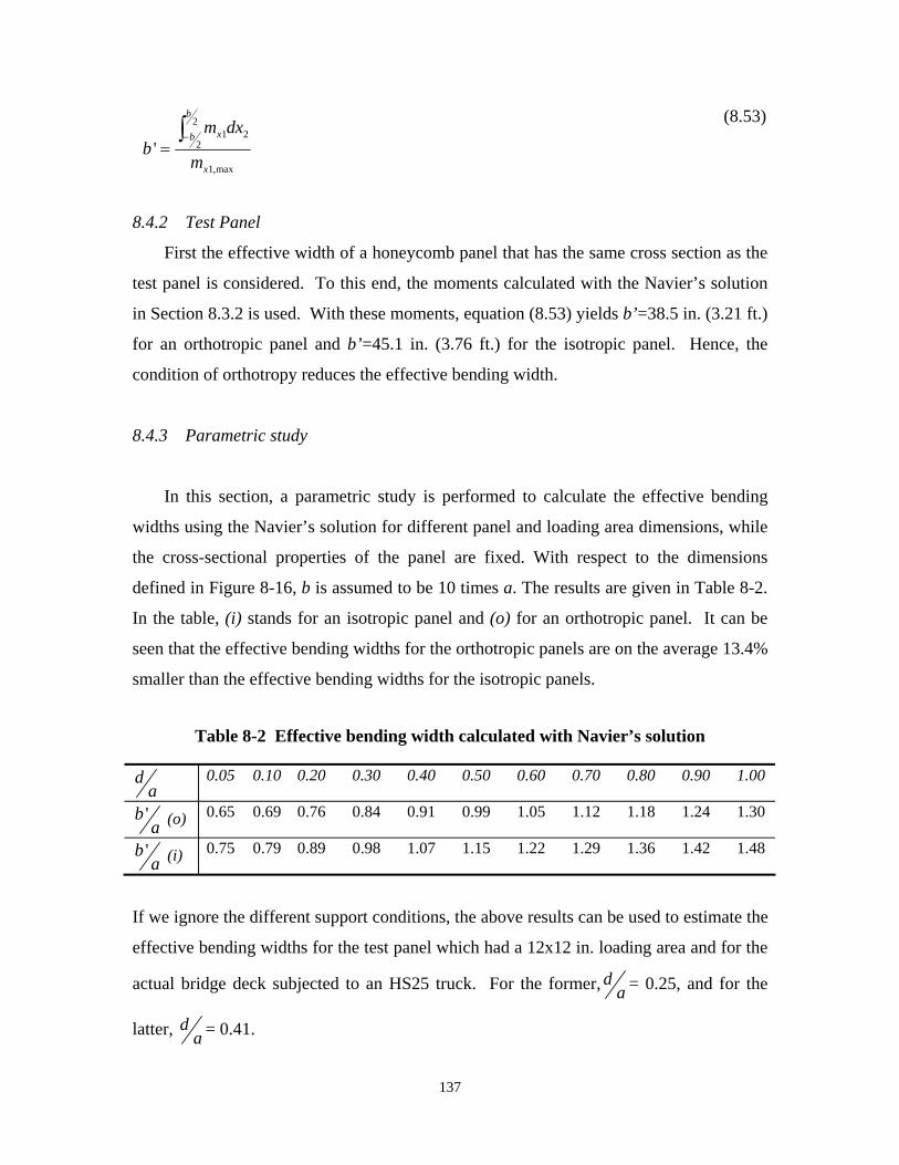
(8.53) 2
b m dx 2x1∫−
2 b
b ' = mx1,max
8.4.2 Test Panel
First the effective width of a honeycomb panel that has the same cross section as the
test panel is considered. To this end, the moments calculated with the Navier’s solution
in Section 8.3.2 is used. With these moments, equation (8.53) yields b’=38.5 in. (3.21 ft.)
for an orthotropic panel and b’=45.1 in. (3.76 ft.) for the isotropic panel. Hence, the
condition of orthotropy reduces the effective bending width.
8.4.3 Parametric study
In this section, a parametric study is performed to calculate the effective bending
widths using the Navier’s solution for different panel and loading area dimensions, while
the cross-sectional properties of the panel are fixed. With respect to the dimensions
defined in Figure 8-16, b is assumed to be 10 times a. The results are given in Table 8-2.
In the table, (i) stands for an isotropic panel and (o) for an orthotropic panel. It can be
seen that the effective bending widths for the orthotropic panels are on the average 13.4%
smaller than the effective bending widths for the isotropic panels.
Table 8-2 Effective bending width calculated with Navier’s solution
d a
0.05 0.10 0.20 0.30 0.40 0.50 0.60 0.70 0.80 0.90 1.00
'b a (o) 0.65 0.69 0.76 0.84 0.91 0.99 1.05 1.12 1.18 1.24 1.30
'b a (i) 0.75 0.79 0.89 0.98 1.07 1.15 1.22 1.29 1.36 1.42 1.48
If we ignore the different support conditions, the above results can be used to estimate the
effective bending widths for the test panel which had a 12x12 in. loading area and for the
actual bridge deck subjected to an HS25 truck. dFor the former, = 0.25, and for thea
latter, d = 0.41.a
137

EQUATION CHAPTER 9 SECTION 1
9 FINITE ELEMENT ANALYSES OF TEST PANEL
9.1 Introduction
As mentioned in Section 8.1, the Kirchhoff-Love theory gives accurate results only
if the ratio of the smallest lateral dimension of the plate to its thickness is at least ten. To
obtain a more accurate assessment of the behavior of the test panel and to account for the
actual boundary conditions used in the test, the panel is analyzed with the finite element
method (FEM) in this chapter. The finite element analysis (FEA) considers the loading
conditions of the initial static test, i.e., with the two spans of the panel loaded
simultaneously. To exploit the symmetry condition of the two-span test panel, only one
span is considered and the panel is assumed to be fixed along one edge, simply supported
along the opposite edge, and free along the other two edges in the FEA.
9.2 Model Description
Finite element analyses are performed with a 3D mesh using Version 6-3.1 of the
program ABAQUS. Two types of 3D models are developed for this purpose. The panel
model has a span of 48.5 in. (center-to-center distance of the risers in the original test
panel) and a width of 100 in.
The first model, Model A, uses 8-node quadratic thick-shell elements. The boundary
conditions and mesh discretization are shown in Figure 9-1. Except for the shear moduli,
the whole panel is modeled with the equivalent orthotropic material properties of a
homogenized sandwich panel as presented in Table 8-1. The thick shell element
implemented in ABAQUS accounts for the shear deformation. The shear moduli, G13
and G23, are assumed to be the core shear moduli shown in Table 3-2. Model A is very
simple and computationally very efficient. Consequentially, it is useful for parametric
studies to determine the effective bending widths of a panel under different geometric
and boundary conditions. Nevertheless, it is not capable of calculating the interface shear
stresses between the face and the core of a panel. These stresses can cause debonding
138

failure, and are, therefore, important to evaluate.
Fix boundary
Simply supported boundary
Figure 9-1 Boundary conditions and mesh discretization for Model A
For the above reason, a second model, Model B, is also considered. The boundary
conditions and mesh discretization are shown in Figure 9-2. This model distinguishes the
three distinct layers of a panel, i.e. the two faces and the core. The material properties for
each layer are given in Table 3-2. The core is modeled using four layers of 20-node
quadratic brick elements. The faces are modeled with 8-node quadratic shell elements.
The shell elements are connected to the brick elements using the tie option of the
program.
Fix boundary
Simply supported boundary
Bottom shell
Top shell
Brick elements
Figure 9-2 Boundary conditions and mesh discretization for Model B
139
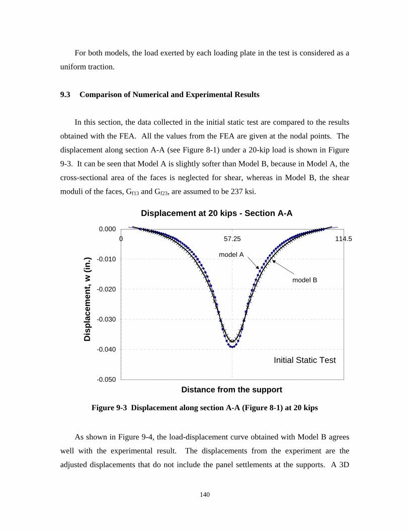
Distance from the center of the load
For both models, the load exerted by each loading plate in the test is considered as a
uniform traction.
Dis
plac
emen
t, w
(in.
) 9.3 Comparison of Numerical and Experimental Results
In this section, the data collected in the initial static test are compared to the results
obtained with the FEA. All the values from the FEA are given at the nodal points. The
displacement along section A-A (see Figure 8-1) under a 20-kip load is shown in Figure
9-3. It can be seen that Model A is slightly softer than Model B, because in Model A, the
cross-sectional area of the faces is neglected for shear, whereas in Model B, the shear
moduli of the faces, Gf13 and Gf23, are assumed to be 237 ksi.
Displacement at 20 kips - Section A-A
0.000
-0.010
-0.020
-0.030
-0.040
-0.050
0
Initial Static Test
model B
model A
57.25 114.5
Distance from the support
Figure 9-3 Displacement along section A-A (Figure 8-1) at 20 kips
As shown in Figure 9-4, the load-displacement curve obtained with Model B agrees
well with the experimental result. The displacements from the experiment are the
adjusted displacements that do not include the panel settlements at the supports. A 3D
140
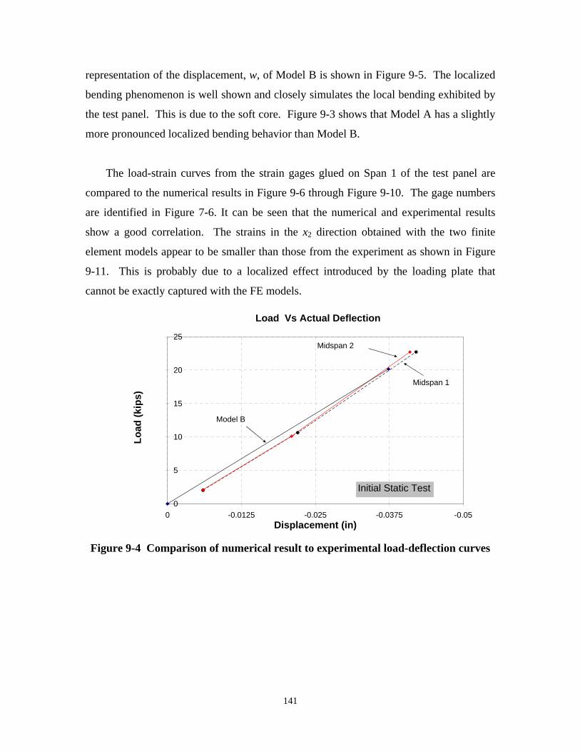
representation of the displacement, w, of Model B is shown in Figure 9-5. The localized
bending phenomenon is well shown and closely simulates the local bending exhibited by
the test panel. This is due to the soft core. Figure 9-3 shows that Model A has a slightly
more pronounced localized bending behavior than Model B.
The load-strain curves from the strain gages glued on Span 1 of the test panel are
compared to the numerical results in Figure 9-6 through Figure 9-10. The gage numbers
are identified in Figure 7-6. It can be seen that the numerical and experimental results
show a good correlation. The strains in the x2 direction obtained with the two finite
element models appear to be smaller than those from the experiment as shown in Figure
9-11. This is probably due to a localized effect introduced by the loading plate that
cannot be exactly captured with the FE models.
Load Vs Actual Deflection
0
5
10
15
20
25
Load
(kip
s)
Initial Static Test
Midspan 2
Midspan 1
Model B
0 -0.0125 -0.025 -0.0375 -0.05 Displacement (in)
Figure 9-4 Comparison of numerical result to experimental load-deflection curves
141

x2
x1
x3,w
Fix boundary
Simply supported boundary
Load
(kip
s)
Figure 9-5 3D plot of the displacement at 20 kips (Model B)
Load vs strain (ε11) under the load 1
25
20
15
10
5
0 -0.0009 -0.0006 -0.0003 0 0.0003 0.0006 0.0009
BA BA
Gage 10
BOTTOM STRAIN TOP STRAIN
Gage 1
Strain
Figure 9-6 Load-strain (ε11) curves of the gages under load 1
142

Load vs strain (ε11) at 9 in. from load 1
0
5
10
15
20
25
Load
(kip
s) B
A B
A
BOTTOM STRAIN TOP STRAIN
Gage 6 Gage 12
-0.0009 -0.0006 -0.0003 0 0.0003 0.0006 0.0009
Strain
Figure 9-7 Load-strain (ε11) curves at 9 in. from load 1
Load vs strain ( ) at 17.5 in. from load 1ε11
0
5
10
15
20
25
Load
(kip
s)
B
A B
A
Gage 13
BOTTOM STRAIN TOP STRAIN
Gage 7
-0.0009 -0.0006 -0.0003 0 0.0003 0.0006 0.0009
Strain
Figure 9-8 Load-strain (ε11) curves at 17.5 in. from load 1
143
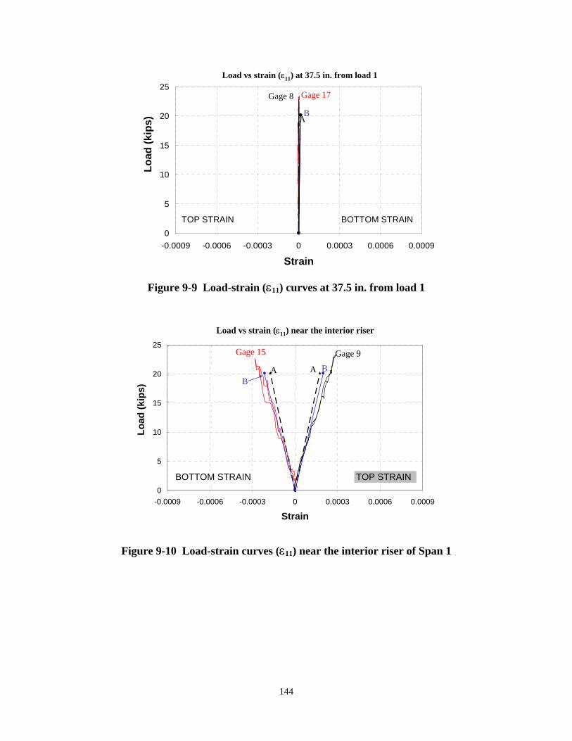
Load vs strain ( ) at 37.5 in. from load 1ε11
0
5
10
15
20
25
Load
(kip
s)
Gage 8 Gage 17
AB
BOTTOM STRAIN TOP STRAIN
-0.0009 -0.0006 -0.0003 0 0.0003 0.0006 0.0009
Strain
Figure 9-9 Load-strain (ε11) curves at 37.5 in. from load 1
Load vs strain ( ) near the interior riser ε11
0
5
10
15
20
25
Load
(kip
s)
Gage 15 Gage 9
BAA B
BOTTOM STRAIN TOP STRAIN
-0.0009 -0.0006 -0.0003 0 0.0003 0.0006 0.0009
Strain
Figure 9-10 Load-strain curves (ε11) near the interior riser of Span 1
144
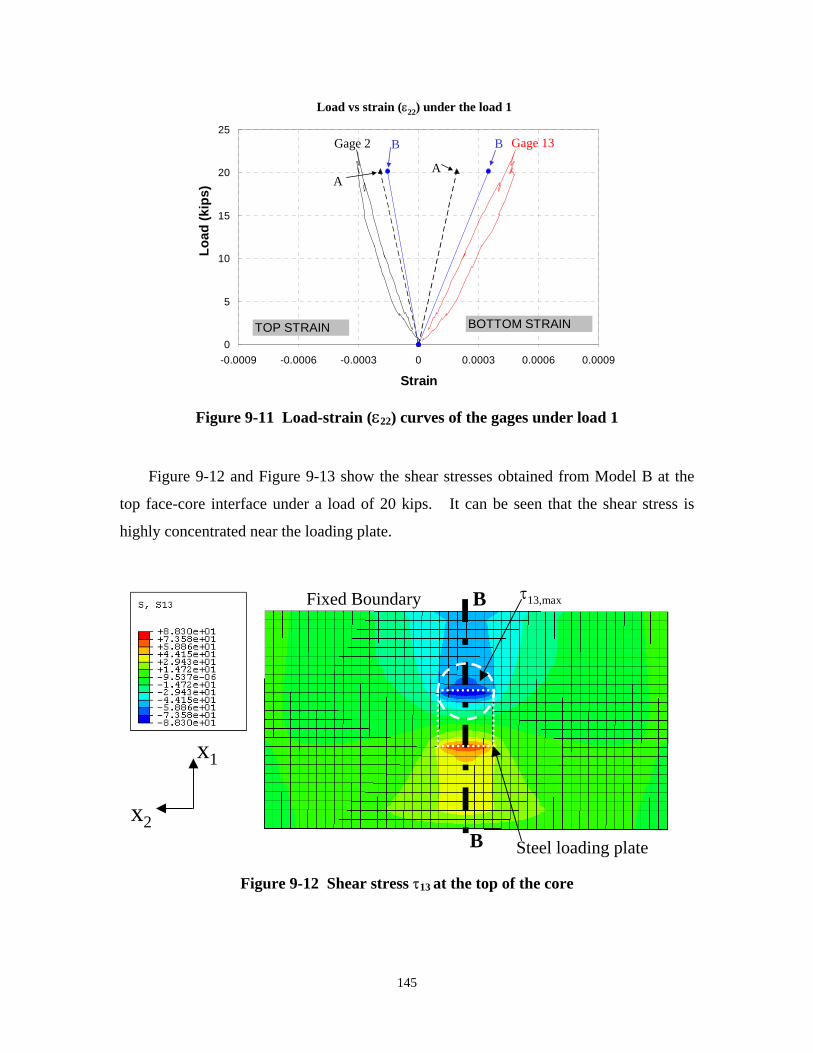
Load vs strain ( ) under the load 1ε22
25
20
Load
(kip
s)15
10
5
0 -0.0009 -0.0006 -0.0003 0 0.0003 0.0006 0.0009
Gage 2 B
A
B
A
Gage 13
BOTTOM STRAIN TOP STRAIN
Strain
Figure 9-11 Load-strain (ε22) curves of the gages under load 1
Figure 9-12 and Figure 9-13 show the shear stresses obtained from Model B at the
top face-core interface under a load of 20 kips. It can be seen that the shear stress is
highly concentrated near the loading plate.
B
B x2
x1
Steel loading plate
τFixed Boundary 13,max
Figure 9-12 Shear stress τ13 at the top of the core
145
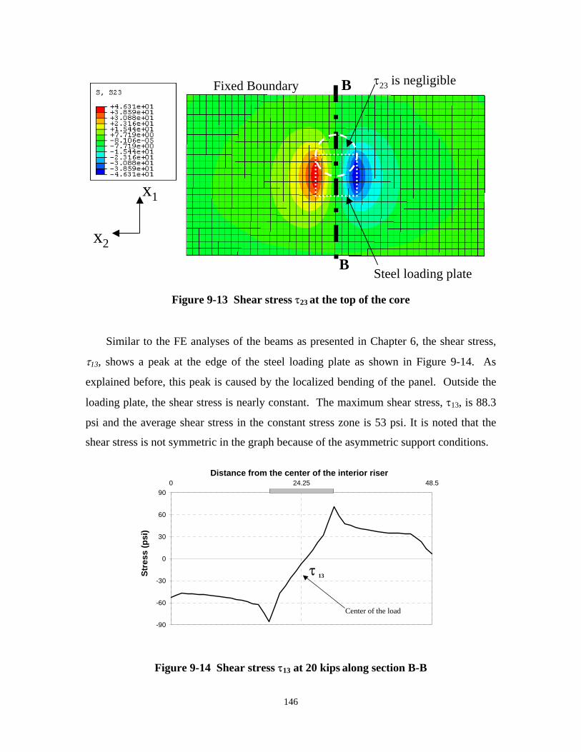
Fixed Boundary
x2
x1
Steel loading plate
B
B
τ23 is negligible
Figure 9-13 Shear stress τ23 at the top of the core
Similar to the FE analyses of the beams as presented in Chapter 6, the shear stress,
τ13, shows a peak at the edge of the steel loading plate as shown in Figure 9-14. As
explained before, this peak is caused by the localized bending of the panel. Outside the
loading plate, the shear stress is nearly constant. The maximum shear stress, τ13, is 88.3
psi and the average shear stress in the constant stress zone is 53 psi. It is noted that the
shear stress is not symmetric in the graph because of the asymmetric support conditions.
Distance from the center of the interior riser 0 24.25 48.5
Stre
ss (p
si)
90
60
30
0
-30
-60
-90
τ 13
Center of the load
Figure 9-14 Shear stress τ13 at 20 kips along section B-B
146

9.3.1 Distribution of Interface Shear
The shear stress at the interface between a face and the core triggers the delamination
failure and, consequentially, its distribution is important to examine. Model B can be
used to calculate the interface shear stress between the core and a face. The boundary
conditions and dimensions of the panel considered here are the same as those of the test
panel. Figure 9-15 shows the shear stress τ13 from the FEA at the top face-core interface
under a load of 20 kips. The figure indicates that the shear stress decreases very quickly
away from the load. At about 25 in. from the center of the load, the shear stress τ13 is
11% of τ13,max, and it goes to zero at about 43 in. from the center of the load.
1% τ 11% τ
τ 61% τ
τ
T T x2
x113, max
13, max
31% 13, max
13, max
13, max=88.3 psi
Figure 9-15 Shear stress τ13 at the top of the core
9.4 Comparison of the Shear Strengths of the Test Beams and Test Panel
Similar to the beam tests reported in Chapter 5, the panel test shows that the
governing failure mode of the panel is the delamination of the face from the core. The
interface shear strengths of the beams estimated from the test results using different
methods are shown in Table 6-1. As shown in Table 6.1, the average interface shear
147
stresses at failure in the constant shear zone estimated with the FEA were 380 psi for Test
1, 310 psi for Test 2, 190 psi for Test 3, and 550 psi for Test 4. Thus, the average shear
strength of all four beams was 357 psi. At a load of 20 kips, the average interface shear
stress in the constant shear zone of the panel obtained from the FEA is 53 psi, which is
15% of the average shear stress of the beams at failure.
In phase 1 of the fatigue test (from 0 to 15,000 cycles), the panel was loaded to a
maximum load of 40 kips. At 40 kips, the interface shear stress in the shear span is
estimated to be 106 psi according to the above FEA, which is 30% of the average shear
strength of the beams. This is a very low value and it is not expected to induce
debonding under the limited number of fatigue load cycles. Therefore, the premature
delamination of the test panel in Span 2 during the initial fatigue load cycles was most
likely caused by defects introduced in the fabrication process. This is confirmed by the
fact that no delamination occurred in Span 1 during these cycles.
After 1.5 million load cycles, Span 1 delaminated at a static load of 62 kips as shown
in Figure 7-28. Under a load of 62 kips, the interface shear stress in the constant shear
zone of Span 1 is estimated to be 164 psi according to the FEA.
It is well known that GFRP has a lower fatigue resistance than Carbon and Aramid
FRP. ACI 440 (2000) suggests that stresses in GFRP materials be limited to 20% of the
ultimate strength under service load conditions. Nevertheless, no information is available
with regard to the fatigue endurance of the face-core interface.
9.5 Effective Bending Width
9.5.1 Introduction
The analytical results from the plate theory show that the effective bending width of
an orthotropic panel is 13.4% smaller than that of an isotropic panel. However, the
analytical solution only considers simple boundary conditions and does not consider the
shear deformation of the soft core. This section presents a study performed with finite
148

element analysis to determine how the panel boundary conditions and the shear
deformation affect the effective bending width. The numerical result is used to determine
the effective bending width and compare with that obtained from the test data and that
used in the preliminary design evaluation in Chapter 4.
Model A is used here because it is very simple and computationally efficient, and,
consequentially, more suitable for parametric studies. The material properties of the
panel are given in Table 8-1. The shear deformation of the panel is taken into account by
using the shear moduli of the core given in Table 3-2.
9.5.2 Test Panel
Figure 9-16 shows the moment mx1 at nodal points along section A-A (as identified
in Figure 8-1) for a panel subjected to a load of 20 kips.
Center of the load
Mom
ent,
mx1 (k
ips
ft)
5
4
3
2
1
0
0 28.625 57.25 85.875 114.5 x2 (in.)
Figure 9-16 Moment mx1 along section A-A
The maximum moment per unit width, mx1, calculated with the finite element
model is 4.73 kips-ft. Using calculated moments along section A-A, equation (8.53)
gives an effective bending width, b’, of 27.9 in. (2.33 ft.). In order to compare the
149
theoretical effective bending width with the experimental value, the plane section
remaining plane assumption is used to calculate the bending moment from the
experimental strain measurements. Accordingly, the substitution of equation (8.7) into
(8.9) leads to H E11 (ε +υ ε )x dx
(9.1) 11 21 22 3 3mx1 = ∫−H
2
2 1 −υ υ12 21
υ21 = υ E11 (9.2)12 E22
At a load of 20 kips, the maximum strains ε11 and ε22 at the bottom of Span 1 of the
test panel were 0.000302 and 0.000439, respectively. By assuming a linear strain
distribution along the depth of the panel and using the material properties in Table 8-1, it
is possible to integrate equation (9.1) and evaluate the maximum moment:
1273000 3.75 0.000302 0.000439 = 3 3mx1,max 1 − 0.301× 0.189 ∫−3.75
( 3.75
x3 + 0.189 3.75
x3) x dx (9.3)
Therefore, the experimental maximum moment per unit width, mx1, is 4.87 kips-ft., which
is only 3% higher than the numerical result.
Equation (9.1) shows that the strains in both directions contribute to the moment mx1,
and, therefore, affect the effective bending width. Substituting equation (9.1) into
equation (8.53), we have: b H
2 2 2 ,( (x x ) +υ ε ( x x ))x dx dx (9.4)
3 21 22 2 , 3 3 3 2∫ ∫−H ε11 −b
2 2b ' ε = H 2max ∫−H (ε ( x2 , x ) +υ ε ( x2, x )) x dx 3
11 3 21 22 3 3along x 2 2
Equation (9.4) expresses the effective bending width as a function of the strains and
Poisson’s ratio. The contribution of the strain in direction x2 is very small for two
reasons. First, in equation (9.1), ε22 is multiplied by the Poisson’s Ratio υ and,21
therefore, its effect is decreased by 81%. Secondly, the FE analysis shows that the
distribution of ε22 is different from that of ε11. ε22 approaches zero extremely quickly and
150
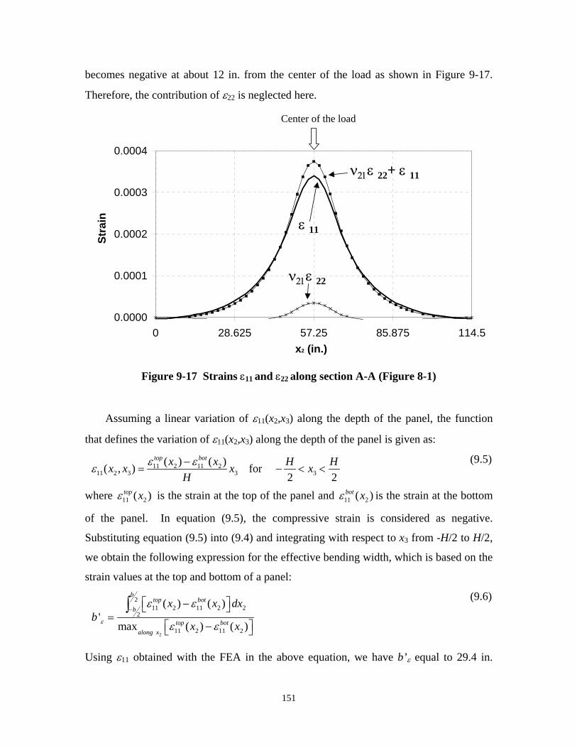
0.0004
becomes negative at about 12 in. from the center of the load as shown in Figure 9-17.
Therefore, the contribution of ε22 is neglected here.
Center of the load St
rain
0.0003
0.0002
0.0001
0.0000
ε 11
ν21ε 22
ν21ε 22+ ε 11
0 28.625 57.25 85.875 114.5 x2 (in.)
Figure 9-17 Strains ε11 and ε22 along section A-A (Figure 8-1)
Assuming a linear variation of ε11(x2,x3) along the depth of the panel, the function
that defines the variation of ε11(x2,x3) along the depth of the panel is given as:
ε ( , top x2
bot ( )x x3) = ε11 ( ) − ε11 x2 H H (9.5) x3 for − < x3 <11 2 H 2 2
top ( ) bot ( )where ε11 x2 is the strain at the top of the panel and ε x2 is the strain at the bottom 11
of the panel. In equation (9.5), the compressive strain is considered as negative.
Substituting equation (9.5) into (9.4) and integrating with respect to x3 from -H/2 to H/2,
we obtain the following expression for the effective bending width, which is based on the
strain values at the top and bottom of a panel:
top bot
2 b 11 ( ) − ε ( ) dx (9.6)ε x2 11 x2 2∫−
2b
b ' ε = top ( x ) − ε bot ( x2 )2 11 max along x 2
ε11
Using ε11 obtained with the FEA in the above equation, we have b’ε equal to 29.4 in.
151
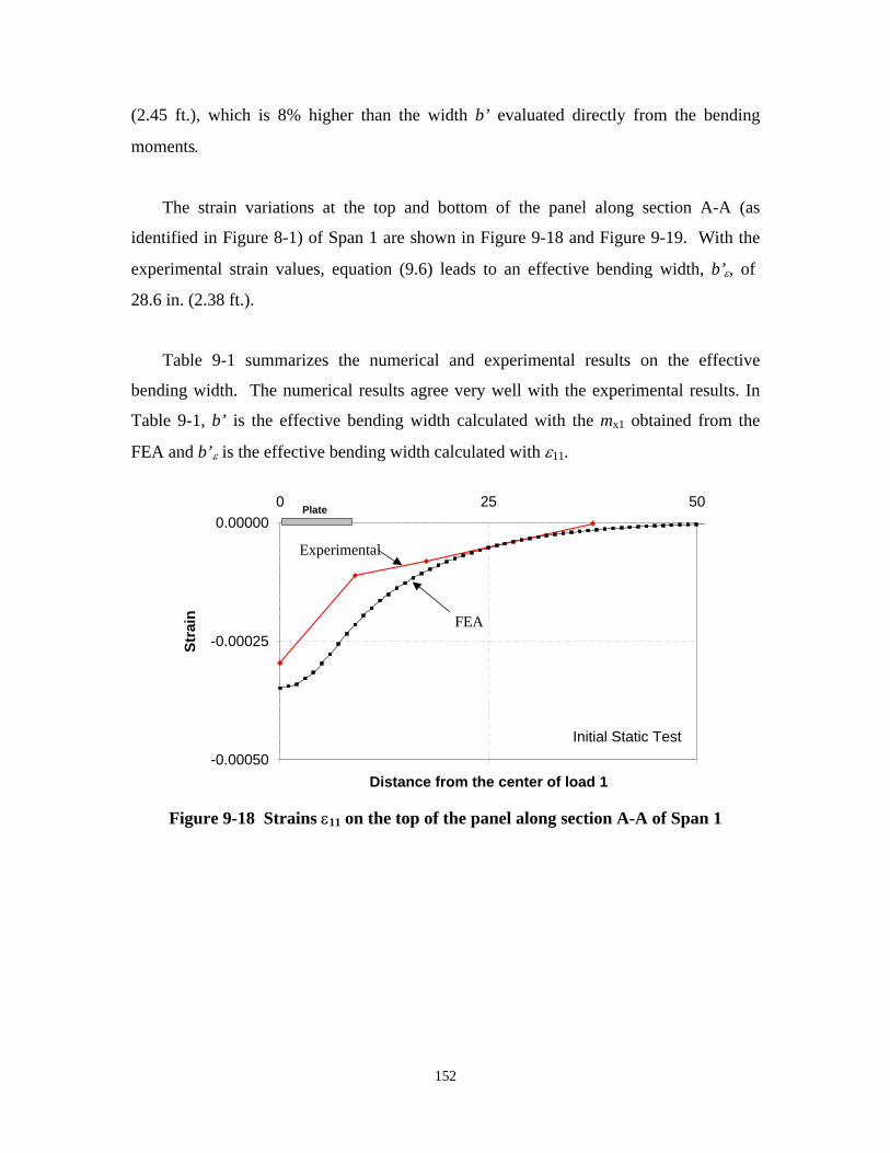
(2.45 ft.), which is 8% higher than the width b’ evaluated directly from the bending
moments.
Stra
in
The strain variations at the top and bottom of the panel along section A-A (as
identified in Figure 8-1) of Span 1 are shown in Figure 9-18 and Figure 9-19. With the
experimental strain values, equation (9.6) leads to an effective bending width, b’ε, of
28.6 in. (2.38 ft.).
Table 9-1 summarizes the numerical and experimental results on the effective
bending width. The numerical results agree very well with the experimental results. In
Table 9-1, b’ is the effective bending width calculated with the mx1 obtained from the
FEA and b’ε is the effective bending width calculated with ε11.
0 25 50 Plate 0.00000
-0.00025
-0.00050
FEA
Initial Static Test
Experimental
Distance from the center of load 1
Figure 9-18 Strains ε11 on the top of the panel along section A-A of Span 1
152

0 25 50 0.0005
Stra
in
0.0003
0.0000 FEA
Initial Static Test
Experimental
Distance from the center of load 1
Figure 9-19 Strains ε11 on the bottom of the panel along section A-A (Figure 8-1) of Span 1
Table 9-1 FE and experimental effective bending widths
b’ (ft.) b’ε (ft.) FEA 2.33 2.45 Experimental 2.38
9.5.3 Parametric Study
This section examines the influence of the panel boundary conditions and the shear
deformation in the soft core on the effective bending width. Instead of using the
dimensions of the loading plates used in the panel test, the actual foot print of a HS25
truck is considered in the analyses. Hence, results of this study can be used as a guidance
for actual design. In the AASHTO LFRD Specifications (1998), the foot print of a wheel
load is assumed to be a rectangle with a width of 20 in. and length l given by:
IM (9.7)l = 2.28γ
1 + 100 P
where γ is the load factor, IM is the dynamic-load allowance, and P is the wheel load.
For the type of truck load and deck considered here, γ is 1.75, IM =30, and P=20 kips.
Therefore, the contact area for the wheel load is 20x19 in. Hence, with respect to Figure
153
8-16, c=20 in. and d=19 in. Furthermore, considering the dimensions of the actual deck,
a is assumed to be 48.5 in. and b is assumed to be 525 in.
Effect of the Shear Deformation
To examine the effect of the shear deformation due to the soft core, we consider a
panel with two opposite edges simply supported and the other two edges free. First, the
panel is analyzed as a thin plate with Model A. The maximum moment per unit width,
mx1, under a load of 20 kips is 4.18 kip-ft. and effective bending width calculated is 3.72
ft. Second, the panel is analyzed as a thick plate. The maximum moment per unit width,
mx1, under a load of 20 kips is 4.81 kip-ft. and the effective bending width calculated is
3.25 ft. The above results show that the effective bending width based on the thick plate
theory is 87% of that based on a thin plate.
To check the results obtained with the Kirchhoff-Love theory in Chapter 8, the
results obtained with the finite element model based on the thin plate assumption are
considered. The maximum moment per unit width, mx1, under a load of 20 kips is 4.18
kip-ft. according to the finite element model and 4.16 kips-ft. according to the Navier’s
solution. The effective bending width calculated with the finite element model is 3.72 ft.
and with the Navier’s method is 3.86 ft. The results show good agreement.
Effect of Boundary Conditions
To examine the influence of the panel boundary conditions, a panel with one edge
fixed, the opposite edge simply supported and the other two edges free is analyzed with
Model A using the thick plate assumption. The maximum moment per unit width, mx1,
under a load of 20 kips is 3.67 kip-ft. and the calculated effective bending width is 2.86
ft. Hence, compared to the previous results of a simply supported panel, fixing one edge
reduces the effective bending width by 11%.
Furthermore, a panel with two opposite edges fixed and the other two free is loaded
154
with a load of 20 kips. The maximum moment per unit width, mx1, is 2.24 kip-ft. and the
effective bending width is 2.69 ft. In this case, the effective bending width is 17%
smaller than that of a simply supported panel.
9.5.4 Evaluation of Design Assumptions on Effective Widths
Effective Bending Width
The effective bending width assumed in the design evaluation in Chapter 4 is 4 ft.,
while that obtained from the finite element analysis is 2.86 ft. (Section 9.5.3). However,
the design is still conservative because the evaluation was based on a point load at
midspan, whereas, in reality, the panel is loaded with a truck wheel of finite dimensions.
Furthermore, the design evaluation was based on simply supported boundary conditions,
whereas the FEA considers one side fixed and the other simply supported.
For a simply supported panel subjected to the design wheel load of 26 kips, assuming
a point load and an effective bending width, b’, of 4 ft. leads to a design moment of 6.6
kip-ft. Based on the finite element analysis, for a panel fixed on one side and simply
supported on the other three, the maximum bending moment per unit width is 4.8 kip-ft.
Therefore, the design of the panel is conservative.
Effective Width for Shear
The effective shear width, ws, was assumed to be 7 ft. in the design evaluation in
Chapter 4. The shear stress at the interface between the face and the core for a 7-ft.-wide
strip can be calculated with equation (4.20) by assuming b=ws. For a beam subjected to a int load of 26 kips, equation (4.20) gives an interface shearτ of 22 psi. The shear stress13
has been calculated with finite element analysis using Model B for a load of 26 kips and a
loading area equal to the foot print of an HS25 truck. In the constant shear zone, the
interface shear stress obtained is 49 ksi, which is 2.2 times the shear stress assumed in the
design evaluation. Hence, the effective shear width should be 3.1 ft., with which
155

int equation (4.20) will lead to an interface shear τ of 49 psi.13
In spite of the above observation, the shear strength assumed initially is very
conservative. The shear strengthening detail introduced by Kansas Structural Composites,
Inc. (KSCI) has increased the interface shear strength significantly. The shear strength of
the weakest beam tested was 160 psi as shown in Table 6-2, while the shear strength
assumed in the design evaluation is 80 psi. Using a shear strength of 160 psi and an
effective width of 3.1 ft., equation (4.21) leads to an Ultimate Shear Load Capacity, Ps, of
133 kips. This satisfies the design requirement in that 45% of Ps is higher than the
maximum factored load of 56.5 kips. Considering a service wheel load of 26 kips, the
factor of safety against delamination failure is about 5.
Furthermore, the panel test results indicate that the panel continued to carry
additional load after delamination had first occurred. This is because of the redistribution
of the shear stress in the panel.
Design Considerations
The finite element analyses indicate that the deflection and bending stress
requirements can be easily met by the GFRP panel. However, past research as well as
results of this study shows that the load carrying capacity of GFRP sandwich panels is
governed by the interface shear strength between the core and the faces. Even if the
bending stress is low compared to the tensile strength of the material, the panel might be
unsafe because the level of the interface shear stress could be too high compared to the
interface shear strength.
Currently, the design of this type of panels does not explicitly account for the
interface shear strength and, in particular, the fatigue endurance of the interface bond.
Hence, improved design provisions that account for the interface shear should be
developed. Nevertheless, little information is available with respect to the fatigue
endurance at the face-core interface. In view of this, it is suggested that the interface
156

shear stress be limited to 20% of the interface shear strength under service loads, as
suggested by ACI 440 (2000) to prevent the creep rupture or fatigue failure of GFRP bars
in general. Furthermore, to ensure a consistent shear strength, good quality control
should be exercised in the manufacturing process.
157
10 SUMMARY AND CONCLUSIONS
10.1 Summary
In this report, the design and load-carrying capacity of the glass fiber reinforced
polymer (GFRP) deck on the O’Fallon Park bridge have been evaluated. The deck panels
were manufactured and installed by Kansas Structural Composites, Inc. (KSCI). The
studies conducted here include the laboratory evaluation of the strengths and stiffness of
four GFRP beams, the crushing capacities of panel specimens, and the strength, stiffness,
and fatigue endurance of a full-size two-span continuous deck specimen. Furthermore,
the test results obtained are used to validate analytical and finite element models, which
have been developed to yield general design recommendations.
The deck design was based on the 16th Edition of the AASHTO Specifications
(1996), the AASHTO LFRD Specifications (1998), past research data, and the special
provisions stipulated in the contractual document of the City and County of Denver
(2002).
Four beams were tested to evaluate the influence of the face thickness on the load
resisting behavior of a beam. The beams had a sandwich construction with top and
bottom faces and a 6.5-in.-high honeycomb core. Three of them were 13-in. wide and one
12-in. wide. The latter was due to manufacturing irregularity. Two had a face thickness of
0.375 in. and two had 0.500-in. faces. The beams were loaded to failure under a 3-point
bending configuration to evaluate the stiffness and load-carrying capacity.
Four approximately 13x12-in. panel specimens were subjected to compressive loads
to find the ultimate crushing capacity. Manufactured together with the beam specimens,
two crushing-test specimens had a face thickness of 0.375 in. and two had 0.500-in.
faces.
Analyses were conducted using the Timoshento beam theory and finite element
158
models to study the flexural behavior and failure mode of the beams. An interface finite
element model based on nonlinear fracture mechanics was employed to study the
delamination between the faces and the core of a beam at the ultimate load. Based on the
test and analysis results, a panel section was selected by KSCI for the O’Fallon Park
bridge deck.
A full-size, two-span continuous deck panel that was 114.5-in. long, 120-in.wide,
and 7.5-in. thick with 0.375-in. faces was tested under static loads and fatigue load
cycles. The deck specimen had the same design as the O’Fallon Park bridge deck. The
panel was supported on three reinforced concrete risers and anchored to the supports
using mechanical anchor bolts. The aim of the test was to study the load-carrying
capacity and fatigue endurance of the GFRP panel and mechanical anchors. Prior to the
fatigue test, a static test was performed to evaluate the load-resisting behavior of an
undamaged panel. In the fatigue test, the panel was subjected to 1.5 million load cycles
till delamination occurred in both spans. Once the fatigue test was completed, the panel
was loaded each span at a time to failure.
The deck panel has been analyzed using the Kirchhoff-Love plate theory and finite
element models, which have validated with the test results. These analyses are to
investigate the load distribution and determine the effective bending widths of a panel
subjected to the wheel load of an HS 25 truck. The influence of the material orthotropy,
shear deformation, and boundary conditions on the effective width has also been
investigated.
Based on the results of the aforementioned tests and analyses, design
recommendations are provided.
10.2 Conclusions
The following major conclusions can be drawn from the studies conducted here:
159

1. The beam tests have demonstrated that the deflection limit stipulated in the
design provisions of the City and County of Denver (2002) is satisfied.
2. The governing failure mode of all four beams was the delamination of the
upper face from the core. The beams in Tests 1, 2, and 4 failed in a very brittle
manner and that in Test 3 in a ductile-like manner. The ductile-like behavior
was due to premature progressive delamination caused by the poor bonding
between the upper face and the core.
3. The beam tests have shown a very large scatter in the ultimate load capacities.
This high variability is due to the workmanship and it underscores the
importance of quality control in the manufacturing process.
4. In spite of the scatter of the results, the new shear strengthening method
introduced by the manufacturer did significantly improve the load-carrying
capacities of the beams.
5. Both the finite element analyses and Timoshenko beam theory agree well with
the beam test results. It has been found that for the given depth-to-span ratios
of the beams, shear deformation plays a significant role.
6. The nonlinear finite element analysis has shown that the shear stress at the
interface between the soft core and the upper face of a beam triggers the
delamination failure. The indentation of the soft core increases the interface
shear stress at the edge of the loading plate. The peak shear stress near the
loading plate decreases with the increase of the thickness of the upper face.
7. The initial static test on the deck model has indicated that the midspan
deflection of the panel satisfies the deflection requirement in the design
provisions of the City and County of Denver.
160
8. In the initial static test, the strain readings from the top gages of the test panel
have indicated a significant strain gradient near the edge of a loading plate.
Like the beam tests, this is due to the indentation of the soft core and it causes
a localized increase of the interface shear stress.
9. The initial static test has indicated that the mechanical anchor that attached the
GFRP panel to the concrete supports did not work very well. Some of the
anchor bolts on an external support slipped when each of the two spans was
subjected to a load up to 22 kips. Because of this observation, the anchor bolts
have been switched to epoxy anchor for the O’Fallon Park Bridge.
10. The fatigue test has shown that Span 2 had earlier delamination (around
14,000 load cycles) than Span 1. Span 2 had delamination after 1.5 million
load cycles – 15,200 cycles with a peak load of 40 kips, 355,000 cycles with a
peak load of 22 kips, and 1,129,800 cycles with a peak load of 31 kips.
11. The final static test has shown that the failure of the deck panel is ductile-like.
In spite of the delamination induced by the fatigue load cycles, both spans
continued to carry increased loads up to about 100 kips. The ultimate failure
of both spans involved progressive delamination and the fracture of the upper
face near the edge of the loading plates.
12. The analytical solution based on the Kirchhoff-Love plate theory has shown
that the effective bending width of an orthotropic panel is on the average
13.4% smaller than that of an isotropic panel. Furthermore, finite element
analyses have indicated that the shear deformation of the soft core can further
decrease the effective bending width by 13%, and that the effective bending
width is also affected by the support conditions of a panel.
13. Finite element analyses have shown that the effective bending width of the
test panel is 2.33 ft., which agrees very well with the experimental value of
161

2.38 ft. The test panel was loaded with 12x12-in. plates. Using the same
model, it has been shown that the effective bending width under the wheel
load of an HS 25 truck is 3.2 ft. The calculated effective width for shear stress
distribution is also close to this value. Based on these results and the minimum
interface shear strength estimated from the beam tests, it can be concluded
that the test panel satisfied the strength requirements in the design provisions
of the City and County of Denver.
14. At present, the design of this type of GFRP panels is based on the flexural
criterion, whereas this study and past research have indicated that the
governing failure mode is the delamination of a face from the core. The
interface shear stress is the key factor that triggers the delamination failure.
Hence, this should be a major consideration in design. From the fatigue
endurance standpoint, it is recommended that the maximum interface shear be
no more than 20% of the shear strength under service loads. In the absence of
test data, this recommendation is based on the general recommendation to
prevent the creep rupture or fatigue failure of GFRP materials.
162

REFERENCES
1. AASHTO (1998). Standard Specifications for Highway Bridges - LRFD. 2nd Ed.,
American Association of State Highway and Transportation Officials,
Washington, D.C.
2. AASHTO (1996). Standard Specifications for Highway Bridges. 16th Ed.,
American Association of State Highway and Transportation Officials,
Washington, D.C.
3. ASTM C393-94 (1994). Standard Test Method for Flexural Properties of
Sandwich Construction. American Society of Testing and Materials, West
Conshohocken, PA.
4. ACI 440 (2000). “Guide for the Design and Construction of Concrete Reinforced
with FRP Bars.” Draft Report by ACI Committee 440, American Concrete
Institute, Farmington Hills, MI.
5. Busel, J. and Lindsay, K. (1997). "On the Road With John Busel: A Look at the
World's Bridges", CDA/Composites Design & Application, Jan./Feb., 14-23.
6. Carol, I., Bazant, Z.P., and Prat, P.C. (1992). “Microplane Type Constitutive
Models for Distributed Damage and Localized Cracking in Concrete Structures.”
Proc. Fracture Mechanics of Concrete Structures, Elsevier, 299-304.
7. Cervenka, J., Kishen, C., and Saouma, V. (1998). “Mixed Mode Fracture of
Cementitious Bimaterial Interfaces, Part II: Numerical Simulation." Engineering
Fracture Mechanics, 60(1), 95-107.
8. City and County of Denver (2002). “Federal Aid Project No. BRO-C110-015,
Subaccount No. 13850, City of Denver Contract No. CE10590, O’Fallon Park
Bridge over Beaver Creek.” Bid Form and Submittal Package, Department of
Public Works, City and County of Denver.
163

9. Daniel, I.M. and Ishai, O. (1994). Engineering Mechanics of Composite
Materials. Oxford University Press.
10. Davalos, J.F., Qiao, P., Xu, X.F., Robinson, J., and Barth, K.E. (2001). “Modeling
and Characterization of Fiber-Reinforced Plastic Honeycomb Sandwich Panels
for Highway Bridge Applications.” Journal of Composite Structures, 52, 441-452.
11. Hillerborg, A., Modeer, M., and Petersson, P. (1976). “Analysis of Crack
Formation and Crack Growth in Concrete by Means of Fracture Mechanics and
Finite Element.” Cement and Concrete Research, 6(6), 773-781.
12. Lee, S.M. and Tsotsis, T.K. (2000). “Indentation Failure Behavior of Honeycomb
Sandwich Panels.” Journal of Composites Science and Technology, 60, 1147
1159.
13. Lopez, M. (2001). “Laboratory Testing of FRP Beams.” Research Report for
Project C-01-49, Clarkson University, New York.
14. MERLIN II User’s Manual (2002). Department of Civil, Environmental and
Architectural Engineering, University of Colorado, Boulder, CO.
15. MERLIN II Theory Manual (2002). Department of Civil, Environmental and
Architectural Engineering, University of Colorado, Boulder.
16. Plunkett, J.D. (1997). “Fiber-Reinforcement Polymer Honeycomb Short Span
Bridge for Rapid Installation.” IDEA Project Report, Kansas Structural
Composites, Inc.
17. Polyakov, V. (2000). ”Stress Concentration in Bending of Sandwich Orthotropic
Panels under Point Forces.” Journal of Composite Structures, 48, 177-181.
18. Smith, S.A. (2001). “Vacuum Assisted Resin Transfer Molding of Foam Cored
Sandwich Structures: Material Processing, Evaluation, Fracture-Toughness
Testing and Analysis.” Ph.D. Thesis, North Carolina Agricultural and Technical
State University, Greensboro, North Carolina.
164

19. Stallings, J.M., et al. (2000). “Field Performance of FRP Bridge Repairs,” Journal
of Bridge Engineering, ASCE, 5(2), May, 107-113.
20. Stone, D., Nanni, A., and Myers, J. (2001). “Field and Laboratory Performance of
FRP Bridge Panels,” Proceedings of Composites in Construction, Porto, Portugal,
701-706.
21. Szilard, R. (1974). Theory and Analysis of Plates - Classical and Numerical
Methods. Prentice Hall.
22. Thomsen, O.T. and Frostig, Y. (1997). “Localized Bending Effects in Sandwich
Panels: Photoelastic Investigation Versus High-Order Sandwich Theory Results.”
Journal of Composite Structures, 37, 97-108.
23. Timoshenko, S.P. and Woinowsky-Krieger, S. (1959). Theory of Plates and
Shells. 2nd Ed., McGraw-Hill.
165