EVALUATION OF HABITAT SUITABILITY MODELS FOR ELK AND CATTLE 

    

By  

Deborah Dorothea Hohler         

A thesis submitted in partial fulfillment of the requirements for the degree 

 of  

Master of Science  in  

Animal and Range Sciences     

MONTANA STATE UNIVERSITY Bozeman, Montana 

April 2004 

                

© COPYRIGHT  

by  

Deborah Dorothea Hohler  

2004  

All Rights Reserved   

  

 

ii       

APPROVAL 

of a thesis submitted by  

Deborah Dorothea Hohler   

This thesis has been read by each member of the thesis committee and has been found to be satisfactory regarding content, English usage, format, citations, bibliographic style, and consistency, and is ready for submission to the College of Graduate Studies.   

Dr. Michael W. Tess   

Approved for the Department of Animal and Range Sciences   

Dr. Michael W. Tess   

Approved for the College of Graduate Studies   

Dr. Bruce R. McLeod 

 

iii       

 STATEMENT OF PERMISSION TO USE 

In presenting this thesis in partial fulfillment of the requirements for a 

masterʹs degree at Montana State University, I agree that the Library shall make 

it available to borrowers under rules of the Library.   

       If I have indicated my intention to copyright this thesis by including a 

copyright notice page, copying is allowable only for scholarly purposes, 

consistent with ʺfair useʺ as prescribed in the U.S. Copyright Law. Requests for 

permission for extended quotation from or reproduction of this thesis in whole 

or in parts may be granted only by the copyright holder. 

   Deborah D. Hohler  13 April 2004  

 

iv  

ACKNOWLEDGMENTS  

Funding and support were provided by a grant from the United States 

Department of Agriculture Initiative for Future Agriculture and Food Systems 

(USDA‐IFAFS).  I extend my sincere gratitude to W.L. Torstenson, T. Brewer, and 

K. Idema for their support and participation in this research.  Special thanks to K. 

Arha for lending me his elk model to evaluate.  I am indebted to B. Galt, W. 

Bailey, D. Givens, and C. Bales for allowing me to be on their beautiful ranches 

while conducting my field work.  I thank S. Ard, R. Stradley, and J. Hyatt for 

their safe and competent piloting skills.  Special thanks to B. Snyder for 

conducting the GIS portion of my thesis. 

This project was a huge undertaking that was enriched by many people 

from different backgrounds and philosophies:  ranchers, animal scientists, 

wildlife biologists, and range scientists.  Thanks to my committee members,    

Drs. J. Mosley, B. Sowell, J. Knight, and L. Irby, for their insight and assistance 

during my research.  My special thanks to my major advisor, Dr. M. Tess, who 

not only shared his wisdom and insight, but also his patience as well!   

 

 

 

 

v My support system does not quite end there, however.  My time at MSU 

has been blessed by true‐blue friendships.  Thanks, CJ, Leah, and Wendy, for 

your support, your laughter, and all of the good times on and off campus.   

 

 

 

vi  

TABLE OF CONTENTS 

LIST OF TABLES............................................................................................................. ix  LIST OF FIGURES........................................................................................................... xi  ABSTRACT ..................................................................................................................... xii  1.   INTRODUCTION .......................................................................................................1  2.   LITERATURE REVIEW..............................................................................................5   Deductive and Inductive Modeling .........................................................................5  Habitat Concepts and Standard Terminology ........................................................7  Elk Habitat Selection.................................................................................................11  Cattle Habitat Selection ............................................................................................14  Habitat Models ..........................................................................................................18  Habitat Suitability Index Models............................................................................20       Elk Habitat Suitability Models ...........................................................................22       Cattle Habitat Suitability Models ......................................................................25  Testing Habitat Suitability Index Models..............................................................29  Model Components Evaluated................................................................................30       Input Data Variability..........................................................................................30       Validity of Comparative Test(s) Used...............................................................31       Scale........................................................................................................................31       Range of HSI .........................................................................................................32       Population Index ..................................................................................................32       Duration of Population Data Collection ...........................................................33 

 3.   MATERIAL AND METHODS ................................................................................36        Description of Study Areas......................................................................................36            Montana.................................................................................................................36            Wyoming...............................................................................................................39       Elk and Cattle Locations ..........................................................................................41  

 

vii  

TABLE OF CONTENTS – CONTINUED   

      Model Inputs..............................................................................................................44            Land Cover Layer ................................................................................................44            Digital Elevation Models ....................................................................................47            Digital Raster Graphics .......................................................................................48       Model Application ....................................................................................................49            Elk Model ..............................................................................................................49            Cattle Model..........................................................................................................52       Statistical Methods....................................................................................................54  4.   RESULTS ....................................................................................................................57        NLCD Landcover Classes........................................................................................57       Elk and Cattle Feeding Site Locations....................................................................57       Elk Habitat Selection.................................................................................................58            Winter ....................................................................................................................59            Spring.....................................................................................................................62            Summer .................................................................................................................63            Fall ..........................................................................................................................63       Cattle Habitat Selection............................................................................................64            BCR Ranch, Montana...........................................................................................64            STR Ranch, Montana ...........................................................................................70            MC Ranch, Wyoming ..........................................................................................72            TE Ranch, Wyoming............................................................................................74  5.   DISCUSSION.............................................................................................................78        Seasonal Habitat Selection and Use by Elk ...........................................................79            Winter ....................................................................................................................79            Spring.....................................................................................................................80            Summer .................................................................................................................81            Fall ..........................................................................................................................83       Habitat Selection and Use by Cattle.......................................................................84   

 

viii  

TABLE OF CONTENTS – CONTINUED   

      Accuracy of the National Land Cover Dataset .....................................................88       Model Testing............................................................................................................89       Other Considerations ...............................................................................................95 

 6.   SUMMARY ................................................................................................................98  LITERATURE CITED ...................................................................................................103  APPENDICES................................................................................................................115        Appendix A:  ELK HSI MODEL..................................................................................116       Appendix B:  CATTLE HSI MODEL AML....................................................................121   

 

ix 

LIST OF TABLES   Table  1.  Suggested reductions in cattle grazing capacity with respect to            distance from water ..............................................................................................15  2.  Suggested reductions in cattle grazing capacity for different slopes.................16  3.  National Land Cover Data:  Land cover class descriptions.................................46  4.  Corresponding forage values assigned to NLCD .................................................47  5.  Available elk habitat modified by excluding forested habitats ..........................51  6.  Percent slopes and associated multiplier values ...................................................53  7.  Integration of distance from water values with slope‐adjusted values           to determine final adjusted values .....................................................................53  8.  Total NLCD cover classes for the BCR and STR Ranches, Montana..................58  9.  Total NLCD cover classes for the MC and TE Ranches, Wyoming....................59  10. Feeding site selection by elk in winter...................................................................60  11. Feeding site selection by elk in spring ...................................................................62  12. Feeding site selection by elk in summer................................................................63  13. Feeding site selection by elk in fall .........................................................................64  14. Cattle study area on the lower unit pastures of the            BCR Ranch, Montana............................................................................................65   

 

x 

LIST OF TABLES – CONTINUED   

Table  15. Feeding site selection by cattle on the lower unit of the           BCR Ranch, Montana............................................................................................67  16. Cattle study area on the upper unit pastures of the            BCR Ranch, Montana............................................................................................68  17. Feeding site selection by cattle on the upper unit of the           BCR Ranch, Montana............................................................................................69  18. Cattle study area on the STR Ranch, Montana .....................................................71  19. Feeding site selection by cattle on the STR Ranch, Montana..............................72  20. Cattle study area on the MC Ranch, Wyoming....................................................73  21. Feeding site selection by cattle on the MC Ranch, Wyoming ............................74  22. Cattle study area on the TE Ranch, Wyoming......................................................75  23. Feeding site selection by cattle on the TE Ranch, Wyoming ..............................77  24. Accuracy (mode) of NLCD Federal Region 8 .......................................................89 

 

xi 

LIST OF FIGURES 

 Figure  1.  The BCR Ranch, White Sulphur Springs, Montana ..............................................37  2.  The STR Ranch, White Sulphur Springs, Montana...............................................37  3.  The TE and MC Ranches of northwestern Wyoming...........................................39  4.  Conceptual elk HSI model........................................................................................50  5.  Elk 2001 and 2002 winter locations on the upper unit            of the BCR Ranch, Montana ................................................................................61  6.  BCR Ranch, Montana:  Cattle habitat suitability map of the            lower unit pastures with cattle locations...........................................................66  7.  BCR Ranch, Montana:  Map of the upper unit pastures ......................................68  8.  Pasture locations:  STR Ranch, Montana ................................................................71  9.  Pasture locations:  MC Ranch, Wyoming ...............................................................73  10. Pasture locations:  TE Ranch, Wyoming................................................................76 

 

xii 

ABSTRACT 

 Managing elk (Cervus elaphus nelsoni) and cattle habitats in the western 

United States is confounded by the complex interactions of these species and by diverse private and public land management goals.  Managers often use quantitative models as tools in land resource management yet many of these models have not been validated.  I evaluated modified versions of existing elk and cattle habitat suitability index (HSI) models on four ranches in Montana and Wyoming to evaluate their ability to predict feeding site selections on non‐forested habitats.  Animal locations were determined from aerial surveys conducted 0.5 to 3.0 hours post‐sunrise, and marked using GPS.  The models were used to categorize landcover grids based on suitability for cattle and elk using data gathered from georeferenced spatial information on cover types, elevation, aspect, slope, distance from water, and roads.  I hypothesized that elk and cattle feeding site selection would increase with increasing suitability levels.  Chi‐squared analyses were conducted on 1,076 independent elk group locations and 806 independent cattle group locations collected during 2001 and 2002.  Selection ratios (S) determined selection (i.e., S > 1.0), avoidance (i.e., S < 1.0), or non‐selection (i.e., S = 1.0) within a given habitat suitability category.  Preference for specific habitat classes was determined using Bonferroni confidence intervals.  I found little evidence that the modified elk model consistently predicted seasonal feeding site selection and failed to reject the null hypothesis.  Elk selection during the fall season on one ranch satisfied my hypothesis, but the model performed poorly on the other ranches.  The modified cattle HSI model was mostly a poor predictor of cattle use on all four ranches.  Inaccuracies in the GIS‐based data used in the models may have contributed to the failure of the models to predict elk and cattle use.  Variables used in the models may have not accurately portrayed relationships among habitat variables and habitat use by cattle and elk.  The poor performance of the elk and cattle models underscores the need to test habitat models before they are used in resource planning. 

 

1 CHAPTER 1 

 

INTRODUCTION 

Elk (Cervus elaphus nelsoni) provide a myriad of values to humankind that 

includes ecological, aesthetic, consumptive and non‐consumptive uses.  The 

Rocky Mountain region is also host to beef cattle production, which represents a 

major activity in the economies of Wyoming and Montana.  In Montana, 2002 

cash receipts totaled 985 million dollars.  In 2001, Wyoming cash receipts grossed 

750 million dollars (National Agricultural Statistics Service 2004).  Cattle 

ranching also contributes aesthetic and other non‐market values.  Despite the 

acknowledged values of elk and cattle, management issues remain complex 

because these species utilize many of the same forage species and foraging sites. 

Many seasonal ranges historically used by elk are now privately owned 

and managed exclusively for agriculture, livestock management, and timber 

production (Vavra et al. 1989, Vavra 1992).  Research conducted by Peek et al. 

(1982) and Thomas and Sirmon (1985) determined that more than 90 percent of 

the elk in the West used public land in the summer while the majority of winter 

range was on private land.  Consequently, elk often damaged agricultural crops, 

ruined fences, and consumed forage allocated for cattle (Lacey et al. 1993, Irby et 

al. 1997). 

 

2 Spatial and dietary selections overlap between elk and cattle and may 

provide an opportunity for competition.  Frisina and Morin (1991) noted that 

habitat conflicts occurred when cattle and elk competed for forage on elk winter 

range.  However, complementary interactions have been observed between elk 

and cattle.  Moderate grazing by cattle removed dead plant material and 

stimulated regrowth within the growing season (Phillips et al. 1999).  Elk that 

subsequently grazed land previously grazed by cattle may benefit from the 

vegetative regrowth.  The Fleecer Coordinated Grazing Program in Montana 

illustrated how cattle grazing can enhance forage quality and quantity on elk 

winter range.  Early spring cattle grazing and the applications of rest‐rotation 

grazing strategies appeared to have increased elk use of these ranges (Frisina and 

Morin 1991).  Research also suggested that elk winter forage can be enhanced by 

moderate cattle grazing (Clark et al. 2000).   

Crane (2002) investigated how cattle grazing influenced subsequent 

feeding site selection by elk in fall, winter and spring seasons.  According to 

Crane (2002), elk selected feeding sites in the winter and spring where forage 

residue was reduced by summer cattle grazing and avoided ungrazed sites in all 

three seasons. 

 

 

3 Elk and cattle use similar resources and exhibit dietary and habitat 

overlap that varies spatially and temporally (Wisdom and Thomas 1996).  

Impacts from the combined and repeated habitat use by cattle and elk may lead 

to rangeland degradation.  The restoration of damaged rangelands—or the 

sustainability of healthy rangelands—warrants the development of cooperative 

management strategies for elk and cattle.  Habitat suitability index models are 

frequently used as decision‐making tools in resource management, but many of 

these models have not been validated (Brooks 1997, Roloff and Kernohan 1999).   

Several elk and cattle models have been developed for use in natural 

resource planning.  Many of these models are too complex and may not always 

be appropriate to use in natural resource planning because of associated costs 

and time demands (REDSO Transboundary Workshop 1999, Childress et al. 

2002, PHYGROW Forage Modeling System 2004).  Because I was interested in 

practical management tools for natural resource managers, I used relatively 

parsimonious elk and cattle models to determine their efficacy in natural 

resource management.  I evaluated a modified version of an elk habitat model 

(Arha 1997) developed for the Rocky Mountain region.  Additionally, I evaluated 

a modified version of an existing cattle model described by Holechek (1988).  

Hence, the goal of my research was to evaluate modified versions of elk  

 

4 (Arha 1997) and cattle (Holechek 1988) HSI models to determine the efficacy of 

these tools to predict elk and cattle feeding site selections.     

To sample animal locations, biweekly aerial surveys were conducted 0.5 to 

3.0 hours post sunrise, a period of time generally thought to be prime feeding 

times (Craighead et al. 1973, Arnold and Dudzinski 1978, Green and Bear 1990).  

Cattle feed almost exclusively in non‐forested habitats.  Elk feed in forested and 

non‐forested habitats, but accurately detecting elk presence in forested habitats 

would be difficult (e.g., visibility bias).  Thus, only animal group locations on 

non‐forested vegetative types were used in the HSI models.  I tested the 

hypothesis that elk and cattle feeding site selection were positively related to HSI 

suitability levels.  I predicted that elk and cattle would avoid the unsuitable class 

(e.g., HSI = 0) but incrementally increase selection of the higher suitability 

classes: low (e.g., HSI = 1), medium (e.g., HSI = 2) and high (e.g., HSI = 3.0).  

 

5 CHAPTER 2 

 

LITERATURE REVIEW 

Deductive and Inductive Modeling 

Researchers use computer simulation models to better understand 

complex biological systems.  Krebs (1980) stated that models are not meant to 

represent the complexity of nature but to capture the essence of the 

phenomenon.  Egler (1977) provided a brief but insightful view about modeling 

biological systems.  He remarked that ecosystems are not only more complex 

than we think, they are more complex than we can think. 

Models are said to be mechanistic in nature when they depict causal 

relationships between variables.  Mechanistic modeling is characteristically 

deductive and moves from a general idea (i.e., a theory) towards a more narrow 

idea (i.e., a hypothesis).  According to Whittemore (1986), deductive modeling is 

an essential part of the scientific method because the primary objective for 

deductive modelers is to formulate hypotheses about the nature of life.  

Observations and specific data are subsequently collected and used to test 

hypotheses.  From these hypotheses, modelers may postulate ideas about which 

mechanisms caused the phenomenon.  Furthermore, Whittemore (1986) stated  

 

6 that the goal for modelers was not to find the right answer, but, to identify the 

right question.  Hence, biologists do not construct conclusions from data; they 

construct hypotheses that are tested with data (Murphey and Noon 1991).   

Inductive reasoning complements deductive reasoning and is also 

necessary for hypothesis confirmation in biological modeling (Williams et al. 

2002).  Inductive reasoning is built upon a foundation of empirical observations 

acquired from our natural world.  Models that incorporate an inductive 

reasoning approach begin with specific observations and subsequently detect 

patterns from which general inferences or conclusions are derived.  Inferences 

based on inductive reasoning may lead to erroneous conclusions because 

biological investigations are open to natural variation and sampling error.  

Models have predictive qualities that provide insight to potentially 

different management scenarios.  Thomas (1986) noted that models provide 

resource managers with a formalized method of guiding adaptive management 

of natural resources.  Additionally, models may be considered complementary to 

science and resource planning because they effectively bridge the gap between 

these two fields.  Namely, models play key roles in both the science and 

management of biological systems, as expressions of biological understanding, as  

  

 

7 engines for deductive inference, and as articulations of biological response to 

management and environmental change (Williams et al. 2002). 

Habitat Concepts and Standard Terminology 

Murphey and Noon (1991) argued that the rigorous application of 

scientific methods and the development of clear operational definitions for 

terminology were central to producing solid, credible, and defendable science.  

Results gathered from biological research are often applied to land use planning, 

livestock grazing management, and wildlife management.  Because value 

systems vary greatly with regard to land resource management, researchers and 

their scientific works have come under scrutiny by various interest groups.  In 

the western United States, natural resource managers are not only challenged to 

manage for healthy, sustainable rangelands, but they must meet management 

goals for livestock grazing, wildlife habitat, recreation, and other resource uses.  

Furthermore, real or perceived interspecific competition between wild and 

domestic ungulates, combined with public/private land management practices 

contribute to the complexity of wildlife/livestock issues.  Therefore, researchers 

who investigate biological processes must perform rigorous science structured 

with unambiguous, unequivocal terminology.   

 

8 Hall et al. (1997) reviewed 50 habitat papers published between 1980 and 

1994 in various wildlife and ecology journals and books.  They reported that 

habitat terminology was imprecisely used in 82 percent of the papers reviewed.  

If different researchers were to make similar measurements of like entities, then 

standardized, operational definitions are necessary (Morrison and Hall 2002).  

Important habitat terms are subsequently defined below. 

ʺHabitatsʺ are the resources and conditions present in an area that 

promote occupancy, including survival and reproduction, by a given organism 

(Hall et al. 1997).  Habitat components include food, cover (security and 

thermal), water, temperature, precipitation, topography, and other species (e.g., 

the presence or absence of predators, prey, competitors), special factors (e.g., 

mineral licks, dusting areas), and other components unidentified by managers 

(Krausman 1999).   

The term ʺhabitat typeʺ is often used erroneously to characterize features 

of particular habitats.  In Daubenmireʹs (1984) classic definition, he stated that 

habitat type was a ʺterm for all parts of the earthʹs surface that support or are 

capable of supporting the same kind of plant association, i.e., the same ʺclimax.ʺ 

Hence, this term describes the biological potential of a given site to support a 

specific plant community. 

 

9 ʺHabitat useʺ was defined by Hall et al. (1997) as the way an animal used a 

collection of physical and biological resources in its habitat.  An animal may use 

a variety of habitats for foraging, nesting, and movement corridors.  Use may 

vary according to season, animal age, sex or a combination thereof.   

ʺHabitat/resource selectionʺ comprises a hierarchical process that involves 

a series of intrinsic and learned behavioral decisions made by an animal about 

which habitats it would use at different spatial scales of the environment (Hutto 

1985).  It is imperative for researchers to recognize that animal‐habitat 

relationships are scale‐dependent and subsequently tailor their habitat studies to 

the specific scale of selection (Hall et al. 1997).   

Johnson (1980) described four naturally ordered habitat selection 

processes.  ʺFirst‐order selectionʺ occurred at the physical or geographical range 

of a species (i.e., macrohabitat).  ʺSecond‐order selectionʺ occurred at the home 

range of an individual or social group within their geographical range.  ʺThird‐

order selectionʺ pertained to how the habitat components within the home range 

are used (e.g., areas used for foraging).  ʺFourth‐order selectionʺ signified how 

components of the habitat are used.  If third‐order selection determined a 

foraging site, then fourth‐order selection would be the actual procurement of  

 

 

10 food items from those available at that site.  Understanding these different levels 

of selection should be useful in habitat management.  

Resource selection can be determined by the amount of resource used 

compared to the amount of resource available (Alldredge et al. 1998).  Hence, if 

resources are used disproportionately to their availability, use is characterized as 

selective (Johnson 1980).  Resource availability implies that an animal has access 

to a specific resource.   

Most species‐habitat studies attempt to evaluate habitat preference based 

upon habitat suitability (i.e., quality) for a given animal population (Garshelis 

2000).  Rosenzweig and Abramsky (1986) classified preferred habitats as those 

that would confer higher levels of fitness (e.g., individual survival and 

reproduction) over lesser preferred habitats.  Habitat preference identifies non‐

random use of a particular type of habitat when all other factors influencing 

habitat use are controlled.  Under controlled experimental conditions, preference 

may be determined by offering equal portions of differing resources and 

observing the choices made (Elston et al. 1996). 

After reviewing the literature, it appears researchers remain polarized 

over ʺselectionʺ inferring ʺpreferenceʺ.  Some researchers argue that habitat 

preference may be inferred from patterns of observed use if habitat use resulted  

 

11 from selection (Garshelis 2000).  Because habitat selection was considered a 

hierarchical process based on decisions, Hall et al. (1997) proposed that 

preference was the consequence of habitat selection.  Johnson (1980) reasoned 

that preference was reflected in selection, but only if the resource was relatively 

scarce.  Litvaitis et al. (1996) countered that caution must be applied when 

inferring preference from use because biological needs cannot always be 

determined from these patterns. 

Elk Habitat Selection 

  Free‐ranging elk populations are found primarily in coniferous forests 

associated with mountain, foothill, or canyon rangelands.  Elk habitat use is 

conditioned by topography, weather, cover, predator avoidance, biting insects, 

hunters, and biological factors—such as forage quality and cover quantity 

(Skovlin et al. 2002). 

Knowledge and understanding of elk food habits are important to 

interpret elk behavior and ecology (Cook 2002).  Elk are considered intermediate 

feeders and dietary opportunists because they consume diets with more equal 

portions of grass, forbs, and browse than grazers or browsers (Wisdom and Cook 

2000).  Kufeld (1973) noted that, as intermediate feeders, elk were capable of  

 

12 adjusting their feeding habits to available forage.  Throughout the U. S. and 

Canada, food habits of elk can vary seasonally, among years, and among ranges, 

but tend to be strongly linked to availability and plant phenology (Cook 2002).   

Seasonal changes in plant nutritive quality and availability were also 

associated with elk diet selection (Skovlin 1982).  Various grasses, forbs, and 

shrubs were consumed during early spring and summer when these forages 

were highly nutritious and abundant (Wisdom and Thomas 1996).  In early 

summer and late fall, elk diets shifted to forbs and shrubs, respectively (Wisdom 

and Cook 2000).  Grasses were also included in early fall diets whenever ʺgreen 

upʺ occurred on the rangeland (Bryant 1993).  Kufeld (1973) determined elk 

winter diets were proportionately higher in grasses but winter conditions, such 

as snow depth, largely controlled diet selection as elk consumed forage that was 

readily available.  During winter in Montana, elk primarily consumed grasses 

(Cook 2002). 

Proximity to water may also influence where elk select resources (Thomas 

et. al 1976).  Marcum (1975) documented that approximately 80 percent of elk use 

was within 400‐m of water when on summer range.  Conversely, Jones (1997) 

stated that water was not a significant predictor for winter elk habitat selection. 

 

 

13 Topographical features, such as elevation, slope, and aspect affect local 

vegetation and, consequently, patterns of elk use (Skovlin et al. 2002).  Elevation 

is a decisive topographical feature influencing elk habitat selection because 

precipitation, snow accumulation, and plant phylogeny are related directly to 

elevation (Skovlin et al. 2002).   

Elk use of slope and aspect varied among seasons and years, and even 

among sexes.  In western Montana, Marcum (1975) documented that elk used 

moderately steep slopes of 27 to 58 percent for bedding and feeding during the 

summer and fall.  Mackie (1970) examined elk use of slopes in the Missouri 

Breaks region of Montana.  During spring and fall, approximately 50 percent of 

elk use was on slopes of 0 to 18 percent, but during summer and winter, elk use 

on these slopes increased to nearly 65 percent (Mackie 1970).  During the winter 

and spring, elk primarily selected southern to southwestern exposures because of 

wind, sun angle, and the propensity of these areas to lose snow‐cover sooner.  

North‐facing slopes provided cooler temperatures in the summer and offered 

high quality forages in early autumn (Skovlin 1982).  Marcum (1975) noted that 

bull elk in Montana selected southerly to easterly exposures on summer range 

compared to female elk that selected southwesterly through northwesterly and 

northeasterly exposures. 

 

14 Elk tend to select habitats that provide security or a means of escape from 

the threat of predators or harassment (Lyon and Christensen 1992).  These 

habitats are often dense stands of vegetative cover but might also include rough 

terrain such as ridges or canyons.  During hunting season, elk may also select a 

mixture of habitat patterns, especially if chances of survival might be increased 

(Wisdom and Cook 2000).  During spring migration, elk seldom use security 

cover and can be seen using exposed grassland openings when spring green‐up 

occurs (Wisdom et al. 1986). 

Human disturbance can greatly influence elk use of habitats (Lyon 1983).  

Elk consistently avoided open roads across a variety of seasons, landscape 

conditions, and geographic regions (Marcum 1975, Morgantini et al. 1979, 

Wisdom and Thomas 1996).  Lyon (1983) demonstrated that elk use of roads was 

approximately 50 percent in areas where densities were 1.3 km/km2.  Elk use 

decreased to approximately 30 percent when road densities were 2.5 km/km2. 

Cattle Habitat Selection 

      Cattle are classified as roughage grazers because they primarily consume 

diets dominated by grasses (Vallentine 2000).  Several environmental factors may 

also influence where cattle select their food resources.  Knowledge of the  

 

15 mechanisms that influence livestock distribution and habitat selection are 

important for successful livestock grazing management.   

Grazing distribution patterns of large herbivores are affected by abiotic 

factors (e.g., slope and proximity to water) and biotic factors (e.g., forage quality 

and quantity) (Bailey 1996).  Based upon the available literature, Holechek et al. 

(1998) concluded several generalizations regarding cattle habitat selection based 

on proximity to water and percent slope. 

Areas closest to water sources were classified as highly suitable and 

expected to receive greater utilization (Table 1).  In a study conducted in 

Wyoming, Hart et al. (1989) noted that 60 percent of use by cattle was less than 

1.6‐km from water but decreased to less than 30 percent on areas greater than    

4‐km from water.   

 Table 1.  Suggested reductions in cattle grazing capacity with respect to distance from water. 

Distance from Water (km)

Reduction in       grazing capacity (%)

0 ‐ 1.6 01.6 ‐ 3.2 50> 3.2 100Source:  Holechek et al. 1998   

Likewise, Holechek et al. (1998) predicted that areas with gentle slopes 

were highly suitable for cattle utilization (Table 2).  Mueggler (1965) determined  

 

16 that on a 10 percent slope, 75 percent of cattle use was within 740‐m of the foot of 

the hill.  Conversely, on a 60 percent slope, 75 percent of cattle use was within   

32‐m of the foot of the hill. 

 Table 2.  Suggested reductions in cattle grazing capacity for different slopes. 

Percent slopeReduction in grazing 

capacity (%)0 ‐ 10 011 ‐ 30 3031 ‐ 60 60> 60 100Source:  Holechek et al. 1998  

 Several studies have investigated grazing habits of cattle and cattle 

distribution.  Arnold and Dudzinski (1978) reported that cattle foraged most 

actively from 0.5 hours before sunrise until approximately 3 hours after sunrise 

and from 3 hours before sunset to 0.5 hour after sunset.  Low et al. (1981) 

reported that in large pastures, the location of cattle near sunrise was indicative 

of where they would do most of their selection during a 24‐hour period.   

Effects of animal age and physiological status may affect grazing 

distribution.  Yearling heifers, yearling steers, and non‐lactating cows used 

pastures more extensively than cow‐calf pairs (Bell 1973).  Cows with young 

calves appeared more reluctant to graze steep slopes or travel far from water 

(Bailey 1999).  Cows with older calves, however, used steeper slopes and higher  

 

17 elevations than cows with younger calves (Bailey et al. 1996).  First‐calf heifers 

appeared to use gentler slopes and lower elevations more than older cows with 

calves (Bailey 1999). 

Moorefield and Hopkins (1951) described cattle activities in pastures in 

Kansas.  They reported that in early spring (i.e., April), 59 percent of the herd 

was distributed in lowland areas dominated primarily by western wheatgrass 

(Pascopyrum smithii Rydberg).  Six percent of the herd was distributed on the 

hillsides, and 35 percent was distributed on the uplands.  During spring (i.e., 

June), 19 percent of the herd utilized hillsides more extensively as forage became 

more available.  Dominant grasses included buffalo grass (Buchloë dactyloides 

(Nutt.) Engelm.) and blue grama (Bouteloua gracilis (Willd. ex Kunth) Lag. ex 

Griffiths).  Fifty percent of the cattle herd grazed the lowland areas in June.  By 

July, forty‐six percent of the cattle herd used the upland compared to 16 percent 

in June.  Moorefield and Hopkins (1951) noted that cattle grazing was largely 

restricted to areas where vegetation was most succulent and had greater forage 

production (e.g., the lowlands). 

Gillen et al. (1984) investigated habitat variables that influenced cattle 

distribution on mountain rangeland in northeastern Oregon.  They reported that 

small riparian meadows (3 to 5 percent of the total study area) were the most  

 

18 preferred plant community with 24 to 47 percent of the cattle utilizing these 

areas.   

Pinchak et al. (1991) investigated beef cattle distribution patterns on range 

sites located on summer foothill ranges in southeastern Wyoming.  They 

concluded that 77 percent of observed use was within 366‐m of water.  Only 12 

percent of cattle use was beyond 723‐m from water, approximately 65 percent of 

the land area.  Cattle also preferentially selected slopes less than 4 percent across 

three grazing seasons.   

Habitat Models 

       Several important environmental legislative acts were passed between the 

late 1960s and the 1970s.  Among these acts were the National Environmental 

Policy Act (NEPA) of 1969, the Forest and Rangelands Renewable Resources 

Planning Act (FRRRPA) of 1976, and the Endangered Species Act (ESA) of 1973.  

These acts prompted federal and state management agencies to develop simple 

but reliable management strategies designed to monitor animal populations and 

habitat quality (Berry 1986.)  These acts were effective catalysts that created a 

new paradigm in natural resource management: species‐habitat modeling.   

 

 

19 Various types of habitat models exist and may be considered valuable 

tools in research and management planning.  When used in research, models 

provide a framework in which qualitative habitat characteristics and quantitative 

relationships are integrated into testable hypotheses (Schamberger and OʹNeil 

1986, Van Horne 2002).   

Computer simulation habitat models are used as tools to predict a speciesʹ 

response and occurrence in its environment.  Characterization of habitats and 

resources selected by animals provides researchers with knowledge about the 

nature of the animal and key understanding about the requisites needed for 

survival (Manly et al. 1993).  The ability to effectively manage and conserve 

animal populations and their habitats depends largely on our ability to 

understand and predict species‐habitat relationships.   

Complex ecosystem models are often developed to examine species‐

habitat relationships.  These models may include mechanistic processes such as 

climatic inputs, soil water and nutrient dynamics, plant uptake and growth by 

species, herbivory, fire, complex animal communities, and animal diseases 

(REDSO Transboundary Workshop 1999, Childress et al. 2002, PHYGROW 

Forage Modeling System 2004).  The Ecological Dynamics Systems (EDYS), one 

of several complex species‐habitat models, has been developed for use as a  

 

20 management tool (Childress et al. 2002).  To use this model, managers must 

conduct measurements to obtain data for the complex input variables (i.e., 

climate data, soil water and nutrient dynamics).  Hence, using these complex 

models in natural resource planning may not always be cost‐effective.  Most land 

managers must contend with time and budgetary constraints.  Thus, 

parsimonious models may be more appropriate to use as management tools 

rather than complex ecosystem models.   

Habitat Suitability Index Models 

       Habitat suitability index (HSI) models are species‐specific habitat models 

used in research and management to predict an animal speciesʹ occurrence over 

time (USFWS 1981).  Modelers develop and use HSI models for land‐use 

management plans because they are simple to use and the outputs are easy to 

understand.  Habitat suitability index models are also favored because they may 

be applied in an efficient manner and are relatively inexpensive to operate 

(Schamberger and OʹNeil 1986). 

       Habitat suitability index models are comprised of four primary factors: 

assumptions, input variables, variable relationships, and model output 

(Schamberger and OʹNeil 1986).  These models integrate topographical attributes  

 

21 such as percent slope, elevation, and aspect and biotic information to 

methodically evaluate seasonal habitat criteria, such as food, water, and cover for 

an animal species.   

       To determine habitat suitability (e.g., quality), suitability index (SI) scores 

are assigned to each variable to represent the degree in which the variable may 

contribute to the species life requisites.  An SI score ranges between 0.0 (least 

suitable habitat) and 1.0 (optimum habitat) and is based upon a mixture of 

empirical data, professional wisdom, and at times, inspired guesses (USFWS 

1981).  Consequently, SI scores reflect the relative probability that a given habitat 

will be selected and indicate habitat preferences.   

       Resource managers use HSI models to predict future changes in habitat 

use when land management alternatives are expected.  Oftentimes, HSI models 

are constructed during the development of Environmental Impact Statements 

(EIS), which are required by NEPA (Stauffer 2002).  Despite the increased use of 

these models, the predictions seldom have been tested and have unknown levels 

of accuracy (Brooks 1997).  Hence, application of HSI models in resource 

management planning can draw heavy criticism. 

 

  

 

22 

Elk Habitat Suitability Models 

       Located in the Blue Mountains of northeastern Oregon, the Starkey Project 

compiled a habitat database and used geographical information systems (GIS) to 

examine relationships of environmental variables for elk, mule deer (Odocoileus 

hemionus), and cattle in relation to animal distribution and habitat use (Rowland 

et al. 1998).  An HSI was constructed using habitat variables that were expected 

to influence resource use.  Variables included vegetative types, abiotic 

characteristics (e.g., slope, aspect, elevation), proximity to water, and distance 

from disturbance factors (e.g., roads, humans).  These variables were further 

divided into specific, quantified categories (e.g., percent slopes of 0‐15%, 16‐35%, 

and > 35%).  Each category received a habitat SI score between 0.0 (least suitable 

habitat) and 1.0 (optimum habitat) based on published studies for cattle, elk, and 

deer.  A habitat database containing the environmental variables was queried to 

create unique combinations of habitat suitability categories for each ungulate 

species.  According to the HSI models, cattle, mule deer and elk grazed in the 

highly suitable areas.   

A winter habitat suitability model for elk was developed and tested by 

Jones (1997) in west‐central Alberta, Canada.  Habitat selection was examined on 

three spatial scales using 12 radio‐collared elk.  The sample consisted of nine  

 

23 adult cows, one yearling cow and two mature bulls.  Jones (1997) reported that 

the food and cover components of the model did not perform significantly better 

between use and availability data (i.e., selection did not occur).  Several factors 

may have contributed to the lack of the modelʹs predictability.  The study was 

based only upon one winter season (111 days) and all elk were considered 

equivalent.  Cow and bull elk do not always use habitats in a similar manner so 

including both sexes into the sample may have increased error in the model 

(Unsworth et al. 1998, Wisdom and Cook 2000). 

Roloff et al. (2001) tested a seasonal elk habitat effectiveness model on five 

female sub‐herds in Custer State Park, South Dakota.  The model emphasized 

forage quality, forage quantity, and the effects of vegetative security cover (i. e., 

forage potential) to determine suitable elk habitat.  Roloff et al. (2001) proposed 

that previous habitat models had diminished the importance of forage quality 

and quantity.  Forage potential is fundamental to elk fitness (Irwin and Peek 

1983, Hobbs and Swift 1985).  Hence, this component should be integrated into 

elk habitat models.  The authors tested their models using the Volume of 

Intersection test statistic.  The elk model did not consistently predict summer elk 

use but performed more consistently during the fall.  Roloff et al. (2001) reported 

that cover, which was incorporated into the elk model, may have been the over‐ 

 

24 riding factor influencing elk use in the fall.  The authors reported that elk used 

topographic barriers for cover during the summer months, but this feature was 

not incorporated into the model.   

Arha (1997) developed a comprehensive elk HSI model for the eastern 

foothill ranges of the Rocky Mountains.  This model was developed to predict 

seasonal habitat use by elk (winter, spring, summer, and fall).  Habitat classes, 

interspersion, and disturbance were the primary factors used to determine 

habitat suitability.  For every season, two initial elk habitat suitability scores were 

assigned separately for forage value and cover value for every 90‐m pixel in the 

GIS map output (Arha 1997).  One pixel represented 8,100‐m2 of a cover type and 

contained spatial location (e.g., x, y coordinates) and the initial assigned value.  

Initial forage and cover values were rated high, medium, low, or unsuitable (3.0, 

2.0, 1.0, and 0.0, respectively).  At this point, these values represented the 

maximum degree of habitat suitability without regard to spatial relationships or 

other (a)biotic features.  The model subsequently adjusted the maximum forage 

and cover value based on the values assigned to topographical features, habitat 

interspersion, and disturbance factors (Arha 1997).  The greater value of the two 

adjusted suitability scores (i.e., forage or cover) was the final index value 

assigned to each grid cell. 

 

25 Grover and Thompson (1986) described a spring feeding site selection 

model for elk in southwestern Montana.  The explanatory variables used were 

previous cattle grazing (i.e., estimated percent of plants grazed), proximity to 

cover and roads (i.e., visible and concealed), and topographical features such as 

elevation, aspect and percent slope.  Using multiple regression techniques, the 

best model identified four variables that accounted for 65 percent of the variation 

in elk feeding distribution: cattle use (partial r = 0.59, P < 0.001); distance from the 

nearest visible road (partial r = 0.53, P <0.001); density of bunchgrass plants 

(partial r = 0.47, P <0.001); and distance to cover (partial r = ‐0.39, P < 0.004).  

Grover and Thompson (1986) concluded that because cattle grazing was the 

easiest variable to manipulate, moderate cattle grazing may be an effective tool 

to enhance spring elk feeding sites but only within the limits imposed by 

distance to cover, distance to nearest visible road, and forage density.   

Cattle Habitat Suitability Models 

Holechek (1988) described a parsimonious HSI model for cattle in which 

steepness of slope and/or proximity to water influenced cattle habitat selection.  

Based on these topographical features of rangelands, managers can expect 

potential grazing reductions and must adjust stocking rates accordingly 

(Mueggler 1965, Holechek 1988).  If managers fail to adjust stocking rates for  

 

26 percent slope and distance from water, over‐grazing may consequently cause 

deterioration on valley bottoms, ridgetops and riparian bottoms.  Additionally, 

heavy stocking rates are economically unfeasible and may result in reduced calf 

crops, reduced calf weaning weights, and higher death losses (Sims et al. 1976, 

Holechek et al. 1998). 

Holechek and Pieper (1992) tested a quantitative stocking rate model as 

described by Holechek (1988) on two study sites located in the Chihuahuan 

desert and shortgrass prairie in New Mexico.  The stocking rate model integrated 

total usable forage, forage intake, influences of slope, and proximity to water 

(Holechek 1988).  Holechek and Pieper (1992) reported that stocking rates 

unadjusted for steepness of slope or proximity to water could result in stocking 

rate estimates heavier than the ranges could actually support.   

The stocking rate procedure tested by Holechek and Pieper (1992) 

underestimated actual stocking rate by an average of 10%.  They concluded that 

underestimating stocking rate by 10% was acceptable for most western U.S. 

rangelands provided that reliable data were available on standing crop of the key 

forage species.   

  Bailey et al. (1996) developed a conceptual model that focused on 

cognitive foraging mechanisms combined with abiotic factors in order to predict  

 

27 feeding site selection of large herbivores.  Feeding site selection was defined as a 

collection of patches in a contiguous spatial area that animals grazed during a 

foraging bout (Bailey et al. 1996).  Potential selection criteria included 

topography, distance from water, forage quality, forage abundance, plant 

phenology, cover, thermoregulation, and competition.   

       Senft et al. (1985) examined patterns of cattle use on shortgrass steppe of 

northeastern Colorado.  Regression models were used to determine growing and 

dormant‐season grazing patterns.  They reported that grazing distribution of 

cattle was correlated with proximity to water.  Grazing patterns were consistent 

across seasons.  During the growing season, percent frequency of western 

wheatgrass was also a significant predictor of selection.  Senft et al. (1985) 

concluded that selection of grazing areas was correlated to nutritional properties 

of vegetation. 

  Wade et al. (1998) used GIS to model potential beef cattle distribution for 

the entire state of Oregon.  Percent slope was derived from 1:250,000‐scale Digital 

Elevation Models (DEM), an extremely coarse resolution.  One pixel (i.e., 500‐m 

cell) corresponded to one land unit equal to 250,000‐m2.  Wade et al. (1998) were 

unable to obtain digital data on water sources and were forced to make several 

assumptions regarding probable water points.  The authors integrated layers of  

 

28 digital vegetation data, percent slope, and proximity to water to produce raster‐

based maps (e.g., a matrix of cells) of cattle grazing site potential.  Grazing 

potential was characterized by four classes: 0.0 (unlikely grazing potential); 1.0 

(low grazing potential); 2.0 (moderate grazing potential); and 3.0 (high grazing 

potential).  The final pixel value was 107‐m on a side.  Hence, these maps 

remained at a coarse resolution.   

The model was tested by comparing the proportion of grazing potential 

classes to the density of beef cattle in December 1992 (Wade et al. 1998).  Class 0 

was negatively correlated with cattle density (Spearman rank correlation,            

rs = ‐0.061, P< 0.0001).  Classes 1, 2, and 3 were positively correlated to cattle 

density (rs = 0.47‐0.53, Pʹs < 0.005).  Standard errors were not reported in this 

paper.  Areas that were considered ungrazable may not have been accurately 

estimated because of the coarse scale of the input data (Roloff and Kernohan 

1999).  Small scale/low resolution (1:250,000) elevation data smoothes terrain 

because of larger sampling distance between elevation measures, and likely 

resulted in gentler slopes (Walsh et al. 1987).  Wade et al. (1998) argued that use 

of a finer scale (e.g., 1:24,000) would have been cumbersome to use for the entire 

state of Oregon. 

 

 

29 

Testing Habitat Suitability Index Models 

Habitat suitability index models represent hypotheses about species‐

habitat relationships.  According to Morrison et al. (1992), wildlife‐habitat 

models are based on ecological theories related to habitat selection, niche 

partitioning, and limiting factors.  Despite this fact, models usually prove to be 

“legacies of failure.”   

Application of HSI models in resource management has drawn heavy 

criticism because they frequently have been implemented before validation.  

Testing HSI models is essential before application in management decisions 

because an untested model only serves as the basis of faith rather than evidence.  

Evaluating models also helps provide information about performance and 

reliability.  Additionally, these tests provide data that may lead to model 

improvement (Schamberger and OʹNeil 1986). 

Recognizing that a consistent framework was lacking to validate HSI 

models, Roloff and Kernohan (1999) developed seven criteria for application in 

HSI model validation studies.  Using their criteria, they evaluated and scored 17  

 

 

 

30 studies that tested the reliability of 58 HSI models.  A maximum score of 7.0 was 

possible, but the maximum score was 4.05 (mean = 2.10).  Their guidelines are 

described below. 

Model Components Evaluated 

Because models are usually constructed using assumptions and subjective 

knowledge, Roloff and Kernohan (1999) recommended that the components of 

the model (i.e., the variables) be evaluated in a step‐wise manner.  The 

mechanistic relationships of the input variables are meant to represent overall 

habitat suitability, and the product of these relationships must be sensitive to 

changes in the input variables (Roloff and Kernohan 1999).  Finally, the authors 

suggest that the accuracy of model predictions should be validated. 

Input Data Variability 

Habitat suitability models build on the relationships between vegetative 

structures and spatial features.  Nevertheless, the manner in which input data are 

described may be a frequent source of poor model performance.  Habitat models 

may be prone to two types of error associated with the input data.  For example, 

when assigning averaged values to vegetative polygons, sampling error may 

have profound consequences in model interpretation.  Secondly, vegetative  

 

31 polygons must be accurately mapped in order to depict spatial relationships.  

Otherwise, model outputs may not be precise.  Roloff and Kernohan (1999) 

recommend application of statistical tests to HSI scores to reflect vegetation 

sampling error of the mapped polygons. 

Validity of Comparative Test(s) Used   

Roloff and Kernohan (1999) recommended that modelers evaluate the 

statistical power of the HSI models a priori.  Researchers must also explicitly 

define the animal response replicates and quantify the adequacy of their sample 

(Roloff and Kernohan 1999).  Furthermore, the authors recognize that statistical 

tests were preferred over subjective tests, but the statistical tests should focus on 

statistical power, assumptions, and correct interpretation.   

Scale 

Consideration of the appropriate spatial scale is warranted in HSI 

validation tests.  Oftentimes, a speciesʹ home range is used as a basis of scale, but 

Roloff and Kernohan (1999) point out that home range estimates can vary 

depending on estimation techniques, environmental conditions, and sample size.  

A more consistent approach is using allometric equations as the basis of scale in 

HSI models (Calder 1984).  Roloff and Kernohan (1999) cautioned that allometric  

 

32 equations may not adequately describe home ranges of species that exhibit 

pronounced inter‐ or intra specific interactions that influence their use of space.   

Range of HSI 

To ensure the HSI model is robust, Roloff and Kernohan (1999) 

recommend that the modelʹs predictive power should be evaluated across the 

entire range of habitat quality.  Additionally, Bender et al. (1996) demonstrated 

that a narrow range of habitat scores may unjustly imply that real differences in 

habitat quality exist, when in fact the scores do not differ significantly.  Roloff 

and Kernohan (1999) stated that if studies captured the full potential range of 

HSI scores (e.g., 0.00‐1.00), they were considered more robust than those studies 

that only captured a fraction of the range.  Roloff and Kernohan (1999)  also 

evaluated the distribution of the HSI scores to detect if the continuous gradient 

of the habitat variables were sampled. 

Population Index   

Most validation studies incorporate measures of abundance or density as 

indicators of population response to habitat quality.  These measures are 

relatively easy to obtain, but density and abundance are misleading factors of 

habitat quality (Van Horne 1983).  Instead, Roloff and Kernohan (1999)  

 

33 recommend measuring surrogates of fitness (e.g., reproductive rate, fecundity, 

survival, and mortality) in conjunction with HSI models.   

Duration of Population Data Collection 

Variability in population density and animal distribution affect the ability 

to demonstrate habitat quality and population index relationships (Roloff and 

Kernohan 1999).  Changes in demographics can result from shifts in numerous 

variables, making sources of error likely (Van Horne 1983).  To minimize this 

variation, Roloff and Kernohan (1999) recommend that the duration of 

population data collection should correspond to the breeding cycle of the target 

species.  Furthermore, it was recommended that if the target species exhibited an 

annual reproductive cycle, a minimum of three years of data were necessary.  

The authors also recommended that researchers needed to be in tune with 

environmental variability.  During periods of drought, data collected on 

population demographics may be poorly represented. 

Manly et al. (1993) proposed several methods to collect data for studies of 

resource selection in animals.  One crucial step was to determine the scale of the  

selection study.  They suggested that selection should be studied at more than 

one scale.  For example, research was conducted by Danell et al. (1991) to 

determine whether moose select forage at the individual tree level or on patches  

 

34 of trees.  If field studies cannot be manipulated in this way, Manly et al. (1993) 

recommended measuring availabilities at various distances from used sites.   

Manly et al. (1993) described a sampling design called ʺDesign I.ʺ  The 

principles of this design stated that measurements may be made at the 

population level.  Hence, individual animals are not identified.  Furthermore, 

resource units (e.g., used, unused, or available) may be sampled or censused in 

the study area.  Classification of animal locations may be obtained using aerial 

surveys.  Maps or aerial photography are used to determine availability of 

resources.  Animal locations within the resource units determine use or non‐use.  

Selection may be determined by comparing percentage use to respective 

availability. 

Land managers accept HSI models that can predict animal responses with 

60 percent reliability (Roloff 1994).  Researchers, however, criticize the utility of a 

tool that cannot consistently describe animal responses at a statistical level of 

significance (Brooks 1997).  Nevertheless, statistical procedures may be too 

conservative, especially in landscape‐scale studies.  Roscoe and Byars (1971) 

reviewed the use of the Chi‐squared statistic and pointed out that textbook 

authors indicated that a satisfying approximation was achieved when expected 

frequencies were restricted to values of 5 or more.  This restriction appeared  

 

35 more arbitrary and was not based on mathematical or empirical evidence 

(Roscoe and Byars 1971).  The authors suggested that at a 0.05 significant level, 

the average expected cell frequency should be at least 1.0 when the expected cell 

frequencies were close to equal.   

 

36 CHAPTER 3 

 

MATERIALS AND METHODS 

Description of Study Areas 

Montana 

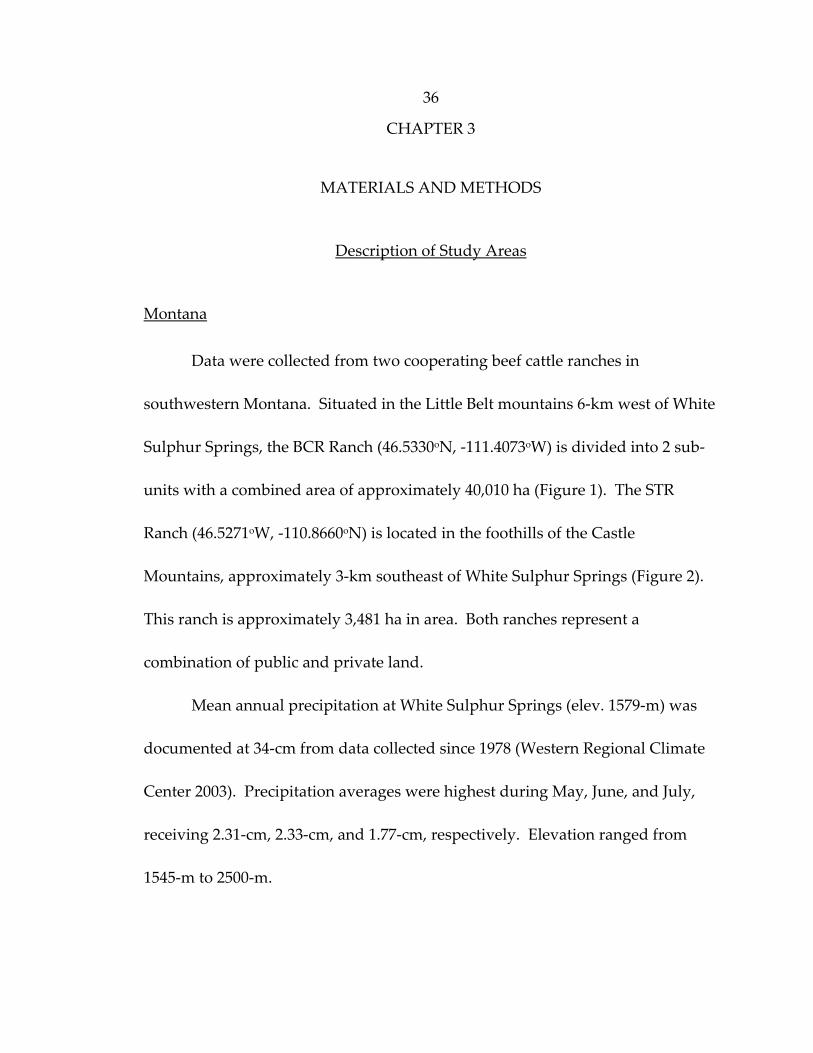
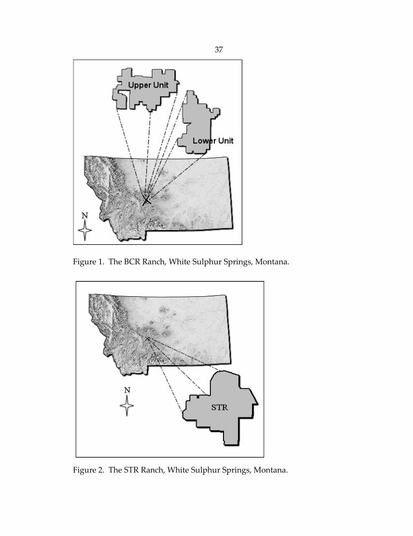
  Data were collected from two cooperating beef cattle ranches in 

southwestern Montana.  Situated in the Little Belt mountains 6‐km west of White 

Sulphur Springs, the BCR Ranch (46.5330oN, ‐111.4073oW) is divided into 2 sub‐

units with a combined area of approximately 40,010 ha (Figure 1).  The STR 

Ranch (46.5271oW, ‐110.8660oN) is located in the foothills of the Castle 

Mountains, approximately 3‐km southeast of White Sulphur Springs (Figure 2).  

This ranch is approximately 3,481 ha in area.  Both ranches represent a 

combination of public and private land. 

Mean annual precipitation at White Sulphur Springs (elev. 1579‐m) was 

documented at 34‐cm from data collected since 1978 (Western Regional Climate 

Center 2003).  Precipitation averages were highest during May, June, and July, 

receiving 2.31‐cm, 2.33‐cm, and 1.77‐cm, respectively.  Elevation ranged from 

1545‐m to 2500‐m. 

 

 

37 

 

Figure 1.  The BCR Ranch, White Sulphur Springs, Montana. 

 

 

 

 

 

 

 

 

 Figure 2.  The STR Ranch, White Sulphur Springs, Montana. 

 

38 Argiborolls‐lithic soils dominate the study areaʹs semiarid rangeland.  

Cryochrept soils are found extensively on mountain slopes in forested 

rangelands.  To a much lesser extent, loamy Haploborolls are found on glacial till 

plains, outwash terraces, sedimentary bedrock plains, and foothills (Montagne et 

al. 1982). 

Plant communities on these ranches included lowland sagebrush 

communities, mountain grasslands, and coniferous forests.  Coniferous forests 

are primarily dominated by Douglas fir (Pseudotsuga menziesii (Mirbel) Franco).  

Dominant perennial graminoids include Columbia needlegrass (Stipa nelsonii 

Scribner), needleandthread (Stipa comata Trin. & Rupr.), Idaho fescue (Festuca 

idahoensis Elmer), western wheatgrass (Pascopyrum smithii (Rydberg) Love), and 

bluebunch wheatgrass (Pseudoroegneria spicata (Pursh) Love). 

Common deciduous trees found in riparian areas are quaking aspen 

(Populus tremuloides Michaux) and black cottonwood (Populus trichocarpa Torr. & 

A.Gray).  Associated riparian shrub species include willow (Salix spp. L.), 

serviceberry (Amelanchier alnifolia Nutt.), and alder (Alnus spp. L.).  Sedges (Carex 

spp. L.) are common in the riparian areas. 

 

 

 

39 Sagebrush communities on the ranches are dominated by mountain big 

sagebrush (Artemisia tridentata vaseyana (Rydb.) Bovin) and Wyoming big 

sagebrush (Artemisia tridentata wyomingensis Nutt.) 

Wyoming 

  Data were also collected from two cooperating beef cattle ranches in 

northwestern Wyoming.  The MC Ranch (44.6101oN, ‐109.3877oW) is located  

20‐km west of Cody, Wyoming (Figure 3).  This ranch is approximately 21,294 ha 

in area.  The TE Ranch (44.2812oN, ‐109.4898oW) is located approximately 50‐km 

southwest of Cody, Wyoming.  This ranch is approximately 23,082 ha in area 

(Figure 3).   

  

 

 

 

 

 

   Figure 3.  The TE and MC Ranches of northwestern Wyoming. 

 

40 Mean annual precipitation in Cody, Wyoming (elev. 1521‐m) is 25‐cm 

based on precipitation data collected since 1925 (Western Regional Climate 

Center 2003).  This area received higher precipitation levels during May, June, 

and July, with averages of 1.63, 1.65, and 1.07‐cm, respectively.  Elevations range 

from 1650 to 3500‐m.  Topography is highly variable on these ranches, and range 

from glacial outwashes and rolling hills to steep, rocky outcrops.  Coarse Upland, 

Loamy, or Clayey range sites comprised the majority of landscapes in the 

sagebrush/mixed grass communities (SCS 1988). 

Plant communities at my study sites were dominated by mountain big 

sagebrush and Wyoming big sagebrush.  Prominent graminoids on the ranches 

included bluebunch wheatgrass, Columbia needlegrass, Idaho fescue, Indian 

ricegrass (Oryzopsis hymenoides Roem. And Schult.), needleandthread, plains 

reedgrass (Calamagrostis montanensis  Scribn), prairie june grass (Koeleria cristata  

L.), Sandberg bluegrass (Poa secunda Presl), spikefescue (Leucopoa kingii S. Wats) 

and western wheatgrass.   

        

 

41 

Elk and Cattle Locations 

Elk location data were collected by season.  For this study, December, 

January, and February were classified as winter months.  Spring months 

consisted of March, April, and May. The summer months were June, July, and 

August.  Fall months were September, October, and November.  Months were 

grouped into seasons based on seasonal changes in habitat use noted by Boyce 

(1991).  Elk activities during seasonal habitat use are assumed to be:  (1) winter 

survival; (2) spring movement and calving; (3) summer forage; and (4) fall 

breeding and post‐breeding (Roloff 1998, Roloff et al. 2001).  These seasonal 

designations corresponded well to seasonal changes in plant phenology. 

Elk group locations were collected on three ranches for all four seasons.  

On the BCR Ranch in Montana, elk locations were collected from May 2001 to 

November 2002.  In Wyoming, elk locations were collected on the TE and MC 

Ranches from November 2000 to November 2002.   

Cattle group locations were collected during the grazing season for all 

ranches.  I defined the grazing season as the period during spring through fall 

when beef cattle relied solely on rangelands with no supplemental hay offered.  

Even though cow groups were observed grazing during the winter feeding  

 

42 season, those locations were excluded because previously unobserved feeding 

bouts on haylines could subsequently influence feeding site selection in the 

pasture.  Grazing seasons were determined by individual ranch records and 

observations during flights.  To minimize the high variation of feeding site 

selection associated with age and physiology, only mature cows with calves were 

included in the data (Bell 1973, Bailey et al. 1996, Bailey 1999). 

Biweekly aerial surveys (26 flights/yr) in fixed‐wing aircraft were used to 

 detect and record elk and cattle locations.  Flights were scheduled the first and 

third week of every month.  Occasionally, inclement weather forced flights to be 

rescheduled, but monthly aerial observation periods were minimally one week 

apart to ensure independent elk and cattle locations. 

Observations were made by experienced pilots and observers.  Flights 

were conducted approximately 0.5 hours post sunrise which coincided with 

prime foraging time for elk and cattle (Craighead et al. 1973, Arnold and 

Dudzinski 1978, Green and Bear 1990).  At an altitude of 150‐m above the 

ground, aerial observations were conducted along 0.8‐km‐wide transects or, 

depending on the topography, followed contour lines and paralleled drainages.  

A complete census of the ranches was not consistently feasible throughout my  

 

 

43 study because of meteorological events associated with the rough, mountainous 

terrain.   

Cohesive animal group (e.g., at least 2 adults) locations were recorded 

using a global positioning system (GPS) receiver mounted inside the cockpit.  Elk 

and cattle groups were marked in non‐forested habitats because they were 

comparatively easier to observe than in forested habitats.  The GPS receiver 

recorded animal locations (e.g., waypoints) in the center of the group.  If animal 

groups were relatively large, more than one waypoint recorded the sub‐groups 

that formed the large animal groups.  Each recorded observation constituted one 

independent observation (Neu et al. 1974).  Single animals were excluded from 

our surveys based upon their higher variability in habitat selection (Sheehy and 

Vavra 1996, Bailey 1999).  Arha (1997) developed the elk HSI model for female 

elk and calves.  To be consistent, I rejected 100% bull elk groups and single cows 

with calves.  Hence, observations were collected on at least two adult cow elk in 

a group.   

 

 

44 

Model Inputs 

Land Cover Layer 

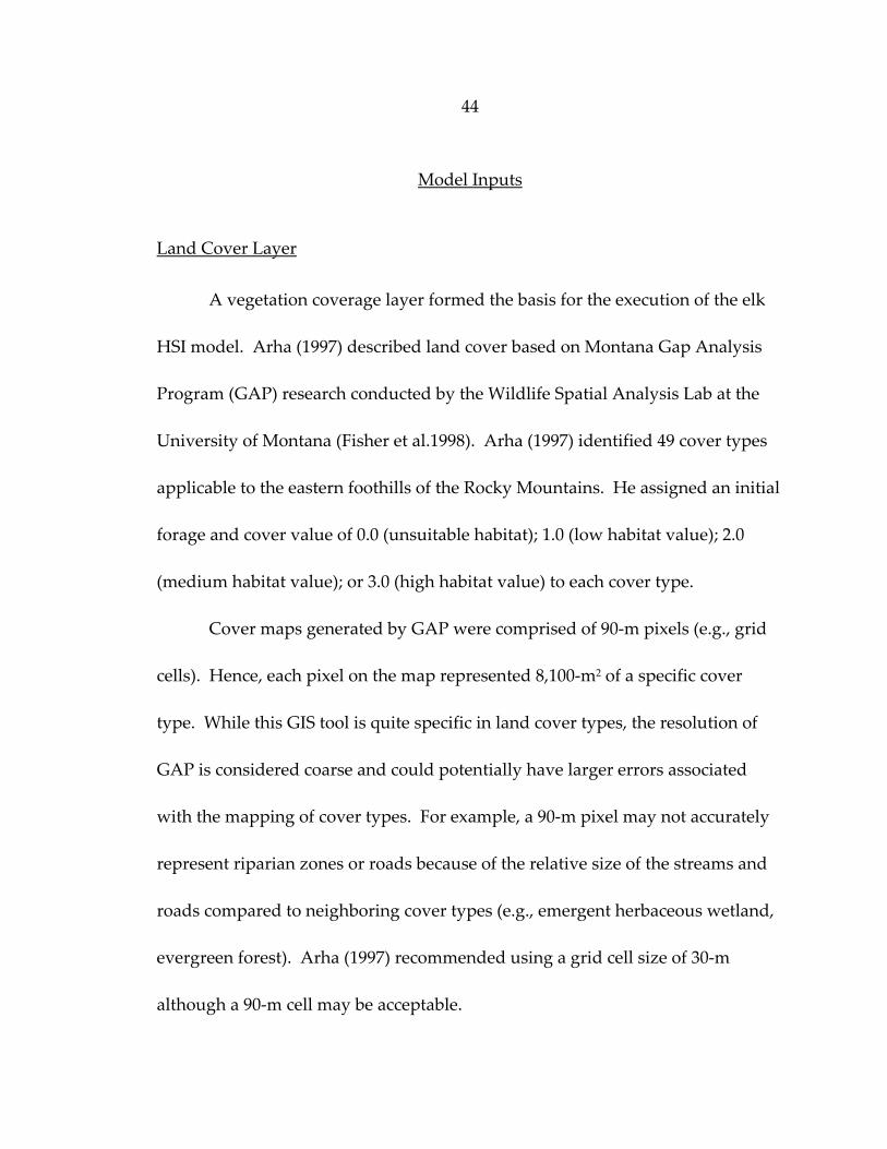
  A vegetation coverage layer formed the basis for the execution of the elk 

HSI model.  Arha (1997) described land cover based on Montana Gap Analysis 

Program (GAP) research conducted by the Wildlife Spatial Analysis Lab at the 

University of Montana (Fisher et al.1998).  Arha (1997) identified 49 cover types 

applicable to the eastern foothills of the Rocky Mountains.  He assigned an initial 

forage and cover value of 0.0 (unsuitable habitat); 1.0 (low habitat value); 2.0 

(medium habitat value); or 3.0 (high habitat value) to each cover type.   

Cover maps generated by GAP were comprised of 90‐m pixels (e.g., grid 

cells).  Hence, each pixel on the map represented 8,100‐m2 of a specific cover 

type.  While this GIS tool is quite specific in land cover types, the resolution of 

GAP is considered coarse and could potentially have larger errors associated 

with the mapping of cover types.  For example, a 90‐m pixel may not accurately 

represent riparian zones or roads because of the relative size of the streams and 

roads compared to neighboring cover types (e.g., emergent herbaceous wetland, 

evergreen forest).  Arha (1997) recommended using a grid cell size of 30‐m 

although a 90‐m cell may be acceptable.   

 

45   I used the Montana and Wyoming National Land Cover Dataset (NLCD) 

for the cover layers in the elk and cattle HSI models (NLCD 2001).  The NLCD 

was created from Landsat satellite TM imagery (circa 1992) and has a spatial 

resolution of 30‐m (i.e., one pixel equals an area of 900 square meters).  The 

NLCD has a 21‐class land cover classification scheme (Table 3, USGS  2001).  I 

used the NLCD because it was an up‐to‐date intermediate scale land cover data 

that would be continually updated to reflect ongoing changes in land cover use.   

For all four ranches, I obtained ʺshapefilesʺ of the ranch boundaries.  

Shapefiles were GIS files that defined the geometry and attributes of a 

geographically‐referenced feature.  By overlaying the ranch boundary shapefile 

with the Montana and Wyoming NLCD, I was able to demarcate cover categories 

found on the ranches.  To be consistent with Arha (1997), corresponding forage 

values used for the GAP layer were assigned to the NLCD cover types (Table 4). 

 

 

 

36 Table 3.  National Land Cover Data:  Land cover class descriptions (USGS 2001).  

 

 

 

 

 

 

 

 

 

46 

Code Cover Class Description11 Open Water All areas of open water, generally with less than 25% cover of vegetation/land cover.12 Perennial Ice/Snow All areas characterized by year‐long surface  cover of ice  and/or snow.21 Low Intensity Res. Includes areas with a  mixture  of constructed materials (30‐80% cover) and vegetation (20‐70% cover).22 High Intensity Res. Includes highly developed areas of constructed materials (80‐100% cover) and vegetation (<20% cover).23 Comm./Industrial/Trans. Includes infrastructure  (e.g., roads, railroads, etc.) and areas not classified as High Intensity Residential.31 Bare  Rock/Sand/Clay Perennially barren areas of bedrock, scarps, talus, and other accumulations of earthen material.32 Quarries/Strip Mines Areas of extractive  mining activities with significant surface  expression.33 Transitional Areas of sparse  veg. cover (< 25 %) that are  dynamically changing from one  land cover to another.41 Deciduous Forest Areas dominated by trees where  75% of the  tree  spp. shed foliage  due  to seasonal change.42 Evergreen Forest Areas dominated by trees where  75%  of the  tree  species maintain their leaves all year.43 Mixed Forest Areas with trees that neither deciduous nor evergreen spp. represent more  than 75 % of cover present.51 Shrublands Areas dominated by shrubs; shrub canopy accounts for 25‐100 % of the  cover.61 Orchard/Vineyards/Other Areas planted or maintained for the  production of fruits, nuts, berries, or ornamentals.71 Grasslands/Herbaceous Areas dominated by upland grasses and forbs and usually not subjected to intensive  management.  81 Pasture/Hay Areas of grasses and/or legumes planted for livestock grazing or for the  production of seed or hay crops.82 Row Crops Areas used for the  production of crops, such as corn, soybeans, vegetables, tobacco, and cotton.83 Small Grains Areas used for the  production of graminoid crops such as wheat, barley, oats, and rice.84 Fallow Areas used for alternation between cropping and tillage  and usually does not exhibit visible  vegetation.85 Urban/Recreational Grasses Vegetation (primarily grasses) planted in developed settings for recreation, erosion control, etc.91 Woody Wetlands Forest or shrubland vegetation accounts for 25‐100 % of the  cover where  soil is periodically saturated.92 Emergent Herb. Wetlands Herbaceous cover accounts for 75‐100 % of the  cover where  soil is periodically saturated.

 

 

 

47 Table 4.  Corresponding forage values assigned to NLCD. 

Winter Spring Summer Fall51   Shrubland 2 2 1 271   Grasslands/Herbaceous 3 3 3 381   Pasture/Hay 3 3 3 382   Row Crops 3 3 3 383   Small Grains 3 3 3 392   Emergent Herbaceous Wetlands 3 3 3 3

Forage ValuesCode NLCD Cover Class

  

Digital Elevation Models 

Digital elevation models (DEM) from Montana and Wyoming were used 

to obtain georeferenced data on aspect, elevation, and slope.  I acquired the 

Montana DEM from the Natural Resource Information System (NRIS) and the 

Wyoming DEM from the Wyoming Geographic Information Science Center 

(WyGISC) (Natural Resource Information Systems 2001, Wyoming Geographic 

Information Science Center 2001). 

Aspect and elevation were topographic attributes addressed in the winter, 

spring and fall elk HSI models (Arha 1997).  Elevation was not incorporated into 

the summer model because elevation was not considered a habitat hindrance 

(Arha 1997).  Additionally, Arha (1997) excluded aspect for the summer model 

stating there was no significant evidence of selection for one exposure over 

another.  Slope data were also obtained from the Montana and Wyoming DEM  

 

 

48 for the elk and cattle HSI models.  All topographic model variables for the elk 

and cattle models were produced on individual GIS layers for each ranch. 

Digital Raster Graphics 

A digital raster graphic (DRG) is a scanned image of a U.S. Geological 

Survey (USGS) standard series topographic map georeferenced to the surface of 

the earth and fit to the Universal Transverse Mercator projection (USGS 2003).  

Montana DRG were obtained from the Montana State Library (Natural Resource 

Information System 2001).  Wyoming DRG were obtained from the Wyoming 

Geographic Information Advisory Council (2001).  The scale of all DRG was 

1:24,000. 

Streams, lakes, ponds, springs and all naturally occurring perennial water 

sources found within the ranch boundaries on the DRG were digitized using 

ArcView 3.3 (ESRI 2002).  Digitizing converted the positions of these features on 

the DRG to a series of x, y coordinates.  These coordinates were later used for 

spatial analysis (e.g., determining distance from water).  Additionally, all ranch 

managers were consulted to determine the locations of stock tanks and 

developed water sites generally not found on the DRG.  These sites were also 

digitized and combined with the other water data in order to have a more 

accurate representation of available water sources.  Consequently, a water layer  

 

49 was produced for each ranch that was used for spatial analysis in the cattle 

model. 

Human disturbance represented by state highways, county roads, ranch 

roads and trails were digitized for the elk model.  I obtained ranch road locations 

from all four ranch managers.  All road types were digitized inside the ranch 

boundaries.  Additionally, I digitized all road types outside the ranch boundaries 

up to the maximum distance for a given road class as described by Arha (1997).  

Hence, the value of a pixel located inside the ranch boundary and in close 

proximity to the ranch perimeter was determined by pixels representing road 

classes outside the ranch boundary.  Trails were only used in the fall elk model 

because of increased use by humans during the hunting season. 

Model Application 

Elk Model 

Arha (1997) described forage and cover components in the elk model in 

order to derive the final elk HSI value (Figure 4).  In order to detect elk feeding 

site selection, I modified the existing elk model by excluding the cover 

component.  Cover was not entirely dismissed, however, as Arha (1997) included 

a distance from cover variable in the forage component of the elk model.   

 

50 

Initial Forage Value  Initial Cover Value 

Elevation  Elevation 

Aspect Modified

Cover Modified Cover Modified 

Disturbance 

Final CV Final FV  

Forage Component Cover Component 

Final Elk HSI = max(FV, 

 

 

 

 

 

 

 

 

 

 

 

 

Figure 4.  Conceptual elk HSI Model (Arha 1997).  

To determine availability, the forage component was further modified so 

that only non‐forested cover types were used in the model.  Thus, I excluded 

evergreen and deciduous forests, water, bare rock, and quarries from the NLCD 

cover layer.  This modified cover layer illustrated a more representative form of 

availability for elk feeding sites in non‐forested cover types (Table 5). 

 

 

51 Table 5.  Available elk habitat modified by excluding forested habitats.   

Ranch Total Area (ha) Adjusted Area (ha)BCR 40,010 31,888MC 21,294 11,450TE 23,082 16,298  

 For each ranch, the layers comprised of the NLCD, elevation, aspect, 

distance to cover and roads were assigned values to reflect their potential 

suitability for elk selection (Arha 1997).  Values of these variables potentially 

changed or were excluded in specific seasonal models as described by Arha 

(1997, Appendix A). 

Final elk habitat suitability coverages were mapped in ARC/INFO GRID 

format using ARC/INFO Macro Language (AML) programs that incorporated 

the model inputs for each of the seasons (Arha 1997).  After the models were run, 

each 30‐m pixel had a final suitability score assigned to it:  high habitat suitability 

(3.0); medium habitat suitability (2.0); low habitat suitability (1.0); and unsuitable 

habitat (0.0).  Final habitat suitability maps were comprised of a matrix of grids 

(e.g., pixels) that became aggregated into relatively contiguous, homogeneous 

units (e.g., patches).  Thus, each patch was composed of many grid cells.  By 

using GIS analysis, suitability value classes were generated for all patches.   

    

 

52 

Cattle Model 

Holechek (1988) developed a beef cattle stocking rate model that 

integrated total usable forage, forage demand, calculation of stocking rate and 

adjustment of the stocking rate for distance from water and percent slope.  To 

predict cattle feeding site selection, I modified this stocking rate cattle model and 

integrated a non‐forested NLCD cover layer with adjustments for percent slope 

and distance from water.  All non‐forested cover types were assigned an initial 

forage value of 3.0 (i.e., optimal suitability) because I assumed these cover types 

had high forage value for cattle.  An ARC/INFO AML was created for this cattle 

selection model (Appendix B ).   

In order to integrate the NLCD cover layer with slope, the initial forage 

value (e.g., 3.0) was multiplied by a multiplier value associated with the slope 

value (Table 6).  At this point, the cell had a value of either 3, 2.1, 1.2 or 0.  To 

integrate distance from water with the combined layers of cover and slope, I 

multiplied the current cell value with the multiplier associated with distance 

from water (Table 7).  At this point, the cell had a value of 3 , 2.1, 1.5, 1.2, 1.05, 0.6 

or 0.  These values were then rounded to the nearest integer value of 3, 2, 1 or 0 

to produce the final habitat suitability scores.   

 

 

53  Table 6.  Percent slopes and associated multiplier values. 

Slope (%) Initial Forage Value (IFV) Multiplier Value (MV)Slope‐Adjusted Value 

(IFV*MV)0 ‐ 10 3 1.0 311 ‐ 30 3 0.7 2.131 ‐ 60 3 0.4 1.2> 60 3 0.0 0

  Table 7.  Integration of distance from water values with slope‐adjusted values to determine final adjusted values. Distance from Water 

(km)Multiplier Value 

(MV)Slope‐Adjusted Value 

(SAV)1Final Adjusted Value   FAV = (MV*SAV)2

0 ‐ 1.60 1.0 3.0, 2.1, 1.2, or 0.0 3.0, 2.1, 1.2, or 0.01.70 ‐ 3.22 0.5 3.0, 2.1, 1.2, or 0.0 1.5, 1.05, 0.6, or 0.0> 3.22 0.0 3.0, 2.1, 1.2, or 0.0 0

1 For each distance category, the SAV is a unique number derived from the slope‐adjusted   value.  Outcomes of potential cell values are presented.2 The FAV is a unique number.  Outcomes of potential cell values are presented.   

Elk are capable of traversing large tracts of land, and fences do not 

generally restrict elk movement.  Therefore, I assumed that all resources were 

available to elk on all ranches.  Conversely, cattle do not have access to all 

available areas on the ranches.  Fenced pastures and management decisions 

directly influence where cattle graze.  Hence, pastures were considered as unique 

units of availability.  Grazing records that documented gate closures between 

pastures helped to determine total availability.  If documentation did not exist, I 

assumed that the pasture with cattle present was the only resource unit available 

to them.  I also assumed that the ability to detect selection would occur in larger‐ 

 

54 sized pastures and in pastures where cattle grazed for a relatively longer time.  

These two criteria were not considered mutually exclusive.  Grazing records 

were examined to determine the length of time cattle were in pastures.  In order 

to detect selection, I only used pastures that grazed cattle for more than two 

weeks and were greater than 200 ha.   

Statistical Methods 

Sampling protocol A was used to detect evidence of resource selection 

(Manly et al. 1993).  Hence, animal locations, available units, and used units were 

randomly sampled across the ranches.  Individual animals were not identified in 

our study because sampling was conducted at the population level (Manly et al. 

1993).   

  Experimental units were the patches generated from the 30‐m grids (e.g., 

habitat suitability values).  Abiotic and biotic components of the elk and cattle 

models were not subject to change.  Thus seasonal elk locations were pooled 

across the years and cattle locations were combined across the years if locations 

occurred in the same pasture.  Chi‐squared analyses were used to determine 

whether there was a significant difference between the expected use of suitability 

classes and the observed frequency of use (Neu et al. 1974).  I used SAS 8.02  

 

55 (1996) to test the null hypothesis that animals used habitat in proportion to 

availability.  The level of significance was determined a priori at 0.05.   

  Manly et al. (1993) described two important assumptions for resource 

selection studies:  1) Animals have free and equal access to all available resource 

units; and 2) resource units are sampled randomly and independently.  The first 

assumption was satisfied because elk have a high degree of mobility and were 

capable of traversing the study sites without impediment.  Cattle also had access 

to all available resources because availability was defined by pastures.  The 

second assumption was also met because the sampling design was based upon 

surveying study sites at least one week apart to detect independent animal 

locations.   

Selection ratios were used to detect selection and avoidance by yielding 

values proportional to the probability of use of a resource unit (Manly et al. 

1993).  Selection functions were estimated using the following equation, where Si 

represents the selection ratio, Ui refers to the observed use and Pi refers to 

expected use.  If selection ratios equaled 1.0, use was said to be non‐selective. 

Si = Ui/Pi

 

 

 

56 Selection occurred when Si was greater than 1.0 .  Avoidance occurred when the 

Si value was less than 1.0.  Preference for specific habitat classes was determined 

by using Bonferroni confidence intervals (Neu et al. 1974, Manly et al. 1993).  

 

57 CHAPTER 4 

RESULTS 

NLCD Landcover Classes  

According to the NLCD, grasslands/herbaceous was the dominant cover 

class on the STR and BCR Ranches in Montana and on the MC and TE Ranches in 

Wyoming (Tables 8 and 9, respectively).  Because I was primarily interested in 

elk and cattle feeding sites, I removed non‐herbaceous cover classes to establish 

available herbaceous cover classes for potential feeding sites in Montana and 

Wyoming.   

Elk and Cattle Feeding Site Locations 

  A total of 1,076 independent elk group locations and 806 independent 

cattle group locations were collected during the course of my study.  Elk group 

locations were collected on one ranch in Montana and two ranches in Wyoming.  

During the winter, spring, summer, and fall seasons, 268, 452, 209, and 147 elk 

group locations were recorded, respectively.   

Cattle locations were collected in occupied pastures on two ranches in 

Montana and two ranches in Wyoming.  In Montana, 627 cattle group locations  

 

58 were collected in 18 pastures.  A combined total of 180 cattle group locations 

were collected in 10 pastures in Wyoming.   

 Table 8.  Total NLCD cover classes for the BCR and STR Ranches, Montana.   

Area (ha) Area (%) Area (ha) Area (%)Open Watera 358                  0.68 1                      0.02Commercial/Industrial/Transportationa n/a n/a 5                      0.14Bare Rock, Sand, and Claya 13                    0.03 0                      0.01Quarries/Strip Mines/Gravel Pitsa 4                      0.01 n/a n/aDeciduous Foresta 1,728               3.30 68                    1.74Coniferous Foresta 10,718        20.46 322              8.28Shrubland 3,385             6.46 262                 6.72Grasslands/Herbaceous 34,846           66.52 2,539              65.27Pasture/Hay 493                0.94 419                 10.76Row Crops 227                0.43 61                   1.56Small Grains 336                0.64 132                 3.40Fallowa 265                  0.51 82                    2.11Woody Wetlandsa 7                      0.01 n/a n/a

Total 52,381 100 3,890              100a Cover classes removed from the NLCD in the elk and cattle HSI models.

BCR Ranch STR RanchNLCD Cover Class

  

Elk Habitat Selection 

Four elk habitat suitability categories were tested using Chi‐squared 

goodness‐of‐fit tests to determine if elk exhibited selection among habitat 

suitability categories.  Selection ratios (S) determined selection, avoidance, or 

non‐selection by elk within a given habitat suitability category.   

   

 

59 Table 9.  Total NLCD cover classes for the MC and TE Ranches, Wyoming.   

Area (ha) Area (%) Area (ha) Area (%)Open Watera < 1 0.00 4                      0.02Perennial Ice/Snowa 5                      0.02 1                      0.00Low Intensity Residentiala < 1 0.00 1                      0.00Bare Rock, Sand, and Claya 77                    0.36 3                      0.01Deciduous Foresta 25                    0.12 47                    0.20Evergreen Foresta 6,856               32.20 6,775               29.35Mixed Foresta 2                      0.01 4                      0.02Shrubland 5,155             24.21 6,160               26.69Grasslands/Herbaceous 9,098             42.73 9,796               42.44Pasture/Hay 27                  0.13 213                  0.92Row Crops 30                  0.14 19                    0.08Small Grains 10                  0.04 23                    0.10Fallowa 7                      0.03 17                    0.07Woody Wetlandsa < 1 0.00 10                    0.04Emergent Herbaceous Wetlands  1                    0.01 11                    0.05

Total 21,293           100 23,084             100a Cover classes removed from the NLCD in the elk and cattle HSI models.

NLCD Cover ClassMC Ranch TE Ranch

 

Winter 

For illustrative purposes, Figure 5 depicts the distribution of winter elk 

group locations on the habitat suitability map for the upper unit of the BCR 

Ranch.  According to the winter elk model, only the TE Ranch contained areas 

categorized as unsuitable (Table 10).  Contrary to model expectations, elk 

significantly selected for the low suitability classes on the MC (S = 1.93) and TE 

ranches (S = 1.87) during the winter season.  Furthermore, elk avoided the  

  

 

60 medium suitability class on the MC Ranch (S = 0.53) and the high suitability class 

on the TE Ranch (S = 0.36).  On the BCR Ranch in Montana, elk use was in 

proportion to availability.  Hence, the null hypothesis could not be rejected.   

 Table 10.  Feeding site selection by elk in winter.   Habitat Suitability 

Class (Value)n

Observed (U)

Expected (P)

S (U/P)Lower Bound

Upper Bound

Low (1) 1 0.03 0.01 2.70 ‐3.68 9.08Medium (2) 14 0.38 0.44 0.86 0.43 1.29High (3) 22 0.59 0.55 1.08 0.73 1.43

Low (1) 22 0.58 0.30 1.93* 1.29 2.57Medium (2) 9 0.24 0.45 0.53* 0.16 0.89High (3) 7 0.18 0.25 0.74 0.13 1.34

Unsuitable (0) 2 0.01 0.01 1.04 ‐0.78 2.86Low (1) 72 0.38 0.20 1.87* 1.43 2.30Medium (2) 105 0.54 0.59 0.92 0.77 1.07 High (3) 14 0.07 0.20 0.36* 0.13 0.60

BCR Ranch, Montana:  X2 (df = 2) = 1.53    (p = 0.47)

MC Ranch, Wyoming:  X2 (df = 2) = 14.35    (p < 0.01)

TE Ranch, Wyoming:  X2 (df = 3) = 45.27    (p < 0.01)

* = Significantly different from 1.0 (p = 0.05)

 

 

 

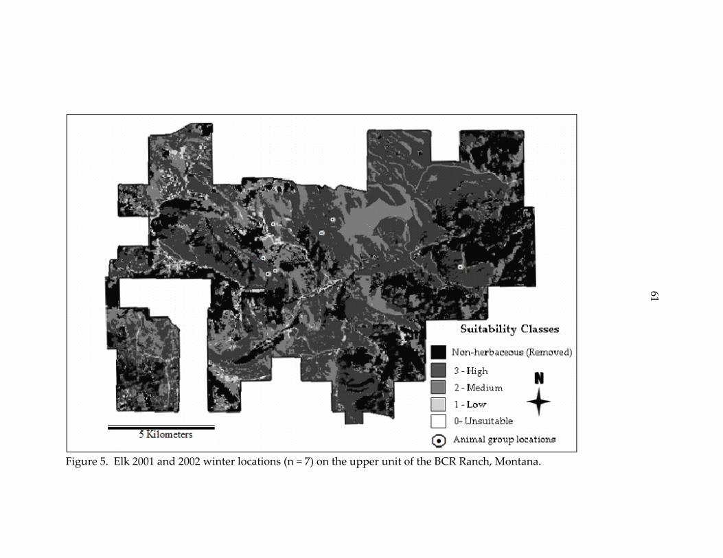
60

5 Kilometers 

                       

61 

 Figure 5.  Elk 2001 and 2002 winter locations (n = 7) on the upper unit of the BCR Ranch, Montana. 

 

62 

Spring 

  According to the spring elk model, all four suitability classes were 

represented on MC and TE Ranches in Wyoming (Table 11).  The BCR Ranch in 

Montana did not contain areas characterized as unsuitable spring habitat.  Elk 

avoided the low suitability classes on the MC Ranch (S = 0.49) and the BCR 

Ranch (S = 0.45).  Elk use on the TE Ranch in Wyoming was non‐selective.  The 

null hypothesis could not be rejected. 

 Table 11.  Feeding site selection by elk in spring. Habitat Suitability 

Class (Value)n

Observed (U)

Expected (P)

S (U/P)Lower Bound

Upper Bound

Low (1) 5 0.04 0.10 0.45* ‐0.02 0.91Medium (2) 51 0.46 0.36 1.27 0.95 1.58High (3) 56 0.50 0.54 0.93 0.72 1.14

Unsuitable (0) 2 0.03 0.01 2.82 ‐2.09 7.73Low (1) 7 0.10 0.20 0.49* 0.05 0.93Medium (2) 41 0.58 0.47 1.23 0.92 1.54High (3) 21 0.30 0.32 0.92 0.50 1.35

Unsuitable (0) 3 0.01 0.01 1.12 ‐0.48 2.72Low (1) 32 0.12 0.14 0.85 0.50 1.20Medium (2) 140 0.52 0.53 0.98 0.84 1.13High (3) 94 0.35 0.32 1.09 0.86 1.32

BCR Ranch, Montana:  X2 (df = 2) = 6.59    (p = 0.04)

* = Significantly different from 1.0 (p = 0.05)

MC Ranch, Wyoming:  X2 (df = 3) = 7.87    (p = 0.05)

TE Ranch, Wyoming:  X2 (df = 3) = 1.66    (p = 0.65)

  

 

63 

Summer 

  Elk selected (S = 1.29) high suitable habitat on the BCR Ranch but avoided 

the medium suitable habitat (S = 0.19) during the summer season (Table 12).  Elk 

use was in proportion to availability on the MC and TE Ranches in Wyoming, 

and the null hypothesis could not be rejected.   

 Table 12.  Feeding site selection by elk in summer.   Habitat Suitability 

Class (Value)n

Observed (U)

Expected (P)

S (U/P)Lower Bound

Upper Bound

Low (1) 19 0.15 0.20 0.77 0.38 1.15Medium (2) 4 0.03 0.17 0.19* ‐0.03 0.41High (3) 101 0.82 0.63 1.29* 1.16 1.43

Low (1) 20 0.41 0.40 1.02 0.63 1.41High (3) 29 0.59 0.60 0.99 0.72 1.25

Unsuitable (0) 2 0.06          0.11          0.51 ‐0.36 1.37Low (1) 10 0.28          0.36          0.77 0.25 1.29Medium (2) 2 0.06          0.07          0.79 ‐0.57 2.16High (3) 22 0.61          0.46          1.33 0.89 1.77

BCR Ranch, Montana:  X2 (df = 2) = 21.90    (p < 0.01)

* = Significantly different from 1.0 (p = 0.05)

MC Ranch, Wyoming:  X2 (df = 1) = 0.01  (p = 0.91)

TE Ranch, Wyoming:  X2 (df = 3) = 3.54  (p = 0.32)

 

Fall 

  Elk avoided the unsuitable class (S = 0.26) on the BCR Ranch and the low 

suitability class on the BCR Ranch (0.59) and the TE Ranch (S = 0.12) during the 

fall season (Table 13).  On the MC Ranch, elk also avoided the high suitable class  

 

64 (S = 0.14).  Elk selected for the medium suitability classes on the BCR (S = 2.51) 

and MC Ranch (S = 1.68).   

 Table 13.  Feeding site selection by elk in fall. 

Habitat Suitability Class (Value)

nObserved 

(U)Expected 

(P)S (U/P)

Lower Bound

Upper Bound

Unsuitable (0) 5 0.06 0.24 0.26* ‐0.02 0.53Low (1) 23 0.31 0.44 0.59* 0.32 0.85Medium (2) 47 0.48 0.20 2.51* 1.89 3.14High (3) 14 0.14 0.12 1.21 0.47 1.95

Low (1) 9 0.31 0.37 0.84 0.28 1.39Medium (2) 19 0.66 0.39 1.68* 1.14 2.22High (3) 1 0.03 0.24 0.14* ‐0.19 0.48

Unsuitable (0) 1 0.03 0.29 0.12* ‐0.17 0.41Low (1) 9 0.31 0.33 0.94 0.29 1.59Medium (2) 12 0.41 0.23 1.80 0.81 2.79High (3) 7 0.24 0.15 1.61 0.29 2.93

BCR Ranch, Montana:  X2 (df = 3) = 60.92    (p < 0.01)

MC Ranch, Wyoming:  X2 (df = 2) = 10.61  (p = 0.01)

TE Ranch, Wyoming:  X2 (df = 3) = 12.44  (p < 0.01)

* = Significantly different from 1.0 (p = 0.05)   

Cattle Habitat Selection 

BCR Ranch, Montana 

  A total of 270 cattle group locations were collected on five pastures 

located on the lower unit of the BCR Ranch (Table 14).  Cattle group locations  

 

 

65 were obtained during the 2001 and 2002 grazing seasons on Pastures 1, 2, 4, and 

5.  During the 2001 grazing season, cattle group locations were collected on 

Pasture 3.  For illustrative purposes, Figure 6 depicts a map of cattle habitat 

suitability, spatial arrangement of pastures, and associated cattle group locations.   

 Table 14.  Cattle study area on the lower unit pastures of the BCR Ranch, Montana.   

Pasture Number

Area (ha)* # Cattle Group Locations

1 2,493 1262 1,901 493 1,454 434 663 445 265 10

Total 6,776 272*Excluding forested and non‐herbaceous cover types.   

Table 15 summarizes the results of the cattle HSI model for the lower unit 

pastures of the BCR Ranch.  Approximately 10 percent of Pasture 5 was 

comprised of the high suitable habitat, but this category did not contain any 

cattle group locations and was consequently omitted from the Chi‐squared 

analysis.  Contrary to model expectations, cattle avoided the high suitability 

classes in Pasture 1 (S = 0.88) and Pasture 4 (S = 0.33) on the lower unit of the BCR 

Ranch.  There was no evidence of selection or avoidance in Pastures 2, 3, or 5. 

 

              66         

5 Kilometers   Figure 6.  BCR Ranch, Montana:  Cattle habitat suitability map of the lower unit pastures with cattle locations.  

67 Table 15.  Feeding site selection by cattle on the lower unit of the BCR Ranch, Montana.   

Low (1) 6 0.05 0.01 4.76 0.22 9.30Medium (2) 28 0.22 0.16 1.39 0.83 1.94High (3) 92 0.73 0.83 0.88* 0.77 0.99

Low (1) 1 0.02 0.02 1.06 ‐1.46 3.59Medium (2) 16 0.34 0.32 1.06 0.55 1.58High (3) 30 0.64 0.66 0.97 0.71 1.22

Low (1) 3 0.07 0.05 1.40 ‐0.47 3.26Medium (2) 17 0.40 0.43 0.92 0.50 1.33High (3) 23 0.53 0.52 1.03 0.68 1.38

Low (1) 11 0.25 0.15 1.67 0.62 2.71Medium (2) 31 0.70 0.71 0.99 0.76 1.22High (3) 2 0.05 0.14 0.33* ‐0.21 0.86

Low (1) 5 0.50 0.31 1.61 0.47 2.76Medium (2) 5 0.50 0.69 0.72 0.21 1.24* = Significantly different from 1.0 (p = 0.05)

Pasture 1:  X2(df = 2) = 22.39  (p < 0.01)

Pasture 2:  X2(df = 2) = 0.10  (p = 0.95)

Pasture 3:  X2(df = 2) = 0.47 (p = 0.79)

Pasture 4:  X2(df = 2) = 5.74 (p = 0.06)

S          (U/P)

Lower Bound

Upper Bound

Pasture 5:  X2(df = 1) = 1.69 (p = 0.19)

Habitat Suitability Classes (Values)

nObserved 

(U)Expected 

(P)

    Cattle group locations (n = 330) were collected on nine pastures located on 

the upper unit of the BCR Ranch in Montana (Table 16).  For illustrative 

purposes, Figure 7 shows the upper unit pasture with corresponding numbered 

pastures used for cattle habitat selection analysis.   

   

 

68 Table 16.  Cattle study area on the upper unit of the BCR Ranch, Montana.   Pasture Number

Area* (ha) # Cattle Group Locations

1 679 362 1,441 933 1,576 704 1,526 585 415 156 1,464 167 1,618 208 860 89 754 14

Total 10,333 330*Excluding forested and non‐herbaceous cover types.   

5 Kilometers 

Fig 

loc

col

  

 

 ure 7.  BCR Ranch, Montana:  Map of the upper unit pastures. 

During the 2001 and 2002 grazing seasons, I analyzed cattle group 

ations on Pastures 1, 2, 3, 4, 6, 8, and 9 (Table 17).  Cattle group locations were 

lected in Pasture 5 during the 2002 grazing season.   

69 Table 17.  Feeding site selection by cattle on the upper unit of the BCR Ranch, Montana. 

Low (1) 10 0.28 0.17 1.63 0.65 2.62Medium (2) 26 0.72 0.83 0.87 0.67 1.07

Low (1) 25 0.27 0.26 1.03 0.61 1.46Medium (2) 57 0.61 0.65 0.94 0.76 1.13High (3) 11 0.12 0.09 1.31 0.42 2.21

Low (1) 35 0.50 0.53 0.94 0.67 1.21Medium (2) 25 0.36 0.40 0.89 0.55 1.24High (3) 10 0.14 0.07 2.04 0.61 3.47

Low (1) 28 0.48 0.42 1.15 0.78 1.52Medium (2) 28 0.48 0.50 0.97 0.65 1.28High (3) 2 0.03 0.08 0.43 ‐0.29 1.15

Unsuitable (0) 2 0.13 0.18 0.74 ‐0.43 1.91Low (1) 6 0.40 0.45 0.89 0.22 1.56Medium (2) 7 0.47 0.37 1.26 0.43 2.10

Low (1) 5 0.31 0.28 1.12 0.12 2.11Medium (2) 8 0.50 0.58 0.86 0.35 1.38High (3) 3 0.19 0.14 1.34 ‐0.33 3.01

Low (1) 1 0.05 0.10 0.50 ‐0.67 1.67Medium (2) 10 0.50 0.45 1.11 0.52 1.71High (3) 9 0.45 0.45 1.00 0.41 1.59

Pasture 7:  X2(df = 2) = 0.61 (p = 0.74)

Pasture 6:  X2(df = 2) = 0.49 (p = 0.78)

Pasture 1:  X2(df = 1) = 2.96  (p = 0.09)

Pasture 2:  X2(df = 2) = 1.05  (p = 0.59)

Pasture 3:  X2(df = 2) = 5.75  (p = 0.06)

Pasture 4:  X2(df = 2) = 2.05 (p = 0.35)

S          (U/P)

Lower Bound

Upper Bound

Pasture 5:  X2(df = 2) = 0.64 (p = 0.72)

Habitat Suitability Classes (Values)

nObserved 

(U)Expected 

(P)

  

 

 

70 Table 17.  (contʹd).  Feeding site selection by cattle on the upper unit of the BCR Ranch, Montana. 

Medium (2) 3 0.38 0.53 0.71 ‐0.02 1.43High (3) 5 0.63 0.47 1.33 0.51 2.15

Medium (2) 7 0.50 0.50 1.00 0.40 1.60High (3) 7 0.50 0.50 1.00 0.40 1.60

Pasture 9:  X2(df = 1) = 0.00 (p = 1.00)

S          (U/P)

Lower Bound

Upper Bound

Habitat Suitability Classes (Values)

nObserved 

(U)Expected 

(P)

Pasture 8:  X2(df = 1) = 0.77 (p = 0.38)

  Pasture 7 contained cattle group locations that were collected during the 2001 

grazing season.  According to the model, 10 percent of Pasture 1 was classified as 

high suitable habitat, but no cattle group locations were observed in this area.  

The model also classified low suitable habitat in Pastures 8 and 9 (10 and 2 

percent, respectively) but no cattle groups were observed in this category.  

Consequently, these categories were omitted from Chi‐squared analyses.  I did 

not detect evidence of selection or avoidance for any suitability class in the upper 

unit pastures of the BCR ranch.   

STR Ranch, Montana 

  A total of 27 cattle group locations were collected on four pastures located 

on the STR Ranch (Table 18).  Cattle group locations were collected in Pasture 1 

during the 2002 grazing season and in Pasture 2 for 2001.  For Pastures 3 and 4, 

cattle group locations were collected during the 2001 and 2002 grazing seasons.   

 

71 Figure 8 illustrates spatial distribution of pastures used for habitat selection 

analyses.   

 Table 18.  Cattle study area on the STR Ranch, Montana.   

Pasture     Number Area* (ha) # Cattle Group Locations

1 224 92 175 43 198 64 239 8

Total 836 27*Excluding forested and non‐herbaceous cover types.    

  

2 km 3 Kilometers 

Figure 8.  Pasture locations: STR Ranch, Montana.    

 

 

72 Cattle use was in proportion to availability in all four pastures (Table 19).  

Hence, cattle use was non‐selective in these pastures and the null hypothesis 

could not be rejected.   

 Table 19.  Feeding site selection by cattle on the STR Ranch, Montana. 

Medium (2) 6 0.67 0.54 1.24 0.59 1.89High (3) 3 0.33 0.46 0.72 ‐0.05 1.48

Low (1) 1 0.25 0.46 0.54 ‐0.51 1.60High (3) 3 0.75 0.54 1.39 0.49 2.29

Low (1) 1 0.17 0.10 1.67 ‐1.74 5.08Medium (2) 5 0.83 0.90 0.93 0.55 1.30

Medium (2) 1 0.12 0.05 2.50 ‐2.74 7.74High (3) 7 0.88 0.95 0.92 0.65 1.20

S          (U/P)

Lower Bound

Upper Bound

Habitat Suitability Classes (Values)

nObserved 

(U)Expected 

(P)

Pasture 1:  X2(df = 1) = 0.58  (p > 0.46)

Pasture 2:  X2(df = 1) = 0.71  (p = 0.40)

Pasture 3:  X2(df = 1) = 0.30  (p = 0.59)

Pasture 4:  X2 (df = 1) = 0.95  (p = 0.33)

  

MC Ranch, Wyoming 

  During the 2001 and 2002 grazing seasons, 56 cattle group locations were 

collected on 5 pastures on the MC Ranch (Table 20).  Figure 9 illustrates spatial 

arrangements of pastures used for selection analyses.   

    

 

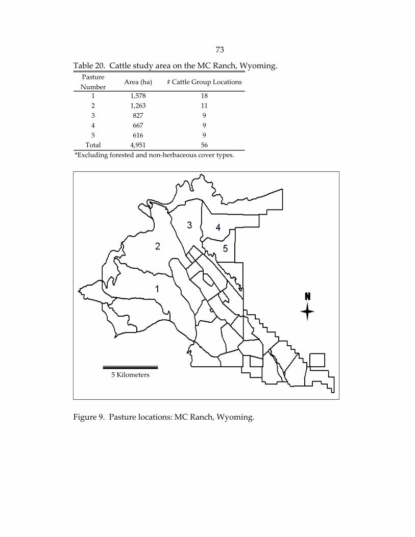
73 Table 20.  Cattle study area on the MC Ranch, Wyoming. 

Pasture Number

Area (ha) # Cattle Group Locations

1 1,578 182 1,263 113 827 94 667 95 616 9

Total 4,951 56*Excluding forested and non‐herbaceous cover types.   

 5 km 

 5 Kilometers 

Figure 9.  Pasture locations: MC Ranch, Wyoming. 

 

    

 

74 Only Pasture 1 contained the entire array of suitability categories (Table 

21).  Cattle use was proportionate to availability in Pastures 2, 3, 4 and 5.  In 

Pasture 1, cattle avoided the low suitability class (S = 0.42).   

 Table 21.  Feeding site selection by cattle on the MC Ranch, Wyoming. 

Unsuitable (0) 1 0.06 0.07 0.79 ‐1.13 2.72Low (1) 3 0.17 0.40 0.42* ‐0.13 0.97Medium (2) 13 0.72 0.49 1.47 0.94 2.01High (3) 1 0.06 0.04 1.39 ‐1.98 4.76

Low (1) 6 0.55 0.57 0.96 0.37 1.55Medium (2) 5 0.45 0.43 1.06 0.27 1.84

Medium (2) 7 0.78 0.81 0.96 0.58 1.34High (3) 2 0.22 0.19 1.17 ‐0.46 2.80

Medium (2) 5 0.56 0.54 1.03 0.34 1.72High (3) 4 0.44 0.46 0.97 0.16 1.77

Medium (2) 5 0.50 0.68 0.74 0.02 1.45High (3) 4 0.33 0.07 4.76 ‐1.82 11.35

S (U/P)Lower Bound

Upper Bound

Habitat Suitability Classes (Values)

nObserved 

(U)Expected 

(P)

Pasture 5:  X2(df = 1) = 0.0088  (p = 0.93)

* = Significantly different from 1.0 (p = 0.05)

Pasture 1:  X2(df = 3) = 4.59  (p = 0.20)

Pasture 2:  X2(df = 1) = 0.03  (p = 0.87)

Pasture 3:  X2(df = 1) = 0.06  (p = 0.13)

Pasture 4:  X2(df = 1) = 0.01  (p = 0.93)

 

TE Ranch, Wyoming 

  Cattle group locations on 5 (n = 124) were collected on 5 pastures on the 

TE Ranch (Table 22).  Figure 10 illustrates spatial arrangements of pastures used  

 

 

75 for selection analyses.  Cattle group locations were collected during the 2001 and 

2002 grazing seasons on Pastures 1, 4, and 5.  During the 2001 grazing season, 

cattle group locations were collected on Pasture 3.  Cattle locations were obtained 

during the 2002 grazing season on Pasture 2.   

 Table 22.  Cattle study area on the TE Ranch, Wyoming. Pasture Number

Area* (ha) # Cattle Group Locations 

1 2,455 642 737 53 609 74 722 115 2,557 37

Total 7,080 124*Excluding forested and non‐herbaceous cover types.     Cattle used habitat suitability classes in Pasture 5 disproportionately to 

availability (Table 23).  Cattle selected the medium suitability class (S = 1.45) and 

avoided the low suitability class (0.21).  Cattle used habitat suitability classes in 

Pastures 1, 2, 3, and 4 in proportion to availability.   

 

 

 

     

 

76                        5 Kilometers    

Figure 10.  Pasture locations:  TE Ranch, Wyoming.             

 

77 Table 23.  Feeding site selection by cattle on the TE Ranch, Wyoming. 

Low (1) 26 0.41 0.43 0.94 0.60 1.29Medium (2) 35 0.55 0.49 1.12 0.81 1.42High (3) 3 0.05 0.08 0.59 ‐0.21 1.38

Low (1) 1 0.20 0.42 0.48 ‐0.48 1.43Medium (2) 4 0.80 0.58 1.38 0.69 2.07

Medium (2) 3 0.43 0.69 0.62 0.01 1.23High (3) 4 0.57 0.31 1.84 0.49 3.19

Medium (2) 7 0.64 0.70 0.91 0.45 1.37High (3) 4 0.36 0.30 1.21 0.13 2.29

Low (1) 3 0.08 0.38 0.21* ‐0.07 0.50Medium (2) 29 0.78 0.54 1.45* 1.15 1.75High (3) 5 0.14 0.08 1.69 0.01 3.37

S          (U/P)

Lower Bound

Upper Bound

Habitat Suitability Classes (Values)

nObserved 

(U)Expected 

(P)

Pasture 1:  X2(df = 2) = 0.21  (p = 0.50)

Pasture 2:  X2(df = 1) = 0.99  (p = 0.32)

Pasture 3:  X2(df = 1) = 2.24  (p = 0.13)

Pasture 4:  X2(df = 1) = 0.21  (p = 0.65)

Pasture 5:  X2(df = 2) = 14.18  (p < 0.01)

* = Significantly different from 1.0 (p = 0.05)  

 

78 CHAPTER 5 

 

DISCUSSION 

I evaluated the GIS‐based modified elk and cattle HSI models developed 

by Arha (1997) and Holechek (1988), respectively,  on four beef cattle ranches in 

Montana and Wyoming.  The objective of my research was to test the hypothesis 

that elk and cattle feeding site selection were positively related to HSI categories.  

I predicted that elk and cattle would avoid the unsuitable class (e.g., HSI = 0) but 

incrementally increase selection of the higher suitability classes (HSI = 1.0, 2.0, 

and 3.0).  If the models accurately predicted elk and cattle use, I could endorse 

the use of these models as reliable resource management tools. 

Relatively few studies are directly comparable to this study.  I know of no 

other study that tested a seasonal elk HSI model or a cattle HSI model at a 

similar landscape scale using independent data.  Based on the available 

literature, multiple regression appears to be widely used to develop habitat 

suitability models (Thomas et al. 1979, Lonner 1984, Grover and Thompson 

1986).  However, many of these models are constructed and tested with the same 

data (Brooks 1997).  These HSI models may perform well at the locations where 

the data used to construct them were collected, but the accuracy may be low on 

other geographical locations.   

 

79 The models used in this study were constructed from knowledge 

synthesized from previous research on elk and cattle habitat selection.  Holechek 

(1988) and Arha (1997) assigned values to habitat variables that were integrated 

as the models derived HSI categories.  The associations of animal observations 

and HSI values were evaluated using Chi‐squared tests.  Thus, I could not 

determine which specific habitat variables (e.g., elevation, slope, aspect, 

vegetative cover, distance from water, distance from roads) significantly 

contributed to elk and cattle habitat selection.   

Seasonal Habitat Selection and Use by Elk 

Winter 

  The winter model performed contrary to what I expected.  Elk selected the 

low suitability class on the MC and TE Ranches in Wyoming but avoided the 

high suitability areas on the TE Ranch.  Elk may have avoided high suitability 

areas and selected for low suitability areas because the HSI model did not 

account for foraging areas found in forested areas or because of complex social 

and biological interactions.  

I was unable to detect selective use or avoidance of any suitability classes 

on the Montana ranch during winter.  Similarly, a winter elk HSI model used in  

 

 

80 west‐central Alberta, Canada, did not detect elk selection or avoidance for any 

suitability class (Jones 1997).   

  Arha (1997) did not include slope in the winter model, and this exclusion 

may contribute to some of the inconsistencies of the model during this season.  

According to Mackie (1970), approximately 65 percent of the elk studied used 

slopes of 0 to 18 percent during winter, an increase from 50 percent use during 

spring and autumn.  Conversely, McCorquodale (2003) determined that at a 

home range scale, female elk selectively used more areas of steep slopes (>50%) 

and moderately steep slopes (40‐49%) during winter.  At patch scales, cow elk 

preferred 30 – 39 percent slopes (McCorquodale 2003).   

Spring 

  The predictive ability of the spring elk model was poor.  Elk did not select 

for any suitability class on any of the ranches in Montana and Wyoming.  

However, elk avoided the low suitability class, but only on the MC Ranch in 

Wyoming.  Elk use was non‐selective over the remaining ranches and suitability 

classes.   

Other variables not addressed in the elk model may have helped to 

predict elk feeding site selection.  A study conducted by Grover and Thompson 

(1986) investigated factors that influenced elk spring feeding selection in  

 

81 southwestern Montana.  Based on regression  models, they concluded that 

previous cattle use influenced elk spring feeding site selection.  Research by 

Crane (2002) concluded that residual forage was the primary habitat attribute 

that influenced spring elk feeding site selection.  The elk model I tested did not 

incorporate a residual forage variable, however, this variable may be an essential 

model component. 

In addition, distance from the nearest visible road, density of bunchgrass 

plants, and distance from cover accounted for 65 percent of the variation in elk 

feeding distribution (Grover and Thompson 1986).  Crane (2002) also determined 

that distance from forested cover was a significant variable in elk resource 

selection functions.  Arha (1997) accounted for presence of roads but did not 

account for sightability of roads.  For example, elk may feel a sense of security in 

areas less than 20‐m from a ranch road if the topography shields the road from 

the elk’s view.  Hence, the suitability index value for distance from cover may be 

artificially low in some areas of the ranches.   

Summer 

  The summer suitability model did not consistently predict elk use across 

the three ranches.  On the BCR Ranch in Montana, elk selected for the high  

  

 

82 suitability level but avoided the medium suitability level.  The model also 

performed poorly on the Wyoming ranches.  My findings concur with the 

outcome of a summer elk model tested by Roloff et al. (2001).  Their elk model 

also did not consistently predict summer elk use.  The authors reported that elk 

used topographic barriers for cover during the summer months, but this feature 

was not incorporated into the model.   

  Arha (1997) did not incorporate aspect into the summer elk model because 

he assumed there was no significant evidence of selection by elk for one 

exposure over another.  In western Montana, Skovlin (1982) documented elk use 

on north‐facing slopes because of cooler temperatures in the summer.  Marcum 

(1975) noted that cow elk selected southwesterly through northwesterly and 

northeasterly exposures during the summer in Montana.  Based on these 

previous studies, aspect may be an important variable that could help predict 

summer elk habitat selection.   

According to the summer HSI model output, the MC Ranch contained all 

four levels of suitability.  However, elk were only located on the low and high 

suitability classes.  Because of the limitations of Chi‐squared analysis, I could not 

consider the unsuitable and medium suitability classes available to elk in my  

  

 

83 analyses, even though these classes were actually available to the elk on the 

ranch.   

Fall 

  Relative to the other seasonal models, the fall model was slightly better in 

predicting elk use on the BCR Ranch in Montana.  Elk selected for medium 

suitable habitat on the BCR Ranch and the MC Ranch in Wyoming.  Elk avoided 

the unsuitable class and the low suitable class on the BCR Ranch.  Elk avoided 

the unsuitable habitat class on the TE Ranch in Wyoming.  Contrary to model 

prediction, elk avoided the high suitability class on the MC Ranch. 

  The elk model tested by Roloff et al. (2001) also performed more 

consistently in the fall.  They reported that cover, which was incorporated into 

their model, may have been the over‐riding factor influencing elk use in the fall. 

  The improved performance of the fall HSI model could have several 

explanations.  The roads variable, distance from cover variable, and elevation 

component may become increasingly important to elk because of hunting 

pressures and the start of the fall migration.  Crane (2002) reported that during 

the fall season, elk selected feeding sites further from roads and at higher 

elevations than random sites.   

  

 

84 

Habitat Selection and Use by Cattle 

  The cattle HSI models did not perform consistently in Montana.  Contrary 

to what the model predicted, cattle avoided the high suitability class on two 

pastures on the BCR Ranch.  Based on the model output, cattle use was non‐

selective on the remaining 16 pastures of the BCR Ranch and the STR Ranch. 

  Model performance slightly improved on the Wyoming ranches.  In 

Pasture 1 on the MC Ranch and Pasture 1 on the TE Ranch, cattle avoided the 

low suitable class.  On Pasture 5  of the TE Ranch, cattle avoided the low 

suitability but selected the medium suitability.  Although this trend in cattle 

selection and avoidance came close to supporting my hypothesis (i.e., cattle 

feeding site selection was positively related to HSI suitability levels), results were 

not consistent on all ranches.   

  Because the individual habitat variables included in the cattle model were 

integrated into distinct HSI categories, I was unable to identify those individual 

variables that could or could not predict cattle selection.  I was able to use my 

results to speculate on reasons for the poor performance of the cattle HSI model 

that I evaluated.   

Senft et al. (1985) used ad hoc regression models to determine those 

variables that influenced cattle selection.  Based on a study on the shortgrass  

 

85 steppe of Colorado, Senft et al. (1985) reported that the distribution of cattle was 

influenced by proximity to water and nutritional properties of vegetation.  

Nutritional quality was not considered in the original Holechek (1988) model.  I 

modified the model and used the NLCD to delineate non‐forested cover types 

found on the ranches.  I assumed that all non‐forested cover types represented 

forage with a high degree of value (HSI = 3.0).  This broad classification did not 

attempt to account for differences in forage quality. 

  A GIS‐based model was tested by comparing the proportion of grazing 

potential classes to the density of beef cattle in Oregon by Wade et al. (1998).  

Using Spearman rank correlations, they determined that Class 0 (e.g., unsuitable 

habitat) was negatively correlated with cattle density.  Conversely, the higher 

suitabilities (e.g., Classes 1, 2, and 3) were positively correlated with cattle 

density (r = 0.47‐0.53, P < 0.005).  Unlike Wade et al. (1998), the model I used did 

not consistently predict cattle selection or avoidance to the corresponding habitat 

suitabilities.  However, the model used by Wade et al. (1998) was at a coarser 

resolution and more applicable for a larger land management area (i.e., state of 

Oregon).   

 

 

 

 

86 Harris et al. (2002) emphasized the importance of forage characteristics, 

distance from water, and slope as determinants of cattle distribution.  They 

pointed out that forage quantity was dependent on weather factors but forage 

quality was dependent on season.  As plants mature, forage quality diminishes 

and cattle may travel to less desirable areas to graze (Senft et al. 1985, Pinchak et 

al. 1991).  Marlow and Pogacnik (1986) investigated seasonal trends of cattle use 

in a foothills riparian area.  They concluded that cattle concentrated use in 

foothill upland areas until early July then gradually shifted to riparian areas in 

late August and September.  Marlow and Pogacnik (1986) suggested that as 

upland forages mature and become unpalatable, cattle will concentrate in 

riparian zones.  Parsons et al. (2003) also determined that cattle use of upland 

vegetation was greater during early summer than late summer.  Furthermore, 

cattle utilized riparian areas to a greater degree during the late summer season.  

The NLCD does not account for seasonal changes in forage quality and may not 

adequately address the apparent shift in cattle habitat use.   

The failure of the cattle model to accurately predict cattle selection may 

also be a function of good livestock management.  The goal of successful grazing 

management is to promote uniform livestock distribution and use of the  

  

 

87 rangeland.  Management strategies, such as placement of salt blocks and 

herding, may have encouraged cattle use of steeper slopes and areas further from 

water, but these variables were not accounted for in the cattle HSI model.   

The current values assigned to slope and distance from water may be too 

conservative to accurately predict western cattle habitat selection.  It is possible 

that the cows in my study have adapted to the mountainous terrain (Bailey 1999).  

Furthermore, Bailey et al. (1996) have also shown that cows with older calves will 

utilize steeper slopes and areas further from water.   

At present, the cattle HSI model did not accurately predict cattle 

distribution on 4 ranches in Montana and Wyoming and cannot be considered 

for use in land resource planning in this area.  The current model is relatively 

parsimonious, incorporating only a vegetative coverage map, distance from 

water, and slope.  Although no single factor influences cattle distribution, 

previous studies have shown that distance from water, shade, slope, and 

vegetative characteristics can help determine cattle distribution patterns 

(DelCurto et al. 1999).  I recommend incorporating those variables not addressed 

in the current cattle HSI (i.e., distance from shade and location of salt blocks) and 

conduct further validation tests of the model.   

 

 

 

88 

Accuracy of the National Land Cover Data 

For the purposes of my study, I used the Region 8 NLCD as a vegetative 

cover layer instead of conducting vegetative sampling.  An accuracy assessment 

has been completed for the NLCD coverage maps for Montana, Wyoming, North 

Dakota, South Dakota, Colorado, and Utah (Howard, pers. comm).  The userʹs 

accuracy referred to the probability that what the map showed was in‐fact what 

was on the ground (Table 24).  The NLCD was assessed on three scales: patch, 

pixel, or mode.  These assessments were related to the idea of mis‐registration of 

the Landsat data relative to the aerial photo that was used to assess the accuracy.  

A pixel in the Landsat data may or may not fall exactly where it was suppose to 

relative to the photo (Howard 2003, personal communication).  The ʺmodeʺ 

assessment tells us the degree of accuracy in which the classified pixel matches 

the most frequently occurring land cover in the 3x3 pixel window on the photo.  

The overall accuracy of the NLCD was 0.61, however my study focused on 

non‐forested cover types.  Grasslands and shrublands scored relatively higher 

(0.65 and 0.79, respectively).  Because the NLCD forms the basis of the HSI 

models I tested, potential inaccuracies for a given cover type could lead to an  

 

 

89 initial over‐ or under‐estimation of relative forage value and would subsequently 

produce erroneous outputs in the HSI models. 

 Table 24.  Accuracy (mode*) of NLCD Federal Region 8. 

Land Cover Code Land Cover TypeUserʹs 

Accuracy11 Water 0.7612 Perennial Ice/Snow 0.0921 Low Density/Residential 0.7122 High Density Residential 0.4523 Commercial/Industrial/Transportation 0.3131 Bare Rock/Sand/Clay 0.4932 Mining 0.2633 Transitional 0.0141 Deciduous Forest 0.1642 Evergreen Forest 0.6243 Mixed Forest 0.1551 Shrublands 0.7971 Grasslands 0.6581 Hay and Pasture 0.3482 Cropland 0.7983 Small Grains 0.3984 Bare Soil/Fallow Land 085 Urban Grass 0.1491 Woody Wetland 0.0492 Emergent (Herbaceous) Wetland 0.13

Overall accuracy  0.61  *Agreement is defined as a match between the primary or alternative cover class of the corresponding 3x3 pixel window. 

 

Model Testing 

Roloff and Kernohan (1999) identified seven criteria that may account for 

sources of HSI model validation errors.  Additionally, they developed a 

framework to score HSI validation studies and applied their criteria to 58 HSI  

 

90 model validation studies.  The maximum possible score was 7.0, but 4.05 was the 

maximum score assigned to a HSI validation test (Roloff and Kernohan 1999).  I 

compared my validation process to their recommended criteria in order to 

recognize strengths and weaknesses in my study.  For each of the seven criteria, I 

have similarly ranked my model validation study using the numerical scoring 

process described by Roloff and Kernohan (1997).  

Roloff and Kernohan (1999) pointed out that HSI models are comprised of 

assumptions, input variables, variable relationships, and model outputs.  They 

recommended that all components of the model should be verified in a step‐wise 

manner, beginning with the assumptions.  According to Arha (1997), several 

habitat relationships in the elk model were based upon untested assumptions.  

Verification of the input variables and the variable relationships prior to testing 

the elk and cattle HSI models would have been a more rigorous approach.  

According to the scoring criteria of Roloff and Kernohan (1999), the elk and cattle 

HSI validation tests would each receive 0.0 points.   

A common deficiency in model validation has been the description of 

model inputs (Roloff and Kernohan 1999).  They described two sources of error 

associated with input data.  Sampling error can occur when assigning values to 

the vegetative cover in mapped polygons.  The second error can occur if the  

 

 

91 spatial depiction of mapped polygons was initially erroneous.  These errors can 

profoundly affect model output interpretation.  Roloff and Kernohan (1999) 

recommended the application of confidence intervals to HSI scores or similar 

statistical methods to quantify the differences in HSI scores that may reflect 

errors in vegetative sampling.  My study was unique because I did not sample 

vegetation.  Rather, I used the NLCD in place of vegetative samples.  I reported 

the accuracy level of the NLCD land coverage, however, it is difficult to 

determine the errors associated for each pixel.  My study would have received a 

score of 0.0 for both the elk and cattle HSI models. 

  The importance of replicates, statistical power and sample size was 

stressed by Roloff and Kernohan (1999).  I tested the elk models on three 

replicated study sites and the cattle model on four replicated study sites.  

Additionally, objective analyses were conducted using Chi‐squared tests.  My 

study would have received a score of 0.25 points for identifying and defining 

replicates used to test the elk and cattle HSI models.  Use of Chi‐squared tests 

scored an additional 1.0 point for both the elk and cattle HSI models. 

Previous research by Johnson (1981) determined that the general sample‐

size criteria was determined by [(3*(number of variables)) + 20).  The winter elk 

HSI model had five variables.  Thus, a sample size of 35 would satisfy the sample  

 

 

92 size criteria.  I obtained sample sizes of 37, 38, and 194 for the three participating 

ranches.  The spring elk HSI model was comprised of six variables, indicating 

that a sample size of 38 would have reasonable statistical power. The sample size 

was statistically sound for the spring seasonal model.  The summer elk model 

had three variables, thus a sample size of 29 would be considered powerful.  

Johnsonʹs (1981) criteria was satisfied for the summer elk model.  The fall elk 

model contained five variables, thus an adequate sample size would be 35.  My 

sample size on the BCR Ranch was n = 138, however, I was deficient in meeting 

Johnsonʹs (1981) criteria on the MC Ranch (n = 29) and the TE Ranch (n = 32).  

Most of the sample sizes in my elk HSI study satisfied Johnsonʹs (1981) criteria, 

with the exception of two ranches in fall.  For this criterion, I would receive a 

score of 0.75. 

  There were three variables in the cattle model.  Hence, if the animal 

sample per pasture was greater than n = 29, the sample sizes would be 

considered to be sufficient.  On the BCR Ranch, one pasture on the lower unit 

had a sample size of n = 10 and did not meet the criteria determined by Johnson 

(1981).  Likewise, five of the pastures on the upper unit of the BCR Ranch had 

sample sizes less than n = 29.  All of the pastures on the STR Ranch had sample 

sizes less than n = 29.  I also did not meet the sampling criteria for the MC Ranch  

 

 

93 for any of the pastures.  Only two of the five pastures on the TE Ranch had 

sample sizes greater than n = 29.  According to Johnson (1981), sample sizes used 

in the cattle HSI analyses were not considered robust, thus I would score 0.0. 

Appropriateness of spatial scale is an important element of HSI validation 

tests (Roloff and Kernohan 1999).  My study sites were relatively large (ranging 

from 3,481 to 40,010 ha) compared to most HSI validation studies (Roloff and 

Kernohan 1999).  The scores for the elk and cattle models would be 1.0.   

In order to evaluate the modelʹs predictive power, the entire range of 

habitat suitability should be included in HSI model verification tests (Roloff and 

Kernohan 1999).  Additionally, the range of habitat SI scores should be wide 

enough to reflect real differences in habitat quality.  For the HSI models I tested, 

the full range of suitabilities (e.g., 0.0 to 1.0) were consistently captured by the elk 

and cattle models, as described by Arha (1997) and Holechek (1988).  The HSI 

distribution was typically divided into four parts (e.g., 0.0, 0.33, 0.67, and 1.0).  

Thus, scores for the elk and cattle HSI would be 0.6. 

Roloff and Kernohan (1999) noted that incorporating population indices 

increased the robustness of the HSI models.  They recommended measuring 

surrogates of fitness (e.g., reproductive rate, fecundity, survival, and mortality).  

For my study, habitat suitability models were constructed with attributes  

 

 

94 thought to be important to an animalʹs welfare.  The mechanistic qualities of the 

model conveyed habitat quality yet suggested nothing about habitat importance 

or suitability in terms of fitness (Garshellis 2000).  The utility of these models 

would be further enhanced with corresponding demographic measurements for 

elk (e.g., birth rates, death rates) and cattle (e.g., calf crops, birth weights, 

weaning weights).  My study was based on presence‐absence data, and I did not 

measure any surrogates of fitness.  Hence, my score for the elk and cattle HSI 

models would be 0.0 for this category.  

  Variability in population density and animal distribution affect the ability 

to demonstrate habitat quality and population index relationships (Van Horne 

1983).  Shifts in numerous environmental variables influence changes in 

demographics.  To minimize variation, Roloff and Kernohan (1999) 

recommended that population data collection should correspond with the 

breeding cycle of the targeted animal.  Additionally, data should be collected for 

a minimum of three years.  I collected data for 2 years without consideration to 

breeding cycle of elk or cattle, thus my score would be 0.0. 

  The final scores for the HSI validation test was 3.60 for the elk and 2.85 for 

the cattle model.  My scores were higher than the mean (i.e., 2.10) based on their 

evaluations. 

 

95 

Other Considerations 

Habitat modeling is an evolving process.  I cannot recommend the 

seasonal elk HSI model developed by Arha (1997) for use in land resource 

management.  I recommend that the model be revised with consideration given 

to the seven criteria outlined by Roloff and Kernohan (1999).  I also recommend 

the variables outlined in the following section be incorporated into the elk 

model.  Once refined, the elk model should be retested with independent data to 

determine whether the model can be used as an practical resource management 

tool.   

  The elk HSI model assumed that water was not a limiting factor and was 

excluded as a variable of interest (Arha 1997).  However, several studies 

indicated that water was an important habitat component for lactating elk 

(Marcum 1975, Thomas et al. 1976) and elk on summer range (Marcum 1975).  

Integrating a GIS‐based water component into the spring and summer elk 

models may portray elk suitabilities more accurately.   

  Research by Crane (2002) has shown that elk preferentially select feeding 

sites previously grazed by cattle at varying degrees of utilization.  Elk resource 

selection functions established that abundance of residual forage was a  

 

96 significant predictor of elk feeding sites (Crane 2002).  Incorporating a cattle 

utilization layer into the elk HSI may improve model performance.   

Under controlled, clinical conditions, preference may be determined by 

offering equal portions of different resources and observing the choices that are 

made (Elston et al. 1996).  However, equal proportions of suitability classes was 

not likely.  Thus, I may not have been able to detect significant evidence of 

selection because each suitability class was not found in relatively equal 

proportions on the ranches.   

Chi‐squared tests require a sufficient sample size in order for the Chi‐

squared approximation to be valid.  Generally, sample sizes are considered large 

enough when every expected count is at least five (Devore and Peck 2001).  

Snedecor and Cochran (1967) pointed out that this restriction might be too strict.  

They suggested that the Chi‐squared test is accurate enough if the smallest 

expected value is at least one. 

I examined the expected cell values for the elk and cattle Chi‐squared 

analyses.  A total of 12 Chi‐squared analyses were conducted on the seasonal elk 

models (e.g., four seasons per three ranches).  Only one Chi‐squared test for 

winter, spring, and fall, and two Chi‐squared tests for summer had sample sizes 

greater than or equal to five (i.e., 5 of 12).  Only two Chi‐squared tests conducted  

 

 

97 on the elk models had expected values less than 1.  A total of 23 Chi‐squared 

tests were conducted on four ranches for the cattle HSI model.  For expected 

values equal to or greater than five, only four pastures had adequate sample 

sizes.  When the expected value was at least one, 18 of the 23 pastures had 

samples of sufficient size.  Using the minimum criteria, sample sizes were 

adequate to make proper inferences about both models.  Using the more strict 

criteria, suggests that inferences from the Chi‐squared tests should be made with 

caution.   

 

98 CHAPTER 6 

SUMMARY 

Managing elk and cattle habitats in the western United States challenges 

many resource managers.  One contributing factor is that elk and cattle exhibit 

dietary and habitat overlap that varies spatially and temporally (Wisdom and 

Thomas 1996).  Land resource managers must focus management plans to 

address the impacts from the combined and repeated resource use by cattle and 

elk that can potentially contribute to habitat degradation.  Furthermore, 

contrasting public and private land management practices contribute to the 

complexity of wildlife/livestock management.   

Land‐use decisions are preferably made using information gathered from 

research studies.  At times, managers must make land‐use decisions swiftly 

without the benefit of research.  Quantitative models are tools used to help make 

decisions regarding the use and conservation of resources.  Unfortunately, many 

of these models are used without field validation (Brooks 1997). 

The purpose of my research was to evaluate elk and cattle HSI models to 

determine their efficacy as tools for land resource managers.  Many species‐

habitat models exist, but can be cumbersome to use because they contain  

 

 

99 complex variable inputs.  I field‐tested a modified elk HSI model and a cattle HSI 

to evaluate their utility in natural resource planning.  The objective of my study 

was to test the hypothesis that elk or cattle feeding site selection increased as 

values for the suitability classes increased.  Because my focus was on feeding site 

selections, I sampled animal group locations within 3.0 hours post sunrise.  

Additionally, I used forage‐based modifications of both models.   

A total of 1,076 independent elk group locations and 806 independent 

cattle group locations were collected on four ranches located in Montana and 

Wyoming.  I used Chi‐squared analyses to test the hypothesis that elk and cattle 

selection increases as habitat suitability classes increase.   

I found little evidence that these models consistently predicted seasonal 

elk and cattle use on the ranches in my study.  Contrary to my hypothesis, the 

winter elk model determined that elk selected low suitable habitat on the MC 

Ranch (S = 1.93) and the TE Ranch (S = 1.88) but avoided the medium suitable 

habitat (S = 0.53) on the MC Ranch and the high suitable habitat (S = 0.36) on the 

TE Ranch.   

Using the spring elk model, I only detected significant avoidance of the 

low suitability class (S = 0.49) on the MC Ranch.  Elk spring use was non‐selective 

for the remaining suitability classes on all three ranches.   

 

 

100 Elk summer use was selective for the high suitability class (S = 1.23) but 

elk avoided the medium suitability class (S = 0.18) on the BCR Ranch.  Elk did not 

select or avoid any suitability class on the Wyoming ranches during summer.   

On the BCR Ranch, the fall elk model demonstrated that elk avoided the 

unsuitable (S = 0.26) and low suitability (S = 0.70) classes but selected the medium 

suitability class (S = 2.42).  Elk use was non‐selective on the high suitable class.  

This use‐avoidance trend was the only outcome from all seasonal elk models that 

came close to my hypothesis.  Based on the model output, fall elk use was 

unpredictable on the Wyoming ranches.  Elk significantly selected for the 

medium suitability class (S = 1.68) on the MC Ranch but avoided the high 

suitability class (S = 0.14).  I could only detect avoidance of the unsuitable class   

(S = 0.10) on the TE Ranch.  The rest of elk use on this ranch was non‐selective.   

The cattle model was a poor predictor of animal use on all four ranches.  

On the BCR Ranch in Montana, cattle avoided the high suitability classes on two 

pastures (S = 0.88, S = 0.33) but were non‐selective on the remaining pastures.  I 

was also unable to detect selection or avoidance on the STR Ranch.  In Wyoming, 

cattle significantly avoided the low suitability class (S = 042) on the MC Ranch.  

Only one pasture on the TE Ranch satisfied my hypothesis that cattle selection 

increases as suitabilities increase.  Cattle avoided (S = 0.21) the low suitability  

 

 

101 class but selected for the medium suitability class (S = 1.45).  For the rest of the 

pastures, cattle use was non‐selective.   

As they currently stand, I cannot endorse use of these models as tools for 

land resource planning.  I recommend that the elk model should be further 

refined by incorporating those variables known to influence selection.  Previous 

research indicated that residual forage was the primary habitat attribute that 

influenced elk feeding site selection (Crane 2002).  Proximity to water may also 

be an important predictor of elk selection (Marcum 1975, Thomas et al. 1976).  

Likewise, variables such as locations of salt blocks and distance from cover (e.g., 

shade) may improve performance of the current cattle HSI model to predict 

cattle selection.  Furthermore, the variables used in the models were not 

previously validated, and may have not accurately portrayed relationships 

among habitat variables and habitat use by cattle and elk.   

Refinement of these models may increase their predictability and enhance 

their use in resource management.  For future consideration, I encourage any 

further revisions to the models be tested with independent data and on 

replicated sites to determine their utility as decision‐making tools in natural 

resource management.   

 

 

 

102 Habitat selection models are commonly used in resource planning before 

they are validated with independent field data (Brooks 1997).  Schamberger and 

O’Neil (1986) commented on the utility of HSI models in resource management:  

ʺThe reliability of these planning models is not as high as we would like, yet 

alternatives have not been developed that are widely accepted.ʺ  Nevertheless, 

the poor performance of the elk and cattle models underscores the need to test 

habitat models before they are used in resource planning.   

 

103             

LITERATURE CITED 

 

 

104 Alldredge, J. R., D. L. Thomas, and L. L. McDonald. 1998. Survey and comparison of methods for study of resource selection.  J. of Agr., Biol., and Environ. Statistics.  3:237‐253.  Arha, K. 1997. Wildlife conservation on western private lands: Improving conservation policies and incentives.  Ph.D. Diss., Univ. Calif., Berkeley, Calif.  Arnold, G. W,. and M. L. Dudzinski.  1978.  Ethology of free‐ranging domestic animals.  Elsevier Scientific Publishing Co., Amsterdam, The Netherlands.  Bailey, D. W.  1999.  Influence of species, breed and type of animal on habitat selection, p. 101‐108.  In:  K. L. Launchbaugh, K. D. Sander, J. C. Mosley, (eds.), Grazing Behavior of Livestock and Wildlife.  Univ. of Ida. Forest, Wildl., & Range Exp. Sta. Bull. No. 70, Univ. of Ida., Moscow, Ida.  Bailey, D. W., J. E. Gross, E. A. Laca, L. R. Rittenhouse, M. B. Coughenour, D. M. Swift, and P. L. Sims. 1996. Mechanisms that result in large herbivore grazing distribution patterns.  J. Range Manage.  49:386‐400.  Bell, H. M.  1973.  Rangeland management for livestock production.  Univ. Okla. Press, Norman, Okla.  Bender, L. C., G. J. Roloff, and J. B. Haufler.  1996.  Evaluating confidence intervals for habitat suitability models.  Wildl. Soc. Bull.  24:346‐352.  Berry, K.  1986.  Introduction: Development, testing, and application of wildlife‐habitat models, p. 3‐4. In: J. Verner, C. J. Ralph, M. Morrison (eds.), Wildlife 2000: Modeling Habitat Relationships of Terrestrial Vertebrates. Univ. Wisc. Press,  Madison, Wisc.  Boyce, M. S.  1991.  Migratory behavior and management of elk (Cervus elaphus).  Appl. Anim. Behav. Sci.  29:239‐250.  Brooks, R. P. 1997. Improving habitat suitability index models. Wildl. Soc. Bull. 25:163‐167.     

 

105 Bryant, L. D.  1993.  Quality of bluebunch wheatgrass (Agropyron spicatum) as a winter range forage for Rocky Mountain elk (Cervus elaphus nelsoni) in the Blue Mountains of Oregon. Ph.D. Diss.  Oreg. State Univ., Corvallis, Oreg.  Calder, W. A. III.  1984.  Size, function, and life history.  Harvard Univ., Cambridge, Mass.  Childress, W. M., C. L. Coldren, T. McLendon.  2002.  Applying a complex, general ecosystem model (EDYS) in large‐scale land management.  Ecol. Mod.  153:97‐108.  Clark, P. E., W. C. Krueger, L. D. Bryant, and D. R. Thomas.  2000.  Livestock grazing effects on forage quality of elk winter range. J. Range Manage. 53:97‐105.  Cook, J. G.  2002.  Elk habitat selection and evaluation, p.531‐555. In: Dale E. Toweill and J. W. Thomas (eds.) North American Elk: Ecology and Management.  Smithsonian Institution Press, Washington, D.C.  Craighead, J. J., F. C. Craighead, Jr., R. L. Ruff, and B. W. OʹGara.  1973.  Home ranges and activity patterns of nonmigratory elk of the Madison drainage herd as determined by bio‐telemetry.  Wildl. Monogr. 33:1‐50.  Crane, K. K.  2002.  Influence of cattle grazing on feeding site selection by Rocky Mountain elk.  Ph.D. Diss., Univ. Wyo., Laramie, Wyo.  Danell, K., L. Edenius, P. Lundburg. 1991. Herbivory and tree stand composition: Moose patch use in winter.  Ecology 72:1350‐1357.  Daubenmire, R. F.  1984.  Viewpoint: Ecological site/range site/habitat type.  Rangelands 6:263‐264.  DelCurto, T., M. Porath, M. McInnis, P. Momont, and C. Parsons.  1999.  Management strategies for optimal beef cattle distribution and use of mountain riparian meadows,  p. 119‐129.  In:  K. L. Launchbaugh, K. D. Sanders, J. C. Mosley, (eds.), Grazing Behavior of Livestock and Wildlife.  Univ. of Ida. Forest, Wildl., & Range Exp. Sta. Bull. No. 70.    

 

106 Devore, J. and R. Peck. 2001.  Statistics: the Exploration and Analysis of Data.   4th ed.  Duxbury: Pacific Grove, CA.  Egler, F.E. 1977. The nature of vegetation: its management and mismanagement, an introduction to vegetation science. Aton Forest, Norfolk, Conn. in cooperation with Conn. Conserv. Assoc., Bridgewater, Conn.  Elston, D. A., A. W. Illius, and I. J. Gordon.  1996.  Assessment of preference among a range of options using log ratio analysis.  Ecology 77:2538‐2548.  ESRI.  2002.  ARCVIEW GIS [GIS Software].  Version 3.3.  Redlands, CA:  Environmental Systems Research Institute, Inc.,  1992‐2002.    Fisher, F.B., J.C. Winne, M.M. Thornton, T.P. Tady, Z. Ma, M.M. Hart, and R.L. Redmond.  1998.  Montana land cover atlas. Unpublished report. Montana Cooperative Wildlife Research Unit, Univ. Mont., Missoula, Mont.  Frisina, M.  R. and F. G. Morin. 1991. Grazing private and public land to improve the Fleecer elk winter range.  Rangelands 13:291.  Garshelis, D. L. 2000.  Delusions in habitat evaluation: Measuring use, selection, and importance,  p. 111‐164.  In: Luigi Boitani and T. K. Fuller (eds.),  Research Techniques in Animal Ecology.  Columbia Univ. Press, N.Y., N.Y.  Gillen, R. L., W. C. Krueger, and R. F. Miller.  1984.  Cattle distribution on mountain rangeland in northeastern Oregon.  J. Range Manage.  37:549‐553.  Green, R. A. and G. D. Bear.  1990.  Seasonal cycles and daily activity patterns of Rocky Mountain elk.  J. Wildl. Manage.  54:272‐279.  Grover, K. E. and M. J. Thompson.  1986.  Factors influencing spring feeding site selection by elk in the Elkhorn Mountains, Montana.  J. Wildl. Manage.  50:466‐470.  Hall, L. S., P. R. Krausman, and M. L. Morrison.  1997.  The habitat concept and a plea for standard terminology.  Wildl. Soc. Bull. 25:173‐182.    

 

107 Harris, N. R., D. E. Johnson, M. R. George, and N. K. McDougald.  2002.  The effect of topography, vegetation, and weather on cattle distribution at the San Joaquin Experimental Range, California.  USDA For. Ser. Gen. Tech. Rep. PSW‐GTR‐184.    Hart, R. S., M. J. Samuel, J. W. Waggoner, and M. A. Smith.  1989.  Comparisons of grazing systems in Wyoming.  J. Soil and Water Conserv.  44:344‐347.  Hobbs, N. T. and D. M. Swift.  1985.  Estimates of habitat carrying capacity incorporating explicit nutritional constraints.  J. Wildl. Manage.  49:814‐822.  Holechek, J. L.  1988.  An approach for setting the stocking rate.  Rangelands 10:10‐14.  Holechek, J. L. and R. D. Pieper.  1992.  Estimation of stocking rate on New Mexico rangelands.  J. Soil and Water Conserv. 47:116‐119.  Holechek, J. L., R. D. Pieper, and C. H. Herbel.  1998.  Range Management: Principles and Practices. 3rd ed., Prentice Hall, Upper Saddle River, N.J.   Hutto, R. L.  1985.  Habitat selection by nonbreeding migratory land birds,  p. 455‐476.  In: Martin L. Cody (ed.).  Habitat Selection in Birds.  Academic Press, Orlando, Fla.  Irby, L. R., J. Saltiel, W. E. Zidack, and J. B. Johnson. 1997. Wild ungulate damage: perceptions of farmers and ranchers in Montana.  Wildl. Soc. Bull. 25:320‐330.  Irwin, L. L. and J. M. Peek.  1983.  Elk, Cervus elaphus, foraging related to forest management and succession in Idaho.  Can.‐Field Natur.  97:433‐447.  Johnson, D. H.  1980.  The comparison of usage and availability measurements for evaluating resource preference.  Ecol. 61:65‐71.  Johnson, D. H.  1981.  How to measure habitat—a statistical perspective,  p. 53 – 57.  In: D. E. Capen (ed.).  The Use of Multivariate Statistics in Studies of Wildlife Habitat.  USDA For. Ser. Gen. Tech. Rep. RM‐87.    

 

108 Jones, P. F. 1997.  Winter habitat selection by elk in the lower foothills of west‐central Alberta.  MS Thesis, University of Alberta, Edmonton.  Krausman, P. R.  1999.  Some basic principles of habitat use, p. 85‐90.  In: K. L. Launchbaugh, K. D. Sander, J. C. Mosley (eds.), Grazing Behavior of Livestock and Wildlife.  Univ. of Ida. Forest, Wildl., & Range Exp. Sta. Bull. No. 70.  Krebs, J. R.  1980.  Ornithologists as unconscious theorists.  Auk  97:411.  Kufeld, T. P. 1973. Foods eaten by the Rocky Mountain elk. J. Range Manage. 26:106‐112.  Lacey, J. R., K. Jamtgaard, L. Riggle, and T. Hayes. 1993. Impacts of big game on private land in southwestern Montana: Landowners perception. J. Range Manage.  46:31‐36.   Litvaitis, J. A., K. Titus, and E. M. Anderson.  1996.  Measuring vertebrate use of terrestrial habitats and foods,  p. 254‐274.  In:  Theodore A. Bookhout (ed.),  Research and Management Techniques for Wildlife and Habitats. 5th ed. rev.  The Wildl. Soc., Bethesda, Md.  Lonner, 1984.  Modeling elk habitat use by probability.  P. 117.  In:  R. W. Nelson, ed., Proc. Western States Elk Workshop.  Edmonton Alberta, Ca.  Low, W. A, R. L. Tweedie, C. B. H. Edwards, R. M. Hodder, K. W. J. Malafant, and R. B. Cunningham.  1981.  The influence of environment on daily maintenance behavior of free‐ranging Shorthorn cows in central Australia.           I.  General introduction and descriptive analysis of day‐long activities.  Appl. Anim. Ethol.  7:11‐26.  

Lyon, L. J. 1983. Road density models describing habitat effectiveness for elk.      J. For. 81:592‐595.  

 Lyon, L. J. and A. G. Christensen.  1992.  A partial glossary of elk management terms. USDA For. Serv. Gen. Tech. Rep. INT‐288.      

 

109 Mackie,  R. J.  1970.  Range ecology and relations of mule deer, elk, and cattle in the Missouri River Breaks,  Montana.  Wildl. Monogr.  20:1‐79.  Manly, B. F. J., L. L. McDonald, and D. L. Thomas. 1993.  Resource Selection by Animals.  Chapman and Hall, London.  Marcum, L. S.  1975. Summer‐fall habitat selection and use by a western Montana elk herd.  Ph.D. Diss., Univ. Mont., Missoula, Mont.   Marlow, C. B. and T. M. Pogacnik.  1986.  Cattle feeding and resting patterns in a foothills riparian zone.  J. Range Manage. 39:212‐217.  McCorquodale, S. M.  2003.  Sex‐specific movements and habitat use by elk in the Cascade Range of Washington.  J. Wildl. Manage.  67:729‐741.  Montagne, C., L. C. Munn, G. A. Nielsen, H. E. Hunter.  1982.  Soils of Montana.  Mont. Agr. Exp. Sta. Bull. 744.    Moorefield, J. G. and H. H. Hopkins.  1951.  Grazing habits of cattle in a mixed‐prairie pasture.  J. Range Manage.  4:151‐157.  Morgantini, L. E. and R. J. Hudson. 1979. Human disturbance and habitat selection, p. 132‐139.  In: M. S. Boyce and L. D. Hayden‐Wing, (eds.), North American Elk: Ecology, Behavior, and Management. Univ. of Wyo. Press, Laramie, Wyo.  Morrison, M. L. and L. S. Hall.  2002.  Standard terminology: Toward a common language to advanced ecological understanding and application, p. 43‐52. In:       J. M. Scott, P. J. Heglund, M.L. Morrison, J. B. Haufler, M. G. Raphael, W. A. Wall, and F. B. Samson, (eds.),  Predicting Species Occurrences: Issues of Accuracy and Scale.  Island Press, Washington D.C.   Morrison, M. L., B. G. Marcot, and R. W. Mannan.  1992.  Wildlife‐habitat relationships: Concepts and applications.  Univ. of Wisc., Madison, Wisc.  Mueggler, W. F.  1965.  Cattle distribution on steep slopes.  J. Range Manage. 18:255‐257.   

 

110 Murphey, D. D. and B. D. Noon.  1991.  Coping with uncertainty in wildlife biology.  J. Wildl. Manage.  55:773‐782.  National Agricultural Statistics Service.  [Internet].  [Updated – unknown; cited 2004 Apr 05].  Available from:  http://www.nass.usda.gov/.  National Land Cover Data Set.  [Internet].  Helena (MT); Montana State Library (US); [Updated – unknown; cited 2001 October 14].  Available from: http://nris.state.mt.us/gis/datalist.html.  Natural Resource Information System.  [Internet].  Helena (MT); Montana State Library (US); [Updated – unknown; cited 2001 October 14].  Available from: http://nris.state.mt.us/.   Neu, C. W., C. R. Byers, and J. M. Peek.  1974.  A technique for analysis of utilization‐availability data.  J. Wildl. Manage.  38:541‐545.  Parsons, C. T., P. A. Momont, T. DelCurto, M. McInnis, and M. L. Porath.  2003.  Cattle distribution patterns and vegetation use in mountain riparian areas.  J. Range Manage.  56:334‐341.    Peek, J. M., R. J. Pedersen, and J. W. Thomas. 1982.  The future of elk and elk hunting, p. 599‐625, In: J. W. Thomas and D. E. Toweill, (eds.) Elk of North America, Ecology and Management. Stackpole Books, Harrisburg, Penn.   Phillips, R. L., M. J. Trlica, W. C. Leininger, and W. C. Clary. 1999.  Cattle use affects forage quality in a montane riparian ecosystem.  J. Range Manage. 52:283‐289.  PHYGROW Forage Modeling System.  2004.  [Internet].  Texas A&M University (US); [Updated – unknown; cited 2004 March 25].  Available from: http://cnrit.tamu.edu/phygrow/.   Pinchak, W. E., M. A. Smith, R. H. Hart, and J. W. Waggoner, Jr.  1991.  Beef cattle distribution patterns on foothill range.  J. Range Manage.  44:267‐275.     

 

111 REDSO Transboundary Workshop.  1999.  [Internet].  Natural Resource Ecology Laboratory (CO).  Colorado State University (US); [Updated – 22 March 2004; cited 2004 March 25].  Available from: http://www.nrel.colostate.edu/projects/soil/imas/prods/redso/index.html.   Roloff, G. J.  1994.  Using an ecological classification system and wildlife habitat models in forest planning.  PhD Diss.  Mich. State Univ., East Lansing, Mich.  Roloff, G. J. and B. J. Kernohan.  1999.  Evaluating reliability of habitat suitability index models.  Wildl. Soc. Bull.  27:973‐985.  Roloff, G. J.,  J. J. Millspaugh, R. A. Gitzen, and G. C. Brundige.  2001.  Validation tests of a spatially explicit habitat effectiveness model for Rocky Mountain elk.  J. Wildl. Manage.  65:899‐913.  Roscoe, J. T. and J. A. Byars.  1971.  An investigation of the restraints with respect to sample size commonly imposed on the use of the Chi‐square statistic.  J. Amer. Stat. Assoc.  66:755‐759.  Rosenzweig, M. L. and Z. Abramsky. 1986. Centrifugal community organization.  Oikos 46:339‐348.  Rowland, M. M., P. K. Coe, R. J. Stussy, A. A. Ager, N. J. Cimon, B. K. Johnson, and M. J. Wisdom. 1998. The Starkey habitat database for ungulate research: construction, documentation, and use.  USDA For. Ser. Gen. Tech. Rep. PNW‐GTR‐430.    SAS Institute.  1996.  SAS/STAT Userʹs Guide.  Version 8.0.  SAS Institute, Cary, N.C.    Schamberger, M. L. and L. J. OʹNeil 1986.  Concepts and constraints of habitat‐model testing, p. 5‐10. In: J. Verner, C. J. Ralph, M. Morrison (eds.), Wildlife 2000: Modeling Habitat Relationships of Terrestrial Vertebrates. Univ. Wisc. Press,  Madison, Wisc.  SCS.  1988.  Technical guide, section IIB.  USDA Soil Conservation Service, Wyo.    

 

112 Senft, R. L., L. R. Rittenhouse, and R. G. Woodmansee.  1985. Factors influencing patterns of cattle grazing behavior on shortgrass steppe. J. Range Manage.  38:82‐87.  Sheehy, D. P. and M. Vavra.  1996.  Ungulate foraging areas on seasonal rangeland in northeastern Oregon.  J. Range Manage.  38:82‐87.  Sims, P. L., B. E. Dahl, and A. H. Denham.  1976.  Vegetation and livestock response at three grazing intensities on sandhill rangeland in eastern Colorado.    Colo. Agr. Exp. Sta. Tech. Bull. 130.  Skovlin, J. M. 1982. Habitat requirements and evaluations, p. 367‐413, In J. W. Thomas and D. E. Toweill, eds. Elk of North America, Ecology and Management.  Stackpole Books, Harrisburg, Penn.   Skovlin, J. M., P. Zagler, and B. K. Johnson.  2002.  Elk habitat selection and evaluation, p. 531‐555. In: Dale E. Toweill and J. W. Thomas (eds.) North American Elk: Ecology and Management.  Smithsonian Institution Press, Washington, D.C.  Snedecor, G. W. and W. G. Cochran.  1967.  Statistical Methods.  6th ed.  The Iowa State Univ. Press:  Ames, Iowa.  Stauffer, D. F.  2002.  Linking populations and habitats:  Where have we been?  Where are we going?  p. 53‐61. In:  J. M. Scott, P. J. Heglund, M. L. Morrison,       J. B. Haufler, M. G. Raphael, W. A. Wall, and F. B. Samson, (eds.),  Predicting Species Occurrences: Issues of Accuracy and Scale.  Island Press, Washington D.C.   Thomas, J. W.  1986. Wildlife‐habitat modeling—Cheers, fears, and introspection, p. xix‐xxv.  In: J. Verner, C. J. Ralph, M. Morrison (eds.), Wildlife 2000: Modeling Habitat Relationships of Terrestrial Vertebrates. Univ. Wisc. Press,  Madison, Wisc.  Thomas, J. W., C. Maser, and J. E. Rodiek.  1979.  p. 48‐59.  In: J. W. Thomas. (ed.),  Wildlife habitats in managed forests:  The Blue Mountains of Oregon and Washington.  Handbook No. 533.  USDA, Portland, Oregon.    

 

113 Thomas, J. W., R. J. Miller, H. Black, J. E. Rodiek, and C. Maser. 1976.  Guidelines for maintaining and enhancing wildlife habitat in forest management in the Blue Mountains of Oregon and Washington. Trans. N. Amer. Wildl. and Natur. Resource Conf. 41:452‐476.  Thomas, J. W. and J. M. Sirmon. 1985. The National Forests and land‐use planning: keys to the future of elk and elk hunting. U. S. Dep. Agr., Forest. Service, La Grande, Oreg.  USFWS. 1981. Standards for the development of habitat suitability index models for use in the Habitat Evaluation Procedures, USDI Fish and Wildlife Service. Division of Ecological Services. ESM 103.  USGS 2001. [Internet]. Rolla (MO): FirstGov (US); [Updated 2001 Jul 12; cited 2001 Oct 11].  Available from: http://landcover.usgs.gov/classes.html/.  USGS 2003. [Internet]. Rolla (MO): FirstGov (US); [Updated 2003 Sep 17; cited 2003 Oct 11].  Available from: http://topomaps.usgs.gov/drg/.   Unsworth, J.W., L. Kuck, E.O. Garton, and B.R. Butterfield. 1998.  Elk habitat selection on the Clearwater National Forest, Idaho.  J. Wildl. Manage.  62:1255‐1263.  Vallentine, J. F. 2000.  Grazing Management, 2nd ed. Academic Press, San Diego, Calif.    Van Horne, B.  1983.  Density as a misleading indicator of habitat quality.  J. Wildl. Manage.  47:893‐901.  Van Horne, B.  2002.  Approaches to habitat modeling: The tensions between pattern and process and between specificity and generality, p. 63‐72.  In:  J. M. Scott, P. J. Heglund, M. L. Morrison, J. B. Haufler, M. G. Raphael, W. A. Wall, and F. B. Samson, (eds.),  Predicting Species Occurrences: Issues of Accuracy and Scale.  Island Press, Washington D.C.   Vavra, M., M. McInnis, and D. Sheehy. 1989. Implications of dietary overlap to management of free‐ranging large herbivores. In: Proc. of the West. Sec. of Amer. Soc. of Anim. Sci. 40:489‐495.  

 

114 Vavra, M. 1992.  Livestock and big game forage relationships. Rangelands 14:57‐59.  Wade, T.G., B. S. Schultz, J. D. Wickham, D. F. Bradford, 1998.  Modeling the potential spatial distribution of beef cattle grazing using a geographic information system.  J. Arid Environ. 38:357‐365.  Walsh, S. J., D. R. Lightfoot, and D. R. Butler.  1987.  Recognition and assessment of error in geographic information systems.  Photogrammetric Eng. and Remote Sensing 53:1423‐1430.  Western Regional Climate Center.  2003.  [Internet].  Reno (NV); [Updated – unknown; cited 2003 October 15].  Available from: http://www.wrcc.dri.edu/.  Whittemore, C. T. 1986.  An approach to pig growth modeling.  J. Anim. Sci.  63:615‐621.  Williams, B. K., J. D. Nicols, M. J. Conroy.  2002.  Analysis and Management of Animal Populations.  Academic Press. pp. 1040.  Wisdom, J., L. R. Bright, C. G. Carey, W. W. Hines, R. J. Pedersen, D. A. Smithey, J. W. Thomas, and G. W. Witmer.  1986.  A model to evaluate elk habitat in western Oregon.  USDA For. Ser. Rep. R‐6‐F&WL‐216‐1986.    Wisdom, M. J. and J. G. Cook.  2000.  North American Elk,  p. 694‐735.  In:           S. Demarais and P. R. Krausman, (eds.), Ecology and Management of Large Mammals in North America.  Prentice Hall, N.J.   Wisdom, M. J. and J. W. Thomas. 1996. Elk, p. 157‐181. In: P. R. Krausman (ed.),  Rangeland Wildlife.  Soc. for Range Manage., Denver, Colo.  Wyoming Geographic Information Advisory Council.  2003. [Internet].  Cheyenne (WY); State of Wyo. (US); [Updated – unknown; cited 2003 Oct 11].  Available from: http://wgiac2.state.wy.us/html/AboutDRG.asp.   Wyoming Geographic Information Science Center., 2001. [Internet].  Laramie (WY); Univ. Wyo. (US); [Updated – unknown; cited 2001 Oct 17].  Available from: http://www.wygisc.uwyo.edu/.   

 

115             

APPENDICES 

 

116 

          

APPENDIX A:   

ELK HSI MODEL 

 

117 Modification of Initial Forage Values Based on Winter Habitat Suitability. 

  Table 25.  Modification of forage values (FV) based on elevation in winter. 

Modification in FV Elevation (m)FV * 1.00 0 ‐ 2,438FV * 0.50 2,439 ‐ 2,743FV * 0.25 2,744 +  

  Table 26.  Modification of forage values (FV) based on aspect in winter. Modification in FV Aspect (degrees)

FV * 1.00 South & West (141 ‐ 319)FV * 0.75 North & East (320 ‐ 140)  

  Table 27.  Modification of forage values (FV) based on distance from cover in winter. 

CV = 3 (High) CV = 2 (Medium) CV= 1 (Low)FV * 1.00 0 ‐ 1 km 0 ‐ 1 km 0 ‐ 0.5 kmFV * 0.75 1 ‐ 2 km 1 ‐ 2 km 0.5 ‐ 1.0 kmFV * 0.50 2 ‐ 3 km 2 ‐ 3 km 1.0 ‐ 1.5 kmFV * 0.25 3 ‐ 3.5 km 3 ‐ 3.5 km 1.5 ‐ 2.0 kmFV * 0.00 3.5 + km 3.5 + km 2.0 + km

Modification in FVDistance from cover (depending on cover value (CV))

   Table 28.  Modification of forage values (FV) based on human disturbance (roads) in winter. 

State HW Co. Rd. Ranch RoadsFV * 1.00 201 + m 61 + m 31 + mFV * 0.50 1 ‐ 200 m 1‐ 60 m 1 ‐ 30 m

Distance from roadsModification in FV

    

 

118 Modification of Initial Forage Values Based on Spring Habitat Suitability. 

  Table 29.  Modification of forage values (FV) based on elevation in spring. 

Modification in FV Elevation (m)FV * 1.00 0 ‐ 2,743FV * 0.50 2,744  

  Table 30.  Modification of forage values (FV) based on aspect in spring. Modification in FV   Aspect (degrees)

FV * 1.00   South & West (141 ‐ 319)FV * 0.75   North & East (320 ‐ 140)  

  Table 31.  Modification of forage values (FV) based on ruggedness of terrain. Modification in FV S.D. in surrounding 9 cells (m) Ruggedness

FV * 1.00 0 ‐ 8 GentleFV * 0.75 8 ‐ 15 RollingFV * 0.50 15 ‐ 25 RuggedFV * 0.25 25 + Steep  

  Table 32.  Modification of forage values (FV) based on distance from cover in spring. 

CV = 3 (High) CV = 2 (Medium) CV= 1 (Low)FV * 1.00 0.0 ‐ 0.8 km 0.0 ‐ 0.8 km 0.0 ‐ 0.4 kmFV * 0.75 0.8 ‐ 1.2 km 0.8 ‐ 1.2 km 0.4 ‐ 0.6 kmFV * 0.50 1.2 ‐ 1.6 km 1.2 ‐ 1.6 km 0.6 ‐ 0.7 kmFV * 0.25 1.6 ‐ 2.0 km 1.6 ‐ 2.0 km 0.7 ‐ 0.8 kmFV * 0.00 2.0 + km 2.0 + km 0.8 + km

Modification in FVDistance from cover (depending on cover value (CV))

     

 

119 Table 33.  Modification of forage values (FV) based on human disturbance (roads) in spring. 

State HW Co. Rd. Ranch RoadsFV * 1.00 401 m + 250 m + 150 m +FV * 0.50 200 ‐ 400 m 150 ‐ 250 m 100 ‐ 150 mFV * 0.25 0 ‐ 200 m 0 ‐ 150 m 0 ‐ 100 m

Modification in FVDistance from roads

    

Modification of Initial Forage Values Based on Summer Habitat Suitability.   Table 34.  Modification of forage values (FV) based on distance from cover in summer. 

CV = 3 (High) CV = 2 (Medium) CV= 1 (Low)FV * 1.00 0.0 ‐ 0.8 km 0.0 ‐ 0.8 km 0.0 ‐ 0.4 kmFV * 0.75 0.8 ‐ 1.2 km 0.8 ‐ 1.2 km 0.4 ‐ 0.6 kmFV * 0.50 1.2 ‐ 1.6 km 1.2 ‐ 1.6 km 0.6 ‐ 0.7 kmFV * 0.25 1.6 ‐ 2.0 km 1.6 ‐ 2.0 km 0.7 ‐ 0.8 kmFV * 0.00 2.0 + km 2.0 + km 0.8 + km

Modification in FVDistance from cover (depending on cover value (CV))

   Table 35.  Modification of forage values (FV) based on human disturbance (roads) in summer. 

State HW Co. Rd. Ranch RoadsFV * 1.00 800 km + 500 km + 200 kmFV * 0.50 500 ‐ 800 km 250 ‐ 500 km 150 ‐ 200 kmFV * 0.25 0 ‐ 500 km 0 ‐ 250 km 0 ‐ 150 km

Modification in FVDistance from roads

     

 

120 Modification of Initial Forage Values Based on Fall Habitat Suitability.   Table 36.  Modification of forage values (FV) based on elevation in fall. Modification in FV   Elevation (m)

FV * 1.00   0 ‐ 3,048FV * 0.50   3,049 ‐ 3,353FV * 0.25   3,354 +  

  Table 37.  Modification of forage values (FV) based on aspect in fall. 

Modification in FV Aspect (degrees)FV * 1.00 North & East (320 ‐ 140)FV * 0.75 South & West (141 ‐ 319)  

  Table 38.  Modification of forage values (FV) based on distance from cover in fall. 

CV = 3 (High) CV = 2 (Medium) CV= 1 (Low)FV * 1.00 0.0 ‐ 0.25 km 0.0 ‐ 0.10 km 0.0 ‐ 0.05 kmFV * 0.75 0.25 ‐ 0.40 km 0.10 ‐ 0.20 km 0.05 ‐ 0.10 kmFV * 0.50 0.40 ‐ 0.50 km 0.20 ‐ 0.30 km 0.10 ‐ 0.20 kmFV * 0.25 0.50 ‐ 0.60 km 0.30 ‐ 0.40 km 0.20 ‐ 0.30 kmFV * 0.00 0.60  km + 0.40 km + 0.30 km +

Modification in FVDistance from cover (depending on cover value (CV))

   Table 39.  Modification of forage values (FV) based on human disturbance (roads) in fall. 

Modification in FV State HW Co. Rd. Ranch Roads TrailsFV * 1.00 1 km + 0.8 km + 0.5 km + 0.3 km +FV * 0.50 0.8 ‐ 1.0 km 0. ‐ 0.8 km 0.4 ‐ 0.5 km 0.2 ‐ o.3 kmFV * 0.25 0.0 ‐ 0.8 km 0.0 ‐ 0.6 km 0.0 ‐ 0.4 km 0.0 ‐ 0.2 km

Distance from roads

 

121             

APPENDIX B: 

CATTLE HSI MODEL AML                

 

122 /* This aml cattlewatdist.aml was written 6/20/03. /* It calculates cattle habitat suitability indices which can have  /* values of 0 (non‐habitat), 1 (poor habitat), 2 (moderate habitat) , and  /* 3 (good habitat). /* It uses percent slope classes, distance from nearest water classes, and NLCD /* (National Land Cover Dataset) land cover types to calculate index values /* at regularly spaced locations on a ranch. /* /* It reads Arc/Info format grids for percent slope and distances from the nearest /* water source which can be a spring or pond, a stream, or a developed water source. /* The index values are calculated at each cell location for the grids. /* /* Each cell is initially assigned a value of 3. This initial value is multiplied by a  /* multiplier value depending on the slope of the cell. These multiplier values are /* determined as follows: /*                        Percent Slope Range     Multiplier Value /*                                0 ‐ 10                1.0 /*                            > 10 and <= 30            0.7 /*                            > 30 and <= 60            0.4 /*                                 > 60                 0.0 /* A cell will now have a value of 3, 2.1, 1.2, or 0 at this point. This value is then /* multiplied by a multiplier value based on distance from the nearest water source. These /* multiplier values are determined as follows: /*          Distance from Water in Kilometers     Multiplier Value /*                          0 ‐ 1.60                    1.0 /*                      > 1.6 and <= 3.22               0.5 /*                          > 3.22                      0.0 /* A cell will now have a value of 3, 2.1, 1.5, 1.2, 1.05, 0.6 or 0 at this point. These /* values are then rounded to the nearest integer value of 0, 1, 2, or 3.  /* /* The aml prompts for NLCD land cover code numbers that represent land cover types /* considered non‐habitat for cattle. If a cell is in one of these land cover types, it is /* assigned a final habitat suitability index value of 0. Otherwise the value index value  

 

123 /* that was calculated for the cell is retained.  /* ‐‐‐‐‐‐‐‐‐‐‐‐‐‐‐‐‐‐‐‐‐‐‐‐‐‐‐‐‐‐‐‐‐‐‐‐‐‐‐‐‐‐‐‐‐‐‐‐‐‐‐‐‐‐‐‐‐‐‐‐‐‐‐‐‐  &args nlcdgrid slopegrid springdistgrid streamdistgrid devwaterdistgrid   /*  Bound (Boundary grid name): the grid containing only the /*   boundary of the ranch. All cells inside the ranch /*   have a value of 1. All cells outside the ranch must  /*   have a value < 0.   /*   AcreCalc:  The number needed to convert square units /*              (feet or meters) to acres.   /* Start Grid  grid  &DESCRIBE %nlcdgrid% SETWINDOW %nlcdgrid% SETCELL %GRD$DX%  &type  Calculating Initial Value  zinitial = 3  &type Modifying initial value by percent slope  if ((%slopegrid% > 10.0) and (%slopegrid% <= 30.0))    zslope = zinitial * 0.7 else if ((%slopegrid% > 30.0) and (%slopegrid% <= 60.0))    zslope = zinitial * 0.4 else if (%slopegrid% > 60.0)    zslope = 0.0 else    zslope = zinitial 

 

124 endif &s dist1 1600.0 &s dist2 3200.0  &type Calculating effect of distance from water  if ((%streamdistgrid% > %dist2%) and (%springdistgrid% > %dist2%) and (%devwaterdistgrid% > %dist2%))       zwat = 0.0 else if ((%streamdistgrid% > %dist1%) and (%springdistgrid% > %dist1%) and (%devwaterdistgrid% > %dist1%))      zwat = zslope * 0.5 else      zwat = zslope endif  zwater = int(zwat + 0.5)  /* Get list of NLCD vegetation types that are not to be considered in the cattle model  &type You will be prompted to enter NLCD cover type codes, one at a time, for land cover types that &type are to be excluded from the cattle model. Enter a value of 0 when done. &s count = 0 &s code = ‐1 zcattlesuit = zwater &do &until %code% eq 0   &s code [response ʹEnter a code valueʹ]   zcattle = setnull(%nlcdgrid% == %code%,zcattlesuit)   kill zcattlesuit   zcattlesuit = zcattle   kill zcattle &end  cattlesuit = setnull(bound == 0,int(zcattlesuit + .5))   /* kill intermediate grids 

 

125 kill zinitial kill zslope kill zwat kill zwater kill zcattlesuit  /* quit grid quit  &type Calculating acreages   additem cattlesuit.vat cattlesuit.vat acres 10 10 i &DESCRIBE cattlesuit &data arc info arc OUTPUT ../CATTLESUITACRES.TXT INIT SELECT CATTLESUIT.VAT PRINT ʹFINAL SUITABILITY ACRES BY SUITABILITY VALUEʹ CALC ACRES = ( COUNT * %GRD$DX% * %GRD$DX% ) / 4047 PRINT VALUE,  5X,  ACRES Q STOP  &END   &type ‐‐‐‐‐‐‐‐‐‐‐‐‐‐ All done! ‐‐‐‐‐‐‐‐‐‐‐‐‐‐‐‐  &return