evaluation of infrastructure design strategies on …
TRANSCRIPT

EVALUATION OF INFRASTRUCTURE DESIGN
STRATEGIES ON MASS TRANSIT COMMUTER
MODE SHARE
M.Tech. Final Report in partial fulfillment for the award of the degree of
Master of Technology
In
Infrastructure Design and Management
Author:
Eeshan Bhaduri (16ID60R07)
Under the guidance of
Prof. Dr. Arkopal Goswami Prof. Dr. –Ing. Rolf Moeckel
RANBIR AND CHITRA GUPTA SCHOOL OF INFRASTRUCTURE
DESIGN AND MANAGEMENT
INDIAN INSTITUTE OF TECHNOLOGY KHARAGPUR
& DEPARTMENT OF CIVIL, GEO AND ENVIRONMENTAL ENGINEERING
(CHAIR OF MODELING SPATIAL MOBILITY)
TECHNICAL UNIVERSITY OF MUNICH
May 2018

Eeshan Bhaduri // (16ID60R07) // Evaluation of Infrastructure Design Strategies on Mass Transit Commuter Mode Share
Dedicated to
my parents and loved ones

Declaration
Eeshan Bhaduri // (16ID60R07) // Evaluation of Infrastructure Design Strategies on Mass Transit Commuter Mode Share I
Declaration by Student
I certify that
a. The work contained in this report has been done by me, under the guidance of my
supervisors.
b. The work has not been submitted to any other Institute for any degree or diploma.
c. I have conformed to the norms and guidelines given in the Ethical Code of Conduct of
the Institute.
d. Whenever I have used materials (data, theoretical analysis, figures, and text) from other
sources, I have given due credit to them by citing them in the text of the thesis and
giving their details in the references.
Date: 30th April, 2018 Signature of the Student
IIT Kharagpur

Certificate by supervisor(s)
Eeshan Bhaduri // (16ID60R07) // Evaluation of Infrastructure Design Strategies on Mass Transit Commuter Mode Share II
Certificate by supervisor(s)

Acknowledgements
Eeshan Bhaduri // (16ID60R07) // Evaluation of Infrastructure Design Strategies on Mass Transit Commuter Mode Share III
Acknowledgements
I would like to extend my foremost and most sincere gratitude to my guide Prof. Dr. Arkopal
Goswami, who was gracious enough to accept me as his student and guide me in my pursuit. In
the same vein, I would also like to thank Prof. Dr. –Ing. Rolf Moeckel, whom I am greatly
indebted to, for accepting to be my co-guide.
I take this moment to also thank Prof. Dr. Bharath Aithal and our thesis coordinator Prof. Dr.
Ankhi Banerjee who have constantly supported me through my time as an MTech. Student,
going above and beyond their duties.
I also thank DAAD, the German Academic Exchange Program, and TUM, Technical University
of Munich for enabling me to carry out a part of my research in Germany.
I also take this space to acknowledge the feedback I received from my PhD supervisors,
Dipanjan Nag & Chandan M C in India and Dr. Carlos Llorca, Hema Rayaprolu & Usman
Ahmed in Germany, who helped to shape this thesis.
It goes without saying that none of this would be possible without the support of my parents and
friends like Pankaj and Sangeet who helped greatly during the data collection phase in Kolkata.
I will also like to thank Shagufta for her extended support at any issue for whole of this period
which assured that the difficult periods are to be only short & temporary.
Date: 30th April, 2018 Signature of the Student
IIT Kharagpur

Abstract
Eeshan Bhaduri // (16ID60R07) // Evaluation of Infrastructure Design Strategies on Mass Transit Commuter Mode Share IV
Abstract
Old can be smart too – this concept forms the bedrock of one of the most ambitious projects of
the Indian Government; i.e. “Smart Cities Mission”, launched in 2015. Essentially a “smart city”
integrates various infrastructural services with several ways of resource optimization to ensure
prolonged well-being of its citizens. With an overarching aim to become smart, old and highly
congested cities like Kolkata must consider the aspect of sustainable mobility, which is reliable,
safe, eco-friendly and affordable.
Mass Transit (MT) provides distinct advantages over Private Vehicles (PV) and Intermediate
Public Transport (IPT) in terms of congestion cost saving as well as environmental pollution
control. Studies show that with respect to fuel and congestion cost-saving, integrated MT
system is a proven solution compared to PV; and to attract discretionary PV users to MT, major
strategies should include the three service measures of speed, frequency and reliability.
Although numerous studies explain the impact of service improvement measures in terms of
speed and travel time, it can be argued that very few clearly deal with multiple MT modes and
multiple policies simultaneously which resembles better with our actual mode choice behavior.
Situation for MT has been further worsened by IPT acting as a competitor rather being an ideal
feeder which perhaps could be a solution to last mile connectivity problem which is clearly
reflected in the comparative transport indices where Kolkata lies at bottom in most of those
compared to other big metros in India.
This ongoing research attempts to dig deep into evaluation of MT service improvement
measures to revamp its present dire state and also to understand the economic practicability. A
Multinomial Logit mode choice model is developed based on revealed preference dataset of (a)
the existing traffic scenario and (b) Three MT modes – Train, Subway & Bus and one IPT mode
– Auto-Rickshaw. The model is used to predict policy impacts in terms of modal shift. It broadly
considers two service improvement domains (a) travel time and (b) frequency & reliability,
attainable through three major strategies (a) network improvement (b) lane management and (c)
introduction of new bus rapid transit system (BRTS). Finally, the modal shift to bus mode is
assessed to evaluate the best potential strategy for MT sustainability. It has been found that
fundamental solutions like network improvement can prove to have near equivalent impact to
comparatively higher cost and time intensive strategies like BRTS and/or lane management.
Simultaneously the project also underlines and compares the impacts of some tough policies
like auto-rickshaw removal from arterial street or on-street parking removal to support those.
These results are helpful to the concerned authorities for policy-making of optimal transport
facility design in future smart cities.
[Keywords: mass transit, service improvement, logit model, mode choice, modal shift, policy]

Table of Contents
Eeshan Bhaduri // (16ID60R07) // Evaluation of Infrastructure Design Strategies on Mass Transit Commuter Mode Share V
Table of Contents
Declaration by Student ......................................................................................................... I
Certificate by supervisor(s) ................................................................................................. II
Acknowledgements ............................................................................................................ III
Abstract .............................................................................................................................. IV
Table of Contents ................................................................................................................ V
List of Figures .................................................................................................................. VIII
List of Tables ....................................................................................................................... X
List of Abbreviations ......................................................................................................... XI
Chapter 1 - Introduction ................................................................................................. 1
1.1 Motivation ................................................................................................................. 1
1.1.1 Present scenario of transport sector in India ........................................................ 1
1.1.2 Past work and research gap ................................................................................ 3
1.2 Research aims and objectives ................................................................................ 5
1.2.1 Scope .. ............................................................................................................... 5
1.2.2 Limitation and Assumption ................................................................................... 6
1.3 Geographical scope: Case study corridors ............................................................ 7
1.4 Organisation of Report ............................................................................................ 9
Chapter 2 - Approach ................................................................................................... 10
Chapter 3 - Literature review........................................................................................ 11
3.1 Discrete Choice Modeling Framework .................................................................. 11
3.1.1 Multinomial Logit ................................................................................................ 13
3.1.2 Nested Logit ...................................................................................................... 13
3.1.3 Incremental Logit ............................................................................................... 15
3.2 Mass transit development strategies and ridership ............................................. 16
3.2.1 Scenario worldwide – selected cities and transport policies overview ................ 16
3.2.2 Mass transit improvement strategies .................................................................. 17
3.2.3 Commuter response to transit trip satisfaction ................................................... 18

Table of Contents
Eeshan Bhaduri // (16ID60R07) // Evaluation of Infrastructure Design Strategies on Mass Transit Commuter Mode Share VI
Chapter 4 - Modeling Framework ................................................................................ 22
4.1 Design of survey .................................................................................................... 22
4.2 Execution of survey ............................................................................................... 23
4.3 Survey responses .................................................................................................. 23
4.3.1 Field Study ......................................................................................................... 23
4.3.2 Model Dataset .................................................................................................... 24
4.4 Model Specification ................................................................................................ 24
4.4.1 Choice Set ......................................................................................................... 24
4.4.2 Explanatory variables ......................................................................................... 26
4.4.3 Results and Discussion ...................................................................................... 37
4.4.4 Re-estimation of Logit model ............................................................................. 41
4.5 Model validation ..................................................................................................... 42
4.5.1 Confusion matrix - kappa Statistic ...................................................................... 42
4.5.2 Model fit by modal share .................................................................................... 44
4.5.3 Model fit by trip length ........................................................................................ 45
Chapter 5 - Scenario Analysis ..................................................................................... 46
5.1 Scenario development ........................................................................................... 48
5.1.1 Field study ......................................................................................................... 48
5.2 Data analysis .......................................................................................................... 48
5.2.1 Analysis of corridor A - Tollygunge to Kalighat metro station corridor ................. 48
5.2.2 Analysis of corridor B - Garia to Gariahat market (Gariahat Crossing) corridor .. 53
5.3 Transit capacity and speed calculation ................................................................ 58
5.3.1 Estimation of existing bus lane capacity ............................................................. 58
5.3.2 Estimation of existing bus lane speed ................................................................ 60
5.4 Development of Scenarios..................................................................................... 62
5.4.1 Scenario 1: Improvement in existing network (Capacity and Speed constraints
improvement) ..................................................................................................... 63
5.4.2 Scenario 2: Improvement in lane management .................................................. 65
5.4.3 Scenario 3: Introduction of new service (BRTS) ................................................. 66
5.5 Prediction ................................................................................................................ 67
5.5.1 Level 1A: Comparison between Scenarios (best case sub scenarios)................ 68
5.5.2 Level 2A: Comparison within Scenarios ............................................................. 70
5.5.3 Level 1B: Comparison between Scenarios (best case sub scenarios)................ 73
5.5.4 Level 2B: Comparison within Scenarios ............................................................. 75

Table of Contents
Eeshan Bhaduri // (16ID60R07) // Evaluation of Infrastructure Design Strategies on Mass Transit Commuter Mode Share VII
Chapter 6 - Discussion & conclusion .......................................................................... 79
6.1 Summary ................................................................................................................. 79
6.2 Conclusions ............................................................................................................ 80
6.3 Recommendations ................................................................................................. 81
6.3.1 Policy suggestions for corridor A (Tollygunje to Kalighat Metro Station) ............. 81
6.3.2 Policy suggestions for corridor B (Garia to Gariahat market) .............................. 81
6.4 Suggestions for future research ........................................................................... 82
Chapter 7 - List of references ...................................................................................... 83
Appendix I: Explanatory variables used in similar studies ............................................. 87
Appendix II: R Results development ................................................................................ 88
Appendix III: Dataset arranged in wide format (sample) ................................................. 89
Appendix IV: Bus transit capacity calculation (Tollygunge – Kalighat Metro Corridor) 90
Appendix V: Bus transit speed calculation (Tollygunge – Kalighat Metro Corridor) .... 92
Appendix VI: Bus transit capacity and speed calculation (Garia – Gariahat market
Corridor) ...................................................................................................................... 93
Appendix VII: Bus transit capacity and speed calculation (Garia – Gariahat market
Corridor) ...................................................................................................................... 95
Appendix VIII: Detailed sub-scenarios of Scenario 1 – Improvement in existing network
(Capacity improvement) ............................................................................................. 96
Appendix IX: Detailed sub-scenarios of Scenario 1 – Improvement in existing network
(Speed improvement) ................................................................................................. 97
Appendix X: Detailed sub-scenarios of Scenario 2 – Lane management (part 1/2) ...... 98
Appendix X: Detailed sub-scenarios of Scenario 2 – Lane management (part 2/2) ...... 99
Appendix XI: Detailed sub-scenarios of Scenario 3 – Introduction of new transit service
BRTS .......................................................................................................................... 100

List of Figures
Eeshan Bhaduri // (16ID60R07) // Evaluation of Infrastructure Design Strategies on Mass Transit Commuter Mode Share VIII
List of Figures
Figure 1-1 Travel mode share across population across different Indian cities (Ministry of Urban
Development, Handbook of Urban Statistics, 2016) .................................................................. 1
Figure 1-2 Percentage share of Trip lengths across different Indian cities (Ministry of Urban
Development, Handbook of Urban Statistics, 2016) .................................................................. 2
Figure 1-3 Increase in vehicle population and Decline in STU fleet size (National Transport Development
Policy Committee, 2014) ............................................................................................................ 2
Figure 1-4 Implication of BRTS across different continents (Ministry of Urban Development, Report of the
High Powered Committee on Decongesting Traffic in Delhi, 2016) ........................................... 3
Figure 1-5 Implication of BRTS in Narol-Naroda corridor, Ahmedabad (KT & Munshi, 2015) ................... 4
Figure 1-6 Case Study Corridors (1. Tollygunje to Kalighat and 2. Garia to Gariahat) ............................... 7
Figure 1-7 Street section details of corridor A (3 lane wide) ......................................................................... 8
Figure 1-8 Street section details of corridor B (2 lane wide stretch shown) ................................................. 8
Figure 2-1 Flow chart of thesis methodology ............................................................................................. 10
Figure 3-1 Sample nesting structure (Koppelman & Bhat, 2006) ............................................................... 13
Figure 4-1 Distribution of modal shares and total trips by trip length ........................................................ 25
Figure 4-2 Distribution of modal shares and total trips by trip length (Trip length bin size changed-2Km)25
Figure 4-3 Distribution of modal shares and total trips by trip length (Bus is further classified) ................ 26
Figure 4-4 Distribution of (a) age groups and (b) gender .......................................................................... 27
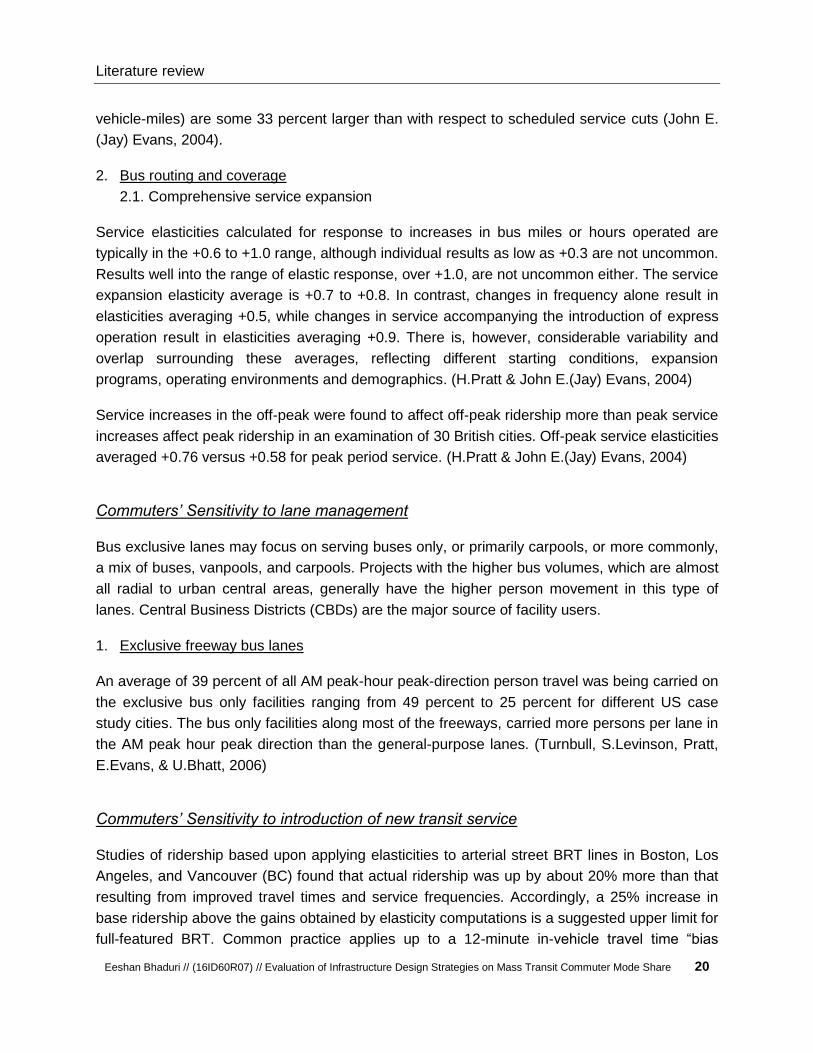
Figure 4-5 Distribution of income groups (a) 8 income bracket and (b) 4 income bracket vs modal shares
.................................................................................................................................................. 28
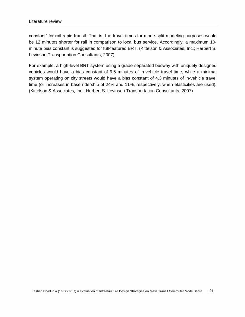
Figure 4-6 Distribution of education groups and modal shares .................................................................. 28
Figure 4-7 Distribution of household and modal shares ............................................................................ 29
Figure 4-8 Distribution of vehicle ownership and modal shares ................................................................. 30
Figure 4-9 Trip frequency for different trip purposes (both corridors combined) ....................................... 30
Figure 4-10 Trip frequency in peak and off-peak hour (both corridors combined) .................................... 31
Figure 4-11 Number of transfers vs. commuter percentage ...................................................................... 34
Figure 4-12 Mode type change vs commuter percentage ......................................................................... 34
Figure 4-13 Variable correlation square plot .............................................................................................. 35
Figure 4-14 kappa statistic for 10 model-validation run ............................................................................. 43
Figure 4-15 Observed vs. Predicted modal share for modes (a) Auto-Rickshaw, (b) Bus, (c) Subway and
(d) Train .................................................................................................................................... 44
Figure 4-16 Distribution of modal share by trip length (observed vs predicted) ........................................ 45
Figure 5-1 Study area (hatched) & network (existing & proposed) map of city of Kolkata Metropolitan
area ........................................................................................................................................... 46
Figure 5-2 Passenger demand vs. Stops (a) morning peak, (b) evening peak and (c) afternoon off-peak
.................................................................................................................................................. 49
Figure 5-3 Average speed (different modes) vs. Stops (a) morning peak, (b) evening peak and (c)
afternoon off-peak ..................................................................................................................... 50
Figure 5-4 Average total travel time vs. Time of day ................................................................................. 50
Figure 5-5 Average waiting time vs. Time of day ....................................................................................... 51

List of Figures
Eeshan Bhaduri // (16ID60R07) // Evaluation of Infrastructure Design Strategies on Mass Transit Commuter Mode Share IX
Figure 5-6 Average vehicle (comfortable) occupancy vs. Time of day ...................................................... 52
Figure 5-7 Passenger demand vs. Stops (a) morning peak, (b) evening peak and (c) afternoon off-peak
.................................................................................................................................................. 53
Figure 5-8 Average speed (different modes) vs. Stops (a) morning peak, (b) evening peak and (c)
afternoon off-peak ..................................................................................................................... 54
Figure 5-9 Average total travel time vs. Time of day ................................................................................. 55
Figure 5-10 Average waiting time vs. Time of day ..................................................................................... 56
Figure 5-11 Average vehicle (comfortable) occupancy vs. Time of day .................................................... 57
Figure 5-12 Change in commuter mode share in Corridors A and B predicted for scenarios ................... 67
Figure 5-13 Commuter mode share predicted for scenarios (a) auto-rickshaw available and (b) auto-
rickshaw not available............................................................................................................... 69
Figure 5-14 Change in commuter mode share predicted for scenario level 2.1 (a) above and (b) below 70
Figure 5-15 Change in commuter mode share predicted for scenario level 2.2 (a) above left, (b) above
right, (c) below left and (d) below right ..................................................................................... 72
Figure 5-16 Change in commuter mode share predicted for scenario level 2.3 (a) and (b) ...................... 73
Figure 5-17 Change in commuter mode share predicted for scenarios (a) auto-rickshaw available and (b)
auto-rickshaw not available ...................................................................................................... 74
Figure 5-18 Change in commuter mode share predicted for scenario level 2.1 (a) above and (b) below 76
Figure 5-19 Change in commuter mode share predicted for scenario level 2.2 (a) above left, (b) above
right, (c) below left and (d) below right ..................................................................................... 77
Figure 5-20 Change in commuter mode share predicted for scenario level 2.3 (a) and (b) ...................... 78

List of Tables
Eeshan Bhaduri // (16ID60R07) // Evaluation of Infrastructure Design Strategies on Mass Transit Commuter Mode Share X
List of Tables
Table 3-1 Summary of transit development policies (Jeffrey, 2018)........................................................... 16
Table 3-2 Factors contributing to satisfaction of transit trip ........................................................................ 18
Table 4-1 Average travel speed matrix for different modes & no. of records ............................................ 32
Table 4-2 Travel cost matrix for different modes ....................................................................................... 33
Table 4-3 Correlation between different variables ..................................................................................... 36
Table 4-4 MNL estimation results (R – ‘mlogit’ package) .......................................................................... 37
Table 4-5 Statistical summary of the MNL estimation (R – ‘mlogit’ package) ........................................... 38
Table 4-6 Re-estimation with first 10 attempts with random set comprising 80% of full dataset ............... 41
Table 4-7 Re-estimation results for all attempts (20 times) and statistical significance threshold ............ 41
Table 4-8 Full model comparison with model without constants and constants-only model ..................... 42
Table 4-9 Sample confusion matrix (validation run 4) ............................................................................... 43
Table 5-1 Cost and Time budget outline for different types of transit improvement strategies ................. 62
Table 5-2 Selected sub scenarios (capacity constraints) of scenario-1 (Improvement in network) ....... 63
Table 5-3 Selected sub scenarios (speed constraints) of scenario-1 (Improvement in network) ........... 64
Table 5-4 Selected sub scenarios of scenario-2 (Improvement in lane management) .......................... 65
Table 5-5 Selected sub scenarios of scenario-3 (Introduction of new transit service BRTS) .............. 66
Table 6-1 Summary of improvement strategies (in terms of modal shift) ................................................... 79

List of Abbreviations
Eeshan Bhaduri // (16ID60R07) // Evaluation of Infrastructure Design Strategies on Mass Transit Commuter Mode Share XI
List of Abbreviations
MT Mass transit
PT Public transit
PV Private Vehicle
IPT Intermediate public transport
RP Revealed preference
SP Stated preference
MNL Multinomial Logit
NL Nested Logit
ILM Incremental logit model
IIA Independence of irrelevant alternatives
BRTS Bus rapid transit system
LOS Level of service
Introduction
Eeshan Bhaduri // (16ID60R07) // Evaluation of Infrastructure Design Strategies on Mass Transit Commuter Mode Share 1
Chapter 1 - Introduction
This chapter lays the foundation for this thesis. The existing scenario has been briefly
described, which leads to the motivation for this research. It is followed by the problem
statement; and then research objective and scope have been quantized by the end of this
chapter. Expected deliverables and a basic outline of the project, are also a feature of this
chapter.
1.1 Motivation
1.1.1 Present scenario of transport sector in India
Indian cities have been traditionally dependent on buses as dominant mode of transport
because of its advantages to carry more people at a time and being economical as well. These
advantages had been facilitated by the mixed land use model that allows neighborhoods to
provide for all the facilities ranging from housing to educational institutions to retail and
healthcare. This in-turn has resulted in the minimizing of trip lengths as well as the decreased
dependence on personal motorized transport. The average trip length in medium and small size
cities is less than 5 km, as shown in below.
Figure 1-1 Travel mode share across population across different Indian cities (Ministry of Urban Development, Handbook of Urban Statistics, 2016)
Figure removed due to possible copyright infringements

Introduction
Eeshan Bhaduri // (16ID60R07) // Evaluation of Infrastructure Design Strategies on Mass Transit Commuter Mode Share 2
Such city/neighborhood design also encourages the use of non-motorized modes and public
transportation, which includes the para-transit modes (also referred to as intermediate public
transport modes) and consequently lowering the average trip lengths as is shown in below.
Figure 1-2 Percentage share of Trip lengths across different Indian cities (Ministry of Urban Development, Handbook of Urban Statistics, 2016)
Unfortunately though, the bus fleet size is degrading fast (20%-40% drop from 2000-2008) even
in big metros like Delhi, Mumbai, Kolkata (Ministry of Urban Development, Handbook of Urban
Statistics, 2016) as shown in whereas the private vehicle (PV) and intermediate public transport
(IPT) is increasing to fill the void.
Figure 1-3 Increase in vehicle population and Decline in STU fleet size (National Transport Development Policy Committee, 2014)
Figure removed due to possible copyright infringements
Figure removed due to possible copyright infringements
Introduction
Eeshan Bhaduri // (16ID60R07) // Evaluation of Infrastructure Design Strategies on Mass Transit Commuter Mode Share 3
Existing performance evaluation reports of traffic condition done by Indian Government itself
clearly shows a huge gap in ‘mass transport’ (MT) infrastructure, plagued by inadequate
capacity and financial reasons, specifically in Kolkata which includes (a) Depleting fleet size of
MT (b) Unreliable service of most MT services, and (c) Less or no coordination between
different MT modes (National Transport Development Policy Committee, 2014). The poor state
of MT modes in cities like Kolkata have been further magnified by IPT modes which act as a
competitor rather being an ideal feeder service which perhaps could be a solution to last mile
connectivity problem. In the absence of adequate provision of MT infrastructure especially in
cities like Kolkata, including public transport, congestion diseconomies outweigh the benefits of
agglomeration forcing people to switch to PV and IPT like auto-rickshaw.
1.1.2 Past work and research gap
Figure 1-4 Implication of BRTS across different continents (Ministry of Urban Development, Report of the High Powered Committee on Decongesting Traffic in Delhi, 2016)
For solution of the congestion problem different strategies are being taken up by Government of
India such as following:
I. Strategy I (Improving PT & Dis-Incentivizing use of PV)
Multi-modal integration & ITS
Bus service improvements
II. Strategy II (Road safety & Traffic improvement)
Road network optimization
III. Strategy III (Development of TOD)
It is agreed that BRTS is a proven solution across continents as we can find out from Figure 1-4
but at the same time it can be argued that where and when to implement BRTS can impact the
urban transport structure hugely as it is seen in the case of BRTS in Ahmedabad in India. In an
overall aspect Ahmedabad BRTS is an accepted success but it is not same for all the corridors.

Introduction
Eeshan Bhaduri // (16ID60R07) // Evaluation of Infrastructure Design Strategies on Mass Transit Commuter Mode Share 4
Figure 1-5 Implication of BRTS in Narol-Naroda corridor, Ahmedabad (KT & Munshi, 2015)
It can be found out from that after implication of BRTS corridor in Narol-Naroda stretch in
Ahmedabad, India, bicycle and walk modal share has dropped and motorbikes & Auto-
Rickshaw modal share has increased from the figure above, which is completely opposite to the
desired scenario. So now it is to be decided as a transportation planner what is the right way to
go for us - will we be taking bigger irrational goals or we should focus on small changes to make
a bigger impact.
Different literatures regarding the design of infrastructures as well as transport policies to attract
PV and IPT users back to public transit had been reviewed. Chakrabarti (2017) discusses
effective strategies for increasing transit's competitiveness relative to auto, and hence attracting
people from their own cars to public transits. It is being emphasized that parallel to the rail
network expansion and Transit oriented development across US cities investors need to put
much importance to key aspects of bus service quality like speed, frequency and reliability to
cause the more shift from private cars to transit. Although it just identifies the key aspects
through modeling not going in detail to the mode choice model and how will be the share of
modes in futuristic scenarios of implication of these parameters in case of nationwide mode
choice model.
Fatima & Kumar (2014) make point about the implication of public bus transit in Indian cities and
for the research purpose uses VISSIM for traffic simulation but the case study is majorly based
on the stated preference survey and no revealed preference survey is being taken to
understand the mode choice of existing scenario in detail. If we could have got a combined
stated and revealed preference survey the results could have been more reliable. Dissanayake
& Morikawa, (2010) and Anwar & Yang (2017) show with help of binary logistics model that a
direct bus service with hourly interval is more efficient strategy compared to Park & Ride service
causing approximately 4.7 times higher modal shift to MT.
Figure removed due to possible copyright infringements
Introduction
Eeshan Bhaduri // (16ID60R07) // Evaluation of Infrastructure Design Strategies on Mass Transit Commuter Mode Share 5
At the same time, it can be argued that there are very few studies which clearly deal with
multiple MT modes and multiple policies at same time which resembles better with our actual
mode choice behavior. That is why this thesis approaches to work on that focus area without
any pre-fixed bias about any transit policy.
1.2 Research aims and objectives
The broad aim of this research project is to facilitate the sustainable usage of bus transit in
Indian subcontinent condition. Hence the major objectives to realize this scenario are as
followed:
i. Measure current commuter behavior (mode choice model);
ii. Design future strategies (scenario development) and
iii. Predict the impact of strategies on user behavior (modal shift analysis)
The main tasks for achieving above mentioned objectives of the project are as followed:
i. To build a mode choice model for Public Transport users of 4 types of modes i.e. Train,
Subway, Bus (Public & Private) and Auto-Rickshaw (for both study corridors)
ii. To estimate the model with full dataset to encompass as much variation in mode choice
behavior as possible.
iii. To re-estimate the model with 80% of full dataset (random) and validate it with the rest
20% data for 10 times to remove the stochasticity.
iv. To Assess the shift in modal share to bus from other modes in 3 futuristic scenarios of
improved travel time & improved headway / frequency
v. To evaluate the transit improvement policies based on the predicted modal shift to bus
on the study corridor(s) as a representative of the city.
1.2.1 Scope
The research project starts with the aim of finding out impact of different service improvement
measures in shift of modal share to bus mode in two busy corridors in Kolkata, India to optimise
the strategic planning procedure. The scopes of the work are listed as below.
i. Majorly three types of dataset are collected in the case study survey –
a. Travel time survey
b. Public perception survey
c. Occupancy & Travel cost survey
ii. Travel time survey (total dataset size=45 for each corridor) had been done for 4 modes
(Train, Subway, Bus and Auto-Rickshaw). It’s worth mentioning that subway travel time

Introduction
Eeshan Bhaduri // (16ID60R07) // Evaluation of Infrastructure Design Strategies on Mass Transit Commuter Mode Share 6
data has been collected based on e-timetable and schedule variability for subway is
negligible. The survey comprises of the information regarding
a. Arrival time at each intermediate stop
b. Departure time at each intermediate stop
c. Waiting time in signal and,
d. Waiting time without signal
iii. Public perception survey (total dataset size=218) had been done for 4 modes (Train,
Subway, Bus and Auto-Rickshaw) which comprises of the information regarding
a. Personal Characteristics (Socio-economic character)
b. Household Characteristics
c. Trip Characteristics (including walking trip & Trip chaining details)
d. Satisfaction measures (point scale)
iv. Occupancy and Travel cost survey (total dataset size=60) had been done for 4 modes
(Train, Subway, Bus and Auto-Rickshaw) which comprises of the information regarding
a. Occupancy at peak and non-peak hour
b. Fare hierarchy
v. All the datasets were collected for 1-month period from 26th July, 2017 to 26th August,
2017 and in-spite of being it rainy season in Kolkata the survey was done mostly during
normal weather condition to minimize the effect of external factors in mode choice.
vi. The slot selection for the case-study hours were done based on literature reviews which
suggested to ignore weekends as well as Monday and Friday for having irregular travel
behaviour nature on those days. At the same time as many as 6 persons were chosen
for doing the public perception survey to remove the personal bias towards
documentation.
vii. The input would be used to setup a mode-choice model estimation framework, in which
various configurations of the variables are evaluated.
1.2.2 Limitation and Assumption
The limitations of the study can be summarised as below.
i. Absence of stated preference survey data for simulation of mode choice behavior of
public transport users in the improved scenarios.
ii. Absence of traffic volume survey so exact futuristic travel time cannot be obtained
through simulation in VISSIM though working with a certain range of (changed) travel
time in improved scenario will serve the purpose.
iii. Choice of corridor is not representative of whole Kolkata as the traffic as well as street
characters differ a lot across various corridors in Kolkata.
iv. Absence of dataset comprising Private Cars and Ola/Uber users in the survey as only
Public transport users’ datasets are captured in the Bus/Subway station surveys.

Introduction
Eeshan Bhaduri // (16ID60R07) // Evaluation of Infrastructure Design Strategies on Mass Transit Commuter Mode Share 7
v. Dataset size: Considering similar research works the dataset size was limited to
consider different mode choice variable at a requisite statistical significance level which
can cause the weak validation performance of the model.
1.3 Geographical scope: Case study corridors
Figure 1-6 Case Study Corridors (1. Tollygunje to Kalighat and 2. Garia to Gariahat)
Two (2) corridors/segments selected in Kolkata, West Bengal– one is from Tollygunje to
Rashbehari Crossing/ Kalighat Metro Station is approximately 3 Km and another is from Garia
to Gariahat market which is approximately 6.5 Km.
The area has highly mixed-use development with residential density high towards Tollygunje
and Garia and Recreation and Commercial activities are densified in the other end of the
segment. In between Garia and Gariahat market Jadavpur University is a major educational
institution whereas both the corridors are well connected with other parts of the city as well as
the proposed BRTS corridor.
Corridor A - Tollygunje to Rashbehari Crossing/ Kalighat Metro Station corridor (Deshapran
Sashmal Road) is 3 lane road for whole study length whereas Corridor B - Garia to Gariahat
market (Subodh Chandra Mallick Road) is a mix of 2 lanes and 3 lanes as Sukanto setu to
Garia stretch has width 2 lanes and sometimes less than that also. The schematic street
sections details are provided below for better understanding.

Introduction
Eeshan Bhaduri // (16ID60R07) // Evaluation of Infrastructure Design Strategies on Mass Transit Commuter Mode Share 8
Figure 1-7 Street section details of corridor A (3 lane wide)
Figure 1-8 Street section details of corridor B (2 lane wide stretch shown)
Introduction
Eeshan Bhaduri // (16ID60R07) // Evaluation of Infrastructure Design Strategies on Mass Transit Commuter Mode Share 9
1.4 Organisation of Report
As previously mentioned, this thesis aims to evaluate the transportation policies related to public
transit improvement for Kolkata district in West-Bengal state in India. This objective is achieved
in a structured manner. The report begins with,
Chapter 1 - by introducing the motivation behind the work and the present scenario. After which,
the objective, scopes and limitations have been outlined.
Chapter 2 - gives the outline of the approach which has been taken to achieve the final goal of
this thesis.
Chapter 3 - consists of literature review, in which all the basic concepts and necessary
terminologies in the context of this work is laid out. It ends with conclusions arrived upon after
vetting the existing literature.
Chapter 4 - steps for preparation of the database for building the logit model, which is the basic
input as it translates the case study area details into a format understood by the statistical
software, are laid out. This chapter also deals with model validation aspect.
Chapter 5 - features further application of the statistical software for futuristic scenario analysis,
and results and repercussions of those results are discussed in depth.
Chapter 6 - provides the concluding remarks along with the scope for further research on the
same topic.

Approach
Eeshan Bhaduri // (16ID60R07) // Evaluation of Infrastructure Design Strategies on Mass Transit Commuter Mode Share 10
Chapter 2 - Approach
This thesis is focused towards the mass transit that is being emphasized in urban planning for
the Indian cities especially the Million plus ones. The idea is to utilize a mode choice modeling
framework to estimate the impact of the service and infrastructure improvement measures in
terms of improved travel time and expanded peak hour on the segment’s commuter mode
share. This approach involves five major exercises:
1. Brainstorming research objectives and framing of the outline;
2. Designing survey instrument and conducting station-based survey over one-month period;
3. Formulation of a suitable mode choice model (considering small dataset size);
4. Prediction of choice probabilities in three futuristic scenarios with transit service
improvement measures using the mode choice mode and
5. Evaluation of different transit improvement strategies based on the modal shift inflicted by it.
The steps that have been adopted to execute this exercise are as following:
i. Review of the mode choice modeling framework;
ii. Review of studies on mass transit improvement strategies and travelers’ response to
different transportation system changes;
iii. Exploration of available data (survey records);
iv. Specification of model choice set, variables, and structure;
v. Estimation of model parameters and analysis of results;
vi. Development of prediction scenarios along with dataset preparation for prediction; and
vii. Scenario analysis for the prediction of impacts of service improvement measures.
An easier interpretable description of the thesis methodology is given in the following flowchart.
Figure 2-1 Flow chart of thesis methodology
Literature review
RP survey at transit
stops
Estimation & Validation of a MNL mode
choice model
Scenario development
(Bus LOS improvement)
Scenario analysis based on
modal shift to Bus
Policy recommen
dations

Literature review
Eeshan Bhaduri // (16ID60R07) // Evaluation of Infrastructure Design Strategies on Mass Transit Commuter Mode Share 11
Chapter 3 - Literature review
3.1 Discrete Choice Modeling Framework
The discrete choice framework instructs to model individual’s choice behaviour econometrically
with help of the principle of utility maximization (Ben-Akiva & Lerman, 1985). Alternatively
explained, individuals are modelled to choose the alternative with the highest utility compared to
other alternatives present. In the domain of transportation, utility represents the attractiveness of
an alternative which is expressed as a function of alternative’s attributes (Ortúzar & Willumsen,
2011). In this theory we assume that individuals (homogenous population) behave rationally, are
well informed about all alternatives and are provided with a mutually exclusive and collectively
exhaustive choice set (Ortúzar & Willumsen, 2011).
There are mainly two broad steps of discrete choice modeling. Firstly, each alternative is
assigned a utility in the form of a parameterized function expressed by its attributes and
unknown parameters (Ben-Akiva & Lerman, 1985). These unknown parameters are then
estimated from a sample of observed choices made by a set of individuals under similar choice
condition. These two steps – model specification and model estimation constitute the modeling
framework.
One of the important hurdle during model specification is to build the utility function where most
transport researchers assume an additive, linear-in-parameter function. The theory requires
researchers to assume a universal choice set and to assign each individual decision maker an
individual choice set based on his/ her travel time or cost budgets (Ben-Akiva & Lerman, 1985).
In general, these individual constraints are taken care by socio-economic characteristics into the
utility function.
Under this modeling framework, all individuals with the same attribute values and similar socio-
economic characteristics would choose same alternative, one with the highest utility. However,
in reality it’s not the same because individuals are not perfectly rational and models are not
perfect too. Therefore, to address this issue, a probabilistic choice approach based on random
utility theory is adopted where the utility function also has a stochastic nature (Oppenheim,
1995). Consequently, the utility function of an alternative i for an individual n, Uin, is expressed
as a combination of measurable, systematic component, Vin, and a random component, εin, as
shown in Equation 3.1.
Equation 3.1
Uin = Vin + εin (Ortúzar & Willumsen, 2011)

Literature review
Eeshan Bhaduri // (16ID60R07) // Evaluation of Infrastructure Design Strategies on Mass Transit Commuter Mode Share 12
In this equation, the systematic component, Vin, is the parameterized function of the observable
attributes of the alternative i which can be written as in Equation 3.2.
Equation 3.2
Vin = β1iX1in+ β2iX2in+ β3iX3in+………+ βkiXkin (Ortúzar & Willumsen, 2011)
Where, X1in, X2in, ……., Xkin are the k independent variables that include both attributes of the
alternative 𝑖 and socio-economic variables of the individual] n; and
β1i , β2i,…, βki are the unknown parameters which are assumed to be constant across
individuals, and may vary across alternatives.
In this utility form, the random component, εin, caters to all the unobserved variation among
individuals as well as other observational errors during survey. It is assumed as a random
variable which follows a certain probability distribution. This in turn makes the utility function
also random. Therefore the probability that an alternative is chosen is the alternative having
maximum utility amongst all (Ben-Akiva & Lerman, 1985). Considering a choice set containing
two alternatives I and j, the probability that the individual n chooses the alternative i, Pin, is the
probability that the utility of alternative i, Uin, is greater than or equal to the utility of alternative j,
Ujn.
Equation 3.3
Pin = Probability { Uin >= Ujn} (Ben-Akiva & Lerman, 1985)
When the utilities in Equation 3.3 are expressed in terms of their systematic and random
components, probability Pin, can be written as shown in Equation 3.4
Equation 3.4
Pin = Probability {(εin - εjn)>= (Vjn – Vin)} (Ben-Akiva & Lerman, 1985)
In order to calculate probabilities as described above, a certain probability distribution is
assumed for the random error components and then the β parameters are estimated using
maximum likelihood estimation (Ben-Akiva & Lerman, 1985) (Ortúzar & Willumsen, 2011).
There are different types of discrete choice models based on different assumptions made on the
distribution pattern of the random component. Out of those, the logit class of models are found
to be assuming a logistic distribution of the error components which makes it most widely used
type of model. Within the logit model class, multinomial logit (MNL) and nested logit (NL) are
most used discrete choice models employed in travel demand forecasting research work along
with specific use of incremental logit model in case of introduction of a new mode. That’s why
we briefly review those types in following sub chapters.

Literature review
Eeshan Bhaduri // (16ID60R07) // Evaluation of Infrastructure Design Strategies on Mass Transit Commuter Mode Share 13
3.1.1 Multinomial Logit
Multinomial logit model is the type of logit models which are applied to choice sets containing
more than two alternatives. Similar to other type of logit models, MNL also assumes logistic
distribution for error component. All individual error components are independent and Gumbel
distributed with a location parameter η and scale parameter µ > 0 (Ben-Akiva & Lerman, 1985).
When a constant term is added to the systematic utility component of the alternatives, η is set to
null. Now the probability that an individual n chooses an alternative I from a choice set Cn, Pin, is
expressed by MNL model as in Equation 3.5.
Equation 3.5
Pin = exp(µ Vin) /∑ exp(µ Vin)Cn𝑗 (Ben-Akiva & Lerman, 1985)
Here, the systematic utilities of alternatives, Vin and Vjn are linear-in-parameter as in Equation
3.5 with an additional constant term, and for convenience, the scale parameter 𝜇 is set to 1.
Another crucial aspect of the MNL model is the IIA property (Independence from Irrelevant
Alternatives) which states that when choice probabilities of two alternatives are non-zero, their
ratio is independent of any other alternative in the choice set (Ortúzar & Willumsen, 2011). This
property is evident from Equation 3.5. By virtue of this property, the addition or removal of an
alternative to or from the choice set has the same effect on every other alternative in the choice
set. But in reality, alternatives are not completely independent, for example, when new transit
operations are introduced in a city, current captive riders are more likely to switch to the new
service than current captive drivers are. This inability of MNL models to capture correlations
between alternatives is addressed in the nested logit modeling framework. Nevertheless, MNL
models are still applied in the majority of mode choice models owing to their simple
mathematical form, and ease of estimation and interpretation (Koppelman & Bhat, 2006).
3.1.2 Nested Logit
The nested logit model addresses the IIA problem by grouping together alternatives those are
similar and choice-making is a multi-step decision which is shown in Figure 3-1.
Figure 3-1 Sample nesting structure (Koppelman & Bhat, 2006)
Mode
Public transitBus
Rail
CarDrive alone
Shared ride

Literature review
Eeshan Bhaduri // (16ID60R07) // Evaluation of Infrastructure Design Strategies on Mass Transit Commuter Mode Share 14
The NL model assumes that the random error terms are shared between some alternatives
(Koppelman & Bhat, 2006). This makes the utility equation of a particular alternative bus (as an
example) as shown in below:
Equation 3.6
Ubus = Vpt + Vbus + εpt+ εbus (Koppelman & Bhat, 2006)
Where,
εpt = Common random component and, Vpt = Common observed component
Similar to MNL model here too the error components are assumed to follow a Gumbel
distribution but with a scale factor µpt, or more commonly θpt = 1 µpt⁄
The probability of choosing a nested alternative is based on the conditional probability of
choosing the nested alternative times the marginal probability of choosing the nest (Munizaga &
Ortuzar, 1999), as shown in the following equation:
Equation 3.7
Prbus = (Pr bus/pt) * Prpt
Where,
Equation 3.8
Pr bus/pt = 𝑒(𝑉𝑝𝑡+𝜃𝑝𝑡∗𝜏𝑝𝑡)/(𝑒𝑉𝑑𝑎+𝑒𝑉𝑠𝑟+𝑒(𝑉𝑝𝑡+𝜃𝑝𝑡∗𝜏𝑝𝑡)) and,
Equation 3.9
𝜏𝑝𝑡 = log[𝑒𝑉𝑏𝑢𝑠/𝜃𝑝𝑡 + 𝑒𝑉𝑟𝑎𝑖𝑙/𝜃𝑝𝑡]
The log sum parameter otherwise known as nesting coefficient, corresponds to how similar
alternatives are within a nest. It should vary between 0 and 1 (Koppelman & Bhat, 2006), where
0 represents perfect correlation making the model deterministic. The selection of an appropriate
nest structure for a model is done through reasonable judgement and statistical evidence. At the
same time proposed nests are tested against each other and the MNL model to find out better
representation of observed behavior.

Literature review
Eeshan Bhaduri // (16ID60R07) // Evaluation of Infrastructure Design Strategies on Mass Transit Commuter Mode Share 15
3.1.3 Incremental Logit
The development of incremental logit model can be mainly attributed to the fact that there is
scarcity of time and cost budget to build a new full-fledged model every time we analyses mode
choice of an area. Existing mode choice model remains essentially unchanged, only the
incremental adjustment (such as revised travel time or fare) is accounted for. Model was built to
test transit alternatives but could be used to test other modes as well. (Koppelman, Predicting
transit ridership in response to transit service changes, 1983). It’s also worth noting that IIA
problem also applies for ILM as it is not built as a nested mode choice model.
As we are more interested in introduction of BRTS as a part of scenario analysis while keeping
existing bus service same or improving, we will be focusing only on the ILM framework when
new transit service is introduced keeping existing one. The rideshare of new transit mode will be
as shown in following equation:
Equation 3.10
Pnew transit,t+1 =
{Pexist transit, t ∗ 𝑒(𝑆 𝑛𝑒𝑤 𝑡𝑟𝑎𝑛𝑠𝑖𝑡,𝑡+1−𝑆 𝑒𝑥𝑖𝑠𝑡 𝑡𝑟𝑎𝑛𝑠𝑖𝑡,𝑡)}
P exist transit, t ∗ [ 𝑒(𝑆 𝑛𝑒𝑤 𝑡𝑟𝑎𝑛𝑠𝑖𝑡,𝑡+1−𝑆 𝑒𝑥𝑖𝑠𝑡 𝑡𝑟𝑎𝑛𝑠𝑖𝑡,𝑡) + 𝑒(𝑆 𝑒𝑥𝑖𝑠𝑡 𝑡𝑟𝑎𝑛𝑠𝑖𝑡,𝑡+1−𝑆 𝑒𝑥𝑖𝑠𝑡 𝑡𝑟𝑎𝑛𝑠𝑖𝑡,𝑡)} + (1 − Pexist transit, t)
And the rideshare of the existing transit mode is shown in below:
Equation 3.11
Pnew transit,t+1 =
{Pexist transit, t ∗ 𝑒(𝑆 𝑒𝑥𝑖𝑠𝑡 𝑡𝑟𝑎𝑛𝑠𝑖𝑡,𝑡+1−𝑆 𝑒𝑥𝑖𝑠𝑡 𝑡𝑟𝑎𝑛𝑠𝑖𝑡,𝑡)}
P exist transit, t ∗ [ 𝑒(𝑆 𝑛𝑒𝑤 𝑡𝑟𝑎𝑛𝑠𝑖𝑡,𝑡+1−𝑆 𝑒𝑥𝑖𝑠𝑡 𝑡𝑟𝑎𝑛𝑠𝑖𝑡,𝑡) + 𝑒(𝑆 𝑒𝑥𝑖𝑠𝑡 𝑡𝑟𝑎𝑛𝑠𝑖𝑡,𝑡+1−𝑆 𝑒𝑥𝑖𝑠𝑡 𝑡𝑟𝑎𝑛𝑠𝑖𝑡,𝑡)} + (1 − Pexist transit, t)
Therefore, total share on transit can be calculated using Equation 3.12
Equation 3.12
Ptotal transit,t+1 = Pexist transit,t+1 + Pnew transit,t+1
Again, the new shares for other modes would be as following Equation 3.13 below.
Equation 3.13
P mode,t+1 = Pmode,t * 1−Ptotal transit,t+1
1−Ptotal transit,t

Literature review
Eeshan Bhaduri // (16ID60R07) // Evaluation of Infrastructure Design Strategies on Mass Transit Commuter Mode Share 16
3.2 Mass transit development strategies and ridership
3.2.1 Scenario worldwide – selected cities and transport policies overview
Urban transportation system is a vital cog in the wheel for its own economy as planned transport
connections have strong relationship with better infrastructure. It improves the planning
procedure of funding ensuring integration among mass transit, local economy and infrastructure
development. As different countries across the world have taken up different initiatives to
improve public transportation system, the Table 3-1 below provides the best ten initiatives.
Table 3-1 Summary of transit development policies (Jeffrey, 2018)
Id Case study Policy aim Location
1 Improving existing bus routes, time
tables and bus stops
Improve bus quality and service Nottingham,
UK
2 Integrating planning of bus service
with other mass transit modes
Improve bus quality and service Helsinki,
Finland
3 Authority reformation to directly
control bus service
Improve bus quality and service London, UK
4 Provision of long term funding
certainty for infrastructure
Encouraging investment in
transport sector
Paris, France
5 Funding transport projects through
local taxes, fees and charges
Cost-benefit alignment for
transport sector
UK (City
councils)
6 Utilisation of BIG data to improve Increase service efficiency London, UK
7 Sharing data to improve Increase service efficiency Dublin, Ireland
8 Creation of real time map of road
condition
Increase service efficiency Boston, USA
9 Increase in accessibility to commercial
hubs in the city centre
Provision of better links to city
centre from wider zones
Manchester,
UK
10 Introduction of bus system in a mid-
sized city
Provision of better links to city
centre from wider zones
Oregon, USA

Literature review
Eeshan Bhaduri // (16ID60R07) // Evaluation of Infrastructure Design Strategies on Mass Transit Commuter Mode Share 17
It can be observed that most of the planning policies are related with development as well as
improvement of service aspect of public transportation system rather than introducing altogether
a new transit. Another point to be noted is that most of the cities in the above mentioned list are
metropolitan with considerable population base which resembles better with Indian cities
compared to new cities around the world. Simultaneously, the implication of new transit service
also includes intensive designing of service infrastructure for sustainable level of service.
3.2.2 Mass transit improvement strategies
It is important to study different mass transit improvement strategies and their possible impact in
qualitative as well as quantitative manner in order to develop the scenarios at later stage of this
research study. Transit improvement strategies can be broadly divided into two groups – (1)
small/medium/large service improvement and (2) transit improvement along with support
strategies (e.g. ridership incentive, transit-oriented development etc.). Similarly, the impacts can
also be grouped into two types – (1) net impact and (2) marginal impact (considering impact
happening within excess capacity). Moreover, other type of grouping of impacts can also be –
(1) direct and (2) indirect/ leverage effect (e.g. accessible land use pattern, diverse transport
system etc.) (Kittelson & Associates, Inc.; Parsons Brinckerhoff; KFH Group, Inc; Texas A&M
Transportation Institute; ARUP, 2013).
To make transit better there can be four major approaches – (1) improves service quality, (2)
increases affordability, (3) provides basic mobility and (4) reduces auto travel. The types of
benefits associated with all these approaches can also be grouped into three categories – (1)
user benefits (e.g. convenience, speed, cost, financial saving), (2) mobility benefits (e.g.
Physically/socially/economically disadvantaged people) and (3) efficiency benefits (e.g.
Congestion cost reduction. road and parking facility, pollution emission). Therefore transit
availability based on quality of service concept can be subdivided into four types – (1) spatial
availability (e.g. pedestrian access, park and ride), (2) temporal availability (frequency,
passenger arrival pattern), (3) information availability and (4) capacity availability (Kittelson &
Associates, Inc.; Parsons Brinckerhoff; KFH Group, Inc; Texas A&M Transportation Institute;
ARUP, 2013). In a nutshell it can be inferred that most important factors in transit improvement
strategies for a corridor level transportation planning purpose, are as follows:
1) Mode and service concept
a) Type of transit (e.g. Carrying capacity, comfort etc.)
b) Type of service and operating hours (e.g. fare characteristics, special service etc.)
2) Operating environments
a) Service way (grade separated or not)
b) Service pattern (traffic characteristics and facility design)

Literature review
Eeshan Bhaduri // (16ID60R07) // Evaluation of Infrastructure Design Strategies on Mass Transit Commuter Mode Share 18
3) Operating pattern/ concept
a) Capacity
b) Speed
c) Reliability
3.2.3 Commuter response to transit trip satisfaction
The variables are identified to be significant factors for transit quality of service through different
on-board surveys, along bus routes with varying service characteristics (e.g., frequency,
loading, reliability, amenity provision) and customers were asked to rate their overall satisfaction
with their trip, along with their satisfaction about specific aspects of their trip (e.g., frequency,
reliability). The result (Kittelson & Associates, Inc.; Parsons Brinckerhoff; KFH Group, Inc; Texas
A&M Transportation Institute; ARUP, 2013) shows the factors contributing most to stated overall
satisfaction of the commuters with a transit trip as shown in Table 3-2 below.
Table 3-2 Factors contributing to satisfaction of transit trip
Rank A B C D E
1 Frequency Frequency Frequency Frequency Frequency
2 Waiting time Reliability Close to home Reliability Waiting time
3 Reliability Waiting time Reliability Close to home Close to
home
4 Close to home Close to home Waiting time Close to
destination Reliability
5 Service span Close to
destination
Close to
destination Waiting time Service span
6 Close to
destination Service span Service span
7 Friendly drivers
After extensive literature review on bus LOS improvement strategies as well as the factors those
play important role in increasing bus ridership, majorly three types could be identified – (1)
network improvement measures (transit scheduling, frequency, routing, signalling etc.), (2) lane
management (high occupancy, exclusive bus lane etc.) and (3) introduction of new transit
service (BRTS). The sensitivity of commuters to transit service are either expressed in terms of 1
1 Italics signifies replies given by more than 50% respondents and others by at least 33% respondents

Literature review
Eeshan Bhaduri // (16ID60R07) // Evaluation of Infrastructure Design Strategies on Mass Transit Commuter Mode Share 19
modal shift (increase in bus ridership) or elasticity (service elasticity of +0.8 indicates, for
example, a 0.8 percent increase and/or decrease in transit ridership in response to each 1
percent service increase and/ or decrease) (Kittelson & Associates, Inc.; Parsons Brinckerhoff;
KFH Group, Inc; Texas A&M Transportation Institute; ARUP, 2013).
Commuters’ Sensitivity to network improvement
Network improvement strategies can be broadly grouped as follows:
1. Transit scheduling and frequency
1.1. Bus frequency change
Both historical and more recent elasticities of bus service changes exhibit a service elasticity
average that is on the order of +0.5 (it can vary from +0.3 to 1.0). (John E. (Jay) Evans, 2004)
1.2. Service hour change
The one impact assessment conclusion that can be reasonably drawn is that both types of
service time change (weekday and weekend) contributes substantially to the outstanding
ridership response, reflected in a service elasticity of +1.14. (John E. (Jay) Evans, 2004)
1.3. Combined service frequencies
In situations where the provision of new or expanded express bus service has resulted in
increased overall frequency of service exhibiting service elasticities on the order of +0.9. A
combination of increased service and express runs may attract additional patronage — possibly
half again as much — as would a similar bus trip increase applied to local service alone. (John
E. (Jay) Evans, 2004)
1.4. Regularized schedule
The restructuring generally accomplished within the constraint that total bus service hours not
be increased by more than 4 percent increases ridership around 20%. (John E. (Jay) Evans,
2004)
1.5. Transit reliability change
In general, the effects on ridership of lack of reliability will be even more pronounced than the
increase in waiting time alone indicates. This effect is attributable to the uncertainty about if and
when the next vehicle will arrive and consequent anxiety and annoyance to passengers. London
Transport has estimated that elasticities with respect to “unplanned” service cuts (i.e., lost
Literature review
Eeshan Bhaduri // (16ID60R07) // Evaluation of Infrastructure Design Strategies on Mass Transit Commuter Mode Share 20
vehicle-miles) are some 33 percent larger than with respect to scheduled service cuts (John E.
(Jay) Evans, 2004).
2. Bus routing and coverage
2.1. Comprehensive service expansion
Service elasticities calculated for response to increases in bus miles or hours operated are
typically in the +0.6 to +1.0 range, although individual results as low as +0.3 are not uncommon.
Results well into the range of elastic response, over +1.0, are not uncommon either. The service
expansion elasticity average is +0.7 to +0.8. In contrast, changes in frequency alone result in
elasticities averaging +0.5, while changes in service accompanying the introduction of express
operation result in elasticities averaging +0.9. There is, however, considerable variability and
overlap surrounding these averages, reflecting different starting conditions, expansion
programs, operating environments and demographics. (H.Pratt & John E.(Jay) Evans, 2004)
Service increases in the off-peak were found to affect off-peak ridership more than peak service
increases affect peak ridership in an examination of 30 British cities. Off-peak service elasticities
averaged +0.76 versus +0.58 for peak period service. (H.Pratt & John E.(Jay) Evans, 2004)
Commuters’ Sensitivity to lane management
Bus exclusive lanes may focus on serving buses only, or primarily carpools, or more commonly,
a mix of buses, vanpools, and carpools. Projects with the higher bus volumes, which are almost
all radial to urban central areas, generally have the higher person movement in this type of
lanes. Central Business Districts (CBDs) are the major source of facility users.
1. Exclusive freeway bus lanes
An average of 39 percent of all AM peak-hour peak-direction person travel was being carried on
the exclusive bus only facilities ranging from 49 percent to 25 percent for different US case
study cities. The bus only facilities along most of the freeways, carried more persons per lane in
the AM peak hour peak direction than the general-purpose lanes. (Turnbull, S.Levinson, Pratt,
E.Evans, & U.Bhatt, 2006)
Commuters’ Sensitivity to introduction of new transit service
Studies of ridership based upon applying elasticities to arterial street BRT lines in Boston, Los
Angeles, and Vancouver (BC) found that actual ridership was up by about 20% more than that
resulting from improved travel times and service frequencies. Accordingly, a 25% increase in
base ridership above the gains obtained by elasticity computations is a suggested upper limit for
full-featured BRT. Common practice applies up to a 12-minute in-vehicle travel time “bias
Literature review
Eeshan Bhaduri // (16ID60R07) // Evaluation of Infrastructure Design Strategies on Mass Transit Commuter Mode Share 21
constant” for rail rapid transit. That is, the travel times for mode-split modeling purposes would
be 12 minutes shorter for rail in comparison to local bus service. Accordingly, a maximum 10-
minute bias constant is suggested for full-featured BRT. (Kittelson & Associates, Inc.; Herbert S.
Levinson Transportation Consultants, 2007)
For example, a high-level BRT system using a grade-separated busway with uniquely designed
vehicles would have a bias constant of 9.5 minutes of in-vehicle travel time, while a minimal
system operating on city streets would have a bias constant of 4.3 minutes of in-vehicle travel
time (or increases in base ridership of 24% and 11%, respectively, when elasticities are used).
(Kittelson & Associates, Inc.; Herbert S. Levinson Transportation Consultants, 2007)

Modeling Framework
Eeshan Bhaduri // (16ID60R07) // Evaluation of Infrastructure Design Strategies on Mass Transit Commuter Mode Share 22
Chapter 4 - Modeling Framework
The current model adopts a discrete choice modeling framework described in previous section
and is based on data from a Field Study done in Kolkata. The construction of the model and its
functioning is explained in this chapter. It gives an overview of the data used and demonstrate
the model specification and estimation respectively.
4.1 Design of survey
As different literature suggests, there are predominantly two approaches to analyze modal shift
– (1) revealed preference (RP) approach and (2) stated preference (SP) approach. Here RP
approach has been followed as it is based on actual mode choice behavior which suits better for
building a mode choice model. All those data were collected through bus station survey,
conducted along two busy arterial roads in Kolkata, India - one is three (3) lane wide while the
other one is a mix of two (2) and three (3) lanes. As found in different literatures on mode choice
model, there are typically three types of variables –
1) Alternative specific (e.g. travel time, waiting time, service headway etc.)
2) Individual specific (e.g. age, gender, income, car ownership etc.)
3) Trip specific (e.g. number of transfers, bus stop density, trip purpose etc.)
Accordingly, the questionnaire was prepared with two major sections – General data – (a) socio-
economic data and (b) household data and Travel data – (a) trip related information.
Simultaneously, there was another type of survey done on same corridors i.e. Corridor
characteristics survey which includes each of the following features for all four modes in peak
and off-peak hours -
1) Travel time between two nodes and in between consecutive stops in the study stretch
2) Number of stops served by any particular mode
3) Occupancy (number of people in any particular mode)
4) Boarding and alighting time of passengers on every stop
5) Boarding and alighting number of passengers on every stop
6) Waiting time in and without signal
Moreover, data of the existing signaling system (g/c ratio, curb volume, vehicle type share etc.)
of all major intersections in the study corridors was also collected from the research group
working in ‘Future of cities’ project in Civil Engineering department in IIT Kharagpur.

Modeling Framework
Eeshan Bhaduri // (16ID60R07) // Evaluation of Infrastructure Design Strategies on Mass Transit Commuter Mode Share 23
4.2 Execution of survey
The field survey was done over a period of one month from 26th July, 2017 to 26th August, 2017
in Kolkata. Each part of the survey work was evenly distributed amongst six interviewers
(Masters Students in IIT Kharagpur) to remove any kind of bias in the response. Whole of this
work had been done from Tuesday to Thursday of every week during the above-mentioned time
period as it was found in different literatures that the travel behaviour is different in weekends as
well as Monday and Friday from the general working weekdays. Although the survey period falls
within the monsoon period prevalent in this region, the survey days was more or less free of
environmental interference as selected intentionally.
4.3 Survey responses
4.3.1 Field Study
Available Dataset from the RP survey results -
Class I - General
• Persons (socio-economic)
1. Type of residence
2. Age
3. Gender
4. Occupation
5. Income
6. Driving license possession
• Household
1. Household size
2. No. Of working household members
3. Vehicle ownership

Modeling Framework
Eeshan Bhaduri // (16ID60R07) // Evaluation of Infrastructure Design Strategies on Mass Transit Commuter Mode Share 24
Class II – Travel (RP Data)
• Trips
1. Origin
2. Destination purpose
3. Travel cost
4. Travel time (in range)
5. Transport mode
6. Trip chains/legs
7. Use of household auto
8. Waiting time
9. Preference reason
4.3.2 Model Dataset
A total 211 trips with detailed information about trip legs were extracted from the available
survey dataset. 7 nos. of trip records were neglected for errors or insufficient data.
4.4 Model Specification
4.4.1 Choice Set
Categorization of modes: Mode Hierarchy
1. Train
2. Subway
3. Bus
4. Auto rickshaw
As one would expect, it can be observed in Figure 4-1 and Figure 4-2, “Auto-Rickshaws” are
dominant for short commutes, and longer commutes are predominantly made by “Train” and the
trips with intermediate trip lengths has a mixed share of all 4 modes. Interestingly, a significant
share of “Auto-Rickshaws” commuting already seems to prevail for trips up to 15 km.

Modeling Framework
Eeshan Bhaduri // (16ID60R07) // Evaluation of Infrastructure Design Strategies on Mass Transit Commuter Mode Share 25
At the same time, it should also be noticed that the number of trip records (frequency
distribution) are also decreasing with the trip length increasing which can cause the occasional
spikes in the modal share graph (data inflicted defects).
In the following Figure 4-3, the mode “Bus” is further classified into “Public” and “Private” and
“Public “Bus” is further classified into “AC” and “Non-AC” types.
Figure 4-1 Distribution of modal shares and total trips by trip length
Figure 4-2 Distribution of modal shares and total trips by trip length (Trip length bin size changed-2Km)

Modeling Framework
Eeshan Bhaduri // (16ID60R07) // Evaluation of Infrastructure Design Strategies on Mass Transit Commuter Mode Share 26
Figure 4-3 Distribution of modal shares and total trips by trip length (Bus is further classified)
The present aim is to model the individual choice preferences leading to the above mode share
patterns. The explanatory variables used to achieve this are discussed in the next section.
4.4.2 Explanatory variables
1. Individual characteristics
2. Journey characteristics
3. Transport facility characteristics
Individual
Type of residence
Age
Gender
Occupation
Income
Vehicle ownership
Journey
Origin
Destination
Purpose
Trip chains/legs
Waiting time in stop
Time of day(peak/off)
Transport facility
Travel time(in range)
Travel cost
Preference reason

Modeling Framework
Eeshan Bhaduri // (16ID60R07) // Evaluation of Infrastructure Design Strategies on Mass Transit Commuter Mode Share 27
Age and Gender
Age and gender are the two most common individual-specific variables considered in mode
choice models (Fatima & Kumar, 2014). Among the respondents 68.3% are males and 31.7%
are females. In this model dataset, we find most male as well female population to be in 20-55
years categories which is expected as this age-group bracket is most active road users. The
frequency distribution of male and female commutes in the dataset by their ages is depicted.
(a) (b)
Figure 4-4 Distribution of (a) age groups and (b) gender
Income
Individuals’ choice preferences are greatly influenced by their income budgets (Fatima & Kumar,
2014) (Chakrabarti, 2017). Income Groups are clubbed in the following way. In Figure 4-2 (b),
each of the consecutive groups are clubbed together to find a smoother pattern.
Monthly Income 1 None 2 < 5000 INR 3 >5000 - 10000 INR 4 >10000 - 20000 INR 5 >20000 - 30000 INR 6 >30000 - 40000 INR 7 >40000 - 50000 INR 8 >50000 INR
It should also be considered that here only individual income is considered not household
therefore it does not give a clear picture of those who can afford high travel cost despite earning
less e.g. Students from high income households.
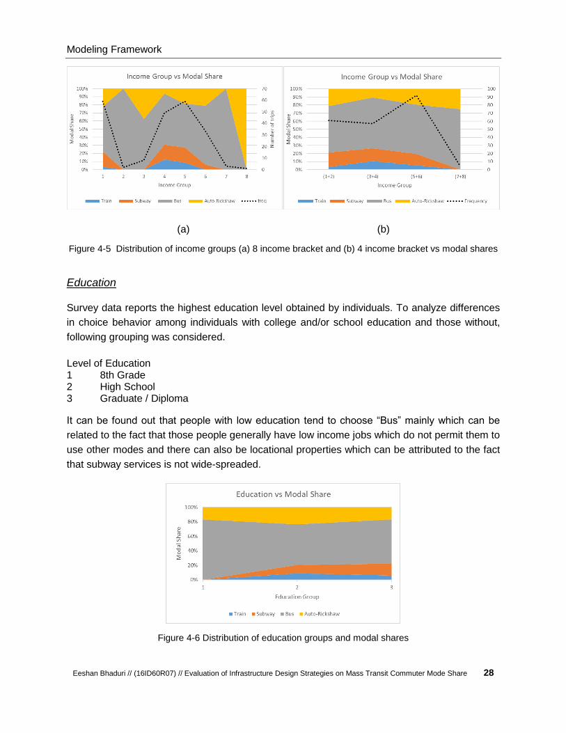
Modeling Framework
Eeshan Bhaduri // (16ID60R07) // Evaluation of Infrastructure Design Strategies on Mass Transit Commuter Mode Share 28
(a) (b)
Figure 4-5 Distribution of income groups (a) 8 income bracket and (b) 4 income bracket vs modal shares
Education
Survey data reports the highest education level obtained by individuals. To analyze differences
in choice behavior among individuals with college and/or school education and those without,
following grouping was considered.
Level of Education 1 8th Grade 2 High School 3 Graduate / Diploma
It can be found out that people with low education tend to choose “Bus” mainly which can be
related to the fact that those people generally have low income jobs which do not permit them to
use other modes and there can also be locational properties which can be attributed to the fact
that subway services is not wide-spreaded.
Figure 4-6 Distribution of education groups and modal shares

Modeling Framework
Eeshan Bhaduri // (16ID60R07) // Evaluation of Infrastructure Design Strategies on Mass Transit Commuter Mode Share 29
Household size and number of working household members
Household attributes like household size, number of children and number of employed people
have an influence on individuals’ choice of mode. For instance, household members may
combine or chain individual trips, making auto travel convenient. To capture this effect, these
variables were proposed for consideration in the model. In this model dataset, there is a
tendency of using auto-rickshaw for people with lower household size and more people using
subway with household size 3. The sudden fall in the train share in group of household size 5
can be data induced defect also.
Figure 4-7 Distribution of household and modal shares
Vehicle ownership
Having access to an auto significantly increases one’s propensity to drive to work. To capture
this, auto availability for individuals’ in the dataset was proposed to be evaluated as the number
of autos available to the individual calculated as given following equation
Vehicle ownership = Number of household vehicles (2 wheelers + 4 wheelers) / Number of
household members possessing driver’s license.
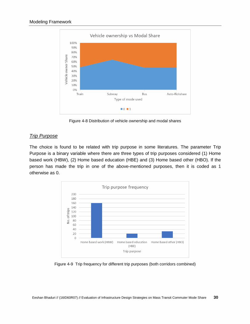
Modeling Framework
Eeshan Bhaduri // (16ID60R07) // Evaluation of Infrastructure Design Strategies on Mass Transit Commuter Mode Share 30
Figure 4-8 Distribution of vehicle ownership and modal shares
Trip Purpose
The choice is found to be related with trip purpose in some literatures. The parameter Trip
Purpose is a binary variable where there are three types of trip purposes considered (1) Home
based work (HBW), (2) Home based education (HBE) and (3) Home based other (HBO). If the
person has made the trip in one of the above-mentioned purposes, then it is coded as 1
otherwise as 0.
Figure 4-9 Trip frequency for different trip purposes (both corridors combined)

Modeling Framework
Eeshan Bhaduri // (16ID60R07) // Evaluation of Infrastructure Design Strategies on Mass Transit Commuter Mode Share 31
Time of day (peak / off-peak)
The choice of mode is expected to be affected by the time of day, especially by traffic peak
hours. Given an opportunity, travelers would try to avoid trips during peak hours to escape
congestion on roads and crowds in transit. Their effect could be observed in the proposed
model application with the help of a dummy variable differentiating peak-hour trips from off-peak
hour trips. Although the following Figure 4-10 shows the number of survey records collected in
each of the three phases of a day. Hence, its essentially a property of survey rather than the
commuters in that context.
For this, trip start times given in the survey data grouped as follows were used -
Trips made in time groups 08:00 to 11:00 and 17:00 to 20:00 were considered as peak-hour
trips, represented by 1, and trips starting during 14:00 to 17:00 time group was marked 0.
Figure 4-10 Trip frequency in peak and off-peak hour (both corridors combined)
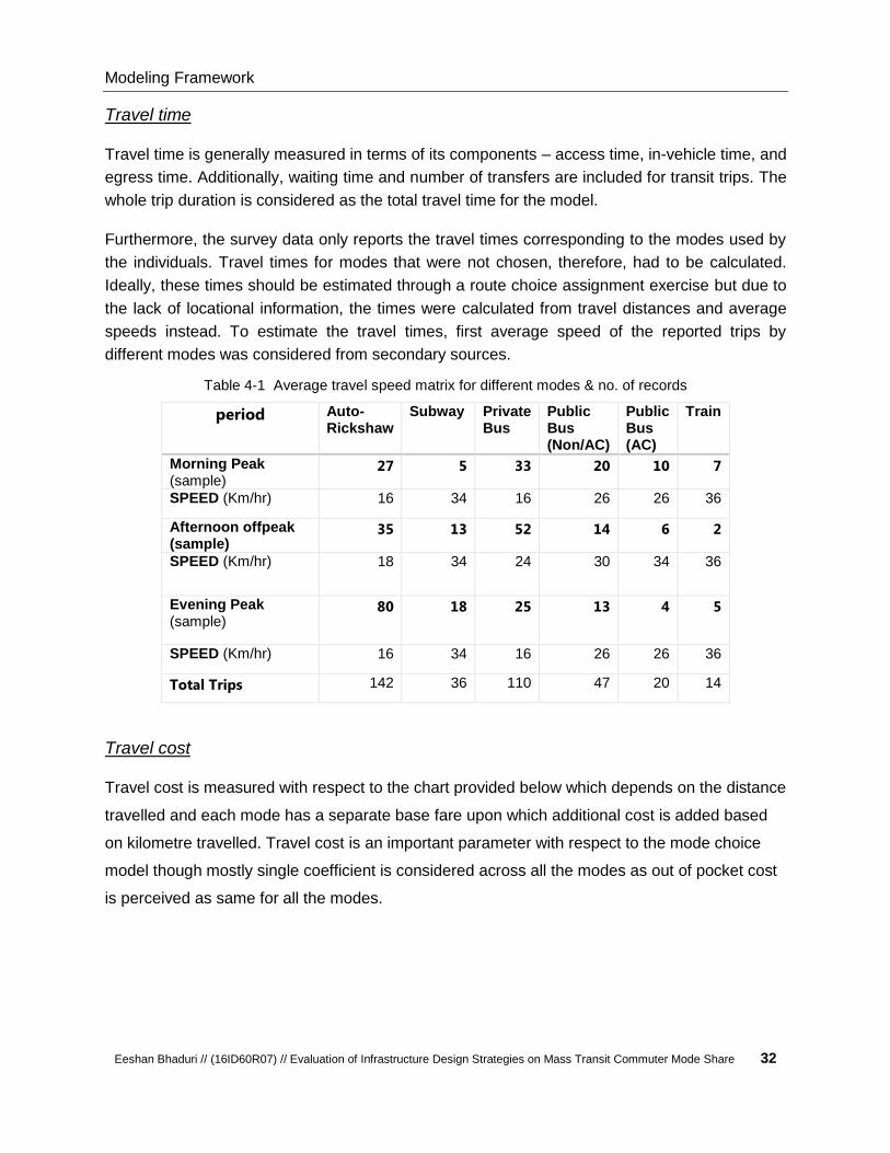
Modeling Framework
Eeshan Bhaduri // (16ID60R07) // Evaluation of Infrastructure Design Strategies on Mass Transit Commuter Mode Share 32
Travel time
Travel time is generally measured in terms of its components – access time, in-vehicle time, and
egress time. Additionally, waiting time and number of transfers are included for transit trips. The
whole trip duration is considered as the total travel time for the model.
Furthermore, the survey data only reports the travel times corresponding to the modes used by
the individuals. Travel times for modes that were not chosen, therefore, had to be calculated.
Ideally, these times should be estimated through a route choice assignment exercise but due to
the lack of locational information, the times were calculated from travel distances and average
speeds instead. To estimate the travel times, first average speed of the reported trips by
different modes was considered from secondary sources.
Table 4-1 Average travel speed matrix for different modes & no. of records
period Auto-Rickshaw
Subway Private Bus
Public Bus (Non/AC)
Public Bus (AC)
Train
Morning Peak (sample)
27 5 33 20 10 7
SPEED (Km/hr) 16 34 16 26 26 36
Afternoon offpeak (sample)
35 13 52 14 6 2
SPEED (Km/hr) 18 34 24 30 34 36
Evening Peak (sample)
80 18 25 13 4 5
SPEED (Km/hr) 16 34 16 26 26 36
Total Trips 142 36 110 47 20 14
Travel cost
Travel cost is measured with respect to the chart provided below which depends on the distance
travelled and each mode has a separate base fare upon which additional cost is added based
on kilometre travelled. Travel cost is an important parameter with respect to the mode choice
model though mostly single coefficient is considered across all the modes as out of pocket cost
is perceived as same for all the modes.

Modeling Framework
Eeshan Bhaduri // (16ID60R07) // Evaluation of Infrastructure Design Strategies on Mass Transit Commuter Mode Share 33
Table 4-2 Travel cost matrix for different modes
Auto-Rickshaw Subway Bus Train
Dist_slab
(Km)
Fare
(INR)
Dist_slab
(Km)
Fare
(INR)
Dist_slab
(Km)
Fare
(INR)
Dist_slab
(Km)
Fare
(INR)
0 6 0 5 0 7 0 5
1 7 5 10 3 8 5 5
2 8 10 15 6 10 10 5
3 9 15 20 10 12 15 5
4 10 20 25 14 14 20 5
5 11 25 30 18 16 25 10
6 12 30 35 22 18 30 10
7 13 35 40 26 20 35 10
8 14 40 45 30 22 40 10
9 15 34 24 45 15
10 16 38 26 50 15
11 17 42 28 55 15
12 18 60 15
13 19 65 20
14 20 70 20
15 21 75 20
16 22 80 20
17 23
18 24
19 25
20 26

Modeling Framework
Eeshan Bhaduri // (16ID60R07) // Evaluation of Infrastructure Design Strategies on Mass Transit Commuter Mode Share 34
Number of transfers
Figure 4-11 Number of transfers vs. commuter percentage
Number of transfers is another important trip specific variable which has a negative impact on
choosing a mode if one needs to break his/her trip more. It can be observed from Figure 4-11
that most people have 3 transfers (2 transfers are minimum as access & egress modes are
different from main trip mode for every record). It is worth noting as trip chaining happens
despite several overlapping bus routes running on both the corridors.
Mode type change (during a single trip)
Figure 4-12 Mode type change vs commuter percentage
The Figure 4-12 above can be studied in conjunction with Figure 4-11 as both of them indicate
to the fact that majority of the commuters need to break their trip at least once which in turn
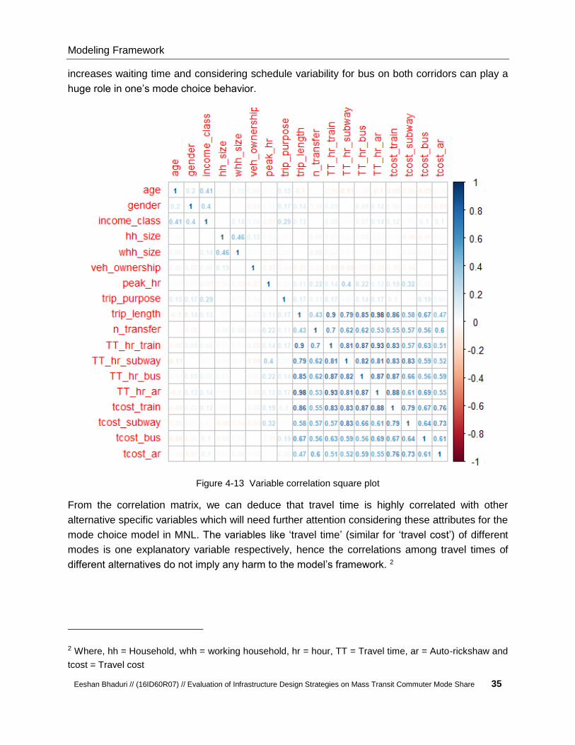
Modeling Framework
Eeshan Bhaduri // (16ID60R07) // Evaluation of Infrastructure Design Strategies on Mass Transit Commuter Mode Share 35
increases waiting time and considering schedule variability for bus on both corridors can play a
huge role in one’s mode choice behavior.
Figure 4-13 Variable correlation square plot
From the correlation matrix, we can deduce that travel time is highly correlated with other
alternative specific variables which will need further attention considering these attributes for the
mode choice model in MNL. The variables like ‘travel time’ (similar for ‘travel cost’) of different
modes is one explanatory variable respectively, hence the correlations among travel times of
different alternatives do not imply any harm to the model’s framework. 2
2 Where, hh = Household, whh = working household, hr = hour, TT = Travel time, ar = Auto-rickshaw and
tcost = Travel cost

Modeling Framework
Eeshan Bhaduri // (16ID60R07) // Evaluation of Infrastructure Design Strategies on Mass Transit Commuter Mode Share 36
Table 4-3 Correlation between different variables
Id Variables Variables with
correlation (>0.50)
Variables with correlation (0.25 -
0.50) Remarks
1 age
income_class
2 gender
income_class
3 income_class age
gender
4 hh_size
whh_size
5 whh_size
hh_size
6 veh_ownership
7 peak_hr tcost_subway
TT_hr.subway
8 trip_purpose
income_class
9 trip_length
tcost
high to low from train to ar
TT_hr
Very high for all 4 modes
n_transfer
10 n_transfer
tcost
approx. same for all 4 modes
TT_hr
approx. same for all 4 modes
trip_length
11 TT_time_hr
tcost
high to low from train to ar
n_transfer
trip_length
12 tcost
TT_hr
n_transfer
trip_length
It’s worth noting that the variables considered in the final mode choice equation are not even
having medium correlation amongst themselves. The variables inside the coloured boxes are
the ones considered for the final model. The variables are as following:
I. age,
II. travel time in hours,
III. peak hour,
IV. vehicle ownership and
V. trip purpose.

Modeling Framework
Eeshan Bhaduri // (16ID60R07) // Evaluation of Infrastructure Design Strategies on Mass Transit Commuter Mode Share 37
4.4.3 Results and Discussion
An MNL estimation using mlogit package with variables is called in R-Studio, the calling
expression is as follows:
Equation 4.1
mlogit (choice alternative specific variable | individual specific variable | alternative specific
variables with coeffcients differing across alternatives, data = dataset)
Table 4-4 MNL estimation results (R – ‘mlogit’ package)
Variable(s) Estimate Pr(>|t|) Significance
bus:(intercept) 2.61449 5.87e-07 ***
subway:(intercept) -1.01066 0.13611
train:(intercept) -2.24903 2.70e-09 ***
TT_hr -6.93211 < 2.2e-16 ***
bus * peak_hr -0.95616 0.08372 .
subway * peak_hr -1.04916 0.0667 .
subway * (veh_ownership)^2 -1.06393 0.20352
bus * age_2 0.9606 0.06526
.
subway * age_2 1.17498 0.04921 *
subway * trip_HBW -1.14735 0.03807 *
As already explained in sub-chapter 3.1.1 utilities are comprised of a measurable systematic
component and a random error component. Systematic components are expressed as additive
linear-in-parameter functions of known explanatory variables and unknown parameters, and
random components are assumed to follow a certain probability distribution. Under this
framework, the utilities of the four alternatives of the model’s choice set are written as follows –3
3 *** 99.9% significance level, ** 99% significance level, * 95% significance level, . 90% significance level

Modeling Framework
Eeshan Bhaduri // (16ID60R07) // Evaluation of Infrastructure Design Strategies on Mass Transit Commuter Mode Share 38
Equation 4.2
Umode = Vmode + εtmode
The expressions for final mode choice equations for all four modes becomes,
Equation 4.3
Ubus = 2.61449 – 6.93 * TT_hrbus – 0.95616 * peak_hr + 0.9606 * age_2
Usubway = -1.01066 – 6.93 * TT_hrsubway – 1.04916 * peak_hr - 1.06393 * veh_ownership
+ 1.17498* age_2 – 1.14735 * trip_HBW
Utrain = -2.24903 – 6.93 * TT_hrtrain
Uauto-rickshaw = 0– 6.93 * TT_hrauto-rickshaw
Table 4-5 Statistical summary of the MNL estimation (R – ‘mlogit’ package)
No. of Observations 211
No. of iterations 6
Log-Likelihood: -134.19
McFadden R2: 0.39928
Likelihood ratio test:
chisq
-178.38(p.value = < 2.22e-16)
The complete result output of the estimation from R is shown in Appendix B for further
reference. The estimation was performed with the mode auto as the reference as it is the most
represented. The estimates are hence to be understood with respect to Auto-Rickshaw
considered as the base mode. A discussion of the results is as follows:
Total Travel Time (variable id: TT_hr)
The total travel time for 3 modes (Subway, Bus & Auto-rickshaw) is constantly negative when
different coefficients for each mode is taken in the estimation of the mode choice model but it
comes positive for the mode train which is counter-intuitive that is why a single coefficient
across all the modes is taken for the parameter/ variable of total travel time.

Modeling Framework
Eeshan Bhaduri // (16ID60R07) // Evaluation of Infrastructure Design Strategies on Mass Transit Commuter Mode Share 39
In the beginning of estimation process when In-vehicle travel time and waiting time were taken
separately then in vehicle travel time coefficient in estimation was turning out to be positive
which is counter intuitive and cannot be explained from any secondary resource also so the new
variable total travel time is taken which is sum of those two alternative specific variables.
Age (variable id: age_2)
Age is an individual specific variable which is found to be statistically significant (relative) in
case of 2 modes – Bus and Subway but not for the mode Train. The variable ‘age’ has been
grouped into 4 categories – (1) 0 - <20 years, (2) 20 – 35 years, (3) 35 – 60 years and (4) >60
years based on in general education and retirement age prevailing in the region. As expected
according to different literature review and by intuition, the sign of the variable is positive which
suggests that as individuals are young, they prefer to use transit and subway as those options
are more cost-saving (more fitting to their income strata) and they are physically better capable
to use underground subway stations as most of it lack escalators/elevators, a problem for aged
persons.
Peak Hour (variable id: peak_hr)
Peak hour is another in trip specific variable which is also found to be statistically significant
(relative) in case of 2 modes – Bus and Subway but not for the mode Train. Similar to gender
parameter the variable Peak hour is taken to be as a Binary/dummy variable (for peak hour
value =1 or for non-peak hour value=0).
Expectedly the sign is negative for the parameter in case of both the alternatives – bus and
subway and it can also be supported from different literature (Appendix A). At the same time for
the mode subway the value is more negative which can also be supported with the analogy that
the overcrowding aspect during peak hour is huge in case of subway compared to bus which is
proven through the peak hour occupancy study during case study analysis.
Trip Purpose (variable id: trip_HBW)
Trip purpose is another individual specific variable which is found to be statistically significant
only for 1 mode - Subway but not for the mode Bus as well as Train. The variable Trip Purpose
is a binary variable as it has been coded for three major trip purposes – home based work,
home based education and home based other trips.
Modeling Framework
Eeshan Bhaduri // (16ID60R07) // Evaluation of Infrastructure Design Strategies on Mass Transit Commuter Mode Share 40
Though the sign of the coefficient is being intuitive as it’s showing a negative sign which can be
explained by the real-life situations like overcrowding as well as long queue for subways during
office hours.
Vehicle Ownership (variable id: veh_ownership)
Vehicle ownership is another individual specific variable which is found to be statistically
significant only for 1 mode - Subway but not for the mode Bus as well as Train. In fact, we also
use square function of the parameter which makes the overall statistical significance of the
model better.
Logically, the availability of an auto and/or motorbike reduces one’s tendency to use the other
modes. That is why the negative sign in the coefficient is very much intuitive.
Mode specific constants
The mode-specific constants shown in the results capture the effects of the unobserved
variables and measurement errors. auto-rickshaw has a constant value of 0 because it is the
base mode. Only one of the other three modes have positive constant- Bus and two have
negative constants - subway and train relative to auto, indicating that all else being equal, Train
is the least likely to be chosen, followed by subway and auto-rickshaw.
The mode train takes the highest constant as it is the least represented in the dataset, and its
attributes were perhaps not well captured by the model. At the same time the negative constant
for subway can be attributed to the fact that the city currently has only one corridor and
significant part of the city has poor/weak accessibility to it which is a major influential factor in
mode choice. To estimate the accuracy of the model fit, choice probabilities will be predicted for
the same model dataset using the estimated parameters at a later stage of estimation process.
However, one should be careful about the fact that the model does not consider ‘car’ mode
although one’s general intuition indicates that bus mode will only attract more ridership from
‘car’ mode as only improvement in service quality has been planned for bus. It should also be
kept in mind that the model could not perform equally well for all the modes in validation tests
and if there was a large dataset, the model probably could have considered more explanatory
variables with requisite statistical significance.

Modeling Framework
Eeshan Bhaduri // (16ID60R07) // Evaluation of Infrastructure Design Strategies on Mass Transit Commuter Mode Share 41
4.4.4 Re-estimation of Logit model
The dataset size for the estimation process was not large as compared to other models
prepared in similar kind of research therefore to build confidence in the signs and magnitudes of
constant as well as variables those were selected in the mode choice model, built based on the
full dataset (211 nos. data), an attempt was taken to re-estimate 10 times with same variables
for 80% of full dataset size (169 nos. data). In each of the attempts the survey records were
selected randomly with help of excel random number generation.
As an aggregated result of all those 10 attempts it can be found that R2 and Log-likelihood value
has (+/-) 4.26% and (+/-) 5.81% percentage standard deviation respectively which indicates that
there is not any significant departure from mean value. In the same line when percentage
standard deviation for the magnitude of mode specific constants are calculated, those were
observed to be (+/-) 6.19%, (+/-) 37.64% and (+/-) 10.78% respectively for bus, subway and
train. The deviation for subway mode is high probably because one corridor has significantly
better accessibility to subway and it may occur due to random selection that re-estimation
dataset consists of significant higher share of any particular corridor dataset. Although in every
case the signs and the mean value is consistent with the full dataset model.
Table 4-6 Re-estimation with first 10 attempts with random set comprising 80% of full dataset
Table 4-7 Re-estimation results for all attempts (20 times) and statistical significance threshold
Model
run id R^2
Log-
Likelihood bus subway train
bus subway bus subway
1 0.384 -107.95 2.89 -1.7 -2.34
2 0.388 -105.65 2.38 -1.52 -2.75
3 0.390 -113.51 2.51 -0.91 -2.26
4 0.383 -113.06 2.53 -0.6 -2.07
5 0.397 -106.12 2.71 -0.94 -2.21
6 0.393 -106.01 2.51 -1.14 -2.22
7 0.411 -105.03 2.54 -1.21 -2.48
8 0.391 -110.8 2.83 -0.32 -1.97
9 0.361 -116.82 2.41 -0.85 -2.1
10 0.428 -92.838 2.59 -1.35 -2.71
Intercept/Constant
all modes subway subway
Trip purpose
(trip_HBW)
Coeff. = Negative
Trip specific coefficientAlt. specific coeff.
Total Travel time
(TT_hr)
Coeff. = Negative
Age
(age_2)
Coeff. = Positive
Vehicle Occupancy
(veh_occupancy^2)
Individual specific coefficient
Coeff. = Negative
Peak Hour
(peak_hr)
Coeff. = Negative
Pr(>|t|) < 0.1017 15 14 11
Pr(>|t|) < 0.252 3 6 7
Pr(>|t|) > 0.251 2 0 2
0 10
Frequency for high
significance
Frequency for medium
significance
20 6 15
Frequency for
insignificance0 4 2
3
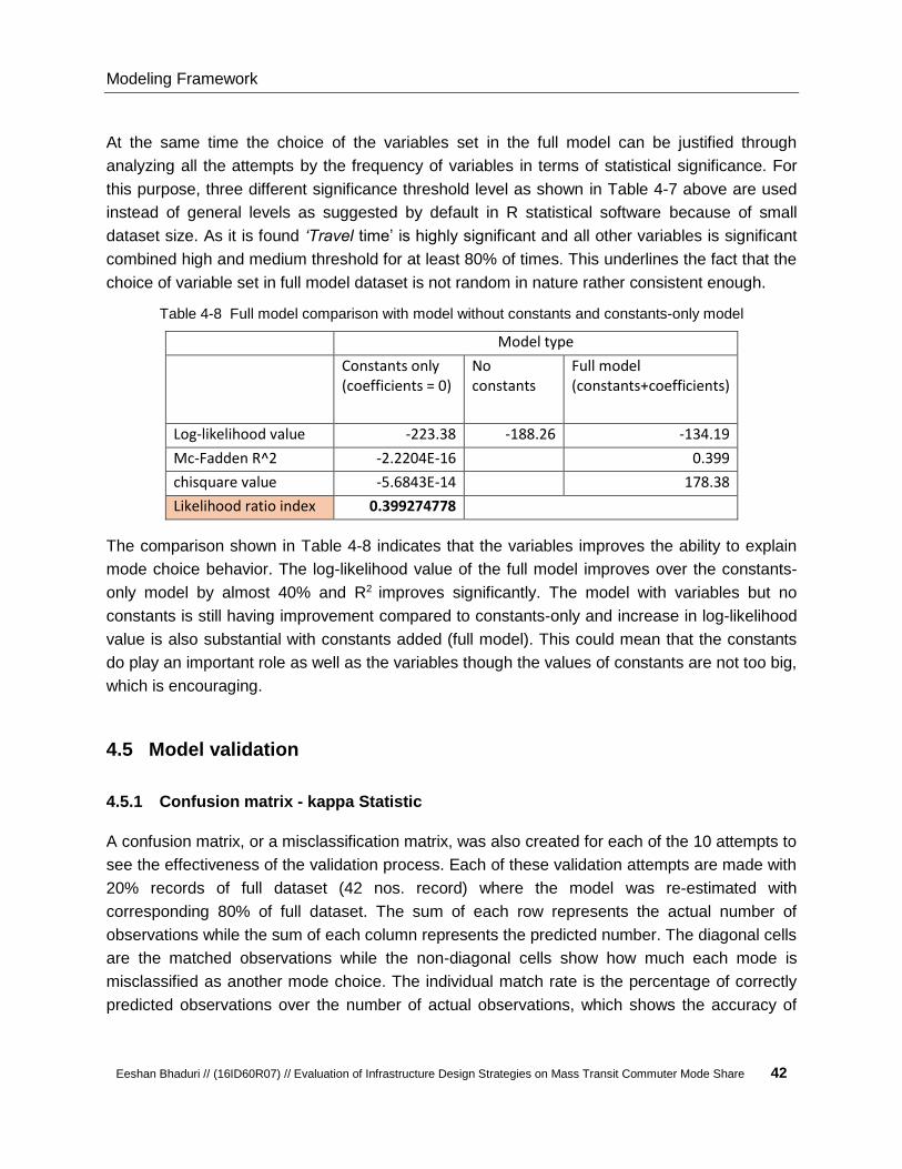
Modeling Framework
Eeshan Bhaduri // (16ID60R07) // Evaluation of Infrastructure Design Strategies on Mass Transit Commuter Mode Share 42
At the same time the choice of the variables set in the full model can be justified through
analyzing all the attempts by the frequency of variables in terms of statistical significance. For
this purpose, three different significance threshold level as shown in Table 4-7 above are used
instead of general levels as suggested by default in R statistical software because of small
dataset size. As it is found ‘Travel time’ is highly significant and all other variables is significant
combined high and medium threshold for at least 80% of times. This underlines the fact that the
choice of variable set in full model dataset is not random in nature rather consistent enough.
Table 4-8 Full model comparison with model without constants and constants-only model
Model type
Constants only (coefficients = 0)
No constants
Full model (constants+coefficients)
Log-likelihood value -223.38 -188.26 -134.19
Mc-Fadden R^2 -2.2204E-16 0.399
chisquare value -5.6843E-14 178.38
Likelihood ratio index 0.399274778
The comparison shown in Table 4-8 indicates that the variables improves the ability to explain
mode choice behavior. The log-likelihood value of the full model improves over the constants-
only model by almost 40% and R2 improves significantly. The model with variables but no
constants is still having improvement compared to constants-only and increase in log-likelihood
value is also substantial with constants added (full model). This could mean that the constants
do play an important role as well as the variables though the values of constants are not too big,
which is encouraging.
4.5 Model validation
4.5.1 Confusion matrix - kappa Statistic
A confusion matrix, or a misclassification matrix, was also created for each of the 10 attempts to
see the effectiveness of the validation process. Each of these validation attempts are made with
20% records of full dataset (42 nos. record) where the model was re-estimated with
corresponding 80% of full dataset. The sum of each row represents the actual number of
observations while the sum of each column represents the predicted number. The diagonal cells
are the matched observations while the non-diagonal cells show how much each mode is
misclassified as another mode choice. The individual match rate is the percentage of correctly
predicted observations over the number of actual observations, which shows the accuracy of

Modeling Framework
Eeshan Bhaduri // (16ID60R07) // Evaluation of Infrastructure Design Strategies on Mass Transit Commuter Mode Share 43
predictions. The aggregate match rate is the total number of predicted observations, correctly
and incorrectly predicted, over the actual number of observations per mode.
Table 4-9 Sample confusion matrix (validation run 4)
It can be observed from Table 4-9 that the model has quite good aggregate match rate and
moderately good individual match rate too. If all the validation attempts are considered, then a
high misclassification individual rate can be found for the mode train in almost all the cases and
in some attempts for other modes subway and auto-rickshaw. It seems most train trips are
misclassified as subway trips, which may indicate these modes share many similar
characteristics. This could also be due to heavy dominance of the bus mode and very low
number of observations for the mode train in the dataset.
Figure 4-14 kappa statistic for 10 model-validation run
The prediction accuracy of the model can also be adjudged through the kappa statistic value
which varies from 0.5 to 0.8 as shown in Figure 4-14 above. This in conjunction with confusion
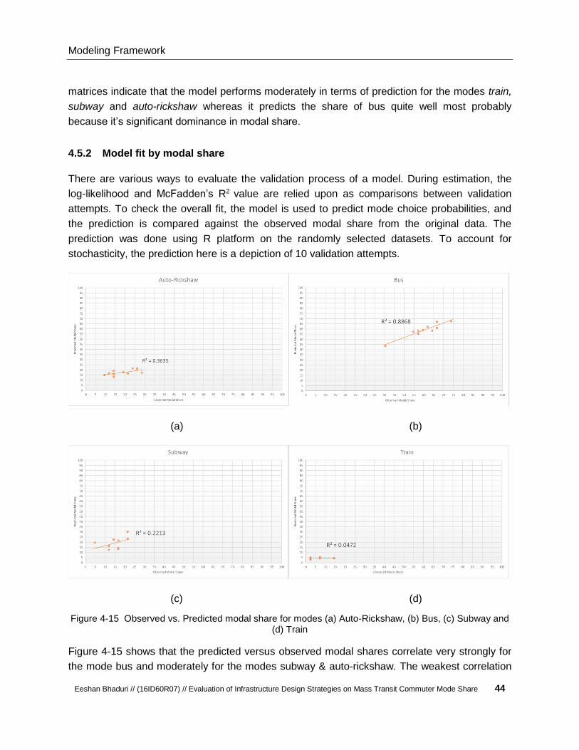
Modeling Framework
Eeshan Bhaduri // (16ID60R07) // Evaluation of Infrastructure Design Strategies on Mass Transit Commuter Mode Share 44
matrices indicate that the model performs moderately in terms of prediction for the modes train,
subway and auto-rickshaw whereas it predicts the share of bus quite well most probably
because it’s significant dominance in modal share.
4.5.2 Model fit by modal share
There are various ways to evaluate the validation process of a model. During estimation, the
log-likelihood and McFadden’s R2 value are relied upon as comparisons between validation
attempts. To check the overall fit, the model is used to predict mode choice probabilities, and
the prediction is compared against the observed modal share from the original data. The
prediction was done using R platform on the randomly selected datasets. To account for
stochasticity, the prediction here is a depiction of 10 validation attempts.
(a) (b)
(c) (d)
Figure 4-15 Observed vs. Predicted modal share for modes (a) Auto-Rickshaw, (b) Bus, (c) Subway and (d) Train
Figure 4-15 shows that the predicted versus observed modal shares correlate very strongly for
the mode bus and moderately for the modes subway & auto-rickshaw. The weakest correlation

Modeling Framework
Eeshan Bhaduri // (16ID60R07) // Evaluation of Infrastructure Design Strategies on Mass Transit Commuter Mode Share 45
belongs to the mode train. However, it should be kept in mind that the mode train has the
smallest number of trip records, only going up to 13 trips that too only in one corridor.
4.5.3 Model fit by trip length
The number of trips per mode per distance is aggregated in 5 km distance brackets, up to
maximum 25 km. The predicted modal shares are graphed against the observed modal shares.
Figure 4-16 Distribution of modal share by trip length (observed vs predicted)
The Figure 4-16 indicates that the predicted modal shares grossly follow the overall pattern of
the observed modal shares, especially for shorter distances and for all the modes. The pattern
is not so closely matched at longer distances specifically between the modes subway and train
because there are very few actual trips made at such distances. That is why most of the train
trips are mis-classified as subway trips. It should be taken into consideration that most trips are
short to medium-distance bus trips, and the model captures that behavior well.

Scenario Analysis
Eeshan Bhaduri // (16ID60R07) // Evaluation of Infrastructure Design Strategies on Mass Transit Commuter Mode Share 46
Chapter 5 - Scenario Analysis
The major objective of this thesis is to assess the impact of different policy interventions in
public transit improvement on commuter mode share. For this assessment, a commuter mode
choice model was built based on field survey as described in Chapter Chapter 4 - above. This
model was then applied to different scenarios of the policy interventions. The results of this
application of the model to the scenarios are described in this chapter.
Figure 5-1 Study area (hatched) & network (existing & proposed) map of city of Kolkata Metropolitan area
The transportation network of Kolkata is literally a labyrinth which is quite apparent from the
Figure removed due to possible copyright infringements

List of References
Eeshan Bhaduri // (16ID60R07) // Evaluation of Infrastructure Design Strategies on Mass Transit Commuter Mode Share 47
Figure 5-1above. At the same time significant portion of the transit corridors are overlapping in
nature making the network far from being optimized. In this chapter the impact of different transit
improvement policies has been analysed. It can give a new direction instead of inducing a new
transport corridor or a new mode every time to solve the age old ‘congestion’ problem.

Scenario Analysis
Eeshan Bhaduri // (16ID60R07) // Evaluation of Infrastructure Design Strategies on Mass Transit Commuter Mode Share 48
5.1 Scenario development
5.1.1 Field study
To understand the operational behavior of different modes along the corridor various mode
related characteristics were observed during the field survey, conducted in the same period as
the perception survey. Similarly, these data-points were collected in three phases of the day –
two peak periods in morning and evening and afternoon off-peak period. The available datasets
are as followed:
Class I – Mode related characteristics
• Corridor travel time
• Frequency of signalized intersection
• Waiting time (with & without signal)
Class II – Mode and Traveler related characteristic
• Demand of the mode (No. of passengers boarding and/or alighting)
• Vehicular occupancy and/or comfortable occupancy (depends on vehicle type)
5.2 Data analysis
5.2.1 Analysis of corridor A - Tollygunge to Kalighat metro station corridor
Analysis I – No. of passengers vs. Stops
(a) (b)

Scenario Analysis
Eeshan Bhaduri // (16ID60R07) // Evaluation of Infrastructure Design Strategies on Mass Transit Commuter Mode Share 49
(c)
Figure 5-2 Passenger demand vs. Stops (a) morning peak, (b) evening peak and (c) afternoon off-peak
It can be clearly observed from Figure 5-2 above that passenger demand is not constant across
all the stops, in fact there are huge gap in the demand for different stops. This situation probably
occurs because of very closely spaced stops (3.6 stops on average per km on this corridor).
Scenario intervention(s): As we can find sudden peaks in the graph we can merge other stops
in the vicinity based on the average walking speed or skip-stop service can also be introduced
to avoid pressure during peak hours. The major stops in terms of passenger demand found out
to be: (1) Tollygunge, (2) Anwar Shah connector, (3) Tollygunge railway station, (4) Mudiali, and
(5) Kalighat metro station.
Analysis II – Average vehicular speed vs. Corridor
(a) (b)

Scenario Analysis
Eeshan Bhaduri // (16ID60R07) // Evaluation of Infrastructure Design Strategies on Mass Transit Commuter Mode Share 50
(c)
Figure 5-3 Average speed (different modes) vs. Stops (a) morning peak, (b) evening peak and (c) afternoon off-peak
It can be inferred from Figure 5-3 above that average vehicular speed fluctuates along the
corridor with sudden peaks making it prone to accidents as well as it causes schedule deviation
rendering to unreliable service. This variation is also a result of competition between different
modes as buses waits intentionally for longer period in a stop to get more passengers which
consequently causes delay and congestion. Moreover, it helps to determine major stops for
skip-stop operation.
Scenario intervention(s): Sudden fluctuation of vehicular speed can be resolved through
optimized station planning and location (avoid major intersection) when skip stop operation or
merging procedure is involved for public transits.
Analysis III – Average travel time vs. Time of day
Figure 5-4 Average total travel time vs. Time of day

Scenario Analysis
Eeshan Bhaduri // (16ID60R07) // Evaluation of Infrastructure Design Strategies on Mass Transit Commuter Mode Share 51
It can be seen in Figure 5-4 above that travel time along the corridor for all types of mode is
higher during peak hours which is in line with general intuition. Simultaneously travel time
difference between auto-rickshaw and bus was not found to be significant which is quite
practical considering most of the arterial streets in Kolkata are overly saturated. It can also be
observed that the travel time for private buses are significantly higher than other type of buses
which is probably due to absence of strict traffic laws and their own unruly traffic behavior.
Scenario intervention(s): The capacity of the streets can be increased through different
options like removal of auto-rickshaw or adding a bus only lane (or a reversible contraflow lane)
which facilitates the use of public transit by overall improvement of vehicular speed and
subsequently travel time.
Analysis IV – Average waiting time vs. Time of day
Figure 5-5 Average waiting time vs. Time of day
Figure 5-5 above shows that waiting time, with and without signal combined, along the corridor
for all types of mode is higher during morning peak hours. This is probably because of
intentional waiting time to capture more passengers in stops especially for private buses and
auto-rickshaw which invariably causes congestion for full length of the section whereas the
trend is opposite in evening peak as expected.
Scenario intervention(s): The waiting time in the stops have a direct relation with the bus stop
capacity and queuing effect on the streets which in turn affects the reliability of the service.

Scenario Analysis
Eeshan Bhaduri // (16ID60R07) // Evaluation of Infrastructure Design Strategies on Mass Transit Commuter Mode Share 52
Analysis V – Average vehicle occupancy(crowdedness) vs. Time of day
Figure 5-6 Average vehicle (comfortable) occupancy vs. Time of day
Average comfortable vehicle occupancy is calculated by adding all the no. of people could stand
comfortably with no. of seats in the vehicle to consider variation in carrying capacity of different
type of vehicle. Figure 5-6above suggests that even for the peak period the occupancy level of
buses is lower than it’s carrying capacity which shows people’s choice of other faster mode like
subway for travel time saving as well as inherent cause like high no. of overlapping routes
running on the corridor. In case of auto-rickshaw the different demand curve does not
essentially shows inclination of people to that mode rather those modes do not ply without being
fully occupied which is reflected in high waiting time Figure 5-5.
Scenario intervention(s): Bus schedule and service frequencies should be thoroughly planned
out to cater to the peak hour demand as well as off-peak efficiently enough.
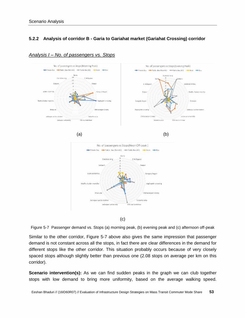
Scenario Analysis
Eeshan Bhaduri // (16ID60R07) // Evaluation of Infrastructure Design Strategies on Mass Transit Commuter Mode Share 53
5.2.2 Analysis of corridor B - Garia to Gariahat market (Gariahat Crossing) corridor
Analysis I – No. of passengers vs. Stops
(a) (b)
(c)
Figure 5-7 Passenger demand vs. Stops (a) morning peak, (b) evening peak and (c) afternoon off-peak
Similar to the other corridor, Figure 5-7 above also gives the same impression that passenger
demand is not constant across all the stops, in fact there are clear differences in the demand for
different stops like the other corridor. This situation probably occurs because of very closely
spaced stops although slightly better than previous one (2.08 stops on average per km on this
corridor).
Scenario intervention(s): As we can find sudden peaks in the graph we can club together
stops with low demand to bring more uniformity, based on the average walking speed.
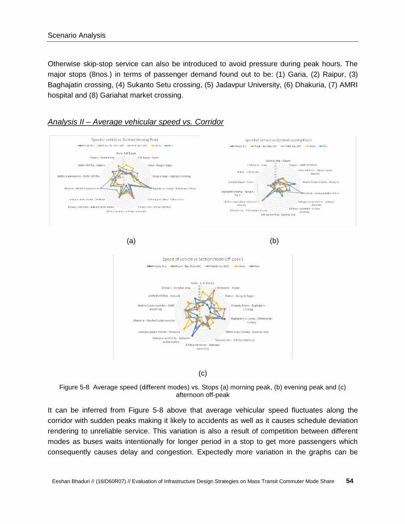
Scenario Analysis
Eeshan Bhaduri // (16ID60R07) // Evaluation of Infrastructure Design Strategies on Mass Transit Commuter Mode Share 54
Otherwise skip-stop service can also be introduced to avoid pressure during peak hours. The
major stops (8nos.) in terms of passenger demand found out to be: (1) Garia, (2) Raipur, (3)
Baghajatin crossing, (4) Sukanto Setu crossing, (5) Jadavpur University, (6) Dhakuria, (7) AMRI
hospital and (8) Gariahat market crossing.
Analysis II – Average vehicular speed vs. Corridor
(a) (b)
(c)
Figure 5-8 Average speed (different modes) vs. Stops (a) morning peak, (b) evening peak and (c) afternoon off-peak
It can be inferred from Figure 5-8 above that average vehicular speed fluctuates along the
corridor with sudden peaks making it likely to accidents as well as it causes schedule deviation
rendering to unreliable service. This variation is also a result of competition between different
modes as buses waits intentionally for longer period in a stop to get more passengers which
consequently causes delay and congestion. Expectedly more variation in the graphs can be
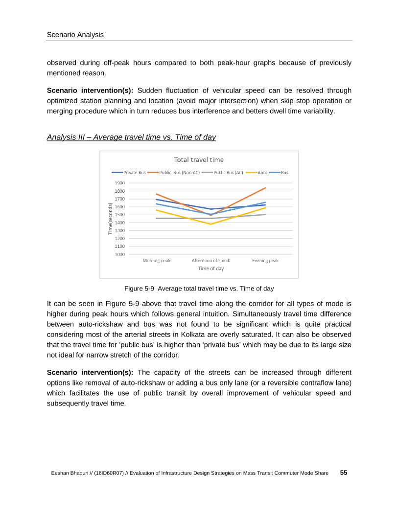
Scenario Analysis
Eeshan Bhaduri // (16ID60R07) // Evaluation of Infrastructure Design Strategies on Mass Transit Commuter Mode Share 55
observed during off-peak hours compared to both peak-hour graphs because of previously
mentioned reason.
Scenario intervention(s): Sudden fluctuation of vehicular speed can be resolved through
optimized station planning and location (avoid major intersection) when skip stop operation or
merging procedure which in turn reduces bus interference and betters dwell time variability.
Analysis III – Average travel time vs. Time of day
Figure 5-9 Average total travel time vs. Time of day
It can be seen in Figure 5-9 above that travel time along the corridor for all types of mode is
higher during peak hours which follows general intuition. Simultaneously travel time difference
between auto-rickshaw and bus was not found to be significant which is quite practical
considering most of the arterial streets in Kolkata are overly saturated. It can also be observed
that the travel time for ‘public bus’ is higher than ‘private bus’ which may be due to its large size
not ideal for narrow stretch of the corridor.
Scenario intervention(s): The capacity of the streets can be increased through different
options like removal of auto-rickshaw or adding a bus only lane (or a reversible contraflow lane)
which facilitates the use of public transit by overall improvement of vehicular speed and
subsequently travel time.

Scenario Analysis
Eeshan Bhaduri // (16ID60R07) // Evaluation of Infrastructure Design Strategies on Mass Transit Commuter Mode Share 56
Analysis IV – Average waiting time vs. Time of day
Figure 5-10 Average waiting time vs. Time of day
Figure 5-10 above shows that waiting time, with and without signal combined, is almost same
for both peak hour span especially for bus mode on average but for auto-rickshaw it’s opposite
probably because of intentional waiting time to capture more passengers in stops during off-
peak and same applies for private buses during morning peak. This invariably causes
congestion for full length of the section as some parts of this corridor is quite narrow (less than 2
lanes).
Scenario intervention(s): The waiting time in the stops have a direct relation with the bus stop
capacity and queuing effect on the streets which in turn affects the reliability of the service.

Scenario Analysis
Eeshan Bhaduri // (16ID60R07) // Evaluation of Infrastructure Design Strategies on Mass Transit Commuter Mode Share 57
Analysis V – Average vehicle occupancy(crowdedness) vs. Time of day
Figure 5-11 Average vehicle (comfortable) occupancy vs. Time of day
Average comfortable vehicle occupancy is calculated by adding all the no. of people could stand
comfortably with no. of seats in the vehicle to consider variation in carrying capacity of different
type of vehicle. Figure 5-11 above suggests that even for the peak period the occupancy level of
buses is lower than it’s carrying capacity which shows people’s choice of other faster mode like
subway for travel time saving as well as inherent cause like high no. of overlapping routes
running on the corridor. In case of auto-rickshaw the different demand curve does not
essentially shows inclination of people to that mode rather those modes do not ply without being
fully occupied which is reflected in high waiting time Figure 5-11.
Scenario intervention(s): Bus schedule and service frequencies should be thoroughly planned
out to cater to the peak hour demand as well as off-peak efficiently enough. New peak hour
services can be introduced in current off-peak slots keeping in mind general working hours in
educational institutions and commercial sector.

Scenario Analysis
Eeshan Bhaduri // (16ID60R07) // Evaluation of Infrastructure Design Strategies on Mass Transit Commuter Mode Share 58
5.3 Transit capacity and speed calculation
To build up different scenarios and to find out which variables could be changed to alter the
travel speed a detailed literature study was done which resulted in estimation of transit capacity
and speed in two study corridors separately based on the methods published in the reports by
Transportation Research Board. (Kittelson & Associates, Inc.; Parsons Brinckerhoff; KFH
Group, Inc; Texas A&M Transportation Institute; ARUP, 2013)
5.3.1 Estimation of existing bus lane capacity
Step 1- Defining facility
i. 2-way couplet
ii. towards downtown area
Step 2- Calculation of bus stop demand data
i. Mean Dwell time = Observed from field study
ii. Dwell time variability (Cv ) = Observed from field study
iii. Failure rate = 15-30% (can be computed)
iv. Passenger demand peak hour factor(PHF) = (boarding + alighting passengers in peak
hour) / (4 x Passenger demand during peak 15 mins)
Step 3- Calculation of bus stop location data
I. Positions relative to road way = Off-line (no curb extension present so bus pulls out of
travel lane to serve a stop)
II. Positions relative to intersection = far-side (located immediately after intersection)
III. Bus stop design type = Linear
IV. Number of Loading area = 1 for each stop
V. Bus facility type = type 2 bus lane (allows bus to move adjacent lane to move around
other vehicles using that lane)
VI. Traffic signal timing = g/C ratio (should be gathered from literature/ secondary source)
VII. Traffic volume (should be gathered from literature/ secondary source)
VIII. Curb lane traffic volume (veh/hr)
IX. Left turning traffic volume & capacity (veh/hr)
X. Parallel Pedestrian crossing volume conflicting with left-turning traffic
XI. Setting a design bus stop failure rate and
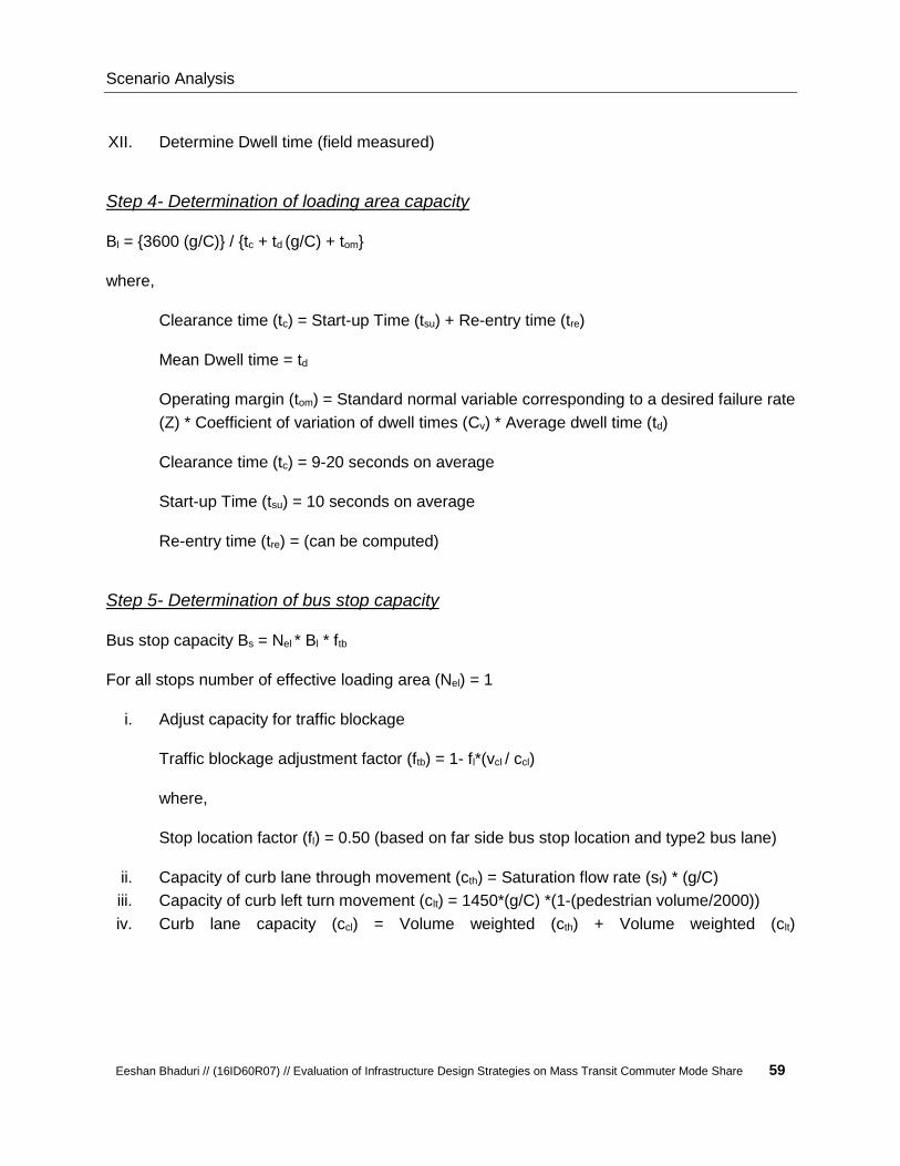
Scenario Analysis
Eeshan Bhaduri // (16ID60R07) // Evaluation of Infrastructure Design Strategies on Mass Transit Commuter Mode Share 59
XII. Determine Dwell time (field measured)
Step 4- Determination of loading area capacity
Bl = {3600 (g/C)} / {tc + td (g/C) + tom}
where,
Clearance time (tc) = Start-up Time (tsu) + Re-entry time (tre)
Mean Dwell time = td
Operating margin (tom) = Standard normal variable corresponding to a desired failure rate
(Z) * Coefficient of variation of dwell times (Cv) * Average dwell time (td)
Clearance time (tc) = 9-20 seconds on average
Start-up Time (tsu) = 10 seconds on average
Re-entry time (tre) = (can be computed)
Step 5- Determination of bus stop capacity
Bus stop capacity Bs = Nel * Bl * ftb
For all stops number of effective loading area (Nel) = 1
i. Adjust capacity for traffic blockage
Traffic blockage adjustment factor (ftb) = 1- fl*(vcl / ccl)
where,
Stop location factor (fl) = 0.50 (based on far side bus stop location and type2 bus lane)
ii. Capacity of curb lane through movement (cth) = Saturation flow rate (sf) * (g/C)
iii. Capacity of curb left turn movement (clt) = 1450*(g/C) *(1-(pedestrian volume/2000))
iv. Curb lane capacity (ccl) = Volume weighted (cth) + Volume weighted (clt)

Scenario Analysis
Eeshan Bhaduri // (16ID60R07) // Evaluation of Infrastructure Design Strategies on Mass Transit Commuter Mode Share 60
5.3.2 Estimation of existing bus lane speed
Step 1- Defining facility
i. 2-way couplet
ii. towards downtown area
Step 2- Calculation of bus stop demand data
i. average stop spacing = stops/Km in each direction (should be field observed)
ii. average dwell time = (should be field observed)
iii. scheduled number of buses at critical stop = (should be field observed)
iv. traffic signal timing and phasing = (should be field observed)
v. traffic interference = signals/Km in each direction
Step 3- Determination of section maximum capacity
It should be the input of the section capacity determined in section 5.3.1 above.
Step 4- Determination of base bus running time rate
i. calculate unimpeded bus running time rate
travel time rate a bus would experience if it could travel along the facility without
traffic signal or traffic delays
tu = { trs + Ns ( tdt + tacc + tdec + tsta )} / 60
where,
unimpeded running time rate = (tu)
time spent at running speed (trs) = Lrs / (cf * vrun)
Distance travelled at running speed per Km (Lrs) = Lmk – Ns Lad
distance travelled at less than running speed
(Lad) = 0.5*a*(tacc)2+0.5*d*(tdec)2+ Lsta
Acceleration time (tacc) = (cf * vrun) / a

Scenario Analysis
Eeshan Bhaduri // (16ID60R07) // Evaluation of Infrastructure Design Strategies on Mass Transit Commuter Mode Share 61
Deceleration time (tdec) = (cf * vrun) / d
Bus running speed on facility = (vrun)
Conversion factor = cf
time required to travel through station (tsta) = Lsta / (1/ cf*vst - 1/ cf*vrun)
ii. calculate additional running time losses (tl)
Running time losses based on type of traffic.
iii. calculate base bus running time rate
tr = tu + tl
Step 5- Adjustment for bus congestion
i. bus v/c = Scheduled no. of Bus in per hour / Max capacity of street
ii. bus-bus interference factor(fbb)
Step 6- Determination of average section speed
i. No adjustment for no skip-stop (fsp) = 1
ii. For skip-stop operation = 0.87 (based on traffic volume)
Step 7- Determination of average section speed
iii. Section running time rate(ts) = tr / fbb * fsp
iv. Average Section speed (Ss) = 60/ ts
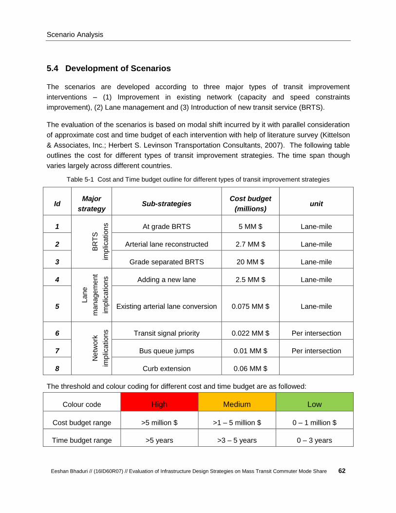
Scenario Analysis
Eeshan Bhaduri // (16ID60R07) // Evaluation of Infrastructure Design Strategies on Mass Transit Commuter Mode Share 62
5.4 Development of Scenarios
The scenarios are developed according to three major types of transit improvement
interventions – (1) Improvement in existing network (capacity and speed constraints
improvement), (2) Lane management and (3) Introduction of new transit service (BRTS).
The evaluation of the scenarios is based on modal shift incurred by it with parallel consideration
of approximate cost and time budget of each intervention with help of literature survey (Kittelson
& Associates, Inc.; Herbert S. Levinson Transportation Consultants, 2007). The following table
outlines the cost for different types of transit improvement strategies. The time span though
varies largely across different countries.
Table 5-1 Cost and Time budget outline for different types of transit improvement strategies
Id Major
strategy Sub-strategies
Cost budget
(millions) unit
1
BR
TS
imp
lica
tion
s
At grade BRTS 5 MM $ Lane-mile
2 Arterial lane reconstructed 2.7 MM $ Lane-mile
3 Grade separated BRTS 20 MM $ Lane-mile
4
Lane
ma
na
ge
me
nt
imp
lica
tion
s
Adding a new lane 2.5 MM $ Lane-mile
5 Existing arterial lane conversion 0.075 MM $ Lane-mile
6
Ne
twork
imp
lica
tion
s
Transit signal priority 0.022 MM $ Per intersection
7 Bus queue jumps 0.01 MM $ Per intersection
8 Curb extension 0.06 MM $
The threshold and colour coding for different cost and time budget are as followed:
Colour code High Medium Low
Cost budget range >5 million $ >1 – 5 million $ 0 – 1 million $
Time budget range >5 years >3 – 5 years 0 – 3 years
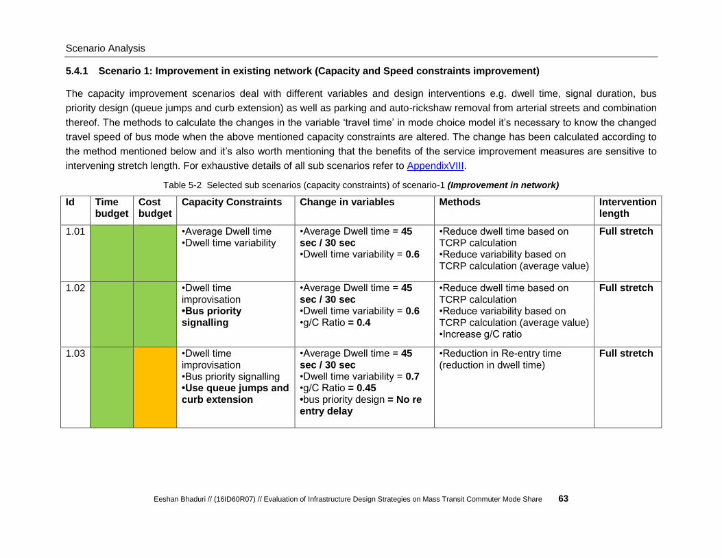
Scenario Analysis
Eeshan Bhaduri // (16ID60R07) // Evaluation of Infrastructure Design Strategies on Mass Transit Commuter Mode Share 63
5.4.1 Scenario 1: Improvement in existing network (Capacity and Speed constraints improvement)
The capacity improvement scenarios deal with different variables and design interventions e.g. dwell time, signal duration, bus
priority design (queue jumps and curb extension) as well as parking and auto-rickshaw removal from arterial streets and combination
thereof. The methods to calculate the changes in the variable ‘travel time’ in mode choice model it’s necessary to know the changed
travel speed of bus mode when the above mentioned capacity constraints are altered. The change has been calculated according to
the method mentioned below and it’s also worth mentioning that the benefits of the service improvement measures are sensitive to
intervening stretch length. For exhaustive details of all sub scenarios refer to AppendixVIII.
Table 5-2 Selected sub scenarios (capacity constraints) of scenario-1 (Improvement in network)
Id Time budget
Cost budget
Capacity Constraints Change in variables Methods Intervention length
1.01 •Average Dwell time •Dwell time variability
•Average Dwell time = 45 sec / 30 sec •Dwell time variability = 0.6
•Reduce dwell time based on TCRP calculation •Reduce variability based on TCRP calculation (average value)
Full stretch
1.02 •Dwell time improvisation •Bus priority signalling
•Average Dwell time = 45 sec / 30 sec •Dwell time variability = 0.6 •g/C Ratio = 0.4
•Reduce dwell time based on TCRP calculation •Reduce variability based on TCRP calculation (average value) •Increase g/C ratio
Full stretch
1.03 •Dwell time improvisation •Bus priority signalling •Use queue jumps and curb extension
•Average Dwell time = 45 sec / 30 sec •Dwell time variability = 0.7 •g/C Ratio = 0.45 •bus priority design = No re entry delay
•Reduction in Re-entry time (reduction in dwell time)
Full stretch

Scenario Analysis
Eeshan Bhaduri // (16ID60R07) // Evaluation of Infrastructure Design Strategies on Mass Transit Commuter Mode Share 64
The scenarios related with improvement of speed constraints considers variables and design interventions e.g. stop spacing / stop
density, skip stop operation, bus schedule (frequency of buses at critical stop at peak hour) etc. and combination thereof. The
changes have been calculated based on the methods mentioned below and in all the cases the measure has been applied to full
stretch length. For exhaustive details of all sub scenarios refer to AppendixIX.
Table 5-3 Selected sub scenarios (speed constraints) of scenario-1 (Improvement in network)
Id Time budget
Cost budget
Speed Constraints Change in variables Methods Intervention length
1.08 •Average stop spacing •Average stop spacing = Increased
•Merge less popular stops Full stretch
1.09 •Average stop spacing •Introduce skip-stop operation
•Average stop spacing = Increased •Skip stop factor =0.87
•Merge less popular stops •Add skip stop operation calculation from TCRP report
Full stretch
1.10 •Average stop spacing •Schedule of Buses at critical stop
•Average stop spacing = Increased •No. of bus/hr at critical stop = 20% overlap removed
•Merge less popular stops •Reduce no. of buses with overlapping route
Full stretch

Scenario Analysis
Eeshan Bhaduri // (16ID60R07) // Evaluation of Infrastructure Design Strategies on Mass Transit Commuter Mode Share 65
5.4.2 Scenario 2: Improvement in lane management
Lane management is second scenario type which deals with the variables and design interventions where both speed and capacity
constraints are improved upon related to lane specification. At the same time measures also considers parking and auto-rickshaw
removal from arterial streets for scenario development. For exhaustive details of all sub scenarios refer to AppendixX.
Table 5-4 Selected sub scenarios of scenario-2 (Improvement in lane management)
Id Time budget
Cost budget
Speed Constraints
Capacity Constraints
Change in variables Methods Intervention length
2.04 •Average stop spacing •Schedule of Buses at critical stop •Introduce skip-stop operation
•Dedicated bus lane from existing road width in extended peak hours span •Bus priority signalling
•Average stop spacing = Increased •No. of bus/hr at critical stop = Changed •Skip stop factor =0.87 •saturation flow = decreased •curb lane volume = bus only lane •new peak hour slots = 8-11, 12-14, 15-17, 18-22 •g/C Ratio = 0.4
•Merge less popular stops •Reduce no. of buses with overlapping route •car & auto rickshaw volume reduced •Change saturation flow based on available road width •Change peak hour variable
Selected stretch
2.16 •Average stop spacing •Schedule of Buses at critical stop •Introduce skip-stop operation
•Introducing contraflow car lane in extended peak hours span (NO car allowed on peak direction) •Removal of Auto-Rickshaw from arterial street •Bus priority signalling
•Average stop spacing = Increased •No. of bus/hr at critical stop = Changed. •Skip stop factor =0.87 •saturation flow = same •curb lane volume = decreased by 60% •new peak hour slots = 8-11, 12-14, 15-17, 18-22 •g/C Ratio = 0.4
•Merge less popular stops •Reduce no. of buses with overlapping route •car & auto rickshaw volume reduced •Change saturation flow based on available road width •Change peak hour variable •g/C Ratio = 0.4
Selected stretch
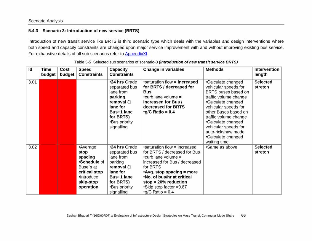
Scenario Analysis
Eeshan Bhaduri // (16ID60R07) // Evaluation of Infrastructure Design Strategies on Mass Transit Commuter Mode Share 66
5.4.3 Scenario 3: Introduction of new service (BRTS)
Introduction of new transit service like BRTS is third scenario type which deals with the variables and design interventions where
both speed and capacity constraints are changed upon major service improvement with and without improving existing bus service.
For exhaustive details of all sub scenarios refer to AppendixXI.
Table 5-5 Selected sub scenarios of scenario-3 (Introduction of new transit service BRTS)
Id Time budget
Cost budget
Speed Constraints
Capacity Constraints
Change in variables Methods Intervention length
3.01 •24 hrs Grade separated bus lane from parking removal (1 lane for Bus+1 lane for BRTS) •Bus priority signalling
•saturation flow = increased for BRTS / decreased for Bus •curb lane volume = increased for Bus / decreased for BRTS •g/C Ratio = 0.4
•Calculate changed vehicular speeds for BRTS buses based on traffic volume change •Calculate changed vehicular speeds for other Buses based on traffic volume change •Calculate changed vehicular speeds for auto-rickshaw mode •Calculate changed waiting time
Selected stretch
3.02 •Average stop spacing •Schedule of Buse`s at critical stop •Introduce skip-stop operation
•24 hrs Grade separated bus lane from parking removal (1 lane for Bus+1 lane for BRTS) •Bus priority signalling
•saturation flow = increased for BRTS / decreased for Bus •curb lane volume = increased for Bus / decreased for BRTS •Avg. stop spacing = more •No. of bus/hr at critical stop = 20% reduction •Skip stop factor =0.87 •g/C Ratio = 0.4
•Same as above Selected stretch
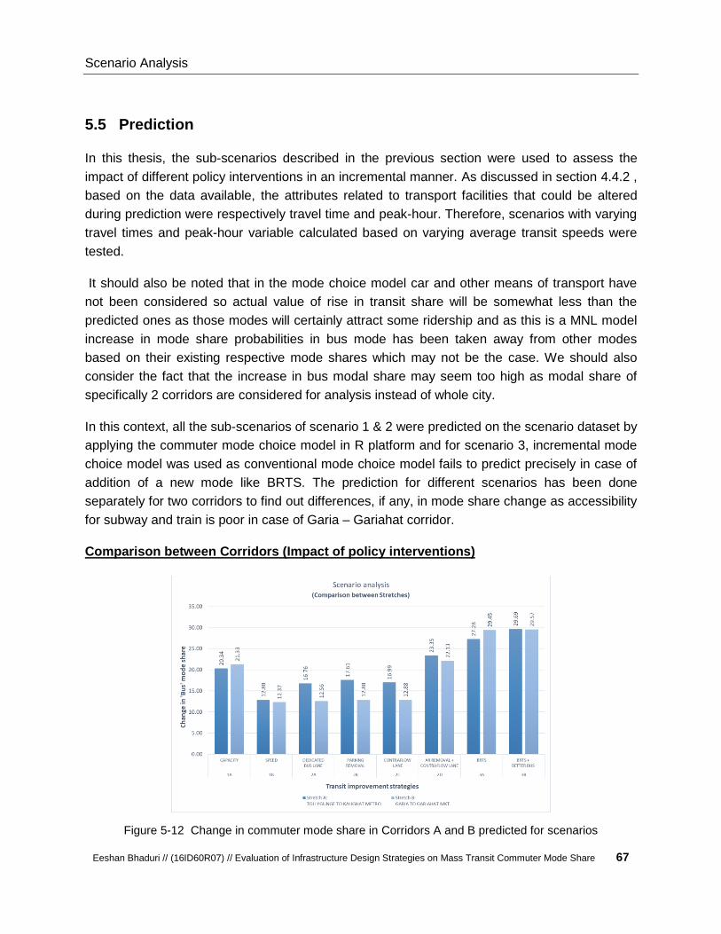
Scenario Analysis
Eeshan Bhaduri // (16ID60R07) // Evaluation of Infrastructure Design Strategies on Mass Transit Commuter Mode Share 67
5.5 Prediction
In this thesis, the sub-scenarios described in the previous section were used to assess the
impact of different policy interventions in an incremental manner. As discussed in section 4.4.2 ,
based on the data available, the attributes related to transport facilities that could be altered
during prediction were respectively travel time and peak-hour. Therefore, scenarios with varying
travel times and peak-hour variable calculated based on varying average transit speeds were
tested.
It should also be noted that in the mode choice model car and other means of transport have
not been considered so actual value of rise in transit share will be somewhat less than the
predicted ones as those modes will certainly attract some ridership and as this is a MNL model
increase in mode share probabilities in bus mode has been taken away from other modes
based on their existing respective mode shares which may not be the case. We should also
consider the fact that the increase in bus modal share may seem too high as modal share of
specifically 2 corridors are considered for analysis instead of whole city.
In this context, all the sub-scenarios of scenario 1 & 2 were predicted on the scenario dataset by
applying the commuter mode choice model in R platform and for scenario 3, incremental mode
choice model was used as conventional mode choice model fails to predict precisely in case of
addition of a new mode like BRTS. The prediction for different scenarios has been done
separately for two corridors to find out differences, if any, in mode share change as accessibility
for subway and train is poor in case of Garia – Gariahat corridor.
Comparison between Corridors (Impact of policy interventions)
Figure 5-12 Change in commuter mode share in Corridors A and B predicted for scenarios
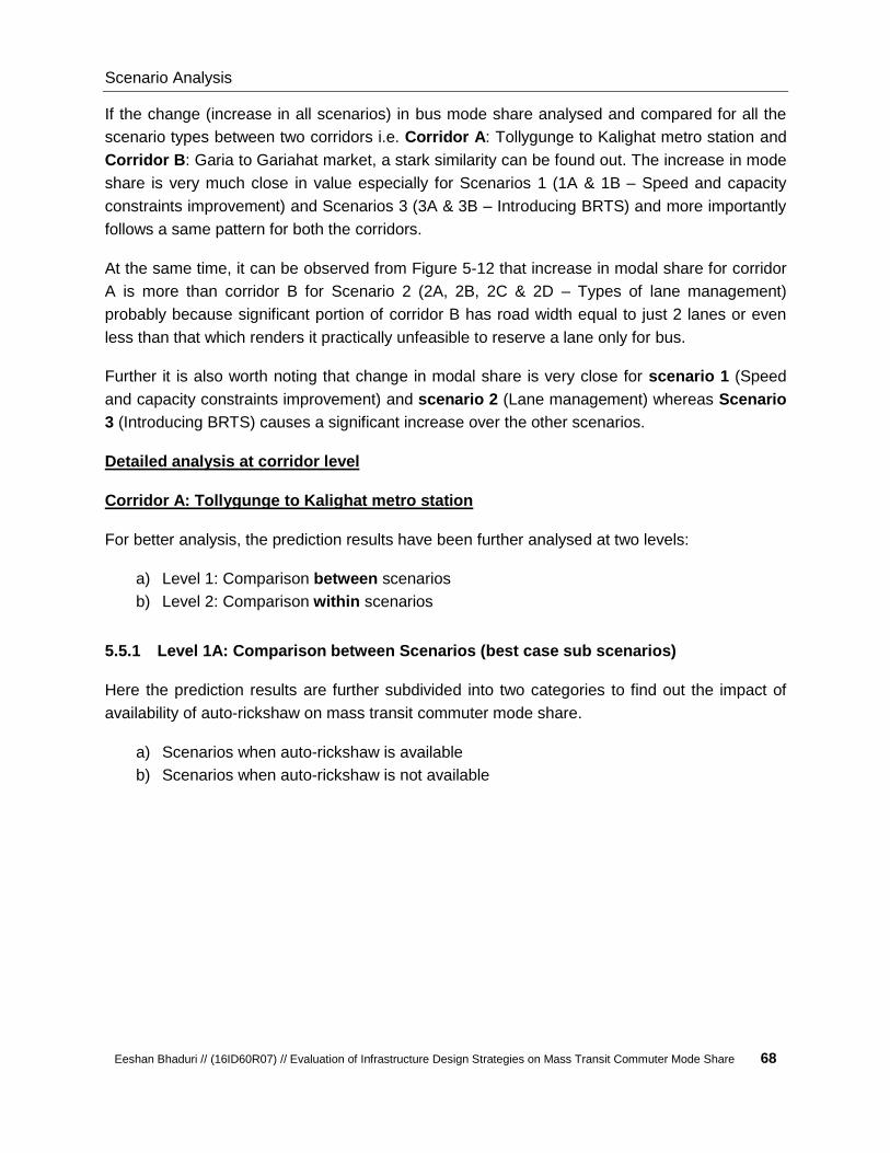
Scenario Analysis
Eeshan Bhaduri // (16ID60R07) // Evaluation of Infrastructure Design Strategies on Mass Transit Commuter Mode Share 68
If the change (increase in all scenarios) in bus mode share analysed and compared for all the
scenario types between two corridors i.e. Corridor A: Tollygunge to Kalighat metro station and
Corridor B: Garia to Gariahat market, a stark similarity can be found out. The increase in mode
share is very much close in value especially for Scenarios 1 (1A & 1B – Speed and capacity
constraints improvement) and Scenarios 3 (3A & 3B – Introducing BRTS) and more importantly
follows a same pattern for both the corridors.
At the same time, it can be observed from Figure 5-12 that increase in modal share for corridor
A is more than corridor B for Scenario 2 (2A, 2B, 2C & 2D – Types of lane management)
probably because significant portion of corridor B has road width equal to just 2 lanes or even
less than that which renders it practically unfeasible to reserve a lane only for bus.
Further it is also worth noting that change in modal share is very close for scenario 1 (Speed
and capacity constraints improvement) and scenario 2 (Lane management) whereas Scenario
3 (Introducing BRTS) causes a significant increase over the other scenarios.
Detailed analysis at corridor level
Corridor A: Tollygunge to Kalighat metro station
For better analysis, the prediction results have been further analysed at two levels:
a) Level 1: Comparison between scenarios
b) Level 2: Comparison within scenarios
5.5.1 Level 1A: Comparison between Scenarios (best case sub scenarios)
Here the prediction results are further subdivided into two categories to find out the impact of
availability of auto-rickshaw on mass transit commuter mode share.
a) Scenarios when auto-rickshaw is available
b) Scenarios when auto-rickshaw is not available

Scenario Analysis
Eeshan Bhaduri // (16ID60R07) // Evaluation of Infrastructure Design Strategies on Mass Transit Commuter Mode Share 69
(a)
(b)
Figure 5-13 Commuter mode share predicted for scenarios (a) auto-rickshaw available and (b) auto-rickshaw not available
There are two points which can be inferred from above figures – (i) increase in mode choice
probabilities through simple speed & capacity improvement techniques (scenario 1) are almost
equal or even greater than comparatively cost & time intensive lane management techniques
(scenario 2) and (ii) removal of auto-rickshaw increases significantly choice probability for bus
across all the scenarios.

Scenario Analysis
Eeshan Bhaduri // (16ID60R07) // Evaluation of Infrastructure Design Strategies on Mass Transit Commuter Mode Share 70
5.5.2 Level 2A: Comparison within Scenarios
Level 2A.1: Scenario 1 – sub scenarios
Here the prediction results are further subdivided into two categories to find out the impact of
improving various capacity and speed constraints on mass transit commuter mode share.
a) Scenario 1.01 – 1.07 - Scenarios with capacity improvement measures (AppendixVIII)
b) Scenario 1.08 – 1.11 - Scenarios when speed improvement measures ( AppendixIX)
(a)
(b)
Figure 5-14 Change in commuter mode share predicted for scenario level 2.1 (a) above and (b) below
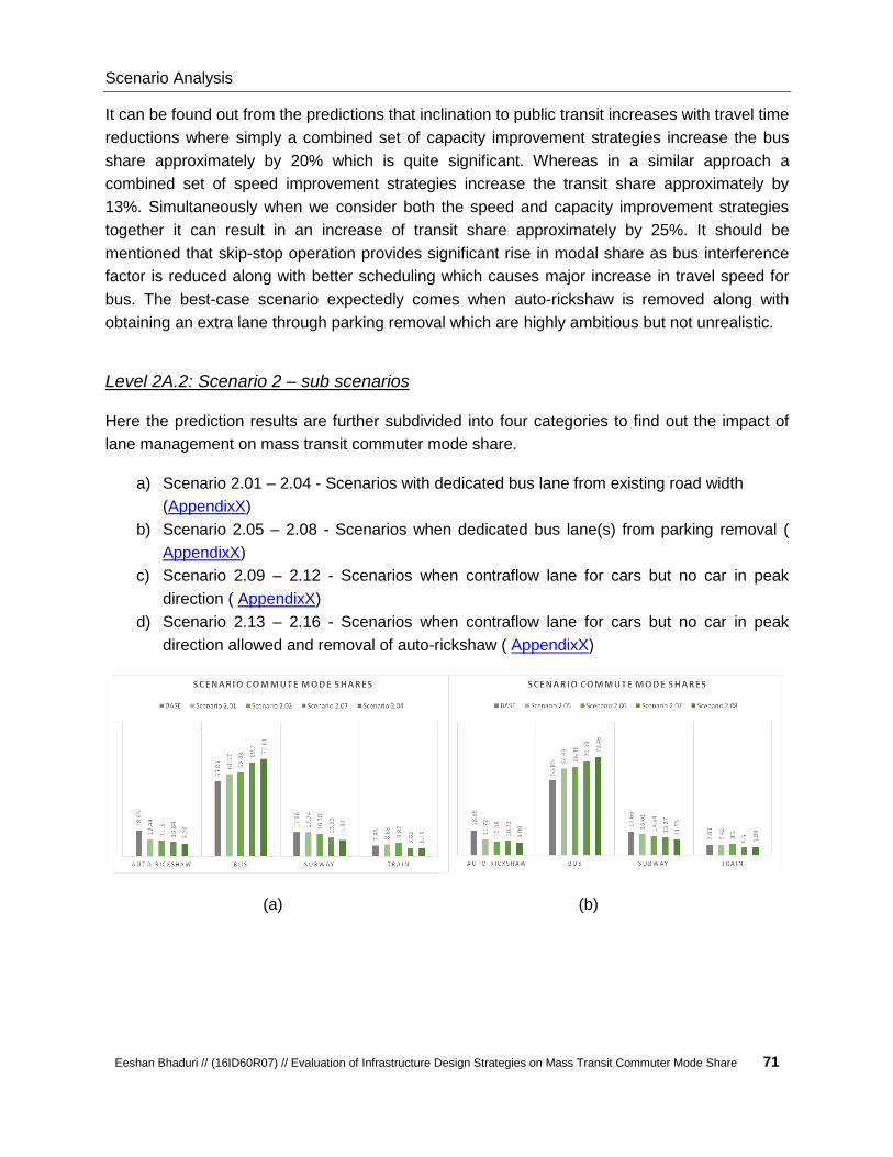
Scenario Analysis
Eeshan Bhaduri // (16ID60R07) // Evaluation of Infrastructure Design Strategies on Mass Transit Commuter Mode Share 71
It can be found out from the predictions that inclination to public transit increases with travel time
reductions where simply a combined set of capacity improvement strategies increase the bus
share approximately by 20% which is quite significant. Whereas in a similar approach a
combined set of speed improvement strategies increase the transit share approximately by
13%. Simultaneously when we consider both the speed and capacity improvement strategies
together it can result in an increase of transit share approximately by 25%. It should be
mentioned that skip-stop operation provides significant rise in modal share as bus interference
factor is reduced along with better scheduling which causes major increase in travel speed for
bus. The best-case scenario expectedly comes when auto-rickshaw is removed along with
obtaining an extra lane through parking removal which are highly ambitious but not unrealistic.
Level 2A.2: Scenario 2 – sub scenarios
Here the prediction results are further subdivided into four categories to find out the impact of
lane management on mass transit commuter mode share.
a) Scenario 2.01 – 2.04 - Scenarios with dedicated bus lane from existing road width
(AppendixX)
b) Scenario 2.05 – 2.08 - Scenarios when dedicated bus lane(s) from parking removal (
AppendixX)
c) Scenario 2.09 – 2.12 - Scenarios when contraflow lane for cars but no car in peak
direction ( AppendixX)
d) Scenario 2.13 – 2.16 - Scenarios when contraflow lane for cars but no car in peak
direction allowed and removal of auto-rickshaw ( AppendixX)
(a) (b)

Scenario Analysis
Eeshan Bhaduri // (16ID60R07) // Evaluation of Infrastructure Design Strategies on Mass Transit Commuter Mode Share 72
(c) (d)
Figure 5-15 Change in commuter mode share predicted for scenario level 2.2 (a) above left, (b) above right, (c) below left and (d) below right
The predictions show that bus modal share expectedly increases with better lane management
strategies. All the sub scenarios clearly show that whenever speed improvement strategies are
coupled with the lane management strategies there is significant rise in transit share.
Introduction of new peak hour services (Scenario 2.02, 2.04, 2.06, 2.08, 2.10, 2.12, 2.14 & 2.16)
during afternoon off peak increase mode share consistently for all sub-scenarios although does
not cause huge increase in transit share when applied without bus priority strategies. It should
still be noted as small increase can also be attributed to the fact that during non-peak hours
people mostly chose bus for travel cost saving. Simultaneously it can be found out that adding
speed improvement measure (Scenario 2.03, 2.05, 2.07, 2.09, 2.11, 2.13, 2.15 & 2.17) makes a
significant impact in increasing mode share for bus consistently. The best-case scenario among
all lane management interventions comes up when car use has been restricted along with
removal of auto-rickshaw from arterial street.
Level 2A.3: Scenario 3 – sub scenarios
Here the prediction results are further subdivided into two categories to find out the impact of
introduction of a new service like Bus rapid transit system (BRTS) on mass transit commuter
mode share.
a) Scenario 3.01 - Scenarios with additional BRTS service, no improvement of existing bus
service ( AppendixXI)
b) Scenario 3.02 - Scenarios with additional BRTS service and speed improvement
measures for existing Bus service ( AppendixXI)
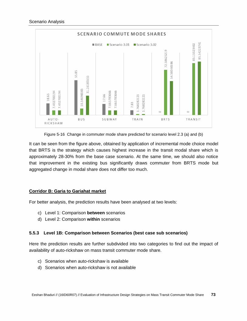
Scenario Analysis
Eeshan Bhaduri // (16ID60R07) // Evaluation of Infrastructure Design Strategies on Mass Transit Commuter Mode Share 73
Figure 5-16 Change in commuter mode share predicted for scenario level 2.3 (a) and (b)
It can be seen from the figure above, obtained by application of incremental mode choice model
that BRTS is the strategy which causes highest increase in the transit modal share which is
approximately 28-30% from the base case scenario. At the same time, we should also notice
that improvement in the existing bus significantly draws commuter from BRTS mode but
aggregated change in modal share does not differ too much.
Corridor B: Garia to Gariahat market
For better analysis, the prediction results have been analysed at two levels:
c) Level 1: Comparison between scenarios
d) Level 2: Comparison within scenarios
5.5.3 Level 1B: Comparison between Scenarios (best case sub scenarios)
Here the prediction results are further subdivided into two categories to find out the impact of
availability of auto-rickshaw on mass transit commuter mode share.
c) Scenarios when auto-rickshaw is available
d) Scenarios when auto-rickshaw is not available
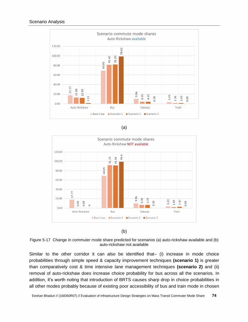
Scenario Analysis
Eeshan Bhaduri // (16ID60R07) // Evaluation of Infrastructure Design Strategies on Mass Transit Commuter Mode Share 74
(a)
(b)
Figure 5-17 Change in commuter mode share predicted for scenarios (a) auto-rickshaw available and (b) auto-rickshaw not available
Similar to the other corridor it can also be identified that– (i) increase in mode choice
probabilities through simple speed & capacity improvement techniques (scenario 1) is greater
than comparatively cost & time intensive lane management techniques (scenario 2) and (ii)
removal of auto-rickshaw does increase choice probability for bus across all the scenarios. In
addition, it’s worth noting that introduction of BRTS causes sharp drop in choice probabilities in
all other modes probably because of existing poor accessibility of bus and train mode in chosen

Scenario Analysis
Eeshan Bhaduri // (16ID60R07) // Evaluation of Infrastructure Design Strategies on Mass Transit Commuter Mode Share 75
corridor (Corridor B) which actually caused initial high modal share for bus and corresponding
low share for all other modes.
5.5.4 Level 2B: Comparison within Scenarios
Level 2B.1: Scenario 1 – sub scenarios
Here the prediction results are further subdivided into two categories to find out the impact of
improving various capacity and speed constraints on mass transit commuter mode share.
a) Scenario 1.01 – 1.07 - Scenarios with capacity improvement measures ( AppendixVIII)
b) Scenario 1.08 – 1.11 - Scenarios when speed improvement measures ( AppendixIX)
(a)

Scenario Analysis
Eeshan Bhaduri // (16ID60R07) // Evaluation of Infrastructure Design Strategies on Mass Transit Commuter Mode Share 76
(b)
Figure 5-18 Change in commuter mode share predicted for scenario level 2.1 (a) above and (b) below
The change in mode choice probabilities follows similar pattern as in other corridor with the
combination of speed and capacity improvement techniques resulting in highest change
(22.70%). It should also be kept in mind that the mode choice probabilities for bus is significantly
higher in this corridor compared to the other mostly due to poor accessibility of other mass
transit modes.
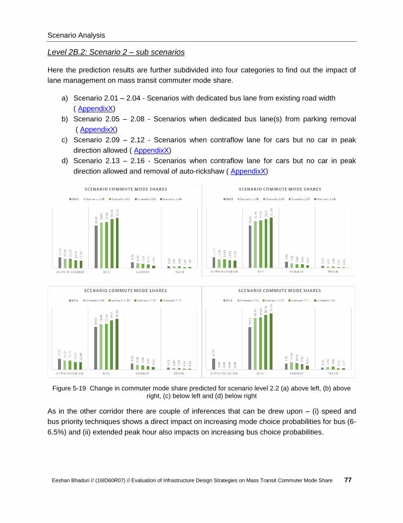
Scenario Analysis
Eeshan Bhaduri // (16ID60R07) // Evaluation of Infrastructure Design Strategies on Mass Transit Commuter Mode Share 77
Level 2B.2: Scenario 2 – sub scenarios
Here the prediction results are further subdivided into four categories to find out the impact of
lane management on mass transit commuter mode share.
a) Scenario 2.01 – 2.04 - Scenarios with dedicated bus lane from existing road width
( AppendixX)
b) Scenario 2.05 – 2.08 - Scenarios when dedicated bus lane(s) from parking removal
( AppendixX)
c) Scenario 2.09 – 2.12 - Scenarios when contraflow lane for cars but no car in peak
direction allowed ( AppendixX)
d) Scenario 2.13 – 2.16 - Scenarios when contraflow lane for cars but no car in peak
direction allowed and removal of auto-rickshaw ( AppendixX)
Figure 5-19 Change in commuter mode share predicted for scenario level 2.2 (a) above left, (b) above right, (c) below left and (d) below right
As in the other corridor there are couple of inferences that can be drew upon – (i) speed and
bus priority techniques shows a direct impact on increasing mode choice probabilities for bus (6-
6.5%) and (ii) extended peak hour also impacts on increasing bus choice probabilities.
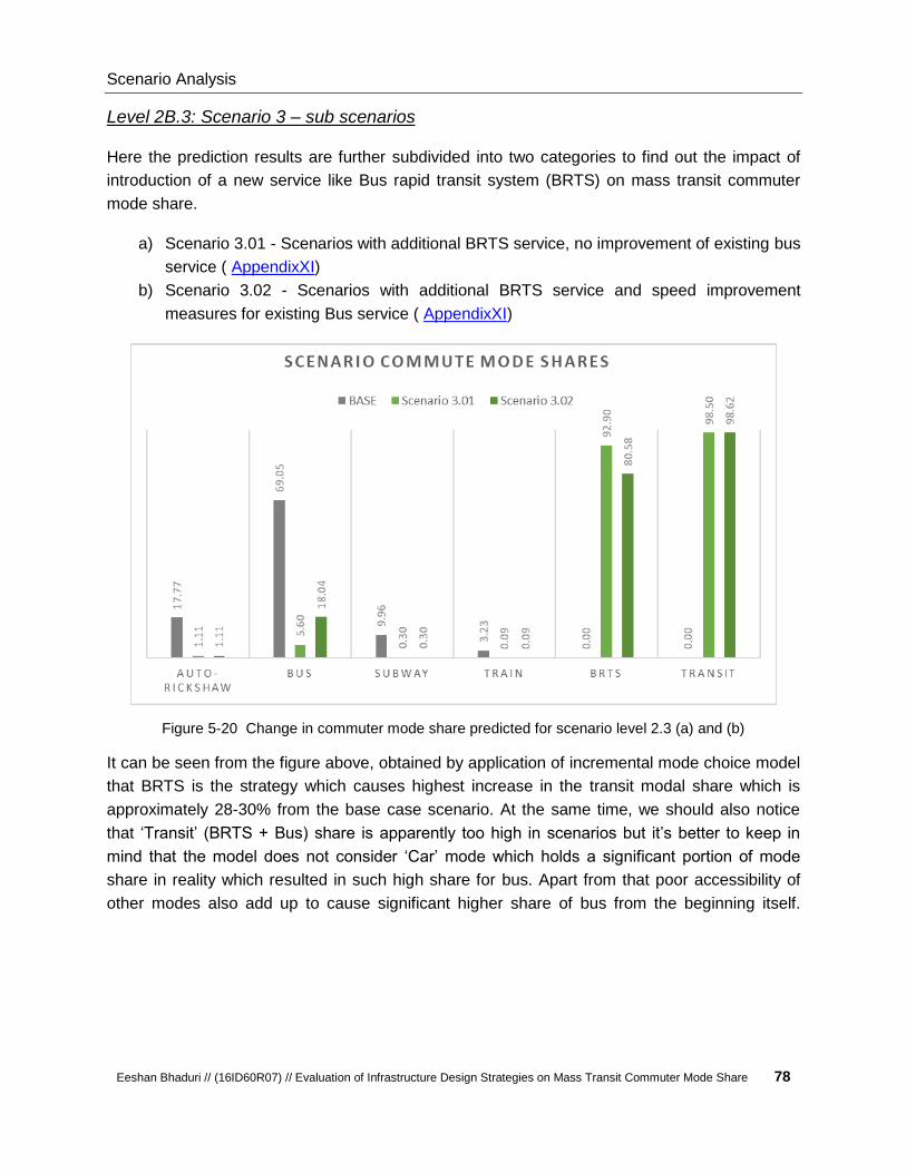
Scenario Analysis
Eeshan Bhaduri // (16ID60R07) // Evaluation of Infrastructure Design Strategies on Mass Transit Commuter Mode Share 78
Level 2B.3: Scenario 3 – sub scenarios
Here the prediction results are further subdivided into two categories to find out the impact of
introduction of a new service like Bus rapid transit system (BRTS) on mass transit commuter
mode share.
a) Scenario 3.01 - Scenarios with additional BRTS service, no improvement of existing bus
service ( AppendixXI)
b) Scenario 3.02 - Scenarios with additional BRTS service and speed improvement
measures for existing Bus service ( AppendixXI)
Figure 5-20 Change in commuter mode share predicted for scenario level 2.3 (a) and (b)
It can be seen from the figure above, obtained by application of incremental mode choice model
that BRTS is the strategy which causes highest increase in the transit modal share which is
approximately 28-30% from the base case scenario. At the same time, we should also notice
that ‘Transit’ (BRTS + Bus) share is apparently too high in scenarios but it’s better to keep in
mind that the model does not consider ‘Car’ mode which holds a significant portion of mode
share in reality which resulted in such high share for bus. Apart from that poor accessibility of
other modes also add up to cause significant higher share of bus from the beginning itself.
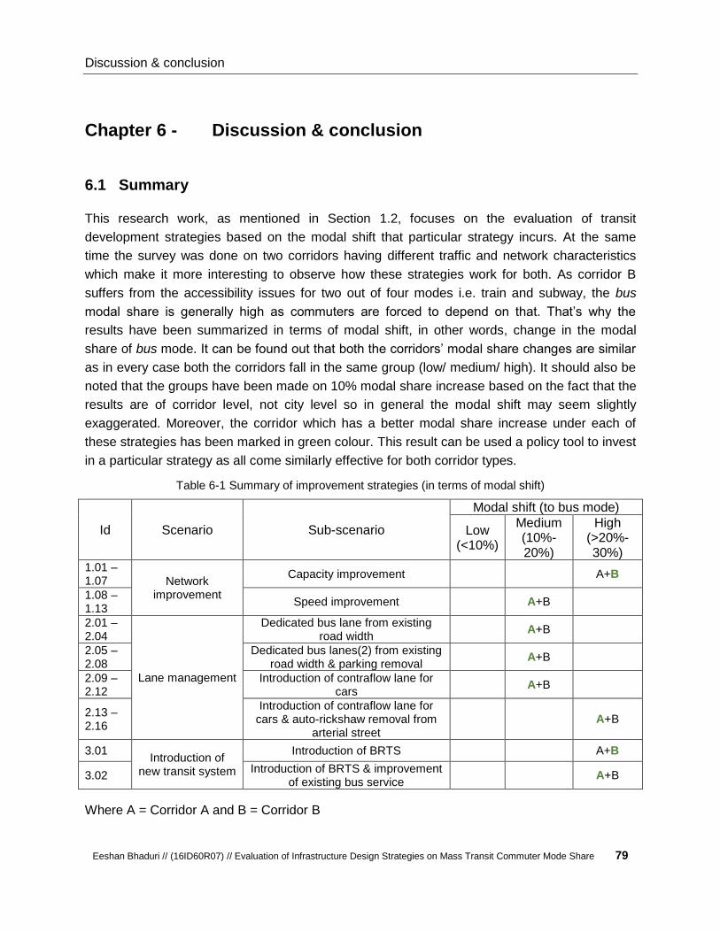
Discussion & conclusion
Eeshan Bhaduri // (16ID60R07) // Evaluation of Infrastructure Design Strategies on Mass Transit Commuter Mode Share 79
Chapter 6 - Discussion & conclusion
6.1 Summary
This research work, as mentioned in Section 1.2, focuses on the evaluation of transit
development strategies based on the modal shift that particular strategy incurs. At the same
time the survey was done on two corridors having different traffic and network characteristics
which make it more interesting to observe how these strategies work for both. As corridor B
suffers from the accessibility issues for two out of four modes i.e. train and subway, the bus
modal share is generally high as commuters are forced to depend on that. That’s why the
results have been summarized in terms of modal shift, in other words, change in the modal
share of bus mode. It can be found out that both the corridors’ modal share changes are similar
as in every case both the corridors fall in the same group (low/ medium/ high). It should also be
noted that the groups have been made on 10% modal share increase based on the fact that the
results are of corridor level, not city level so in general the modal shift may seem slightly
exaggerated. Moreover, the corridor which has a better modal share increase under each of
these strategies has been marked in green colour. This result can be used a policy tool to invest
in a particular strategy as all come similarly effective for both corridor types.
Table 6-1 Summary of improvement strategies (in terms of modal shift)
Id Scenario Sub-scenario
Modal shift (to bus mode)
Low (<10%)
Medium (10%-20%)
High (>20%-30%)
1.01 – 1.07 Network
improvement
Capacity improvement A+B
1.08 – 1.13
Speed improvement A+B
2.01 – 2.04
Lane management
Dedicated bus lane from existing road width
A+B
2.05 – 2.08
Dedicated bus lanes(2) from existing road width & parking removal
A+B
2.09 – 2.12
Introduction of contraflow lane for cars
A+B
2.13 – 2.16
Introduction of contraflow lane for cars & auto-rickshaw removal from
arterial street A+B
3.01 Introduction of
new transit system
Introduction of BRTS A+B
3.02 Introduction of BRTS & improvement
of existing bus service A+B
Where A = Corridor A and B = Corridor B
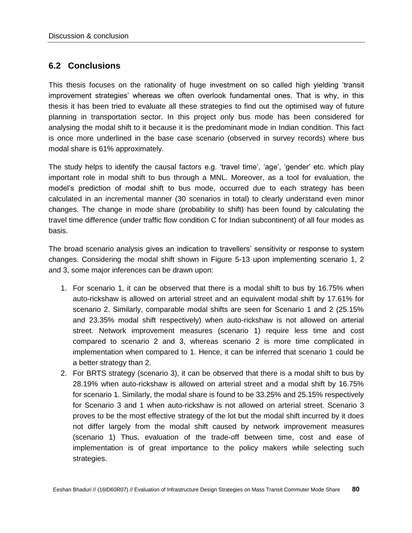
Discussion & conclusion
Eeshan Bhaduri // (16ID60R07) // Evaluation of Infrastructure Design Strategies on Mass Transit Commuter Mode Share 80
6.2 Conclusions
This thesis focuses on the rationality of huge investment on so called high yielding ‘transit
improvement strategies’ whereas we often overlook fundamental ones. That is why, in this
thesis it has been tried to evaluate all these strategies to find out the optimised way of future
planning in transportation sector. In this project only bus mode has been considered for
analysing the modal shift to it because it is the predominant mode in Indian condition. This fact
is once more underlined in the base case scenario (observed in survey records) where bus
modal share is 61% approximately.
The study helps to identify the causal factors e.g. ‘travel time’, ‘age’, ‘gender’ etc. which play
important role in modal shift to bus through a MNL. Moreover, as a tool for evaluation, the
model’s prediction of modal shift to bus mode, occurred due to each strategy has been
calculated in an incremental manner (30 scenarios in total) to clearly understand even minor
changes. The change in mode share (probability to shift) has been found by calculating the
travel time difference (under traffic flow condition C for Indian subcontinent) of all four modes as
basis.
The broad scenario analysis gives an indication to travellers’ sensitivity or response to system
changes. Considering the modal shift shown in Figure 5-13 upon implementing scenario 1, 2
and 3, some major inferences can be drawn upon:
1. For scenario 1, it can be observed that there is a modal shift to bus by 16.75% when
auto-rickshaw is allowed on arterial street and an equivalent modal shift by 17.61% for
scenario 2. Similarly, comparable modal shifts are seen for Scenario 1 and 2 (25.15%
and 23.35% modal shift respectively) when auto-rickshaw is not allowed on arterial
street. Network improvement measures (scenario 1) require less time and cost
compared to scenario 2 and 3, whereas scenario 2 is more time complicated in
implementation when compared to 1. Hence, it can be inferred that scenario 1 could be
a better strategy than 2.
2. For BRTS strategy (scenario 3), it can be observed that there is a modal shift to bus by
28.19% when auto-rickshaw is allowed on arterial street and a modal shift by 16.75%
for scenario 1. Similarly, the modal share is found to be 33.25% and 25.15% respectively
for Scenario 3 and 1 when auto-rickshaw is not allowed on arterial street. Scenario 3
proves to be the most effective strategy of the lot but the modal shift incurred by it does
not differ largely from the modal shift caused by network improvement measures
(scenario 1) Thus, evaluation of the trade-off between time, cost and ease of
implementation is of great importance to the policy makers while selecting such
strategies.
Discussion & conclusion
Eeshan Bhaduri // (16ID60R07) // Evaluation of Infrastructure Design Strategies on Mass Transit Commuter Mode Share 81
3. Auto-rickshaw removal from arterial streets can prove to be more advantageous strategy
in case of scenario 1 compared to scenario 2 and scenario 3 which anyway frees up
exclusive lane (space) for bus. The modal share differences are 8.4%, 5.74% and 5.06%
between situations when auto-rickshaw is available or not respectively for scenario 1, 2
and 3.
At the same time, it can also be pointed out that small dataset size does not always necessarily
plagues the model and even though this model is based on small number of records it performs
average to well in re-estimation and somewhat in validation too. A certain level of confidence on
the model can be built upon based on iterative (10 times in this case) re-estimation exercise as
well as validation attempts can also be done on various aspects to evaluate model performance.
6.3 Recommendations
6.3.1 Policy suggestions for corridor A (Tollygunje to Kalighat Metro Station)
As the traffic characteristics has been already analysed in section 5.2.1 and modal shift shown
in section 5.5.2 acts as an indicator for policy making with respect to corridor A. The policies
that could be formulated are as follows:
1. Use of site specific bus preferential treatments like queue jumps and curb extension can
be very much effective when applied to major junctions in the corridor e.g. Tollygunje,
Anwar Shah connector, Rashbehari.etc.
2. Use of auto-rickshaw as a feeder network rather than a competitor for bus on arterial
street seems to be a better effective strategy than parking removal from streets.
3. Proper scheduling of bus routes through discontinuation of overlapping routes and
parallel introduction of skip-stop service causes significant rise in bus attractiveness.
Total 11 no. of stops can be planned as per travel demand analysis, in these study 6
major stops were selected.
4. Bus priority signalling should be introduced in all stops for better transit service rather
than using it only for major intersections.
5. Instead of full-fledged BRTS, express Bus (lane reservation) along with improved bus
service seems to be an ideal combination.
6.3.2 Policy suggestions for corridor B (Garia to Gariahat market)
All of the policies mentioned for corridor A also applies for corridor B except the last one as it
doesn’t have enough road width to accommodate such express service. Moreover, the modal
shift benefits for network improvement strategy (scenario1) and lane management strategy

Discussion & conclusion
Eeshan Bhaduri // (16ID60R07) // Evaluation of Infrastructure Design Strategies on Mass Transit Commuter Mode Share 82
(scenario 2) being almost equal and combination of speed and capacity improvement being
significant (shown in Figure 5-17 and Figure 5-18) advocates for implementation of scenario 1.
6.4 Suggestions for future research
It can be interesting to carry on with this research as there are certain areas which can be
improved upon. Instead of considering just two corridors we can consider a better
comprehensive survey of whole city considering all the available modes which could have better
representation of city’s travel behaviour.
Again, we could also consider stated preference or more detailed survey to understand people’s
tendency to shift for transit improvement in a different manner. Other than that, it’s expected to
resolve the limitations documented in section 1.2.2.

List of References
Eeshan Bhaduri // (16ID60R07) // Evaluation of Infrastructure Design Strategies on Mass Transit Commuter Mode Share 83
Chapter 7 - List of references
Aditya.V.Sohonia, Thomasa, M., & Rao, K. V. (2017). Mode shift behavior of commuters due to
the introduction of new rail transit mode. Transportation Research Procedia, 2603-2618.
Agyemang, E. (2017). Mode choice for long distance trips: Evidence from the Greater Accra
Metropolitan Area of Ghana. Journal of Transport Geography, 150-157.
Alvinsyah, Soehodho, S., & Nainggolan, P. J. (2005). Public transport user attitude based on
choice model parameter characteristics (a case of Jakarta busway system). Journal of
the Eastern Asia Society for Transportation Studies, 480-491.
Anwar, A. M., & Yang, J. (2017). Examining the effects of transport policy on modal shift from
private car to public bus. ScienceDirect, 1413-1422.
Ben-Akiva, M., & Lerman, S. R. (1985). Discrete Choice Analysis: Theory and Application to
Travel Demand. Massachusetts: MIT Press.
Bester, C. J., & Meyers, W. L. (2007). Saturation flow rates., (pp. 560-568). Pretoria, South
Africa.
Bus Routes in Kolkata. (2018, February 10). Retrieved from www.calcuttayellowpages.com:
http://www.calcuttayellowpages.com/busroute.html
Bus Routes of Kolkata. (2018, February 10). Retrieved from VISIT KOLKATA:
http://govisitkolkata.weebly.com
Central Road Research Institute, G. o. (2012). Evaluating Bus Rapid Transit (BRT) Corridor
Performance from Ambedkar Nagar to Mool Chand, Delhi. New Delhi: Central Road
Research Institute.
Chakrabarti, S. (2017). How can public transit get people out of their cars? An analysis of transit
mode choice for commute trips in Los Angeles. Transport Policy, 80-89.
Chakrabartty, A., & Gupta, S. (2015). Estimation of Congestion Cost in the City of Kolkata—A
Case Study. Scientific Research Publishing Inc., 95-104.
Chowdhury, D. I. (2015). Traffic Congestion and Environmental Quality: A Case Study of
Kolkata City. International Journal of Humanities and Social Science Invention, 04-07,
20-28.

List of References
Eeshan Bhaduri // (16ID60R07) // Evaluation of Infrastructure Design Strategies on Mass Transit Commuter Mode Share 84
D.Basu, & Maitra, B. (2007). Valuing attributes of enhanced traffic information: an experience in
Kolkata. Transport, 164-173.
Dey, P. P., Nandal, S., & Kalyan, R. (2013). Queue Discharge Characteristics at Signalised
Intersections Under Mixed Traffic Conditions. Trasporti Europei.
Dissanayake, D., & Morikawa, T. (2010). Investigating household vehicle ownership, mode
choice and trip sharing decisions using a combined revealed preference/stated
preference Nested Logit model: case study in Bangkok Metropolitan Region. Journal of
Transport Geography, 402-410.
Fatima, E., & Kumar, R. (2014). Introduction of public bus transit in Indian cities. International
Journal of Sustainable Built Environment, 27-34.
H.Pratt, R., & John E.(Jay) Evans, I. (2004). Traveler Response to Transportation System
Changes, Chapter 10—Bus Routing and Coverage. Washington, DC: Transportation
Research Board.
J.S.Cramer. (2003). Logit Models From Economics and Other Fields. Cambridge: Cambridge
University Press.
Jeffrey, S. (2018, 04 22). Case studies: improving transport. Retrieved from centreforcities:
http://www.centreforcities.org/publication/case-studies-improving-transport/
Ji, J. Y. (2017). Long-Distance Mode Choice Modeling of Ontario Province. Munich: Master
thesis in Civil Engineering Department, TUM.
John E. (Jay) Evans, I. (2004). Chapter 9—Transit Scheduling and Frequency. In Traveler
Response to Transportation System Changes Handbook, 3rd Edition. Washington, DC:
Transportation Research Board.
Kittelson & Associates, Inc.; Herbert S. Levinson Transportation Consultants. (2007). TCRP
REPORT 118 - Bus Rapid Transit Practitioner’s Guide. Washington, DC: Transportation
Research Board.
Kittelson & Associates, Inc.; Parsons Brinckerhoff; KFH Group, Inc; Texas A&M Transportation
Institute; ARUP. (2013). TCRP Report 165 - Transit Capacity and Quality of Service
Manual. Washington, DC: Transportation Research Board.
Koichi, I. (2008). Calcutta Transport Infrastructure Development Project. Kolkata: Pegasus
Engineering Corporation.
List of References
Eeshan Bhaduri // (16ID60R07) // Evaluation of Infrastructure Design Strategies on Mass Transit Commuter Mode Share 85
Koppelman, F. S. (1983). Predicting transit ridership in response to transit service changes.
Journal of Transportation Engineering 109, 548-564.
Koppelman, F. S., & Bhat, C. (2006). A Self Instructing Course in Mode Choice Modeling:
Multinomial and Nested Logit Models. U.S. Department of Transportation .
KT, S., & Munshi, T. (2015). Effect of Mass Transit Corridor on NMT Users- Case of
Ahmedabad BRTS : Case of Narol- Naroda BRTS corridor Ahmedabad. CEPT
University.
Litman, T. (2017, March 14). Evaluating Public Transit Benefits and Costs: Best Practices
Guidebook. Retrieved from Victoria Transport Policy Institute : www.vtpi.org/tranben
Maparu, T. S., & Pandit, D. (2010). A Methodology for Selection of Bus Rapid Transit Corridors:
A Case Study of Kolkata. Institute of Town Planners, India Journal 7-4, 21-36.
Mavani, A. J., Patel, H. B., & Shah, P. M. (2016). Saturation Flow Rate Measurement on a Four
Arm Signalized Intersection of Ahmedabad City. International Journal of Engineering
Research & Technology, 05-03, 298-303.
Ministry of Urban Development, G. o. (2016). Handbook of Urban Statistics. New Delhi:
Government of India Press.
Ministry of Urban Development, G. o. (2016). Report of the High Powered Committee on
Decongesting Traffic in Delhi. New Delhi.
Munizaga, M., & Ortuzar, J. D. (1999). Nested Logit Modeling : Some Hard Facts. European
Transport Conference, (pp. 25-36). Cambridge, UK.
National Transport Development Policy Committee, G. o. (2014). India Transport Report. New
Delhi: Routledge.
Oppenheim, N. (1995). Urban travel demand modeling. New York: Wiley-Interscience.
Ortúzar, J. d., & Willumsen, L. G. (2011). Modeling Transport 4th Edition. Wiley.
Rayaprolu, H. (2017). Assessing the Impact of Bicycle Highways on Commuter Mode Share in
Munich. Munich: Master thesis in Civil Engineering Department, TUM.
Sohoni, A. V., Thomas, M., & Rao, K. V. (2016). Mode shift behavior of commuters due to the
introduction of new rail transit mode. World Conference on Transport Research - WCTR
2016 Shanghai (pp. 2603-2618). Shanghai: Transportation Research Procedia.
List of References
Eeshan Bhaduri // (16ID60R07) // Evaluation of Infrastructure Design Strategies on Mass Transit Commuter Mode Share 86
Turnbull, K. F., S.Levinson, H., Pratt, R. H., E.Evans, J., & U.Bhatt, K. (2006). Chapter 2 - HOV
Facilities. In Traveler Response to Transportation System Changes Handbook.
Washington D.C.: Transportation Research Board.
V.T.Arasan, & R.Z.Koshy. (2005). Methodology for modeling highly heterogeneous traffic flow.
Journal of Transportation Engineering, 544-551.
Vedagiri, P., & Arasan, T. (2009). Modeling modal shift due to the enhanced level of Bus
service. Transport, 121-128.
Weiner, E. (1997). Urban transportation planning in the United States: an historical overview.
Washington D.C.: U.S. Department of Transportation.
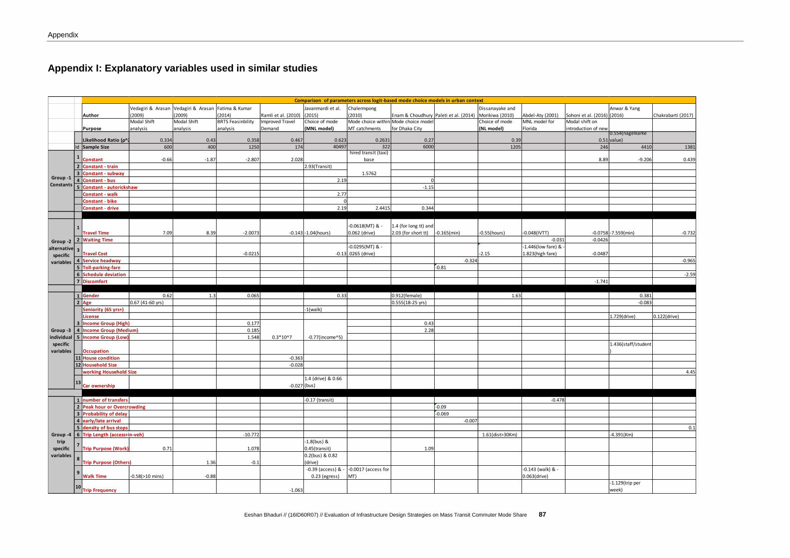
Appendix
Eeshan Bhaduri // (16ID60R07) // Evaluation of Infrastructure Design Strategies on Mass Transit Commuter Mode Share 87
Appendix I: Explanatory variables used in similar studies
Author
Vedagiri & Arasan
(2009)
Vedagiri & Arasan
(2009)
Fatima & Kumar
(2014) Ramli et al. (2010)
Javanmardi et al.
(2015)
Wibowo &
Chalermpong
(2010) Enam & Choudhury Paleti et al. (2014)
Dissanayake and
Morikiwa (2010) Abdel-Aty (2001) Sohoni et al. (2016)
Anwar & Yang
(2016) Chakrabarti (2017)
Purpose
Modal Shift
analysis
Modal Shift
analysis
BRTS Feasinbility
analysis
Improved Travel
Demand
Choice of mode
(MNL model)
Mode choice within
MT catchments
Mode choice model
for Dhaka City
Choice of mode
(NL model)
MNL model for
Florida
Modal shift on
introduction of new
Likelihood Ratio (ρ^2) 0.334 0.43 0.358 0.467 0.623 0.2631 0.27 0.39 0.51
0.554(nagelkarke
value)
Id Sample Size 600 400 1250 174 40497 322 6000 1205 246 4410 1381
1Constant -0.66 -1.87 -2.807 2.028
hired transit (taxi)
base 8.89 -9.206 0.439
2 Constant - train 2.93(Transit)
3 Constant - subway
4 Constant - bus 2.19 0
5 Constant - autorickshaw -1.15
Constant - walk 2.77
Constant - bike 0
Constant - drive 2.19 2.4415 0.344
1Travel Time 7.09 8.39 -2.0073 -0.143 -1.04(hours)
-0.0618(MT) & -
0.062 (drive)
1.4 (for long tt) and
2.03 (for short tt) -0.165(min) -0.55(hours) -0.048(IVTT) -0.0758 -7.559(min) -0.732
2 Waiting Time -0.031 -0.0426
3Travel Cost -0.0215 -0.13
-0.0295(MT) & -
.0265 (drive) -2.15
-1.446(low fare) & -
1.823(high fare) -0.0487
4 Service headway -0.324 -0.965
5 Toll-parking-fare -0.81
6 Schedule deviation -2.59
7 Discomfort -1.741
1 Gender 0.62 1.3 0.065 0.33 0.912(female) 1.63 0.381
2 Age 0.67 (41-60 yrs) 0.555(18-25 yrs) -0.083
Seniority (65 yrs+) -1(walk)
License 1.729(drive) 0.122(drive)
3 Income Group (High) 0.177 0.43
4 Income Group (Medium) 0.185 2.28
5 Income Group (Low) 1.548
Occupation
1.436(staff/student
)
11 House condition -0.363
12 Household Size -0.028
working Household Size 4.45
13Car ownership -0.027
1.4 (drive) & 0.66
(bus)
1 number of transfers -0.17 (transit) -0.478
2 Peak hour or Overcrowding -0.09
3 Probability of delay -0.069
4 early/late arrival -0.007
5 density of bus stops 0.1
6 Trip Length (access+in-veh) -10.772 1.61(dist>30Km) -4.391(Km)
7Trip Purpose (Work) 0.71 1.078
-1.8(bus) &
0.45(transit) 1.09
8Trip Purpose (Others) 1.36 -0.1
0.2(bus) & 0.82
(drive)
9Walk Time -0.58(>10 mins) -0.88
-0.39 (access) & -
0.23 (egress)
-0.0017 (access for
MT)
-0.143 (walk) & -
0.063(drive)
10Trip Frequency -1.063
-1.129(trip per
week)
Comparison of parameters across logit-based mode choice models in urban context
0.3*10^7 -0.77(income^5)
Group -1
Constants
Group -3
individual
specific
variables
Group -4
trip
specific
variables
1.5762
Group -2
alternative
specific
variables

Appendix
Eeshan Bhaduri // (16ID60R07) // Evaluation of Infrastructure Design Strategies on Mass Transit Commuter Mode Share 88
Appendix II: R Results development
Atte
mpt
Id
Variables Coeff. R^2 t -
value
%
insig.
Remarks
1 tot_time_hr -6.58 0.33 -9.28 0 single coefficient for time for
all 4 modes
2 tot_time_hr 0.45 28 positive coeff. For train
3 tot_time_hr+age 0.33 72 negative coeff.for age For all
3 modes but none significant
4 tot_time_hr+age+gender 0.36 80 negative coeff.for age For all
3 modes but none significant +
negative coeff.for subway and
positive for bus & train but
none significant
4A tot_time_hr+I(bus*age)+I(bu
s*gender)+I(subway*age)+I(
subway*gender)
0.34 80 bus:gender becomes too
insignificant (strange !!!)
4B tot_time_hr+I(bus*age)+I(bu
s*gender)+I(subway*age)+I(
subway*gender)+I(bus*peak
_hr)+I(subway*peak_hr)
0.35 bus:gender becomes slighlty
more significant and peak
hour for both bus & subway is
near significance threshold
4C tot_time_hr+I(bus*age)+I(b
us*gender)+I(subway*age)
+I(subway*gender)+I(bus*
peak_hr)+I(subway*peak_h
r)+I(subway*trip_pur)
0.35
5
subway:trip_pur has a
negative coefficient
5 tot_time_hr+whh_size 0.33 42 negative coeff.for subway &
bus (more negative for
subway) and positive for train
but none significant

Appendix
Eeshan Bhaduri // (16ID60R07) // Evaluation of Infrastructure Design Strategies on Mass Transit Commuter Mode Share 89
Appendix III: Dataset arranged in wide format (sample)
mode age age_1 age_2 age_3 age_4 genderveh_availa
bilitypeak_hr trip_pur trip_HBW trip_HBE trip_HBO alt TT_hr freq_hr chid
1.ar FALSE 3 0 1 0 0 1 0 1 4 1 0 0 ar 0.425 10 1
1.bus TRUE 3 0 1 0 0 1 0 1 4 1 0 0 bus 0.34 7.5 1
1.subway FALSE 3 0 1 0 0 1 0 1 4 1 0 0 subway 0.2444444 10 1
1.train FALSE 3 0 1 0 0 1 0 1 4 1 0 0 train 0.38 3 1
2.ar TRUE 4 0 0 1 0 1 0 1 2 1 0 0 ar 0.2787879 10 2
2.bus FALSE 4 0 0 1 0 1 0 1 2 1 0 0 bus 0.76875 7.5 2
2.subway FALSE 4 0 0 1 0 1 0 1 2 1 0 0 subway 0.2694444 10 2
2.train FALSE 4 0 0 1 0 1 0 1 2 1 0 0 train 0.4825 3 2
3.ar TRUE 4 0 0 1 0 1 0 1 2 1 0 0 ar 0.3060606 10 3
3.bus FALSE 4 0 0 1 0 1 0 1 2 1 0 0 bus 0.80625 7.5 3
3.subway FALSE 4 0 0 1 0 1 0 1 2 1 0 0 subway 0.2861111 10 3
3.train FALSE 4 0 0 1 0 1 0 1 2 1 0 0 train 0.4975 3 3
4.ar FALSE 3 0 1 0 0 1 0 1 2 1 0 0 ar 1.03125 10 4
4.bus TRUE 3 0 1 0 0 1 0 1 2 1 0 0 bus 0.7515152 7.5 4
4.subway FALSE 3 0 1 0 0 1 0 1 2 1 0 0 subway 0.5416667 10 4
4.train FALSE 3 0 1 0 0 1 0 1 2 1 0 0 train 0.7275 3 4
5.ar FALSE 3 0 1 0 0 1 0 1 2 1 0 0 ar 0.69375 10 5
5.bus TRUE 3 0 1 0 0 1 0 1 2 1 0 0 bus 0.5666667 7.5 5
5.subway FALSE 3 0 1 0 0 1 0 1 2 1 0 0 subway 0.3638889 10 5
5.train FALSE 3 0 1 0 0 1 0 1 2 1 0 0 train 0.4875 3 5
6.ar FALSE 3 0 1 0 0 1 0 1 2 1 0 0 ar 0.2625 10 6
6.bus TRUE 3 0 1 0 0 1 0 1 2 1 0 0 bus 0.17 7.5 6
6.subway FALSE 3 0 1 0 0 1 0 1 2 1 0 0 subway 0.1722222 10 6
6.train FALSE 3 0 1 0 0 1 0 1 2 1 0 0 train 0.315 3 6
7.ar TRUE 4 0 0 1 0 1 0 1 4 1 0 0 ar 0.719697 10 7
7.bus FALSE 4 0 0 1 0 1 0 1 4 1 0 0 bus 1.03125 7.5 7
7.subway FALSE 4 0 0 1 0 1 0 1 4 1 0 0 subway 0.3861111 10 7
7.train FALSE 4 0 0 1 0 1 0 1 4 1 0 0 train 0.5875 3 7
8.ar TRUE 4 0 0 1 0 0 1 1 2 1 0 0 ar 0.7090909 10 8
8.bus FALSE 4 0 0 1 0 0 1 1 2 1 0 0 bus 1.13125 7.5 8
8.subway FALSE 4 0 0 1 0 0 1 1 2 1 0 0 subway 0.4305556 10 8
8.train FALSE 4 0 0 1 0 0 1 1 2 1 0 0 train 0.6275 3 8
9.ar FALSE 3 0 1 0 0 0 1 1 2 1 0 0 ar 0.75625 10 9
9.bus TRUE 3 0 1 0 0 0 1 1 2 1 0 0 bus 0.5627273 7.5 9
9.subway FALSE 3 0 1 0 0 0 1 1 2 1 0 0 subway 0.4194444 10 9
9.train FALSE 3 0 1 0 0 0 1 1 2 1 0 0 train 0.6175 3 9
10.ar TRUE 4 0 0 1 0 1 0 1 2 1 0 0 ar 0.4166667 10 10
10.bus FALSE 4 0 0 1 0 1 0 1 2 1 0 0 bus 0.84375 7.5 10
10.subway FALSE 4 0 0 1 0 1 0 1 2 1 0 0 subway 0.3027778 10 10
10.train FALSE 4 0 0 1 0 1 0 1 2 1 0 0 train 0.5125 3 10
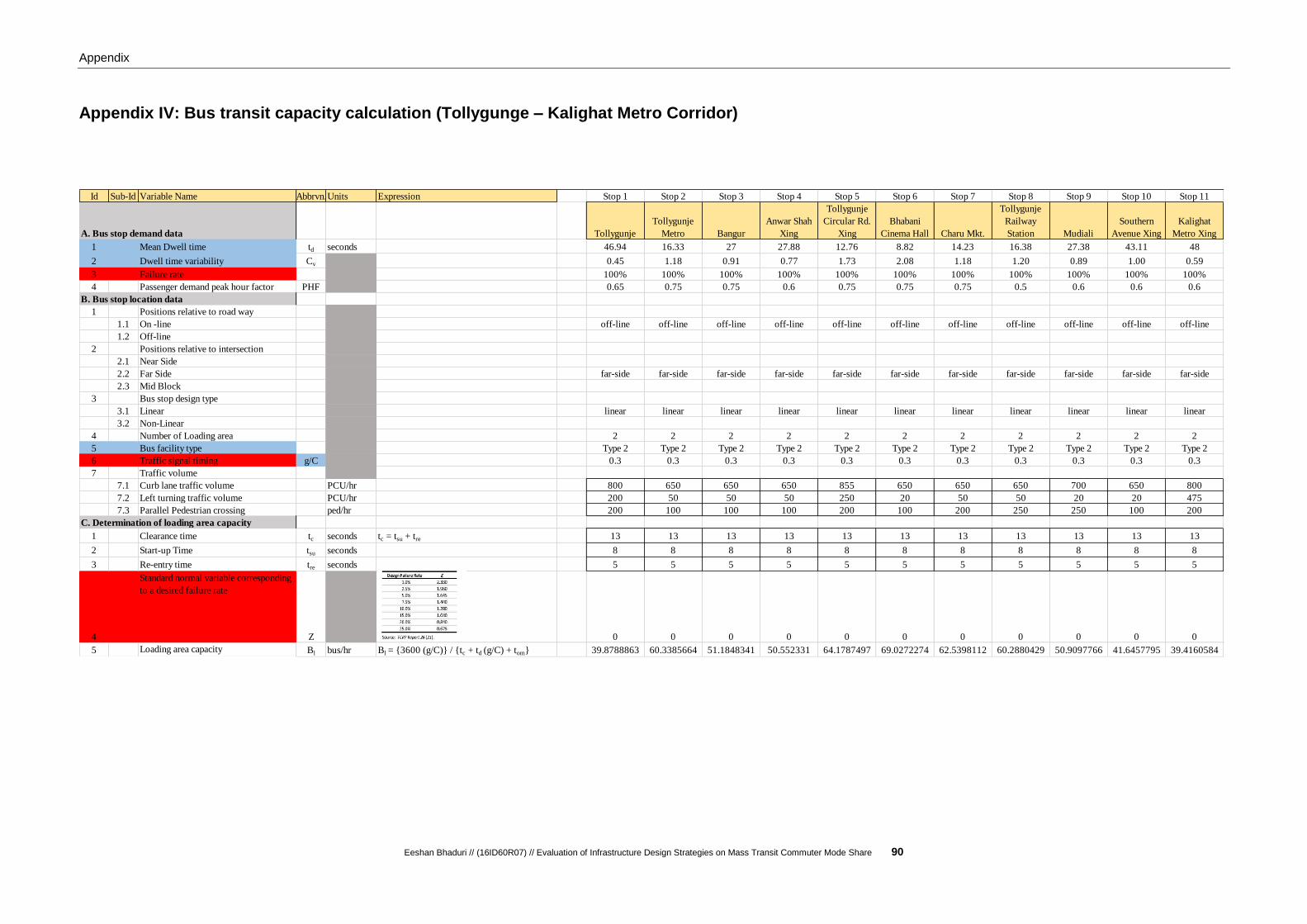
Appendix
Eeshan Bhaduri // (16ID60R07) // Evaluation of Infrastructure Design Strategies on Mass Transit Commuter Mode Share 90
Appendix IV: Bus transit capacity calculation (Tollygunge – Kalighat Metro Corridor)
Id Sub-Id Variable Name Abbrvn.Units Expression Stop 1 Stop 2 Stop 3 Stop 4 Stop 5 Stop 6 Stop 7 Stop 8 Stop 9 Stop 10 Stop 11
Tollygunje
Tollygunje
Metro Bangur
Anwar Shah
Tollygunje
Circular Rd.
Bhabani
Cinema Hall Charu Mkt.
Tollygunje
Railway
Station Mudiali
Southern
Avenue Xing
Kalighat
Metro Xing
1 Mean Dwell time td seconds 46.94 16.33 27 27.88 12.76 8.82 14.23 16.38 27.38 43.11 48
2 Dwell time variability Cv 0.45 1.18 0.91 0.77 1.73 2.08 1.18 1.20 0.89 1.00 0.59
3 Failure rate 100% 100% 100% 100% 100% 100% 100% 100% 100% 100% 100%
4 Passenger demand peak hour factor PHF 0.65 0.75 0.75 0.6 0.75 0.75 0.75 0.5 0.6 0.6 0.6
1 Positions relative to road way
1.1 On -line off-line off-line off-line off-line off-line off-line off-line off-line off-line off-line off-line
1.2 Off-line
2 Positions relative to intersection
2.1 Near Side
2.2 Far Side far-side far-side far-side far-side far-side far-side far-side far-side far-side far-side far-side
2.3 Mid Block
3 Bus stop design type
3.1 Linear linear linear linear linear linear linear linear linear linear linear linear
3.2 Non-Linear
4 Number of Loading area 2 2 2 2 2 2 2 2 2 2 2
5 Bus facility type Type 2 Type 2 Type 2 Type 2 Type 2 Type 2 Type 2 Type 2 Type 2 Type 2 Type 2
6 Traffic signal timing g/C 0.3 0.3 0.3 0.3 0.3 0.3 0.3 0.3 0.3 0.3 0.3
7 Traffic volume
7.1 Curb lane traffic volume PCU/hr 800 650 650 650 855 650 650 650 700 650 800
7.2 Left turning traffic volume PCU/hr 200 50 50 50 250 20 50 50 20 20 475
7.3 Parallel Pedestrian crossing ped/hr 200 100 100 100 200 100 200 250 250 100 200
1 Clearance time tc seconds tc = tsu + tre 13 13 13 13 13 13 13 13 13 13 13
2 Start-up Time tsu seconds 8 8 8 8 8 8 8 8 8 8 8
3 Re-entry time tre seconds 5 5 5 5 5 5 5 5 5 5 5
4
Standard normal variable corresponding
to a desired failure rate
Z 0 0 0 0 0 0 0 0 0 0 0
5 Loading area capacity Bl bus/hr Bl = {3600 (g/C)} / {tc + td (g/C) + tom} 39.8788863 60.3385664 51.1848341 50.552331 64.1787497 69.0272274 62.5398112 60.2880429 50.9097766 41.6457795 39.4160584
A. Bus stop demand data
B. Bus stop location data
C. Determination of loading area capacity
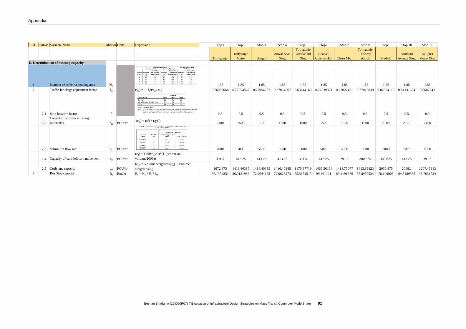
Appendix
Eeshan Bhaduri // (16ID60R07) // Evaluation of Infrastructure Design Strategies on Mass Transit Commuter Mode Share 91
Id Sub-Id Variable Name Abbrvn.Units Expression Stop 1 Stop 2 Stop 3 Stop 4 Stop 5 Stop 6 Stop 7 Stop 8 Stop 9 Stop 10 Stop 11
Tollygunje
Tollygunje
Metro Bangur
Anwar Shah
Tollygunje
Circular Rd.
Bhabani
Cinema Hall Charu Mkt.
Tollygunje
Railway
Station Mudiali
Southern
Avenue Xing
Kalighat
Metro Xing
1 Number of effective loading area Nel 1.85 1.85 1.85 1.85 1.85 1.85 1.85 1.85 1.85 1.85 1.85
2 Traffic blockage adjustment factor ftb (ftb) = 1- fl*(vcl / ccl) 0.76089068 0.77054567 0.77054567 0.77054567 0.63644163 0.77839321 0.77027431 0.77013839 0.82934113 0.84131634 0.6687242
2.1 Stop location factor fl 0.5 0.5 0.5 0.5 0.5 0.5 0.5 0.5 0.5 0.5 0.5
2.2
Capacity of curb lane through
movement cth PCU/hr (cth) = (sf) * (g/C)
2100 1500 1500 1500 1500 1500 1500 1500 2100 2100 2400
2.3 Saturation flow rate sf PCU/hr 7000 5000 5000 5000 5000 5000 5000 5000 7000 7000 8000
2.4 Capacity of curb left turn movement clt PCU/hr
(clt) = 1450*(g/C)*(1-(pedestrian
volume/2000)) 391.5 413.25 413.25 413.25 391.5 413.25 391.5 380.625 380.625 413.25 391.5
2.5 Curb lane capacity ccl PCU/hr
(ccl) = Volume weighted (cth) + Volume
weighted (clt) 1672.875 1416.40385 1416.40385 1416.40385 1175.87719 1466.56154 1414.73077 1413.89423 2050.875 2048.1 1207.45313
3 Bus Stop capacity Bs Bus/hr Bs = Nel * Bl * ftb 56.1354251 86.0131986 72.9644665 72.0628273 75.5651515 99.401101 89.1196986 85.8957524 78.109908 64.8189585 48.7631734
D. Determination of bus stop capacity

Appendix
Eeshan Bhaduri // (16ID60R07) // Evaluation of Infrastructure Design Strategies on Mass Transit Commuter Mode Share 92
Appendix V: Bus transit speed calculation (Tollygunge – Kalighat
Metro Corridor)
Id Id Variable Name Abbrvn. Units Expression Full Stretch
1 average stop spacing Ns Stops/Km 3.6
2 average dwell time td seconds 26.25727273
3 scheduled number of buses at critical stop Bus/hr 94
4 traffic signal timing and phasing Signals/Km 3
5 traffic interference
48.76317341
1 Time spent at running speed trs seconds (trs) = Lrs / (cf * vrun) 37.74844604
1.1 Bus running speed on facility vrun Km/hr 50
1.2 Conversion factor cf 0.278
1.3 Distance travelled at running speed per Km Lrs metres (Lrs) = Lmk – Ns Lad 524.7034
1.4 Length of a mile or Km Lmk 1000
2Distance travelled at less than running speed
Lad metres(Lad) = 0.5*a*(tacc)
2+0.5*d*(tdec)
2+ Lsta 132.0268333
2.1 Acceleration time tacc seconds (tacc) = (cf * vrun) / a 11.58333333
2.2 Deceleration time tdec seconds (tdec) = (cf * vrun) / d 9.266666667
2.3 time required to travel through station tsta seconds (tsta) = Lsta / (1/ cf*vst - 1/ cf*vrun) 0
2.4 Average Bus acceleration a m/s^2 1.2
2.5 Average Bus deceleration d m/s^2 1.5
2.6 Bus speed through station vst Km/hr 0 if not busway operation 0
2.7 Length of Station Lsta metres 0 if not busway operation 0
3 unimpeded bus running time rate tu minutes/Km tu = { trs + Ns ( td + tacc + tdec + tsta )} / 60 3.455577131
4 additional running time losses tl minutes/Km 0
5 base bus running time rate tr minutes/Km tr = tu + tl 3.455577131
Skip-stop factor fsp 1 if no skip stop 1
bus v/c
Scheduled no. of Bus in per hour / Max capacity of
street 1.927684222
bus-bus interference factor fbb 0.60
Section running time rate ts minutes/Km (ts) = tr / fbb * fsp 5.781289502
Average Section speed Ss Km/hr (Ss) = 60/ ts 10.37830747
A. Bus stop demand data
B. Determination of base bus running time rate
C. Adjust for skip-stop operation
D. Adjust for bus congestion
E. Determination of average section speed
A1. Determination of section maximum capacity
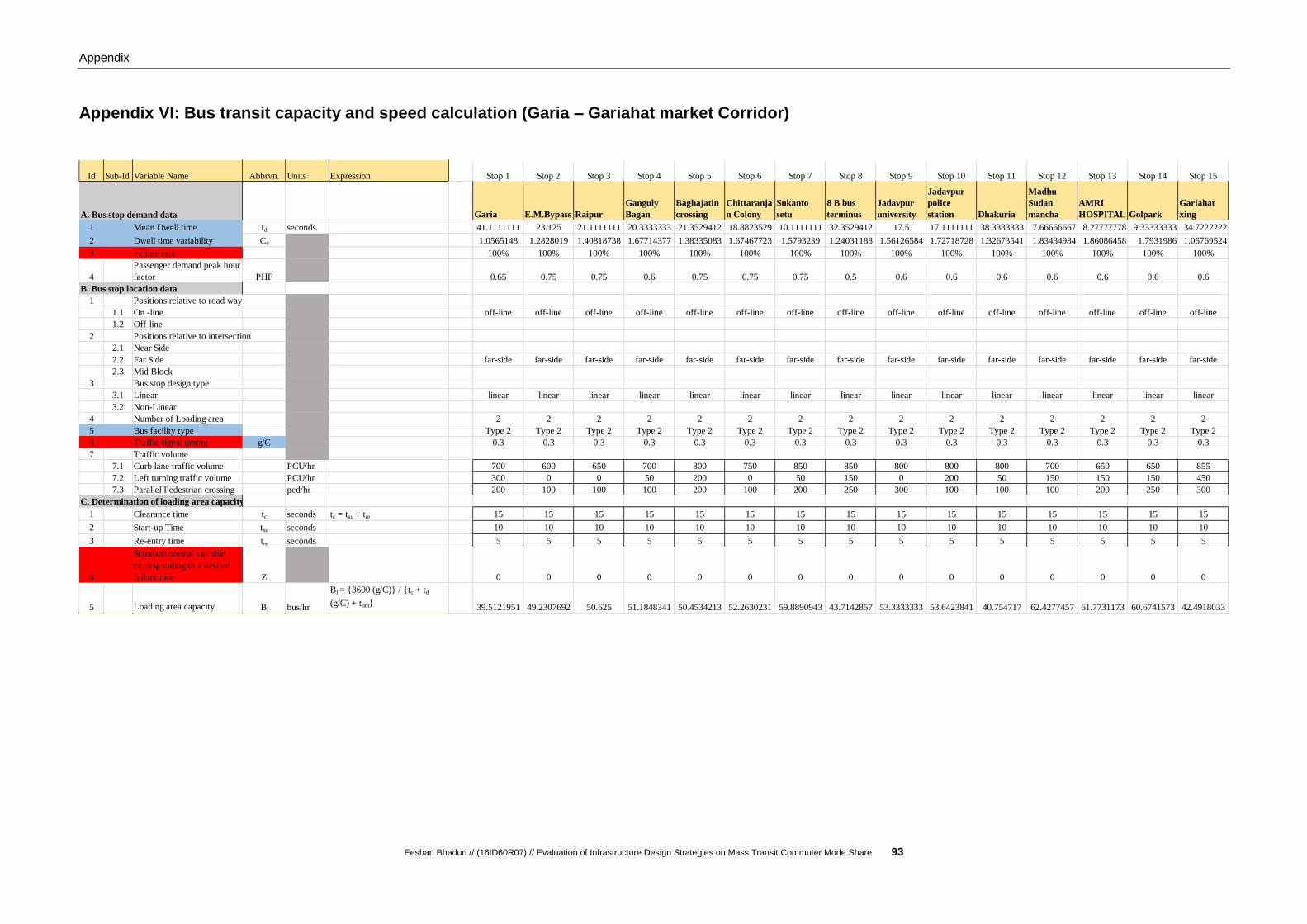
Appendix
Eeshan Bhaduri // (16ID60R07) // Evaluation of Infrastructure Design Strategies on Mass Transit Commuter Mode Share 93
Appendix VI: Bus transit capacity and speed calculation (Garia – Gariahat market Corridor)
Id Sub-Id Variable Name Abbrvn. Units Expression Stop 1 Stop 2 Stop 3 Stop 4 Stop 5 Stop 6 Stop 7 Stop 8 Stop 9 Stop 10 Stop 11 Stop 12 Stop 13 Stop 14 Stop 15
Garia E.M.Bypass Raipur
Ganguly
Bagan
Baghajatin
crossing
Chittaranja
n Colony
Sukanto
setu
8 B bus
terminus
Jadavpur
university
Jadavpur
police
station Dhakuria
Madhu
Sudan
mancha
AMRI
HOSPITAL Golpark
Gariahat
1 Mean Dwell time td seconds 41.1111111 23.125 21.1111111 20.3333333 21.3529412 18.8823529 10.1111111 32.3529412 17.5 17.1111111 38.3333333 7.66666667 8.27777778 9.33333333 34.7222222
2 Dwell time variability Cv 1.0565148 1.2828019 1.40818738 1.67714377 1.38335083 1.67467723 1.5793239 1.24031188 1.56126584 1.72718728 1.32673541 1.83434984 1.86086458 1.7931986 1.06769524
3 Failure rate 100% 100% 100% 100% 100% 100% 100% 100% 100% 100% 100% 100% 100% 100% 100%
4
Passenger demand peak hour
factor PHF 0.65 0.75 0.75 0.6 0.75 0.75 0.75 0.5 0.6 0.6 0.6 0.6 0.6 0.6 0.6
1 Positions relative to road way
1.1 On -line off-line off-line off-line off-line off-line off-line off-line off-line off-line off-line off-line off-line off-line off-line off-line
1.2 Off-line
2 Positions relative to intersection
2.1 Near Side
2.2 Far Side far-side far-side far-side far-side far-side far-side far-side far-side far-side far-side far-side far-side far-side far-side far-side
2.3 Mid Block
3 Bus stop design type
3.1 Linear linear linear linear linear linear linear linear linear linear linear linear linear linear linear linear
3.2 Non-Linear
4 Number of Loading area 2 2 2 2 2 2 2 2 2 2 2 2 2 2 2
5 Bus facility type Type 2 Type 2 Type 2 Type 2 Type 2 Type 2 Type 2 Type 2 Type 2 Type 2 Type 2 Type 2 Type 2 Type 2 Type 2
6 Traffic signal timing g/C 0.3 0.3 0.3 0.3 0.3 0.3 0.3 0.3 0.3 0.3 0.3 0.3 0.3 0.3 0.3
7 Traffic volume
7.1 Curb lane traffic volume PCU/hr 700 600 650 700 800 750 850 850 800 800 800 700 650 650 855
7.2 Left turning traffic volume PCU/hr 300 0 0 50 200 0 50 150 0 200 50 150 150 150 450
7.3 Parallel Pedestrian crossing ped/hr 200 100 100 100 200 100 200 250 300 100 100 100 200 250 300
1 Clearance time tc seconds tc = tsu + tre 15 15 15 15 15 15 15 15 15 15 15 15 15 15 15
2 Start-up Time tsu seconds 10 10 10 10 10 10 10 10 10 10 10 10 10 10 10
3 Re-entry time tre seconds 5 5 5 5 5 5 5 5 5 5 5 5 5 5 5
4
Standard normal variable
corresponding to a desired
failure rate Z 0 0 0 0 0 0 0 0 0 0 0 0 0 0 0
5 Loading area capacity Bl bus/hr
Bl = {3600 (g/C)} / {tc + td
(g/C) + tom}39.5121951 49.2307692 50.625 51.1848341 50.4534213 52.2630231 59.8890943 43.7142857 53.3333333 53.6423841 40.754717 62.4277457 61.7731173 60.6741573 42.4918033
A. Bus stop demand data
B. Bus stop location data
C. Determination of loading area capacity

Appendix
Eeshan Bhaduri // (16ID60R07) // Evaluation of Infrastructure Design Strategies on Mass Transit Commuter Mode Share 94
Id Sub-Id Variable Name Abbrvn. Units Expression Stop 1 Stop 2 Stop 3 Stop 4 Stop 5 Stop 6 Stop 7 Stop 8 Stop 9 Stop 10 Stop 11 Stop 12 Stop 13 Stop 14 Stop 15
Garia E.M.Bypass Raipur
Ganguly
Bagan
Baghajatin
crossing
Chittaranja
n Colony
Sukanto
setu
8 B bus
terminus
Jadavpur
university
Jadavpur
police
station Dhakuria
Madhu
Sudan
mancha
AMRI
HOSPITAL Golpark
Gariahat
1
Number of effective loading
area Nel 1.85 1.85 1.85 1.85 1.85 1.85 1.85 1.85 1.85 1.85 1.85 1.85 1.85 1.85 1.85
2
Traffic blockage adjustment
factor ftb (ftb) = 1- fl*(vcl / ccl) 0.70744522 0.8 0.78333333 0.75393268 0.67290197 0.75 0.70379025 0.6736952 0.80952381 0.76166536 0.72068563 0.72378416 0.73878636 0.80918508 0.59178289
2.1 Stop location factor fl far-side and type 2 0.5 0.5 0.5 0.5 0.5 0.5 0.5 0.5 0.5 0.5 0.5 0.5 0.5 0.5 0.5
2.2
Capacity of curb lane through
movement cth veh/hr (cth) = (sf) * (g/C)
1800 1500 1500 1500 1500 1500 1500 1500 2100 2100 1500 1500 1500 2100 1800
2.3 Saturation flow rate sf veh/hr 6000 5000 5000 5000 5000 5000 5000 5000 7000 7000 5000 5000 5000 7000 6000
2.4
Capacity of curb left turn
movement clt veh/hr
(clt) = 1450*(g/C)*(1-
(pedestrian volume/2000)) 391.5 413.25 413.25 413.25 391.5 413.25 391.5 380.625 369.75 413.25 413.25 413.25 391.5 380.625 369.75
2.5 Curb lane capacity ccl veh/hr
(ccl) = Volume weighted (cth) +
Volume weighted (clt) 1196.35714 1500 1500 1422.375 1222.875 1500 1434.79412 1302.46324 2100 1678.3125 1432.07813 1267.125 1244.19231 1703.22115 1047.23684
3 Bus Stop capacity Bs Bus/hr Bs = Nel * Bl * ftb 51.7125202 72.8615385 73.3640625 71.3913507 62.8078824 72.5149445 77.9763177 54.4826936 79.8730159 75.5864601 54.3369769 83.5907946 84.4287026 90.8287528 46.5199558
D. Determination of bus stop capacity

Appendix
Eeshan Bhaduri // (16ID60R07) // Evaluation of Infrastructure Design Strategies on Mass Transit Commuter Mode Share 95
Appendix VII: Bus transit capacity and speed calculation (Garia –
Gariahat market Corridor)
Id Id Variable Name Abbrvn. Units Expression Corridor
Existing
1 average stop spacing Ns Stops/Km 2.08
2 average dwell time td seconds 21.4216231
3
scheduled number of buses at
critical stop Bus/hr 94
4 traffic signal timing and phasing Signals/Km 3
5 traffic interference
46.5199558
1 Time spent at running speed trs seconds (trs) = Lrs / (cf * vrun) 52.1859127
1.1 Bus running speed on facility vrun Km/hr 50
1.2 Conversion factor cf 0.278
1.3
Distance travelled at running
speed per Km Lrs metres (Lrs) = Lmk – Ns Lad 725.384187
1.4 Length of a mile or Km Lmk 1000
2
Distance travelled at less than
running speed Lad metres
(Lad) =
0.5*a*(tacc)2+0.5*d*(tdec)
2+ Lsta
132.026833
2.1 Acceleration time tacc seconds (tacc) = (cf * vrun) / a 11.5833333
2.2 Deceleration time tdec seconds (tdec) = (cf * vrun) / d 9.26666667
2.3
time required to travel through
station tsta seconds (tsta) = Lsta / (1/ cf*vst - 1/ cf*vrun) 0
2.4 Average Bus acceleration a m/s^2 1.2
2.5 Average Bus deceleration d m/s^2 1.5
2.6 Bus speed through station vst Km/hr 0 if not busway operation 0
2.7 Length of Station Lsta metres 0 if not busway operation 0
3 Unimpeded bus running time rate tu minutes/Km
tu = { trs + Ns ( td + tacc + tdec +
tsta )} / 60 2.33518148
4 Additional running time losses tl minutes/Km 0
5 Base bus running time rate tr minutes/Km tr = tu + tl 2.33518148
Skip-stop factor fsp 1 if no skip stop 1
bus v/c
Scheduled no. of Bus in per
hour / Max capacity of street 2.02063821
bus-bus interference factor fbb 0.57
Section running time rate ts minutes/Km (ts) = tr / fbb * fsp 4.06158329
Average Section speed Ss Km/hr (Ss) = 60/ ts 14.7725642
A. Bus stop demand data
A1. Determination of section maximum
B. Determination of base bus running time
C. Adjust for skip-stop operation
D. Adjust for bus congestion
E. Determination of average section speed

Appendix
Eeshan Bhaduri // (16ID60R07) // Evaluation of Infrastructure Design Strategies on Mass Transit Commuter Mode Share 96
Appendix VIII: Detailed sub-scenarios of Scenario 1 – Improvement in existing network (Capacity improvement)
Id Time Impact
Cost Impact Speed Constraints Capacity Constraints Change in variables Methods
Stretch applicability
1.01
•Average Dwell time •Dwell time variability
•Average Dwell time = 45 sec / 30 sec •Dwell time variability = 0.6
•Reduce dwell time based on TCRP calculation •Reduce variability based on TCRP calculation (average value)
All
1.02
•Dwell time improvisation •Bus priority signalling
•Average Dwell time = 45 sec / 30 sec •Dwell time variability = 0.6 •g/C Ratio = 0.4
•Reduce dwell time based on TCRP calculation •Reduce variability based on TCRP calculation (average value) •Increase g/C ratio
All
1.03
•Dwell time improvisation •Introduction of near side stop •Bus priority signalling
•Average Dwell time = 45 sec / 30 sec •Dwell time variability = 0.6 •g/C Ratio = 0.4 •stop location factor = 0.90 (type 2 lane)
•Reduce dwell time based on TCRP calculation •Reduce variability based on TCRP calculation (average value) •Change type of bus stop factor •Increase g/C ratio
All
1.04
•Dwell time improvisation •Bus priority signalling •Use queue jumps and curb extension
•Average Dwell time = 45 sec / 30 sec •Dwell time variability = 0.7 •g/C Ratio = 0.45 •bus priority design = NO re entry delay
•Reduction in Re-entry time (reduction in dwell time)
All
1.05
•Dwell time improvisation •Remove auto-rickshaw from arterial streets
•Average Dwell time = 45 sec / 30 sec •curb lane volume = no auto-rickshaw
•Reduce dwell time based on TCRP calculation •Reduce variability based on TCRP calculation (average value) •Decrease the Traffic volume
Selected
1.06
•Dwell time improvisation •Remove on-street Parking
•Average Dwell time = 45 sec / 30 sec •saturation flow = increased
•Reduce dwell time based on TCRP calculation •Reduce variability based on TCRP calculation (average value) •Increase saturation volume of the street
Selected
1.07
•Dwell time improvisation •Bus priority signalling •Remove auto-rickshaw from arterial streets •Use queue jumps and curb extension •Remove on-street Parking
•Average Dwell time = 45 sec / 30 sec •Dwell time variability = 0.6 •g/C Ratio = 0.45 •bus priority design = NO re entry delay •saturation flow = increased •curb lane volume = no auto-rickshaw
Selected
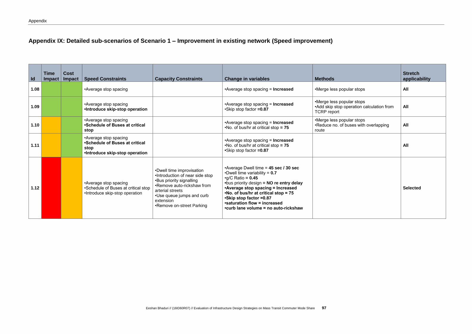
Appendix
Eeshan Bhaduri // (16ID60R07) // Evaluation of Infrastructure Design Strategies on Mass Transit Commuter Mode Share 97
Appendix IX: Detailed sub-scenarios of Scenario 1 – Improvement in existing network (Speed improvement)
Id Time Impact
Cost Impact Speed Constraints Capacity Constraints Change in variables Methods
Stretch applicability
1.08 •Average stop spacing •Average stop spacing = Increased •Merge less popular stops All
1.09 •Average stop spacing •Introduce skip-stop operation
•Average stop spacing = Increased •Skip stop factor =0.87
•Merge less popular stops •Add skip stop operation calculation from TCRP report
All
1.10 •Average stop spacing •Schedule of Buses at critical stop
•Average stop spacing = Increased •No. of bus/hr at critical stop = 75
•Merge less popular stops •Reduce no. of buses with overlapping route
All
1.11
•Average stop spacing •Schedule of Buses at critical stop •Introduce skip-stop operation
•Average stop spacing = Increased •No. of bus/hr at critical stop = 75 •Skip stop factor =0.87
All
1.12 •Average stop spacing •Schedule of Buses at critical stop •Introduce skip-stop operation
•Dwell time improvisation •Introduction of near side stop •Bus priority signalling •Remove auto-rickshaw from arterial streets •Use queue jumps and curb extension •Remove on-street Parking
•Average Dwell time = 45 sec / 30 sec •Dwell time variability = 0.7 •g/C Ratio = 0.45 •bus priority design = NO re entry delay •Average stop spacing = Increased •No. of bus/hr at critical stop = 75 •Skip stop factor =0.87 •saturation flow = increased •curb lane volume = no auto-rickshaw
Selected
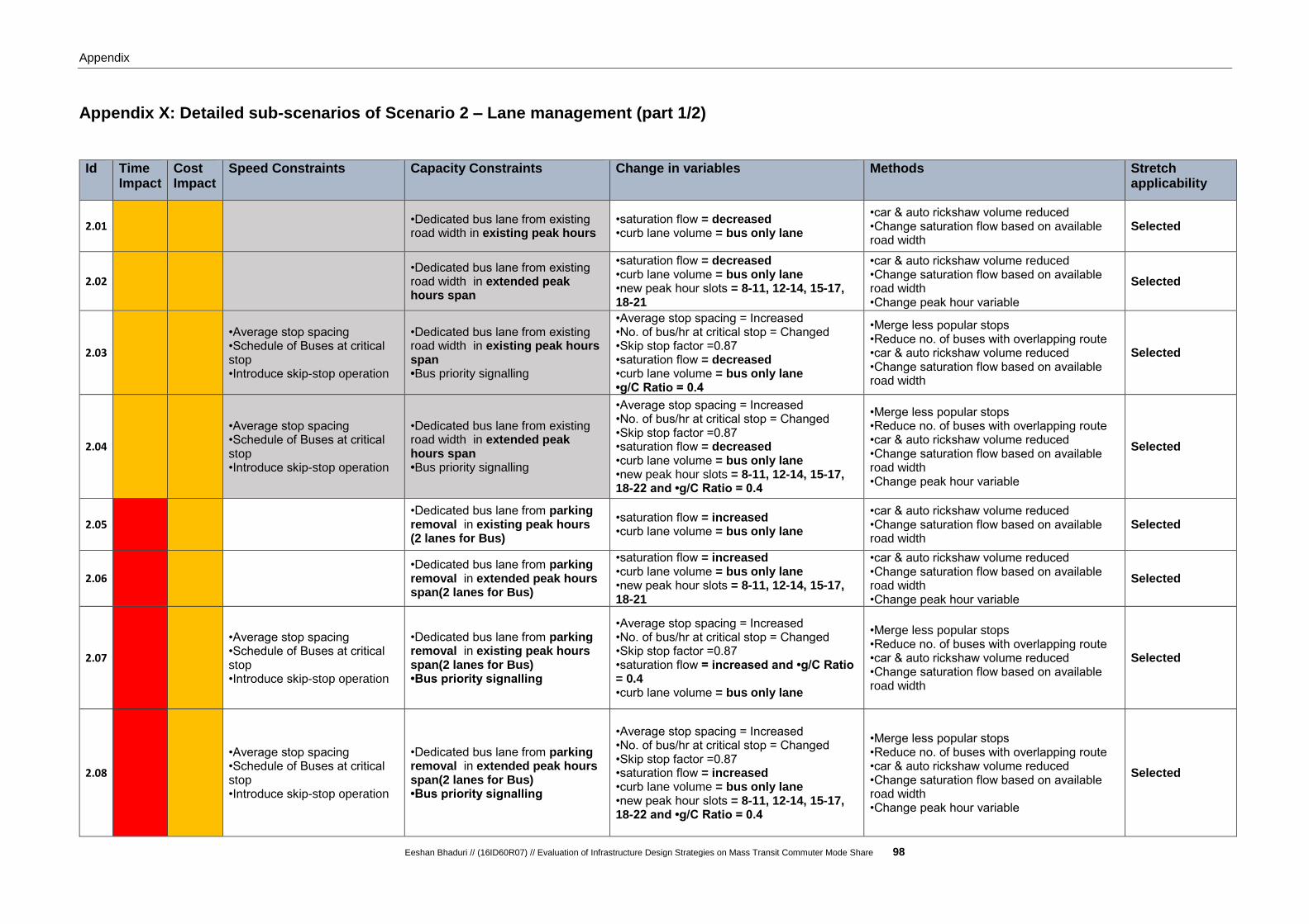
Appendix
Eeshan Bhaduri // (16ID60R07) // Evaluation of Infrastructure Design Strategies on Mass Transit Commuter Mode Share 98
Appendix X: Detailed sub-scenarios of Scenario 2 – Lane management (part 1/2)
Id Time Impact
Cost Impact
Speed Constraints Capacity Constraints Change in variables Methods Stretch applicability
2.01 •Dedicated bus lane from existing road width in existing peak hours
•saturation flow = decreased •curb lane volume = bus only lane
•car & auto rickshaw volume reduced •Change saturation flow based on available road width
Selected
2.02 •Dedicated bus lane from existing road width in extended peak hours span
•saturation flow = decreased •curb lane volume = bus only lane •new peak hour slots = 8-11, 12-14, 15-17, 18-21
•car & auto rickshaw volume reduced •Change saturation flow based on available road width •Change peak hour variable
Selected
2.03
•Average stop spacing •Schedule of Buses at critical stop •Introduce skip-stop operation
•Dedicated bus lane from existing road width in existing peak hours span •Bus priority signalling
•Average stop spacing = Increased •No. of bus/hr at critical stop = Changed •Skip stop factor =0.87 •saturation flow = decreased •curb lane volume = bus only lane •g/C Ratio = 0.4
•Merge less popular stops •Reduce no. of buses with overlapping route •car & auto rickshaw volume reduced •Change saturation flow based on available road width
Selected
2.04
•Average stop spacing •Schedule of Buses at critical stop •Introduce skip-stop operation
•Dedicated bus lane from existing road width in extended peak hours span •Bus priority signalling
•Average stop spacing = Increased •No. of bus/hr at critical stop = Changed •Skip stop factor =0.87 •saturation flow = decreased •curb lane volume = bus only lane •new peak hour slots = 8-11, 12-14, 15-17, 18-22 and •g/C Ratio = 0.4
•Merge less popular stops •Reduce no. of buses with overlapping route •car & auto rickshaw volume reduced •Change saturation flow based on available road width •Change peak hour variable
Selected
2.05 •Dedicated bus lane from parking removal in existing peak hours (2 lanes for Bus)
•saturation flow = increased •curb lane volume = bus only lane
•car & auto rickshaw volume reduced •Change saturation flow based on available road width
Selected
2.06 •Dedicated bus lane from parking removal in extended peak hours span(2 lanes for Bus)
•saturation flow = increased •curb lane volume = bus only lane •new peak hour slots = 8-11, 12-14, 15-17, 18-21
•car & auto rickshaw volume reduced •Change saturation flow based on available road width •Change peak hour variable
Selected
2.07
•Average stop spacing •Schedule of Buses at critical stop •Introduce skip-stop operation
•Dedicated bus lane from parking removal in existing peak hours span(2 lanes for Bus) •Bus priority signalling
•Average stop spacing = Increased •No. of bus/hr at critical stop = Changed •Skip stop factor =0.87 •saturation flow = increased and •g/C Ratio = 0.4 •curb lane volume = bus only lane
•Merge less popular stops •Reduce no. of buses with overlapping route •car & auto rickshaw volume reduced •Change saturation flow based on available road width
Selected
2.08
•Average stop spacing •Schedule of Buses at critical stop •Introduce skip-stop operation
•Dedicated bus lane from parking removal in extended peak hours span(2 lanes for Bus) •Bus priority signalling
•Average stop spacing = Increased •No. of bus/hr at critical stop = Changed •Skip stop factor =0.87 •saturation flow = increased •curb lane volume = bus only lane •new peak hour slots = 8-11, 12-14, 15-17, 18-22 and •g/C Ratio = 0.4
•Merge less popular stops •Reduce no. of buses with overlapping route •car & auto rickshaw volume reduced •Change saturation flow based on available road width •Change peak hour variable
Selected

Appendix
Eeshan Bhaduri // (16ID60R07) // Evaluation of Infrastructure Design Strategies on Mass Transit Commuter Mode Share 99
Appendix X: Detailed sub-scenarios of Scenario 2 – Lane management (part 2/2)
Id Time Impact
Cost Impact
Speed Constraints Capacity Constraints Change in variables Methods Stretch applicability
2.09 •Introducing contraflow car lane in existing peak hours (NO car allowed on peak direction)
•saturation flow = same •curb lane volume = decreased by 50%
•car & auto rickshaw volume reduced •Change saturation flow based on available road width
Selected
2.1 •Introducing contraflow car lane in extended peak hours span (NO car allowed on peak direction)
•saturation flow = same •curb lane volume = decreased by 50% •new peak hour slots = 8-11, 12-14, 15-17, 18-21
•car & auto rickshaw volume reduced •Change saturation flow based on available road width •Change peak hour variable
Selected
2.11
•Average stop spacing •Schedule of Buses at critical stop •Introduce skip-stop operation
•Introducing contraflow car lane in existing peak hours span (NO car allowed on peak direction) •Bus priority signalling
•Average stop spacing = Increased •No. of bus/hr at critical stop = Changed •Skip stop factor =0.87 •saturation flow = same •curb lane volume = decreased by 50% •g/C Ratio = 0.4
•Merge less popular stops •Reduce no. of buses with overlapping route •car & auto rickshaw volume reduced •Change saturation flow based on available road width
Selected
2.12
•Average stop spacing •Schedule of Buses at critical stop •Introduce skip-stop operation
•Introducing contraflow car lane in extended peak hours span (NO car allowed on peak direction) •Bus priority signalling
•Average stop spacing = Increased •No. of bus/hr at critical stop = Changed •Skip stop factor =0.87 •saturation flow = same •curb lane volume = decreased by 50% •new peak hour slots = 8-11, 12-14, 15-17, 18-22 and •g/C Ratio = 0.4
•Merge less popular stops •Reduce no. of buses with overlapping route •car & auto rickshaw volume reduced •Change saturation flow based on available road width •Change peak hour variable
Selected
2.13
•Introducing contraflow car lane in existing peak hours (NO car allowed on peak direction) •Removal of Auto-Rickshaw
•saturation flow = same •curb lane volume = decreased by 60%
•car & auto rickshaw volume reduced •Change saturation flow based on available road width
Selected
2.14
•Introducing contraflow car lane in extended peak hours span (NO car allowed on peak direction) •Removal of Auto-Rickshaw
•saturation flow = same •curb lane volume = decreased by 60% •new peak hour slots = 8-11, 12-14, 15-17, 18-21
•car & auto rickshaw volume reduced •Change saturation flow based on available road width •Change peak hour variable
Selected
2.15
•Average stop spacing •Schedule of Buses at critical stop •Introduce skip-stop operation
•Introducing contraflow car lane in existing peak hours (NO car allowed on peak direction) •Removal of Auto-Rickshaw from arterial street •Bus priority signalling
•Average stop spacing = Increased •No. of bus/hr at critical stop = Changed •Skip stop factor =0.87 •saturation flow = same •curb lane volume = decreased by 60% •g/C Ratio = 0.4
•Merge less popular stops •Reduce no. of buses with overlapping route •car & auto rickshaw volume reduced •Change saturation flow based on available road width
Selected
2.16
•Average stop spacing •Schedule of Buses at critical stop •Introduce skip-stop operation
•Introducing contraflow car lane in extended peak hours span (NO car allowed on peak direction) •Removal of Auto-Rickshaw from arterial street •Bus priority signalling
•Average stop spacing = Increased •No. of bus/hr at critical stop = Changed. •Skip stop factor =0.87 •saturation flow = same •curb lane volume = decreased by 60% •new peak hour slots = 8-11, 12-14, 15-17, 18-22 and •g/C Ratio = 0.4
•Merge less popular stops •Reduce no. of buses with overlapping route •car & auto rickshaw volume reduced •Change saturation flow based on available road width •Change peak hour variable
Selected

Appendix
Eeshan Bhaduri // (16ID60R07) // Evaluation of Infrastructure Design Strategies on Mass Transit Commuter Mode Share 100
Appendix XI: Detailed sub-scenarios of Scenario 3 – Introduction of new transit service BRTS
Id Time Impact
Cost Impact
Speed Constraints Capacity Constraints Change in variables Methods Stretch applicability
3.01
•24 hrs Grade separated bus lane from parking removal (1 lane for Bus+1 lane for BRTS) •Bus priority signalling
•Saturation flow = increased for BRTS / decreased for Bus •curb lane volume = increased for Bus / decreased for BRTS •g/C Ratio = 0.4
•Calculate changed vehicular speeds for BRTS buses based on traffic volume change •Calculate changed vehicular speeds for other Buses based on traffic volume change •Calculate changed vehicular speeds for auto-rickshaw mode •Calculate changed waiting time
Selected
3.02
•Average stop spacing •Schedule of Buse`s at critical stop •Introduce skip-stop operation
•24 hrs Grade separated bus lane from parking removal (1 lane for Bus+1 lane for BRTS) •Bus priority signalling
•saturation flow = increased for BRTS / decreased for Bus •curb lane volume = increased for Bus / decreased for BRTS •Average stop spacing = Increased •No. of bus/hr at critical stop = 75 •Skip stop factor =0.87 •g/C Ratio = 0.4
•Calculate changed vehicular speeds for BRTS buses based on traffic volume change •Calculate changed vehicular speeds for other Buses based on traffic volume change •Calculate changed vehicular speeds for auto-rickshaw mode •Calculate changed waiting time
Selected