evaluation of interior low-e storm windows in the … evaluation of interior low-e storm windows in...
TRANSCRIPT

PNNL-24827
Prepared for the U.S. Department of Energy under Contract DE-AC05-76RL01830
Evaluation of Interior Low-E Storm Windows in the PNNL Lab Homes October 2015
JM Petersen MB Merzouk GP Sullivan V Srivastava KA Cort JM Weber


PNNL-24827
Evaluation of Interior Low-E Storm Windows in the PNNL Lab Homes JM Petersen MB Merzouk GP Sullivan V Srivastava KA Cort JM Weber October 2015 Prepared for the U.S. Department of Energy under Contract DE-AC05-76RL01830 and the Northwest Energy Efficiency Alliance under Contract 67620 Pacific Northwest National Laboratory Richland, Washington 99352

iii
Summary
To examine the energy and air-leakage performance of interior low-emissivity (low-e) storm windows in a residential retrofit application, a field evaluation was undertaken in a matched pair of all-electric, factory-built “lab homes” located on the Pacific Northwest National Laboratory (PNNL) campus in Richland, Washington. The 1500-square-foot homes were identical in construction and baseline performance, which allowed any difference in energy and thermal performance between the baseline home (Lab Home A) and the experimental home (Lab Home B) to be attributed to the interior low-E storm windows installed in the experimental home.
To assess performance in a residential retrofit application, interior low-e storm windows were installed in the experimental home behind 74% of the window area. The primary windows in both Lab Homes are identical double-pane, clear-glass, and aluminum-frame. The building shell air leakage, energy use, and interior temperatures of each home were compared during the 2014–2015 winter heating and 2015 summer cooling seasons. The results of the experiment confirm that low-e storm windows reduce heating and cooling loads in the home when installed behind primary windows. The measured energy savings averaged 8.1% for the heating season and 4.2% for the cooling season for identical occupancy conditions. To extrapolate the annual energy savings from the seasonal measured data, EnergyPlus simulations were used to reflect observed load profiles and onsite weather data. The modeled annual HVAC energy savings from the installation of the low-e interior storm over approximately 74% of the window area was 7.8% or 1,006 kWh/yr.
Interior low-e storm windows affect whole-house and HVAC energy use by:
1. Reducing conductive heat transfer due to the better insulating capabilities
2. Reducing convective heat transfer due to the extra glass layer and airspace, as well as improved air-tightness around the primary window openings
3. Reducing radiative energy losses due to the low-e coating
4. Reducing solar gains due to a slightly lower solar heat gain coefficient (SHGC)
The test results suggest that the energy savings were primarily realized due to the decreased U-factor through the window, with no significant changes observed in infiltration. The low-e storm windows did not significantly decrease the air leakage of the home due to the fact that the primary windows were already well-sealed. For homes with “leakier” older windows or envelope, the storm windows would likely generate more savings than observed in this study.
The Lab Homes allow for the performance of low-e storm window energy savings to be accurately measured in a controlled setting. Additional studies are needed to fully document the performance of low-e storm windows across a variety of building types and climate zones and determine the cost-effectiveness of low-e storm windows in a variety of retrofit scenarios; however, the data clearly demonstrate that low-e storm windows can be an effective energy-saving measure that should be considered for retrofits in residential buildings.


v
Acknowledgments
The authors would like to thank Tom Culp of Birch Point Consulting who assisted in the preparation of this document by providing input and graphics.
The authors would also like to thank Quanta Technologies for providing the interior low-e storm windows for the Lab Home experiments.


vii
Acronyms and Abbreviations
ACH50 air changes per hour at 50 Pascals of depressurization with respect to the outside BTP Building Technologies Program Btu British thermal unit CDD cooling degree days cfm cubic feet per minute cfm50 cubic feet per minute at 50 Pascals of depressurization with respect to outside CU condensing unit d day(s) DOE U.S. Department of Energy ET Emerging Technologies °F Fahrenheit ft foot (feet) HDD heating degree days hr hour(s) HVAC heating, ventilation, and air-conditioning kW kilowatt(s) kWh kilowatt hour LBNL Lawrence Berkeley National Laboratory low-e low-emissivity MRT meant radiant temperature NAHB National Association of Home Builders NEAT National Energy Audit Tool NFRC National Fenestration Rating Council Pa Pascal(s) RECS Renewable Energy Consumption Survey RESFEN RESidential FENestration SEER seasonal energy-efficiency ratio SHGC solar heat gain coefficient WAP Weatherization Assistance Program Wh watt-hour(s) W/m2 watts per square meter yr year(s)


ix
Contents
Summary ...................................................................................................................................................... iii Acknowledgments ......................................................................................................................................... v Acronyms and Abbreviations ..................................................................................................................... vii 1.0 Introduction .......................................................................................................................................... 1 2.0 Background ........................................................................................................................................... 2
2.1 Low-E Storm Windows Technology ............................................................................................ 2 2.2 Low-E Storm Windows Development and Previous Research .................................................... 3 2.3 Summarized Case Studies ............................................................................................................ 4
3.0 Experimental Design ............................................................................................................................ 7 3.1 Lab Homes ................................................................................................................................... 7 3.2 Windows Retrofit ......................................................................................................................... 8
3.2.1 Interior Low-E Storm Window Performance Ratings ....................................................... 9 3.3 Experimental Timeline ............................................................................................................... 10 3.4 Metering Approach .................................................................................................................... 11
4.0 Results and Discussion ....................................................................................................................... 14 4.1 Baseline Performance ................................................................................................................. 14 4.2 Building Shell Air Leakage ........................................................................................................ 16 4.3 Low-E Storm Window Energy Performance ............................................................................. 17
4.3.1 Winter Heating Season Results ....................................................................................... 18 4.3.2 Summer Cooling Season Results .................................................................................... 20 4.3.3 Temperature Profile ......................................................................................................... 20 4.3.4 Dependence on Outdoor Air Temperature and Solar Insolation ..................................... 22
4.4 Average Annual Savings ............................................................................................................ 28 4.5 Interior Temperature Distributions ............................................................................................. 28
5.0 Interior and Exterior Storm Window Comparison ............................................................................. 31 6.0 Conclusions ........................................................................................................................................ 32 7.0 References .......................................................................................................................................... 33 Appendix A – Installation Process for Low-E Interior Storm Windows ...................................................... 1
x
Figures
Figure 2.1. Representation of Light and Heat Transfer with Low-e Coating ............................................... 3 Figure 3.1. Floor Plan of the Lab Homes as Constructed ............................................................................. 7 Figure 3.2. Interior Storm Window Weather Stripping and Installation ....................................................... 9 Figure 3.3. Interior Storm Window Temperature Measurement Points ...................................................... 13 Figure 4.1. HVAC Energy Use of Experimental Home (Red) and Baseline Home (Blue) during
Heating Season Baselining of the Homes ........................................................................................... 15 Figure 4.2. Cumulative HVAC Energy Use of the Experimental Home (Red) and the Baseline
Home (Blue) throughout one day of the Baseline Period ................................................................... 16 Figure 4.3. Baseline Home (Blue) and Experimental Home (Red) HVAC Energy use compared to
Average Outdoor Air Temperature during the Winter Heating Season .............................................. 18 Figure 4.4. Baseline Home Master Bedroom Exterior (left), Experimental Home Master Bedroom
Exterior (right) .................................................................................................................................... 19 Figure 4.5. Baseline Home Master Bedroom Interior (left), Experimental Home Master Bedroom Interior
(right)1 ................................................................................................................................................. 19 Figure 4.6. Percent HVAC Energy Savings compared to Peak outdoor air temperature over the
Summer Cooling Season ..................................................................................................................... 20 Figure 4.8. Temperature comparison of exterior window glass between Baseline Home A (Blue)
and Experimental Home B (Green) During the Heating Season ........................................................ 21 Figure 4.9. Temperature Surface Gradient between Baseline Home (Lab A) and Experimental Home (Lab
B) During the Heating Season ............................................................................................................ 22 Figure 4.10. HVAC Energy Use (Wh/d; left axis) and HVAC Energy Savings (%; right axis) Versus
Average Outdoor Air Temperature (°F) ............................................................................................. 23 Figure 4.11. HVAC Energy Use and Indoor Temperature for the Experimental Home (red and purple
lines) and the Baseline Home (blue and orange lines) on a Warm, Sunny Day (8/10/2015) ............. 24 Figure 4.12. Cumulative HVAC Energy Use of the Experimental Home (Red) and Baseline Home
(Blue) on a typical day during the Cooling Season ............................................................................ 25 Figure 4.13. HVAC Energy Use and Indoor Temperature for the Experimental Home (red and purple
lines) and the Baseline Home (blue and orange lines) on a Sunny Day (2/11/2015) ......................... 26 Figure 4.14. Cumulative Energy Use of the Experimental Home (Red) Versus the Baseline Home
(Blue) during the Heating Season ....................................................................................................... 27 Figure 4.15. Percent HVAC Energy Savings Compared to Measured Solar Insolation ............................. 27 Figure 4.16. Interior Temperature Distribution for Lab Home A (left) and Lab Home B (right) on
2/15/215, a Sunny Day in the Heating Season .................................................................................... 29 Figure 4.17. Interior Temperature Distribution for Lab Home A (left) and Lab Home B (right) on
8/11/2015, a Hot Sunny Day in the Cooling Season ........................................................................... 30

xi
Tables
Table 2.1. Summarized Case Studies Focused on Low-E Storm Windows ................................................. 5 Table 3.1. Primary Window and Combined System Characteristics ............................................................ 9 Table 3.2. Experimental Timeline............................................................................................................... 10 Table 3.3. Electrical Points Monitored ....................................................................................................... 11 Table 3.4. Temperature and Environmental Points Monitored ................................................................... 12 Table 4.1. Blower Door Test Results Pre and Post Storm Windows Installation ....................................... 17

1
1.0 Introduction
Residential buildings in the United States currently require approximately 8 quadrillion Btu of energy per year for heating and cooling, which accounts for about 40% of the primary energy consumed by homes.1 Windows are a major source of heating losses and gains in residential buildings because of their heat transfer and infiltration properties, especially relative to other building shell components. For example, it has been estimated that windows account for approximately 25% of the energy use in a typical residential building (Huang et al. 1999). Despite this fact, approximately three quarters of US homes are equipped with low-performing single-pane or double-pane clear-glass windows. Even though approximately 30 million windows are replaced each year with higher-performing, insulated windows (AAMA 2012),2 these lower-performing windows continue to remain prevalent. While the window industry has made many advances in energy efficiency over the last decade, the installation of low-emissivity (low-e) double-pane windows appears to have been limited primarily to new housing and major remodeling projects, in part because of the relatively high cost of these windows.
A number of in-home field studies, as well one controlled whole home experiment (Knox and Widder 2014), have demonstrated the ability of low-e storm windows to reduce energy use when installed over primary windows of all types. Following on a 2014 study in the Pacific Northwest National Laboratory’s (PNNL) matched pair of Lab Homes3, which focused on the application of exterior low-e storm windows, this study evaluates the energy savings potential of installing interior low-e storm windows4 behind typical double-pane clear-glass aluminum-frame windows. This report describes whole home experimental research conducted in support of Building America’s Window Attachments program and the Northwest Energy Efficiency Alliance (NEEA). The U.S. Department of Energy’s (DOE) Building America Program serves as a catalyst to accelerate the residential building energy-efficiency market transformation and support increasing levels of cost-effective whole-house energy savings. NEEA is an alliance of more than 140 Northwest utilities and energy efficiency organizations working on behalf of more than 13 million energy consumers.5 Its mission is to accelerate both electric and gas energy efficiency, leveraging regional partnerships to advance the adoption of energy-efficient products.
In the Pacific Northwest, a recently conducted study found that although an estimated 87% of residential single-family customers in the region (Oregon, Washington, Montana, and Idaho) have double-pane windows, many of these double-pane windows are low-performing clear glass windows, similar to the windows installed in the Pacific Northwest National Laboratory’s (PNNL) Lab Homes. Based on the survey information, an estimated 44% of existing homes in the region have low-performing (single-pane or double-pane clear) windows. In addition, only a small percentage (approximately 15%) of these homes had some form of storm windows installed over the primary windows. Window performance for multi-family homes in the Northwest follows a similar pattern to the single-family homes (Baylon et al. 2013). In addition, the majority of windows in commercial buildings across the region are also lower-performing windows; approximately 73% are double-pane windows made up of clear glass, and 74% are metal
1“Residential sector key indicators and consumption.” Annual Energy Outlook (DOE). Available online: http://www.eia.gov/forecasts/aeo/pdf/tbla4.pdf 2 Single-pane estimates are from Renewable Energy Consumption Survey (RECS) 2009 (47.2 million homes or ~40%). Although the 2009 RECS did not include estimates of double-pane clear windows, the 2005 RECS estimated 50.6 million homes with double-pane clear windows (DOE-EIA 2005). The current estimate is based on estimates of prime window replacements (AAMA 2012) during the time frame and window trends between the 2005 and 2009 RECS. This corresponds with an estimate of 46 million homes, or nearly 40% of the residential homes. 3 See http://labhomes.pnnl.gov for more information on Lab Homes. 4 Interior low-e storm windows are often also referred to as low-e insulating panels. 5 See http://neea.org/about-neea for more information (accessed September 2015).
2
framed windows (Navigant 2014). Although there are over 50 utility programs in the Northwest providing incentives for window replacement1, the 2013 Home Energy Rating Program data shows that window replacements are still only conducted under 10% of all retrofit projects2, likely due to the relatively high initial cost of this measure. Adding low-e interior and exterior storm windows offers utilities and homeowners a lower-cost alternative to the replacement of primary windows, while still gaining most of the energy benefit.
The purpose of this project is to evaluate the energy savings potential of interior low-e storm windows by installing this technology is just one of the two identical Lab Homes. The energy use of each home’s heating, ventilation, and air conditioning (HVAC) system is compared during both the heating and cooling seasons. Both homes deploy identical simulated occupancy schedules so that the performance and effects of the low-e storm windows is isolated from all other variables. The results from the research, as presented in this report, help validate savings and performance of installing low-e storm windows behind double-pane clear primary windows.
2.0 Background
Storm windows have been a technology option for improving the performance of existing windows for decades. Recent advances in storm window technology have improved storm window designs to incorporate low-e coatings and a variety of operable configurations, increasing the energy performance and utility of storm windows. Today’s storm windows can be permanently installed in homes and case studies have demonstrated how they can save energy in residential homes in multiple climate zones including the Northwest.
2.1 Low-E Storm Windows Technology
Traditional storm windows consisted of a single piece of clear glass (or plastic) in a wood or aluminum frame and were installed on the outside of an existing window. Modern storm windows can be operable or fixed in place and come in a variety of configurations and trim colors. They typically have insert screens to allow for natural ventilation, tighter seals for less air leakage, and are intended to be permanently mounted. Typical low-e storm windows look just like other modern storm windows, but include a low-e pyrolytic coating that lowers the emissivity of glass, effectively reducing the heat transmission through the storm window. The pyrolytic coat is a hard tin-oxide–based ceramic coating deposited onto the glass during the float glass process3 that is durable and can withstand the elements, unlike soft-coat or sputtered low-e coatings that are more typical of primary windows and must be protected in a sealed double pane unit.
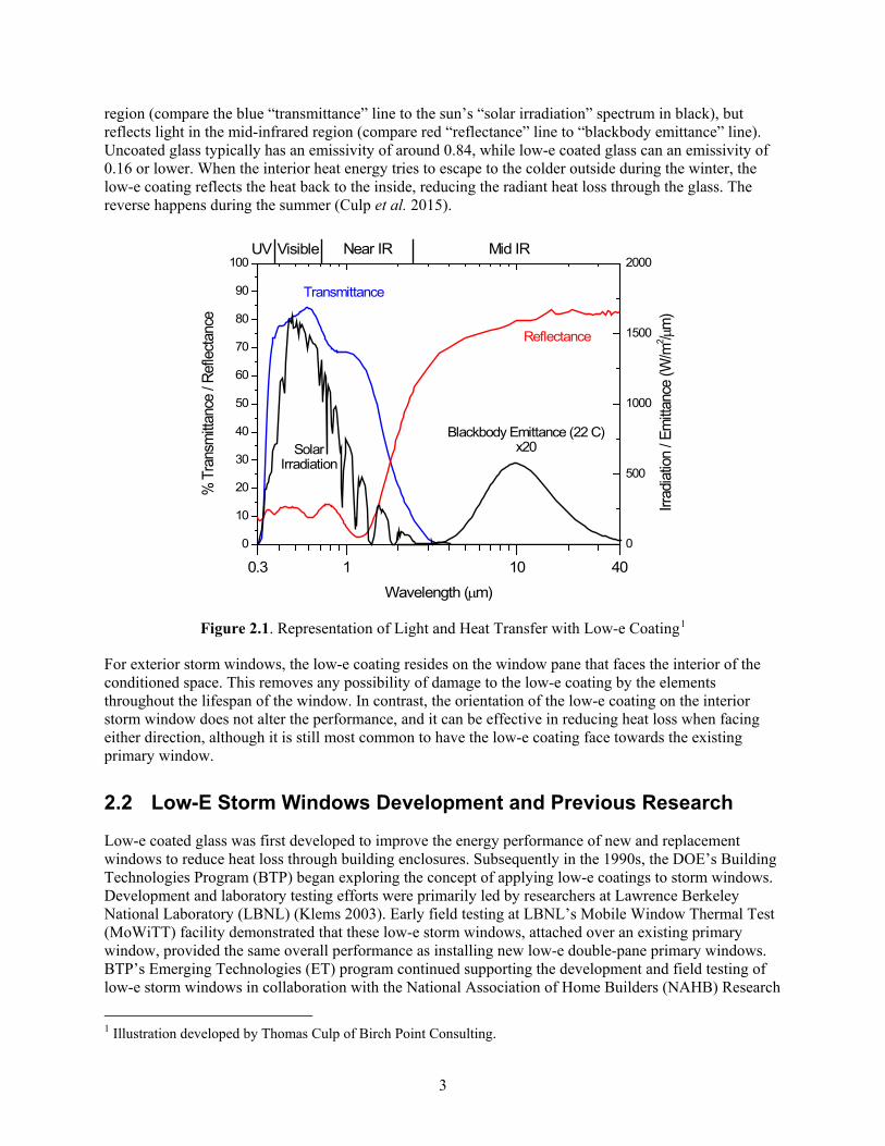
All materials, including windows, radiate heat in the form of long-wave infrared energy depending on the emissivity and temperature of their surfaces. Radiant energy is one of the important ways heat transfer occurs with windows. Low-e coatings are microscopic coatings that reflect infrared heat. The coating consists of very thin, electrically conductive material, which is transparent in visible region and reflective in infrared spectrum. Figure 2.1 illustrates this effect, where the coating transmits light in the visible 1 Based on DSIRE database search available online at: http://www.dsireusa.org/ 2 Energy Trust of Oregon (2014). Based on data from 2,000 audited homes (primarily in Oregon). See http://rtf.nwcouncil.org//meetings/2014/04/Default.asp, presentation: Measure Interactions for Residential Single Family SEEM-affected UES Measures - Back to "Option 3"? 3 The float glass process is how window glass is made. It involved floating molten silica, combined with soda lime and other elements, on a bed of molten tin and then cooling the glass in a controlled environment.
3
region (compare the blue “transmittance” line to the sun’s “solar irradiation” spectrum in black), but reflects light in the mid-infrared region (compare red “reflectance” line to “blackbody emittance” line). Uncoated glass typically has an emissivity of around 0.84, while low-e coated glass can an emissivity of 0.16 or lower. When the interior heat energy tries to escape to the colder outside during the winter, the low-e coating reflects the heat back to the inside, reducing the radiant heat loss through the glass. The reverse happens during the summer (Culp et al. 2015).
Figure 2.1. Representation of Light and Heat Transfer with Low-e Coating1
For exterior storm windows, the low-e coating resides on the window pane that faces the interior of the conditioned space. This removes any possibility of damage to the low-e coating by the elements throughout the lifespan of the window. In contrast, the orientation of the low-e coating on the interior storm window does not alter the performance, and it can be effective in reducing heat loss when facing either direction, although it is still most common to have the low-e coating face towards the existing primary window.
2.2 Low-E Storm Windows Development and Previous Research
Low-e coated glass was first developed to improve the energy performance of new and replacement windows to reduce heat loss through building enclosures. Subsequently in the 1990s, the DOE’s Building Technologies Program (BTP) began exploring the concept of applying low-e coatings to storm windows. Development and laboratory testing efforts were primarily led by researchers at Lawrence Berkeley National Laboratory (LBNL) (Klems 2003). Early field testing at LBNL’s Mobile Window Thermal Test (MoWiTT) facility demonstrated that these low-e storm windows, attached over an existing primary window, provided the same overall performance as installing new low-e double-pane primary windows. BTP’s Emerging Technologies (ET) program continued supporting the development and field testing of low-e storm windows in collaboration with the National Association of Home Builders (NAHB) Research
1 Illustration developed by Thomas Culp of Birch Point Consulting.
0.3 1 10 400
10
20
30
40
50
60
70
80
90
100Mid IRNear IRVisibleUV
Transmittance
SolarIrradiation
Reflectance
Blackbody Emittance (22 C)x20
% T
rans
mitta
nce
/ Ref
lecta
nce
Wavelength (µm)
0
500
1000
1500
2000
Irra
diatio
n / E
mitta
nce
(W/m
2 /µm)
4
Center and Utilivate Technologies (Drumheller et al. 2007). The ET team also supported demonstrations of the technology with case studies and initiated deployment efforts by including low-e storm windows as part of its windows volume purchase market transformation program (Parker et al. 2013). ET continued to fund field case studies and educational programs (Quanta Technologies 2013), and initiated a pilot program to integrate low-e storm windows as a qualified weatherization measure in Pennsylvania as part of DOE’s Weatherization Assistance Program (WAP) (Krigger and Van der Meer 2011).
In 2014, PNNL led the evaluation of exterior storm windows in the Lab Homes during the heating and cooling seasons (Knox and Widder 2014). Measured HVAC savings due to the exterior storm windows averaged 10.5% for the heating season and 8.0% for the cooling season for identical occupancy conditions. Extrapolating these energy savings numbers based on typical average heating degree days and cooling degree days per year yields an estimated annual HVAC energy savings of 10.1%. (Knox and Widder 2014).
2.3 Summarized Case Studies
A series of laboratory tests have proven that low-e storm windows save energy at the component level. The performance improvements have been validated with field tests and case studies supported by BTP’s ET team. The approaches and results of these field tests and case studies are described and summarized in previous reports (Cort 2013) and a high-level summary of these activities is provided in Table 2.1.
In addition to case studies, a number of climate-based modeling efforts have been performed to examine the potential energy savings and the cost effectiveness of installing low-e storm windows over existing windows in residential homes across a broad range of U.S. climate zones. Calculations of energy savings and the cost effectiveness of low-e storm windows have been conducted with two software platforms: the National Energy Audit Tool (NEAT), used by weatherization programs, and RESFEN (RESidential FENestration) software, used to compare the annual energy performance of different window options in single-family homes (Culp and Cort 2014). In the Pacific Northwest, the Regional Technical Forum (RTF1) conducted a modeling study low-e storm windows using its Simplified Energy Enthalpy Model (SEEM)2 in 2015. The results of this study demonstrated that low-e storm windows met the criteria to be considered a “proven” and cost-effective energy saving measure in the Bonneville Power Administration region (includes Oregon, Washington, Idaho, and part of Montana).3
1 The RTF is an advisory committee for the Northwest Power & Conservation Council established to develop standards to verify and evaluate energy savings from technologies, approaches, systems, and measures for the Bonneville Power Administration. 2 The SEEM program is designed to model small scale residential building energy use and consists of hourly thermal simulation and humidity simulation that interacts with duct specifications, equipment, and water parameters to calculate the annual heating and cooling energy requirements of the home. 3Meeting minutes and RTF staff presentations are available online: http://rtf.nwcouncil.org/meetings/2015/07/minutes20150721.pdf (accessed September 2015)

5
Table 2.1. Summarized Case Studies Focused on Low-E Storm Windows
Study Sponsor Baseline Description Findings Chicago Case Study (2007)
DOE, HUD, NAHB
Research Center, LBNL
6 low-income homes; single-pane wood-framed windows
• 21% reduction in overall home heating load • 7% reduction in overall home air infiltration • Simple payback of 4 to 5 years
Infrared Camera Imaging
DOE, LBNL, Building Green
Single-pane wood-framed windows
Images showed that interior low-e storm windows performed equivalently or better than new double-pane replacement windows with low-e glass and argon fill
Atlanta Case Study (2-year study)
DOE, Quanta,(a) Larson,(b)
NAHB RC, AGC Flat Glass, and
NSG-Pilkington
10 occupied homes; single-pane wood-framed windows
High variability, but approximately: • ~15% heating energy reduction • ~2 to 30% cooling reduction (highly variable) • 17% reduction in overall home air infiltration
Philadelphia Multifamily Case Study
DOE, Quanta, Larson, NAHB RC, AGC Flat Glass, NSG-Pilkington
2 large multifamily buildings; single-pane, metal framed windows
Replacing old clear glass storm windows with new low-E storm windows provided: • 18%–22% reduction in heating energy use • 9% reduction in cooling energy use • 10% reduction in overall apartment air leakage
Field Air-Leakage Testing (Bronx, NY, 2013)
Steven Winter Associates,
Quanta
Multifamily dwellings in Bronx
Interior low-E panels reduced the effective leakage area by: • 77% for windows without air-conditioning units • 95% for windows with air-conditioning units
Pennsylvania Weatherization technical support (2010)
DOE, Birch Point
Consulting
37 model homes with range of window types
Modeled results for 7 climate zones: • 12%–33% overall HVAC savings
PNNL Lab Homes study exterior low-e storm windows (controlled whole experiment, 2014)
DOE 2 controlled test homes with double-pane clear windows
Annual average of 10% HVAC savings (limited effect from infiltration due to tight baseline windows) • 10.5% heating savings • 8% cooling savings
(a) Quanta Technologies, Inc., Malvern, Pennsylvania. (b) Larson Manufacturing Company, Brookings, South Dakota. Sources and documentation for case study results include Drumheller et al. (2007), Quanta Technologies (2013), Zalis et al. (2010), and Knox and Widder (2014). AGC = Asahi Glass Company; HUD = U.S. Department of Housing and Urban Development; LBNL = Lawrence Berkeley National Laboratory; NAHB = National Association of Home Builders.
Although field data and case studies provide valuable insights related to the savings potential of low-e storm windows in specific applications or climate zones, the variability that occurs due to home types and occupancy behavior can make it difficult to isolate the savings from the fenestration attachment and project these savings in alternative circumstances. Controlled side-by-side experiments, such as those conducted in the PNNL Lab Homes, provide a platform for more detailed and comprehensive data collection on the HVAC energy savings of low-e storm windows. Additionally, the PNNL Lab Homes allowed testing of low-e storm windows over double-pane clear-glass windows, building upon the previous case studies which were all conducted over single-pane windows. Building simulation models can also be useful tools for assessing appropriate applications and savings in multiple scenarios and climate zones, but simulations rely on accurate field data to appropriately characterize performance and calibrate the tools.

6
The PNNL Lab Homes provide controlled experimental whole-house data, which can be used to appropriately tailor and calibrate building simulation models to account for relevant interactions, occupancy, climate zones, and baseline characterizations. As previously discussed, during the 2013 summer cooling and 2014 winter heating seasons, PNNL conducted a controlled lab home experiment examining the energy savings from installing exterior low-e storm windows over double-pane clear-glass aluminum-framed windows. The results of the experiment confirm the hypothesis that low-e storm windows reduce heating and cooling loads in the home when installed over primary windows, demonstrating a 10% annual average energy savings. In addition, a preliminary comparison and evaluation of energy savings from low-e interior panels was performed (Knox and Widder 2014). This preliminary testing suggested that the savings from installing interior storm panels was comparable to exterior storm windows; however, the preliminary study of low-e interior storm windows was limited to a much shorter testing period and higher outdoor temperatures (during the cooling season) than with the exterior storm windows, so it was determined that additional testing was required to provide more robust estimates of energy savings for the interior low-e storm panels. This study completes the testing for low-e interior storm panels and expands the test to include both cooling and heating season data.

7
3.0 Experimental Design
The evaluation of interior low-e storm windows took place in the PNNL Lab Homes between December 2014 and August 2015. This section describes the experimental timeline, the Lab Homes, the low-e storm windows used in the experiment, and the data collection and analysis approach.
3.1 Lab Homes
The experiments were conducted in PNNL’s side-by-side Lab Homes, which form a platform for precisely evaluating energy-saving and grid-responsive technologies in a controlled environment. The PNNL Lab Homes are two factory-built homes installed on PNNL’s campus in Richland, Washington. Each Lab Home has seven windows and two sliding glass doors for a total of 196 ft2 of window area. The floor plan of the Lab Homes as constructed is shown in Figure 3.1 with the south-facing side of the building at the top, thus the right, bottom, and left sides are west-, north-, and east-facing, respectively. There are two sliding glass doors that make up 80 ft2 of the window area in the home. Because no low-e interior panels were available to cover these doors, an opaque insulating cover was placed over the south-facing sliding door in both homes to reduce the heat transmittance from this door (See Figure 3.1). This retrofit reduced the total window area for each home to 156 ft2. The west-facing sliding door did not receive an insulating cover or a low-e storm window. It remained unchanged in both homes. For the primary experiments examined in this study, 74% of the window area (all windows except for one sliding door) in the experimental home (Lab Home B) was retrofitted with interior low-e storm windows, while a matching baseline home (Lab Home A) was not equipped with any additional window attachments.
Figure 3.1. Floor Plan of the Lab Homes as Constructed
W/H Insulating cover
8
3.2 Window Retrofit
The primary windows and patio doors currently installed in both of the Lab Homes are double-pane, clear-glass aluminum-frame sliders. For the experiment, low-e interior storm windows were installed behind the Experimental Lab Home’s primary windows, which comprised 116 ft2 of the window area. Unlike exterior storm windows, interior storm windows large enough to cover the sliding glass doors were not available. Understanding that the sliding glass doors equate to almost 41% of the total window are within the lab homes, PNNL engineers used R-11 insulation and reflective coating to completely seal off the south-facing sliding glass door in both the baseline and experimental home. The west-facing sliding glass door did not receive any retrofit technology and remained unchanged throughout both cooling and heating seasons. Quanta 600 Series Interior low-e interior storm windows (model number L605E, in white) were installed behind the primary window in accordance with manufacturer’s instructions1 to replicate typical homeowner installation. The storm windows are designed to allow permanent installation.2 The number and dimensions of the windows are as follows:
• 2 ea 62" X 52" – Two-track Sliders
• 2 ea 62" X 40" – Two-track Sliders
• 1 ea 30" X 40" – Two-track Sliders
• 1 ea 46" X 52" – Two-track Sliders
• 1 ea 46" X 40" – Single Hung
• 2 ea 72" X 80" – Sliding glass doors
A metal installation track is screwed into the sill behind the primary window. The gap between the primary and interior storm window was approximately one inch. The gap width can change based on certain installation situations. In general, the gap should not be less than 0.3 inches. See the installation manual for more specific information. The metal track comes equipped with a rubber seal that creates an airtight barrier between the conditioned space and the gap between the primary and storm window. The glass panes slide into the metal track and lock into place. The design of the track and window pane ensure that the low-e coating of the interior storm is facing toward the primary window, although as noted above, the low-e coating on interior storm windows can face either direction. To reduce infiltration though the interior storm window, weather stripping was used to seal any air gaps seen between the rubber seal and the window frame. Figure 3.2 includes photographs of the interior storm windows installed in the Experimental Home.
1 http://www.quantapanel.com/images/docs/600SERIES.pdf 2 In this experimental design, the low-e storm windows were removed at the end of each experimental period to accommodate other experiments in the Lab Homes.

9
Figure 3.2. Interior Storm Window Weather Stripping and Installation
3.2.1 Interior Low-E Storm Window Performance Ratings
The U-factor and solar heat gain coefficient (SHGC) for the primary windows are listed in Table 3.1. Based on simulations performed by Architectural Testing, Inc., 1 the U-factor and SHGC of the combined system, including a primary window with an interior low-e storm window, are estimated to be approximately 0.29–0.32 Btu/hr-ft2-°F and 0.47–0.52, respectively (Culp et al. 2015). Conservatively, this is a 53% reduction in U-factor, 19% reduction in SHGC, and 17% reduction in VT. The simulations were performed for both exterior and interior low-e storm windows installed in combination with different types of primary windows. The addition of the interior storm windows, together with the primary windows, essentially creates a triple-pane low-e glazing system. For comparison, a triple-pane R-5 window has a U-factor of 0.2, a SHGC of 0.19, and a VT of 0.36 (Widder et al. 2012), and also includes inert gas such as argon and a highly insulated frame.
Table 3.1. Primary Window and Combined System Characteristics
Window U-factor (Btu/hr·ft2·°F) SHGC VT Primary Windows 0.68 0.70 0.73 Primary Windows with Low-E 0.32 0.57 0.61 Difference −53% −19% −17%
1 Architectural Testing, Inc., performed a detailed thermal simulation using WINDOW6/THERM6 in accordance with National Fenestration Rating Council (NFRC) procedures and accounted for how low-e storm windows are realistically attached over existing primary windows (Culp et al. 2015).

10
Although the NFRC provides U-factor ratings for primary windows, there is currently no standard performance or energy-efficiency rating system that exists for storm windows or other window attachments. To address the lack of a nationally-recognized rating system for storm windows or other fenestration attachments, the Attachment Energy Rating Council (AERC)1 was launched in 2015 with the support of the U.S. DOE. The mission of AERC is to develop a third-party program that creates a consistent set of energy performance–based rating and certification standards and program procedures for energy-efficient fenestration attachments.
3.3 Experimental Timeline
A timeline of the operating parameters and experimental scenarios exercised during the data collection periods is presented in Table 3.2. The thermostat set point in the Heating and cooling season was set to 71°F with no set-backs. The set points were chosen to generate a large temperature differential between indoors and outdoors to maximize the observed HVAC impacts while still in a range that is representative of real home performance. The low-e storm windows heating season experiment was conducted from January 2015 to February 2015. Cooling season data was collected in July 2015 and August 2015.
Table 3.2. Experimental Timeline
Description Duration
(days) Date Heating Season Experiment Setup
Lab Homes maintenance and leakage inspection 3 12/10/2014–12/12/2014 Air Leakage test and IR Pictures 1 12/15/2014 Baseline of double pane windows 13 12/16/2014–12/29/2014 Baseline of double pane windows with glass door retrofit 14 12/29/2014–1/13/2015 Air Leakage test installation of interior storm windows 6 1/14/2015–1/19/2015
Preliminary Heating Season Experiment Air leakage testing 1 1/19/2015 Interior storm windows testing 28 1/20/2015–2/16/2015
Post Test Protocol A Heating Season Experiment Remove interior storm windows 1 2/17/2015
Cooling Season Experiment Setup Lab Homes maintenance and leakage inspection 3 7/7/2015–7/10/2015 Baseline of double pane windows with glass door retrofit 10 7/11/2015–7/22/2015
Preliminary Cooling Season Experiment Air leakage testing 1 7/23/2015 Installation of interior storm windows 1 7/24/2015 Interior storm windows testing 19 7/25/2015–8/12/2015
Post Test Protocol A Cooling Season Experiment Remove interior storm windows 1 8/13/2015
1 http://energy.gov/eere/buildings/downloads/attachments-energy-ratings-council.

11
3.4 Metering Approach
The approach to the metering includes metering and system-control activities taking place at both the electrical panel and at the end-use. Monitoring is broken into electrical (Table 3.3) and temperature/other (Table 3.4). Each table highlights the performance metric (the equipment/system being monitored), the monitoring method and/or point, the monitored variables, and the data application.
Table 3.3. Electrical Points Monitored
Performance Metric
Monitoring Method/Points
Monitored Variables Data Application
Whole Building Energy Use
Electrical panel mains
kW, amps, volts Comparison between homes of • power profiles • time-series energy use • differences and savings
HVAC Energy Use (heat pump)
Panel metering compressor
kW, amps, volts Comparison and difference calculations between systems of • power profiles • time-series energy use • differences and savings
Panel metering air handling unit
kW, amps, volts
End-use metering condensing unit (CU) fan/controls
kW, amps, volts
HVAC Energy Use (ventilation)
Panel metering of 3 ventilation breakers (2 bathroom and whole-house fans)
kW, amps, volts Comparison and difference calculations between systems of • power profiles • time-series energy use • differences and savings
Appliances and Lighting
Panel metering of all appliance and lighting breakers
kW, amps, volts Comparison and difference calculations.

12
Table 3.4. Temperature and Environmental Points Monitored
Performance Metric Monitoring Method/Points Monitored Variables Data Application
Space Temperatures
13 Ceiling-hung thermocouples/1–2 sensors per room/area, and 1 HVAC duct supply temperature per home
Temp. (°F) Comparison and difference calculations between homes of • temperature profiles • time-series temperature changes
2 mean radiant sensors per home (main living area, master bedroom)
Temp. (°F)
Glass Surface Temperatures
22 thermocouples (2 sensors per window interior/exterior center of glass); west window with 6 sensors. 2 thermocouples per home to measure temperature between the primary and storm windows.
Temp. (°F) Comparison and difference calculations between homes of • temperature profiles • time-series temperature changes
Through-Glass Solar Radiation
1 pyranometer sensor per home trained on west-facing window
Solar irradiance (W/m2)
Comparison and difference calculations between homes of • profiles by window and location
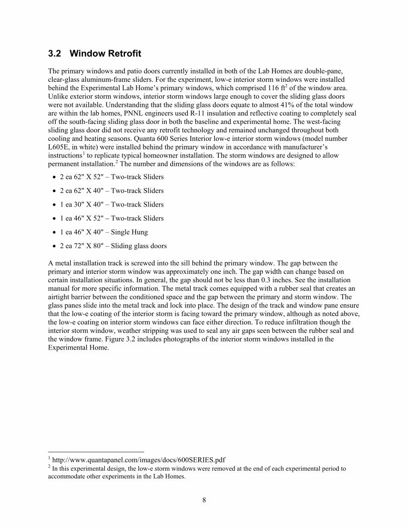
To help understand the dynamic flow of heat from the outside of the each home to inside, advanced metering techniques were used to catalog the temperature at differing points on both the primary and secondary glazing. Figure 3.3 displays the temperature measurements points that were placed on one window facing each cardinal direction, except east.
13
Figure 3.3. Interior Storm Window Temperature Measurement Points
All metering was completed using Campbell Scientific data loggers and matching sensors. Two Campbell data loggers were installed in each home, one allocated to electrical measurements and one to temperature and other data collection. Data from all sensors were collected via cellular modems that were individually connected to each of the loggers.
All data were captured at 1-minute intervals by the Campbell Scientific data loggers. These 1-minute data were averaged over hourly and daily time intervals to afford different analysis activities.
Occupancy in the homes was simulated via a programmable commercial lighting breaker panel (one per home) using motorized breakers. These breakers were programmed to activate connected loads on schedules to simulate human occupancy by introducing heat to the space.
Interior Storm Interior Surface Temperature
Existing Window Interior Surface Temperature
Interstitial Space Temperature
Existing Window Exterior Surface Temperature
Data logger for Space Temperatures
14
4.0 Results and Discussion
The air-leakage and HVAC energy performance of interior low-e storm window were evaluated during the 2015 heating season and cooling season in the PNNL Lab Homes. The subsequent sections provide a summary of the baseline performance of the two homes, as well as a comparison of the infiltration and energy usage of the Experimental Home equipped with interior low-e storm windows and the Baseline Home equipped with double-pane clear-glass windows and no attachments. Note that all experimental results are presented, in general, as daily averages with 95% confidence intervals calculated for each measured quantity, assuming a normal distribution of the data and applying a student’s t-statistic. The 95% confidence interval is then used to establish the significance of the differences observed as a result of the low-e storm window retrofit by applying a traditional significance test.
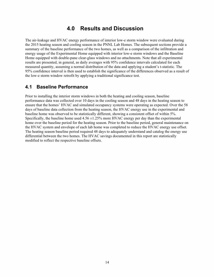
4.1 Baseline Performance
Prior to installing the interior storm windows in both the heating and cooling season, baseline performance data was collected over 10 days in the cooling season and 48 days in the heating season to ensure that the homes’ HVAC and simulated occupancy systems were operating as expected. Over the 58 days of baseline data collection from the heating season, the HVAC energy use in the experimental and baseline home was observed to be statistically different, showing a consistent offset of within 5%. Specifically, the baseline home used 4.56 ±1.25% more HVAC energy per day than the experimental home over the baseline period for the heating season. Prior to the baseline period, general maintenance on the HVAC system and envelope of each lab home was completed to reduce the HVAC energy use offset. The heating season baseline period required 48 days to adequately understand and catalog the energy use differential between the two homes. The HVAC savings documented in this report are statistically modified to reflect the respective baseline offsets.
15
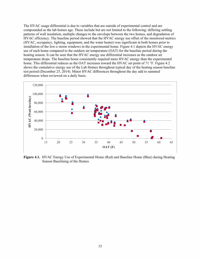
The HVAC usage differential is due to variables that are outside of experimental control and are compounded as the lab homes age. These include but are not limited to the following: differing settling patterns of wall insulation, multiple changes to the envelope between the two homes, and degradation of HVAC efficiency. The baseline period showed that the HVAC energy use offset of the monitored metrics (HVAC, occupancy, lighting, equipment, and the water heater) was significant in both homes prior to installation of the low-e storm windows in the experimental home. Figure 4.1 depicts the HVAC energy use of each home compared to the outdoor air temperature (OAT) for the baseline period during the heating season. It can be seen that the HVAC energy use differential increases as the outdoor air temperature drops. The baseline home consistently required more HVAC energy than the experimental home. This differential reduces as the OAT increases toward the HVAC set point of 71 °F. Figure 4.2 shows the cumulative energy use of the Lab Homes throughout typical day of the heating season baseline test period (December 25, 2014). Minor HVAC differences throughout the day add to summed differences when reviewed on a daily basis.
Figure 4.1. HVAC Energy Use of Experimental Home (Red) and Baseline Home (Blue) during Heating
Season Baselining of the Homes
0
20,000
40,000
60,000
80,000
100,000
120,000
15 20 25 30 35 40 45 50 55 60 65
HV
AC
(Wat
t-hr
s/da
y)
OAT (F)

16
Figure 4.2. Cumulative HVAC Energy Use of the Experimental Home (Red) and the Baseline Home
(Blue) throughout one day of the Baseline Period
4.2 Building Shell Air Leakage
Building shell air leakage in both Lab Homes was measured prior to the beginning of the experiment to obtain a baseline reading on the homes and ensure equivalent air-leakage performance between the two homes. Prior to the low-e storm windows installation, the blower door test1 results showed the air leakage of the two homes to be statistically the same, with 95% confidence. Accounting for experimental error in the blower door measurement and the blower door instrument accuracy, the baseline home had an air-leakage rate of 824 ±30.3 cfm at 50 Pa depressurization with respect to the outside (cfm50) and the experimental home had an air leakage of 869 ±26.9 cfm50.
After installation of the interior storm windows on the experimental home, the home was retested for air leakage. Results are tabulated in Table 4.1. These tests evaluate the relative leakiness of the primary window as compared to the storm window, to determine which window forms the primary air barrier for the home and suggest the relative contribution of each to any reduction in whole-house air leakage. Relative leakiness, particularly with interior storm windows, is extremely sensitive to installation process and sealing technique. Due to the fact that the interior storm window fits within the frame of the window sill, minimal inaccuracies in window measurements and unsquare window frames can cause gaps between the interior storm window track and the homes window sill. The storm window is equipped with a rubber gasket to help generate an air tight barrier. To ensure adequate sealing for the experimental period, internal weather stripping was used along the interior storm window track. This was not done in excess, but to the degree that a typical home owner might engage in.
1 Blower door testing equipment measures flow with an accuracy of ±3%. http://www.energyconservatory.com/products/automated-blower-door-systems-and-accessories
0
10,000
20,000
30,000
40,000
50,000
60,000
1 2 3 4 5 6 7 8 9 10 11 12 13 14 15 16 17 18 19 20 21 22 23 24
HV
AC
Ene
rgy
(Wat
t-hr
s)
Time

17
Table 4.1. Blower Door Test Results Pre and Post Storm Windows Installation
Parameter
Experimental Home Pre–Window Installation
Experimental Home Post–Window Installation
Average Value 95% Confidence
Interval Average Value 95% Confidence
Interval
cfm50(a) 869 26.9 846 26.2 ACH50 4.18 0.13 4.07 0.12 ACHn
(b) 0.19 0.01 0.18 0.01 (a) Cubic feet per minute at 50 Pascals depressurization (b) n = 21.5, based on single-story home in climate zone 3, with minimal shielding
The installation of the storm windows over 74% of the window area in the experimental home showed a minimal reduction in air leakage from 869.1 ±26.9 cfm50 to 846.1 ±26.2 cfm50, which is a 23.0 ±37 cfm50, or 2.6 ±4.2%, reduction. This is the change in air leakage for the entire Lab Home just from the addition of storm windows; no other air sealing measures were applied to the home. The decrease in air leakage is not statistically significant, with 95% confidence, because the error in the measurements is greater than the average difference between the measurements. This testing suggests that for the experimental home, the primary window remains the primary air barrier, and the closed storm window provides no statistically significant reduction in air leakage. However, it should be noted that the Lab Homes are relatively airtight at about 4 ACH50, whereas air leakage in older homes is commonly much higher. For homes that have leakier windows, installing interior storm windows could have a more significant impact on the air leakage than seen here.
Previous field studies have demonstrated significant reductions in air leakage from the application of storm windows. In a previous case study of five Chicago weatherization homes, an average 7% reduction in overall home air leakage was observed from the addition of exterior storm windows (Drumheller et al. 2007). In addition, an average 10% reduction in overall apartment air leakage was observed for a field study of low-e storm windows on two large apartment buildings in Philadelphia, and an average 17% average reduction in overall home air leakage was observed for storm windows used in 10 older weatherization homes near Atlanta (Quanta 2013). The reduction in air leakage observed in these case studies was greater than reductions observed in the experimental home, most likely due to the higher initial leakiness of the primary existing windows in these older buildings.
4.3 Low-E Storm Window Energy Performance
After retrofitting the experimental home with interior low-e storm windows experimental data was collected from July 24 to August 12, 2015, to characterize the energy and thermal performance of the windows during the cooling season, and from January 20 to February 16, 2015, to characterize performance during the heating season.
To compare and assess the performance of the interior storm windows relative to the baseline windows, HVAC energy use and interior and glass surface temperatures were compared on an average daily basis. This comparison shows significant HVAC energy savings in the Lab Home with the low-e storm windows installed (experimental home). The overall HVAC savings from installing interior storm panels over 74% of the window area in the experimental home are 8.1 ±1.9% in the heating season and 4.2 ±0.7% in the cooling season.
18
4.3.1 Winter Heating Season Results
Heating during the winter was provided solely by a forced-air electric resistance furnace. Although a variety of heating systems and fuel types are used in homes, using electric resistance heating allows precise direct measurement of thermal energy impact of the low-e storm windows in the Lab Home experiments, because the electric resistance elements are 100% efficient. These results can then be easily extrapolated to other heating system types based on the relative efficiency of those systems.
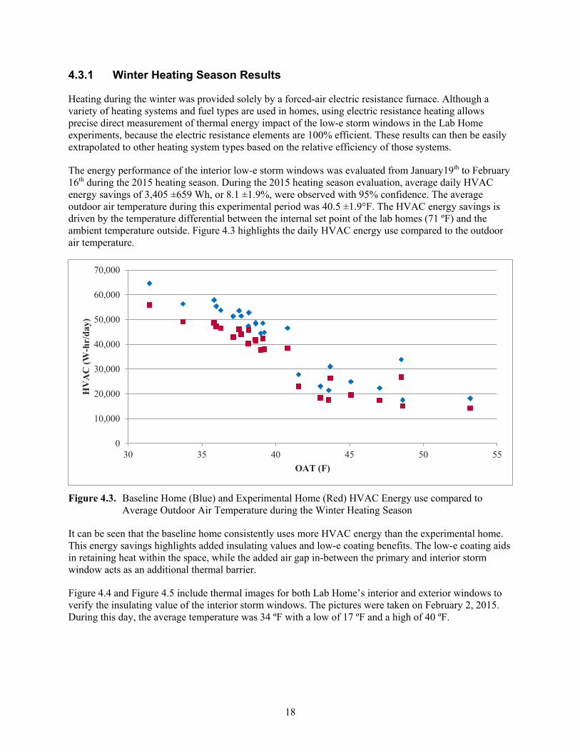
The energy performance of the interior low-e storm windows was evaluated from January19th to February 16th during the 2015 heating season. During the 2015 heating season evaluation, average daily HVAC energy savings of 3,405 ±659 Wh, or 8.1 ±1.9%, were observed with 95% confidence. The average outdoor air temperature during this experimental period was 40.5 ±1.9°F. The HVAC energy savings is driven by the temperature differential between the internal set point of the lab homes (71 ºF) and the ambient temperature outside. Figure 4.3 highlights the daily HVAC energy use compared to the outdoor air temperature.
Figure 4.3. Baseline Home (Blue) and Experimental Home (Red) HVAC Energy use compared to
Average Outdoor Air Temperature during the Winter Heating Season
It can be seen that the baseline home consistently uses more HVAC energy than the experimental home. This energy savings highlights added insulating values and low-e coating benefits. The low-e coating aids in retaining heat within the space, while the added air gap in-between the primary and interior storm window acts as an additional thermal barrier.
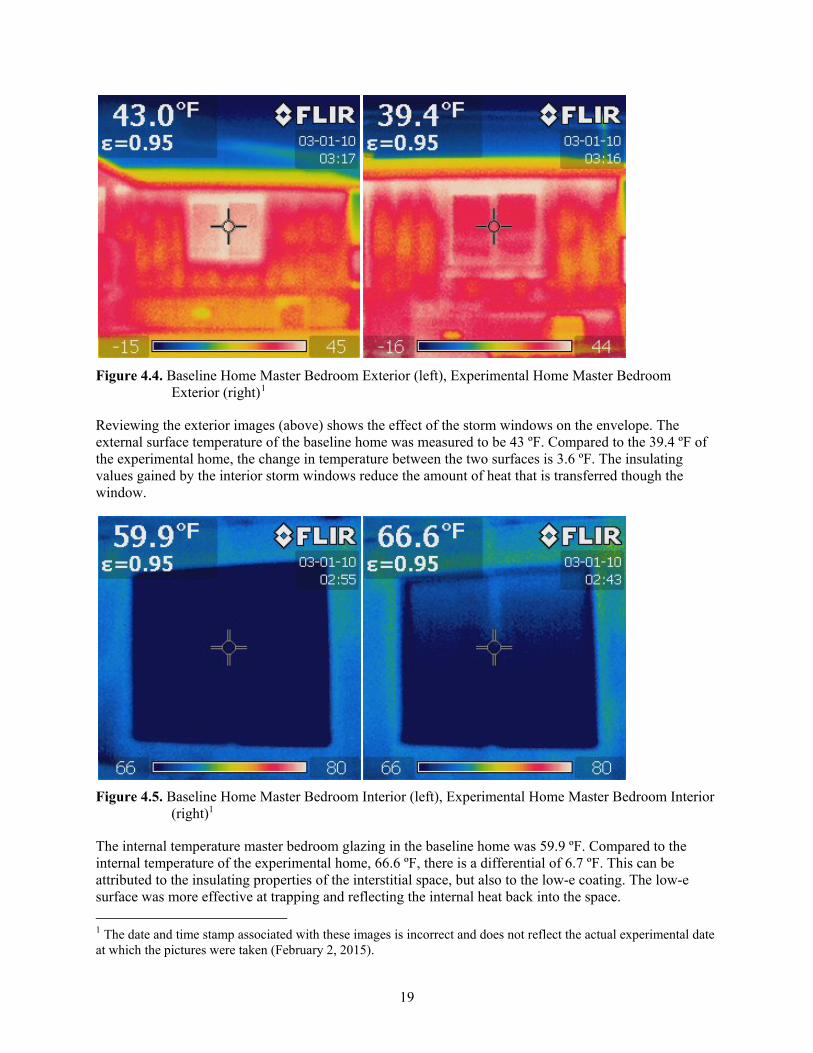
Figure 4.4 and Figure 4.5 include thermal images for both Lab Home’s interior and exterior windows to verify the insulating value of the interior storm windows. The pictures were taken on February 2, 2015. During this day, the average temperature was 34 ºF with a low of 17 ºF and a high of 40 ºF.
0
10,000
20,000
30,000
40,000
50,000
60,000
70,000
30 35 40 45 50 55
HV
AC
(W-h
r/da
y)
OAT (F)
19
Figure 4.4. Baseline Home Master Bedroom Exterior (left), Experimental Home Master Bedroom
Exterior (right)1
Reviewing the exterior images (above) shows the effect of the storm windows on the envelope. The external surface temperature of the baseline home was measured to be 43 ºF. Compared to the 39.4 ºF of the experimental home, the change in temperature between the two surfaces is 3.6 ºF. The insulating values gained by the interior storm windows reduce the amount of heat that is transferred though the window.
Figure 4.5. Baseline Home Master Bedroom Interior (left), Experimental Home Master Bedroom Interior
(right)1
The internal temperature master bedroom glazing in the baseline home was 59.9 ºF. Compared to the internal temperature of the experimental home, 66.6 ºF, there is a differential of 6.7 ºF. This can be attributed to the insulating properties of the interstitial space, but also to the low-e coating. The low-e surface was more effective at trapping and reflecting the internal heat back into the space. 1 The date and time stamp associated with these images is incorrect and does not reflect the actual experimental date at which the pictures were taken (February 2, 2015).

20
4.3.2 Summer Cooling Season Results
Cooling during the summer was provided by a 2.5-ton seasonal energy-efficiency ratio (SEER) 13 heat pump. During the cooling season the interior storm window installation over 74% of the window area resulted in a daily HVAC energy savings of 1,186 ±202 Wh, which is an 4.2 ±0.7% reduction in HVAC cooling energy use. These savings are primarily due to two main factors. The first is the increased insulating of the additional pane of glass and the added interstitial air space. The second is a reduction in the solar heat gain from the low-e storm windows. The HVAC energy savings associated with these factors is dependent on the temperature differential between the internal set point of the Lab Homes and the ambient air temperature. Figure 4.6 displays the daily peak outdoor temperature and the percent daily HVAC energy savings.
Figure 4.6. Percent HVAC Energy Savings compared to Peak outdoor air temperature over the Summer
Cooling Season
Figure 4.6 highlights the trend of decreasing HVAC energy savings as peak outdoor temperature increases. As the ambient temperature increases, the effect of the low-e coating or interior storm windows decreases. One theory is that with rising temperatures and a window to wall ratio of just over 15%, the thermal gains associated with the envelope begin to dominate and almost nullify the savings associated with the interior storm windows. In addition, because interior low-e storm windows were not available to cover the sliding doors, only 30% of west-facing window area in the experimental home is covered with low-e storm panels. Due to the fact that these interior storm windows are optimized for colder climates and not all windows are covered with low-e storm windows, the HVAC savings during the cooling season is reduced.
4.3.3 Temperature Profile
To better understand how the additional low-E pane and interstitial space affected window assembly heat transfer, time-series surface temperature graph profiles were developed. The first profile, Figure 4.8, presents the exterior surface temperatures (and outside air temperature) for the same window in both Lab Homes. The data presented are for Thursday, January 29, 2015, an overcast day (no direct sunlight) with an average outside air temperature of just under 40 °F.
0.0%
1.0%
2.0%
3.0%
4.0%
5.0%
6.0%
7.0%
8.0%
80 85 90 95 100 105
Perc
ent H
VA
C S
avin
gs
Peak OAT (F)

21
Of note in the figure, the surface temperature for the baseline home, shown in blue, is estimated to be 5–6 ˚F warmer than the experimental home surface temperature, shown in green. A better insulating window assembly (additional window pane, low-E coating, and insulating air gap) helps to reduce the heat transfer between the conditioned space and the outside. The net result of this better performance is a cooler outside surface temperature for the improved window assembly – as shown in the graph (Experimental Home B and green line) and confirmed with the IR image (Figure 4.4).
Figure 4.7. Temperature comparison of exterior window glass between Baseline Home A (Blue) and
Experimental Home B (Green) During the Heating Season
Figure 4.9 compiles the relevant surface and interstitial temperatures for the same two windows. This figure starts with the outside air temperature (red series), and then presents the inside surface temperature of the experimental home’s existing double pane window (light blue). The next series (green) presents the experimental home’s window interstitial space temperature; this is the air temperature between the existing double pane window and the new interior storm window. The next series (darker blue) presents the baseline home’s inside surface temperature. This surface faces the occupied space of the baseline home and is the temperature felt by occupants. The final series (purple) is the interior surface temperature of the low-e storm window in the baseline home.
Evident from Figure 4.9 is the relatively warmer inside surface temperature of the experimental home’s low-e window versus the baseline home’s existing double pane window. This difference, varying between 4–6 ˚F, results in reduced heat transfer and improved thermal comfort.

22
Figure 4.8. Temperature Surface Gradient between Baseline Home (Lab A) and Experimental Home
(Lab B) During the Heating Season
4.3.4 Dependence on Outdoor Air Temperature and Solar Insolation
Savings were also analyzed with respect to daily weather variation, including outdoor air temperature and degree of cloud cover. In both the cooling and the heating season, the magnitude of HVAC energy savings showed significant dependence on these weather attributes.
HVAC energy use of the baseline and experimental homes both show a dependence on outdoor air temperature, as shown in Figure 4.10. A relationship between HVAC energy use and the outdoor air temperature is expected because the temperature difference between the inside and outside is the primary driver for HVAC energy use. In Figure 4.10, the baseline home (blue diamonds) exhibits slightly greater average energy use (higher points) than the experimental home (red squares). The data also shows greater temperature dependence of heating season energy use versus cooling season energy use. This is expected because of the lower efficiency of the forced-air electric resistance heating system compared to the heat pump cooling system. The percent savings within the graph is higher than reported because the baseline offset is not taken into account within this graph.
23
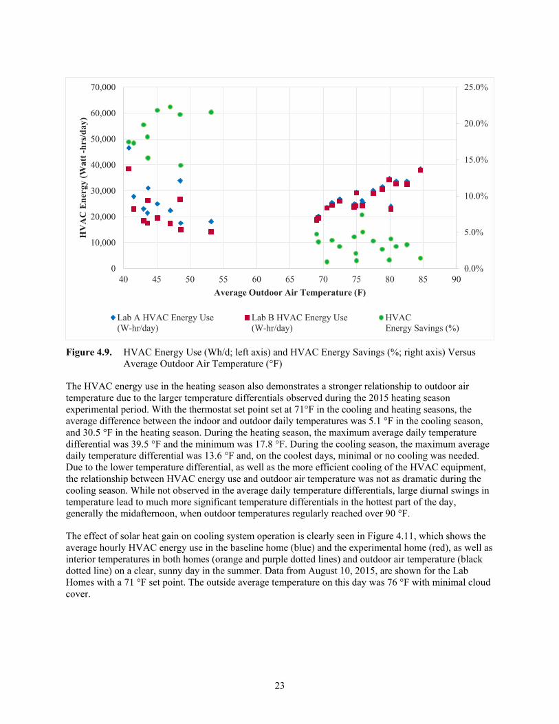
Figure 4.9. HVAC Energy Use (Wh/d; left axis) and HVAC Energy Savings (%; right axis) Versus
Average Outdoor Air Temperature (°F)
The HVAC energy use in the heating season also demonstrates a stronger relationship to outdoor air temperature due to the larger temperature differentials observed during the 2015 heating season experimental period. With the thermostat set point set at 71°F in the cooling and heating seasons, the average difference between the indoor and outdoor daily temperatures was 5.1 °F in the cooling season, and 30.5 °F in the heating season. During the heating season, the maximum average daily temperature differential was 39.5 °F and the minimum was 17.8 °F. During the cooling season, the maximum average daily temperature differential was 13.6 °F and, on the coolest days, minimal or no cooling was needed. Due to the lower temperature differential, as well as the more efficient cooling of the HVAC equipment, the relationship between HVAC energy use and outdoor air temperature was not as dramatic during the cooling season. While not observed in the average daily temperature differentials, large diurnal swings in temperature lead to much more significant temperature differentials in the hottest part of the day, generally the midafternoon, when outdoor temperatures regularly reached over 90 °F.
The effect of solar heat gain on cooling system operation is clearly seen in Figure 4.11, which shows the average hourly HVAC energy use in the baseline home (blue) and the experimental home (red), as well as interior temperatures in both homes (orange and purple dotted lines) and outdoor air temperature (black dotted line) on a clear, sunny day in the summer. Data from August 10, 2015, are shown for the Lab Homes with a 71 °F set point. The outside average temperature on this day was 76 °F with minimal cloud cover.
0.0%
5.0%
10.0%
15.0%
20.0%
25.0%
0
10,000
20,000
30,000
40,000
50,000
60,000
70,000
40 45 50 55 60 65 70 75 80 85 90
HV
AC
Ene
rgy
(Wat
t -hr
s/da
y)
Average Outdoor Air Temperature (F)
Lab A HVAC Energy Use(W-hr/day)
Lab B HVAC Energy Use(W-hr/day)
HVACEnergy Savings (%)

24
Figure 4.10. HVAC Energy Use and Indoor Temperature for the Experimental Home (red and purple
lines) and the Baseline Home (blue and orange lines) on a Warm, Sunny Day (8/10/2015)
During the night, the Lab Homes had similar cooling HVAC characteristics due to the fact that the outdoor temperature hovered around the internal set point of the homes. Sunrise occurred between 5 and 6 a.m., and the cooling load dropped as the homes began to warm towards their balance point. Increased outdoor air temperature steadily increased the HVAC energy cooling load throughout the morning as the envelope of the homes began to heat. Solar heat gains became a factor at about 11 a.m. as the solar intensity increased and the homes continued to warm up. The smoothing in the experimental home (red) peak HVAC energy use between 11 a.m. and 3 p.m. can be attributed to the installation of the low-e interior storm windows and their effect on the U-factor and SHG of the space. The effectiveness of the windows was minimized as the increased solar gains of the envelope drove the systems in both homes to operate similarly between 3 p.m. and 7 p.m. Also, because interior low-e storm windows were not available to cover the sliding doors, only 30% of west-facing window area in Lab Home B is covered with low-e storm panels, and the two homes will have similar higher solar gains on the west side in the afternoon through the large door. Additional HVAC cooling savings were achieved as dusk approached and the homes began to cool. The west-facing windows1 reflected some of the solar radiation and reduced the cooling load from 6 p.m. to 9 p.m. Post-sunset, the homes began to cool toward the HVAC set point, where they remained until dawn the following day. Figure 4.12 shows the cumulative HVAC energy use on 8/10/2015. As shown in the previous graph, the performance of the HVAC systems remained similar until the envelope and outdoor air temperature began to increase. Solar heat gains drove the increased HVAC energy usage for the baseline home compared to the experimental home.
1 Where only 30% of the west-facing window area in Lab Home B is covered with a low-e storm window.
0
10
20
30
40
50
60
70
80
90
100
0
500
1,000
1,500
2,000
2,500
3,000
1 2 3 4 5 6 7 8 9 10 11 12 13 14 15 16 17 18 19 20 21 22 23 24Time
Tem
pera
ture
(F)
HV
AC
(Wat
t -hr
s)
Baseline HVAC Experimental HVAC OAT
Baseline Indoor Temp Experimental Indoor Temp

25
Figure 4.11. Cumulative HVAC Energy Use of the Experimental Home (Red) and Baseline Home
(Blue) on a typical day during the Cooling Season
A different effect can be seen during the heating season experiments. The effect of solar heat gain on heating system operation is seen in Figure 4.13, which shows the average hourly HVAC energy use in the baseline home (blue) and the experimental home (red), as well as interior temperatures in both homes (orange and purple dotted lines) and outdoor air temperature (black dotted line) on a clear, sunny day in the winter. Data from February 11, 2015, are shown for the Lab Homes with a 71 °F set point. The outside average temperature on this day was 45 °F with minimal cloud cover.
0
5,000
10,000
15,000
20,000
25,000
30,000
1 2 3 4 5 6 7 8 9 10 11 12 13 14 15 16 17 18 19 20 21 22 23 24
HV
AC
Ene
rgy
(Wat
t-hr
s)
Time

26
Figure 4.12. HVAC Energy Use and Indoor Temperature for the Experimental Home (red and purple lines) and the Baseline Home (blue and orange lines) on a Sunny Day (2/11/2015)
During the morning, the experimental home showed decreased HVAC energy use when compared to the baseline home due to the reduced heat loss resulting from the addition of low-e storm windows. The cooler outdoor temperature caused a majority of the heating load to take place during the morning hours of the day. At about midday, the solar heat gains increased the internal temperature above the set point and were sufficient enough to reduce the heating load to zero for the remainder of the afternoon. At 9 p.m., the internal temperature of the baseline home decreased below the set point and heating was required. The insulating properties of the low-e coating keep the baseline home at an increased internal temperature throughout the evening. This causes the heating load to shift by about one hour when compared to the baseline home.
Figure 4.14 details the cumulative HVAC energy use over February 11, 2015. The initial load shift of the morning heating event can be seen within the graph. This shift adds an offset to the cumulative distribution. Initially, the baseline home required heating sooner than the experimental home. The peak reduction in HVAC energy use throughout the experimental period increased the energy savings and distance between the two lines.
0
10
20
30
40
50
60
70
80
0
500
1,000
1,500
2,000
2,500
3,000
3,500
1 2 3 4 5 6 7 8 9 10 11 12 13 14 15 16 17 18 19 20 21 22 23 24
Tem
pera
ture
(F)
HV
AC
(Wat
t -hr
s)
TimeExperimental HVAC Baseline HVAC OAT
Baseline Indoor Temp Experimental Indoor Temp

27
Figure 4.13. Cumulative Energy Use of the Experimental Home (Red) Versus the Baseline Home (Blue)
during the Heating Season
The difference in solar insolation transmitted through the glass of the west-facing window in the baseline home and corresponding window in the experimental home can partially be seen in Figure 4.15. There is a direct relationship between the amount of solar insolation that is absorbed and the percent of HVAC energy savings demonstrated by the experimental over the baseline home. The reduction in the SHGC effects the solar heat transmitted to the building though conduction, convection, or radiation.
Figure 4.14. Percent HVAC Energy Savings Compared to Measured Solar Insolation
0
5,000
10,000
15,000
20,000
25,000
30,000
1 2 3 4 5 6 7 8 9 10 11 12 13 14 15 16 17 18 19 20 21 22 23 24
HV
AC
Ene
rgy
(Wat
t-hr
s)
Time
0.0%
5.0%
10.0%
15.0%
20.0%
25.0%
0 5 10 15 20 25 30
HV
AC
Ene
rgy
Savi
ngs
Difference in Solar Insolation between the Lab Homes (MJ/m2)

28
4.4 Average Annual Savings
An EnergyPlus model was created for the Lab Homes to compare modeled HVAC energy savings from the installation of interior low-e storm windows over 74% of the window area in the experimental home to the measured results from the experiment. The EnergyPlus analysis shows an average HVAC energy savings in the experimental home from the low-e storm panels to be 8.2% during the heating season experimental period. The modeled results correspond well with the measured data of 8.1 ±1.9% HVAC energy savings. For the cooling season, the measured data reflected a 4.2 ±0.7% savings during the experimental time period.
To extrapolate annual energy savings from the seasonal measured data, EnergyPlus simulations were used with adjustments to reflect observed load profiles and onsite weather data. The modeled annual energy savings from the installation of low-e storm panels over approximately 74% of the window area in Lab Home B was 7.8% or 1,006 kWh/yr, with a cooling and heating set point of 71ºF.
4.5 Interior Temperature Distributions
As expected, the interior storm windows also had some impact on indoor temperature distribution within the homes. Indoor temperatures for differing rooms in each home, the average interior temperature, and the thermostat set point are shown in Figure 4.16 and Figure 4.17 for the heating season and cooling season, respectively. Comparing the temperature profiles of the Lab Homes on a sunny day in the heating season (Figure 4.16), one can see that the experimental home experiences increased thermal capacity and remains warmer into the evening than the baseline home. Though this seems to be a minimal effect, it is more than likely due to the installation of the interior storm windows.
Figure 4.17 shows overcooling occurring in some rooms in both homes during the cooling season, probably due to the location of the thermostat (in the hallway adjacent to the kitchen in both homes). Temperatures between 60°F and 62°F are observed in both Lab Homes A and B in the rooms closest to the air handler—the bathroom, west bedroom, and east bedroom receive the most air because of shorter duct runs.

29
Figure 4.15. Interior Temperature Distribution for Lab Home A (left) and Lab Home B (right) on 2/15/215, a Sunny Day in the Heating Season

30
Figure 4.16. Interior Temperature Distribution for Lab Home A (left) and Lab Home B (right) on 8/11/2015, a Hot Sunny Day in the Cooling
Season

31
5.0 Interior and Exterior Storm Window Comparison
In 2014, PNNL conducted an evaluation of exterior storm windows during the heating and cooling seasons within the Lab Homes (Knox and Widder 2014). The study quantified the estimated annual whole house energy savings based on data collected during the cooling and heating season and the reduction in infiltration rates due to the exterior storm window retrofit. The HVAC technology implemented in the cooling season was a 2.5-ton seasonal energy-efficiency ratio (SEER) 13 heat pump. During the heating season, the heat pump was disabled and a forced-air electric resistance furnace supplied the required heating to the Lab Homes. In general, measured HVAC savings due to the exterior storm windows averaged 10.5% for the heating season and 8.0% for the cooling season for identical occupancy conditions. Extrapolating these energy savings numbers based on typical average heating degree days and cooling degree days per year yields an estimated annual energy savings of 10.1%, or 2,216 kWh/yr (Knox and Widder 2014).
During the evaluation of the interior storm windows, the same HVAC technology was implemented. Differing experimental parameters (e.g., differing window-to-wall ratios and differing coverage of low-e storm windows) and variable outdoor air temperatures maximized the annual savings within the exterior storm windows experiment and minimized the savings during interior storm windows experiment. Though the magnitude of the savings differ, the percentage savings are similar.
During the exterior storm windows heating season, a large temperature delta was implemented by setting the interior set point to 75°F. The increased internal set point coupled with unseasonably cold heating season temperatures (average outdoor air temperature of 28.3°F) drove the temperature delta to 46.7°F between the interior of the space and average OAT. In comparison, the internal set point of the interior storm windows experiment was 71°F with an average outdoor air temperature of 40.5°F during the heating season experimental period. The temperature delta seen is 30.5°F. The 16.2°F temperature differences between the two experiments greatly influenced the heating energy savings and subsequently, the estimated annual energy. In addition, the difference in the window-to-wall ratio from the coverage of 40 ft2 of window area (one of the sliding glass doors) reduced the overall heating and cooling load for the homes during the interior storm window experiments, which reduced the overall energy savings in terms of kilowatt hours.
Finally, the difference in window area coverage by low-e storm windows appears to have influenced the percentage savings when comparing the storm window experiments. Where the exterior low-e storm window experiments had low-e storm windows installed over 100% of the window area, the interior low-e experiments only covered 74% of the window area with low-e storm panels. Thus, based on the comparison of results from the two experiments, it could be concluded that to achieve the full benefit of the low-e interior storm window, complete coverage of all of the window area is recommended. It has been shown that partial coverage is beneficial and can save on HVAC energy, but complete coverage would have increased the shown savings.

32
6.0 Conclusions
This experiment used two side-by-side Lab Homes on the PNNL campus to measure the potential energy savings impacts of interior low-e storm windows in the Experimental Home compared to the baseline home equipped with standard double-pane clear-glass, aluminum-frame windows. The windows in the baseline home are representative of many existing homes across the Pacific Northwest and much of the United States. Testing was conducted during the 2014–2015 winter heating and 2015 summer cooling seasons and the collected data showed that interior low-e storm windows installed over 74% of the window area in Lab Home B resulted in an 8.1 ±1.9% and 4.2 ± 0.7% reduction in HVAC energy use during the heating and cooling season, respectively. Using EnergyPlus, the annualized HVAC energy savings equated to 7.8% or 1,006 kWh/yr.
This evaluation has added to the body of knowledge about low-e storm windows by presenting measureable energy savings in a controlled setting. Results from this study clearly show that low-e storm windows are viable energy retrofits in single-family residences and should be explored further across a variety of building types and climate zones.

33
7.0 References
AAMA (American Architectural Manufacturers Association). 2012. “Window and Door Sales to Accelerate Next Year.” Window & Door Magazine. Volume 20, Number 4, June/July 2012, – American Architectural Manufacturers Association.
Baylon, D, P Storm, B Hannas, K Geraghty, and V Mugford. 2013. Residential Building Stock Assessment: Multifamily Characteristics and Energy Use. Ecotope (September 5, 2013), Report #13-263, sponsored by Northwest Energy Efficiency Alliance and available online: http://neea.org/docs/default-source/reports/residential-building-stock-assessment--multi-family-characteristics-and-energy-use.pdf?sfvrsn=4.
Cort KA. 2013. Low-E Storm Windows: Market Assessment and Pathways to Market Transformation. PNNL-22565, Pacific Northwest National Laboratory, Richland, Washington.
Culp TD, and KA Cort. 2014. Database of Low-E Storm Window Energy Performance across U.S. Climate Zones . PNNL-22864, Rev. 2. Pacific Northwest National Laboratory, Richland, Washington.
Culp TD, SC Drumheller, and J Wiehagen. 2015. Low-E Retrofit Demonstration and Education Program. Final Report, U.S. DOE project #DE-E E0004015, Quanta Technologies, Malvern, Pennsylvania.
Culp TD, SH Widder, and KA Cort. 2015. Thermal and Optical Properties of Low-E Storm Windows and Panels . PNNL-24444, Pacific Northwest National Laboratory, Richland, WA.
Curcija DC, M Yazdanian, et al. 2013. Energy Savings from Window Attachments. Prepared for U.S. Department of Energy under DOE EERE award #DE-FOA-0001000. Lawrence Berkeley National Laboratory, Berkeley, California
Drumheller SC, C Kohler, and S Minen. 2007. Field Evaluation of Low-e Storm Windows. LBNL 1940E, Lawrence Berkley National Laboratory, Berkeley, California.
Energy Information Administration (EIA). 2014. Electric Power Monthly. Available at: http://www.eia.gov/electricity/monthly/epm_table_grapher.cfm?t=epmt_5_3
Huang, J, J Hanford, et al. 1999. Residential Heating and Cooling Loads Component Analysis. LBNL-44636, Building Technologies Department, Lawrence Berkeley National Laboratory, Berkeley, California.
Klems JH. 2003. “Measured Winter Performance of Storm Windows.” ASHRAE Transactions 109(2), Paper KC-03-12-1, Lawrence Berkeley National Laboratory, Berkeley, California.
Knox, JR and SH Widder. 2014. Evaluation of Low-e Storm Windows in the PNNL Lab Homes. PNNL-23355, May 2014. Pacific Northwest National Laboratory, Richland, Washington. Available online at: http://labhomes.pnnl.gov/documents/PNNL_23355_Lab_Homes_Low-e_Storms.pdf.
Krigger J and B Van der Meer. 2011. Weatherization Standards and Field Guide for Pennsylvania. Published for the U.S. Department of Energy Weatherization Assistance Program and the Pennsylvania Department of Community, Economic Development, and Office of Energy Conservation and Weatherization, Harrisburg, Pennsylvania.
34
Navigant Consulting. 2014. 2014 Commercial Building Stock Assessment: Final Report. December 16, 2014. Sponsored by the Northwest Energy Efficiency Alliance. Available online: http://neea.org/resource-center/regional-data-resources/commercial-building-stock-assessment.
Parker GB, TS Mapes, and WJ Zalis. 2013. Highly Insulating Windows Volume Purchase Program Final Report. PNNL-22183, DOE/EE-0884, Pacific Northwest National Laboratory, Richland, Washington.
Quanta Technologies. 2013. 2012-13 Quarterly Reports prepared for U.S. Department of Energy under DOE EERE award #DE-EE0004015, Malvern, Pennsylvania.
Widder SW, MC Baechler, et al. 2012. Side-by-Side Field Evaluation of Highly Insulating Windows in the PNNL Lab Homes. PNNL-21678, Pacific Northwest National Laboratory, Richland, Washington.
Zalis W, et al. 2010 Evaluation of Low-E Storm and R-5 Windows for Inclusion in Pennsylvania’s Weatherization Priority List. Prepared by W Zalis, Energetics; Culp, Birch Point Consulting; C Kohler, LBNL; and PM LaFrance, U.S. Department of Energy; for the Pennsylvania Department of Community and Economic Development,, Columbia, Maryland.

1

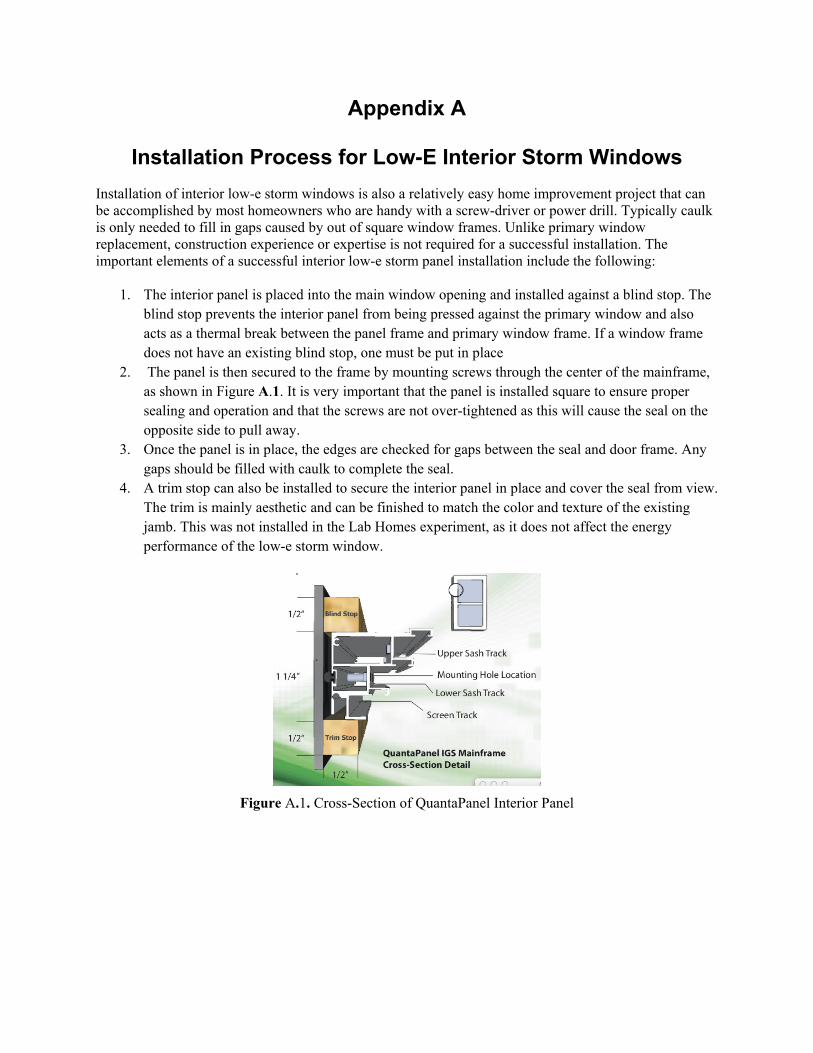
Appendix A –
Installation Process for Low-E Interior Storm Windows Installation of interior low-e storm windows is also a relatively easy home improvement project that can be accomplished by most homeowners who are handy with a screw-driver or power drill. Typically caulk is only needed to fill in gaps caused by out of square window frames. Unlike primary window replacement, construction experience or expertise is not required for a successful installation. The important elements of a successful interior low-e storm panel installation include the following:
1. The interior panel is placed into the main window opening and installed against a blind stop. The blind stop prevents the interior panel from being pressed against the primary window and also acts as a thermal break between the panel frame and primary window frame. If a window frame does not have an existing blind stop, one must be put in place
2. The panel is then secured to the frame by mounting screws through the center of the mainframe, as shown in Figure A.1. It is very important that the panel is installed square to ensure proper sealing and operation and that the screws are not over-tightened as this will cause the seal on the opposite side to pull away.
3. Once the panel is in place, the edges are checked for gaps between the seal and door frame. Any gaps should be filled with caulk to complete the seal.
4. A trim stop can also be installed to secure the interior panel in place and cover the seal from view. The trim is mainly aesthetic and can be finished to match the color and texture of the existing jamb. This was not installed in the Lab Homes experiment, as it does not affect the energy performance of the low-e storm window.
Figure A.1. Cross-Section of QuantaPanel Interior Panel
