evaluation of modeling environments for managing ... · evaluation of modeling environments for...

Evaluation of Modeling Environments for managing Diagnostic Information

O S K A R F R A N K E

Master of Science Thesis Stockholm, Sweden 2009

Evaluation of Modeling Environments for managing Diagnostic Information

O S K A R F R A N K E

Master’s Thesis in Computer Science (30 ECTS credits) at the School of Computer Science and Engineering Royal Institute of Technology year 2009 Supervisor at CSC was Kjell Lindqvist Examiner was Lars Kjelldahl TRITA-CSC-E 2009:092 ISRN-KTH/CSC/E--09/092--SE ISSN-1653-5715 Royal Institute of Technology School of Computer Science and Communication KTH CSC SE-100 44 Stockholm, Sweden URL: www.csc.kth.se

Abstract

Scania is a leading manufacturer of heavy duty vehicles and buses aswell as industrial and marine engines.

In the vehicles there are software that implements a number of dif-ferent tests of sensors and actuators, as part of a diagnostic system.Since each sensor or actuator can be monitored by several tests, there isa need to isolate which of the sensors that are broken. To achieve this,a fault isolation algorithm is used. The fault isolation problem can bedescribed as a Constraint satisfaction problem (CSP).

This thesis presents the framework F-JOB diagnosis framework.The framework covers the complete sequence from modeling the sys-tem, with respect to fault isolation, to providing a valid diagnosis at theon-board system in the vehicle using a CSP solver. The CSP solver isnot implemented in this thesis. It is described in Johan Björling’s thesiscarried out in parallel on the same department as this was.

In this thesis a prototype has been implemented in Generic ModelingEnvironment, by first specifying a meta model for diagnostic informationand then using this meta model to create a model for different faultisolation problems.

The work also includes a comparison of the modeling environmentsGeneric Modeling Environment and Topcased. The comparison is basedon the Scania requirements for modeling environments.

Keywords: diagnosis, fault isolation, data modeling.

Referat

Utvärdering av modelleringsmiljöer för att hantera

diagnosinformation

Scania är en ledande tillverkare av tunga lastbilar, bussar samt industri-och marinmotorer.

I fordonen finns mjukvara som implementerar ett antal olika tes-ter av sensorer och aktuatorer som en del av ett diagnostiskt system.Eftersom varje sensor eller aktuator kan övervakas av flera tester, be-höver man, efter att testerna körts, isolera fram vilken eller vilka avsensorerna som är trasig. För detta används en felisoleringsalgoritm.Felisoleringsproblemet går att beskriva som ett Constraint satisfactionproblem (CSP).

Detta examensarbete presenterar F-JOB diagnosis framework. Ram-verket täcker alla delar från grafisk modellering, med avseende på feliso-lering, till diagnos on-board i fordonet med hjälp av en CSP-lösare. CSP-lösaren som används är inte implementerad inom detta examensarbete.Den beskrivs i Johan Björlings examensarbete som utförts parallellt påsamma avdelning.

En prototyp har implementerats i Generic Modeling Environment(GME) genom att först specificera en metamodell för diagnosinforma-tion och sedan, med hjälp av metamodellen, modellera olika felisole-ringsproblem. Prototypen tillsammans med ramverket exemplifierar hurScania kan arbeta med verktyg som exempelvis GME.

I arbetet finns också en jämförelse av modelleringeringsmiljöernaGME och Topcased. Jämförelsen grundar sig på krav som Scania ställerpå modelleringsmiljöer.

Nyckelord: diagnos, felisolering, datamodellering.

Preface

This is my master thesis work in my education aiming for a M.Sc. Computer Sciencedegree. The work has been performed at the diagnosis group under the departmentof Powertrain control systems at Scania in Södertälje and KTH School of ComputerScience and Communication from November 2008 to June 2009. Scania is a leadingmanufacturer of heavy duty vehicles and buses as well as industrial and marineengines.

First of all I would like to give a special thanks to my supervisor at Scania;Ph.D. Jonas Biteus, my supervisor at KTH; Kjell Lindqvist and my co-worker atScania, Johan Björling.

I would also like to thank all the participants in our reference group; MattiasNyberg, Tony Lindgren, Carl Svärd, Ulf Bergman and Lars Bergström.

Thanks to my family and especially my brother Ulrik for great help with struc-ture of the report and support during this project. Also Anna Kullberg and NickolinaKrajisnik deserves a special thank for their friendship.

Södertälje, June 2009Oskar Franke

Contents

1 Introduction 11.1 Background . . . . . . . . . . . . . . . . . . . . . . . . . . . . . . . . 1

1.2 Problem definition . . . . . . . . . . . . . . . . . . . . . . . . . . . . 11.3 Objective . . . . . . . . . . . . . . . . . . . . . . . . . . . . . . . . . 11.4 Strategy . . . . . . . . . . . . . . . . . . . . . . . . . . . . . . . . . . 21.5 Target group . . . . . . . . . . . . . . . . . . . . . . . . . . . . . . . 2

1.6 Related work . . . . . . . . . . . . . . . . . . . . . . . . . . . . . . . 21.7 Contributions . . . . . . . . . . . . . . . . . . . . . . . . . . . . . . . 21.8 Thesis outline . . . . . . . . . . . . . . . . . . . . . . . . . . . . . . . 3

2 The F-JOB diagnosis framework 52.1 Advantages . . . . . . . . . . . . . . . . . . . . . . . . . . . . . . . . 52.2 Parts of the F-JOB diagnosis framework . . . . . . . . . . . . . . . . 6

3 Background to model based fault diagnosis 73.1 Models . . . . . . . . . . . . . . . . . . . . . . . . . . . . . . . . . . . 73.2 Models for diagnosis . . . . . . . . . . . . . . . . . . . . . . . . . . . 8

3.2.1 Components and behavioral modes . . . . . . . . . . . . . . . 8

3.2.2 Observations . . . . . . . . . . . . . . . . . . . . . . . . . . . 83.2.3 Example . . . . . . . . . . . . . . . . . . . . . . . . . . . . . . 9

3.3 Diagnosis definitions . . . . . . . . . . . . . . . . . . . . . . . . . . . 93.4 A diagnosis system . . . . . . . . . . . . . . . . . . . . . . . . . . . . 10

3.4.1 Diagnostic tests . . . . . . . . . . . . . . . . . . . . . . . . . . 113.4.2 Fault isolation . . . . . . . . . . . . . . . . . . . . . . . . . . 11

4 Background to constraint satisfaction problems 15

4.1 Definition of CSP . . . . . . . . . . . . . . . . . . . . . . . . . . . . . 154.2 Definition of Weighted CSP (wCSP) . . . . . . . . . . . . . . . . . . 174.3 Model notation for CSP . . . . . . . . . . . . . . . . . . . . . . . . . 174.4 Outline of CSP-solver . . . . . . . . . . . . . . . . . . . . . . . . . . 18

4.5 Labelling Tree . . . . . . . . . . . . . . . . . . . . . . . . . . . . . . . 20

5 Background to meta models 215.1 Introduction . . . . . . . . . . . . . . . . . . . . . . . . . . . . . . . . 21

5.2 Model-driven engineering . . . . . . . . . . . . . . . . . . . . . . . . 21

5.3 Meta-Object Facility . . . . . . . . . . . . . . . . . . . . . . . . . . . 22

5.4 Some major modeling languages . . . . . . . . . . . . . . . . . . . . 22

6 Requirements for modeling environments 25

6.1 Introduction . . . . . . . . . . . . . . . . . . . . . . . . . . . . . . . . 25

6.2 Requirements . . . . . . . . . . . . . . . . . . . . . . . . . . . . . . . 25

6.2.1 Functional requirements . . . . . . . . . . . . . . . . . . . . . 25

6.2.2 Non-functional requirements . . . . . . . . . . . . . . . . . . 26

7 Assessment of modeling environments 27

7.1 Introduction . . . . . . . . . . . . . . . . . . . . . . . . . . . . . . . . 27

7.2 Tools used for modeling . . . . . . . . . . . . . . . . . . . . . . . . . 27

7.2.1 GME . . . . . . . . . . . . . . . . . . . . . . . . . . . . . . . 27

7.2.2 Topcased . . . . . . . . . . . . . . . . . . . . . . . . . . . . . 27

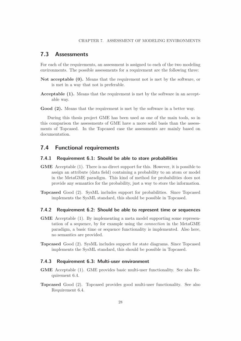
7.3 Assessments . . . . . . . . . . . . . . . . . . . . . . . . . . . . . . . . 28

7.4 Functional requirements . . . . . . . . . . . . . . . . . . . . . . . . . 28

7.4.1 Requirement 6.1: Should be able to store probabilities . . . . 28

7.4.2 Requirement 6.2: Should be able to represent time or sequences 28

7.4.3 Requirement 6.3: Multi-user environment . . . . . . . . . . . 28

7.4.4 Requirement 6.4: Support for revision control . . . . . . . . . 29

7.5 Non-functional requirements . . . . . . . . . . . . . . . . . . . . . . . 29

7.5.1 Requirement 6.5: Supported standards . . . . . . . . . . . . . 29

7.5.2 Requirement 6.6: Existing external support, still being devel-oped . . . . . . . . . . . . . . . . . . . . . . . . . . . . . . . . 29

7.5.3 Requirement 6.7: License type . . . . . . . . . . . . . . . . . 29

7.5.4 Requirement 6.8: Well-known by engineers . . . . . . . . . . 29

7.6 Summary . . . . . . . . . . . . . . . . . . . . . . . . . . . . . . . . . 30

8 Creating a meta model for fault isolation 31

8.1 Requirements for the fault isolation meta model . . . . . . . . . . . . 31

8.2 Meta model formalized in GME . . . . . . . . . . . . . . . . . . . . . 33

8.2.1 MetaGME . . . . . . . . . . . . . . . . . . . . . . . . . . . . . 33

8.2.2 Creating model using MetaGME . . . . . . . . . . . . . . . . 34

9 Implementation of fault isolation models 37

9.1 Introduction . . . . . . . . . . . . . . . . . . . . . . . . . . . . . . . . 37

9.2 A small fault isolation model . . . . . . . . . . . . . . . . . . . . . . 37

9.3 A fault isolation model for the Scania retarder . . . . . . . . . . . . 38

9.4 BON components . . . . . . . . . . . . . . . . . . . . . . . . . . . . . 38

9.4.1 Import data from database . . . . . . . . . . . . . . . . . . . 39

9.4.2 Priority of behavioral modes . . . . . . . . . . . . . . . . . . 39

9.4.3 Known bugs . . . . . . . . . . . . . . . . . . . . . . . . . . . . 40

9.4.4 Summary . . . . . . . . . . . . . . . . . . . . . . . . . . . . . 40

10 Exporting model into CSP instance 4310.1 Export software . . . . . . . . . . . . . . . . . . . . . . . . . . . . . . 43

11 Conclusions 4511.1 Recommendations to Scania . . . . . . . . . . . . . . . . . . . . . . . 4511.2 Future works . . . . . . . . . . . . . . . . . . . . . . . . . . . . . . . 46

Bibliography 47

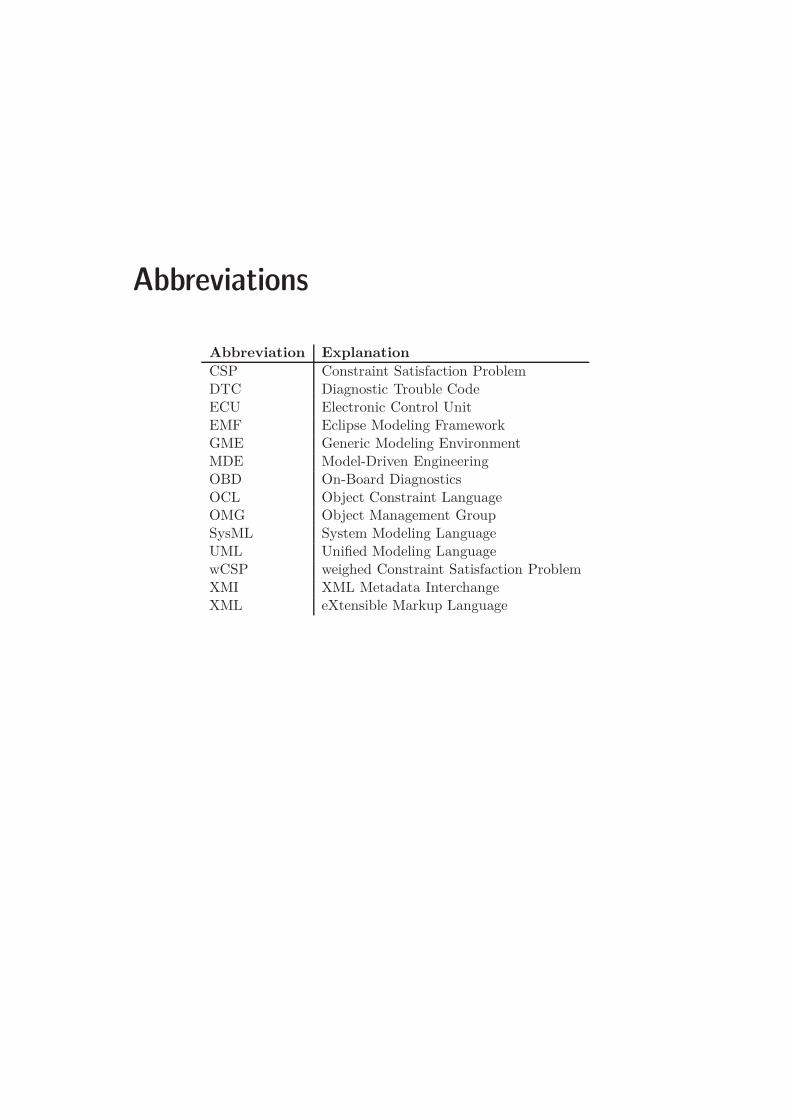
Abbreviations

Abbreviation Explanation

CSP Constraint Satisfaction ProblemDTC Diagnostic Trouble CodeECU Electronic Control UnitEMF Eclipse Modeling FrameworkGME Generic Modeling EnvironmentMDE Model-Driven EngineeringOBD On-Board DiagnosticsOCL Object Constraint LanguageOMG Object Management GroupSysML System Modeling LanguageUML Unified Modeling LanguagewCSP weighed Constraint Satisfaction ProblemXMI XML Metadata InterchangeXML eXtensible Markup Language

Chapter 1

Introduction

1.1 Background

Today, every vehicle has some on-board diagnostic system (OBD). There are basi-cally two reasons why. First of all there are legislations in this area, such as theEuropean emission standards [8]. The other reason is that a powerful diagnosticsystem dramatically can reduce the time spent at repair shop. For a commercialtransport company, reducing the time of standstill will have a substantial econom-ical benefit.

1.2 Problem definition

In the beginning of the 90’s, when the first vehicle diagnosis system came, therewas a one to one relation between tests and sensors. Nowadays there are severaltests monitoring the same sensor in different aspects. To be able to perform faultisolation in a diagnosis system, you need to know how the tests are related to thesensors or components and its different behavioral modes [4].

Today, at Scania, this kind of information is stored in a database. In this thesiswe will look at an approach where this information is described in a data modelinstead. The aim of using a modeling environment instead is to get a better overviewof the relations and get a more intuitive interface.

1.3 Objective

The objectives of this work is to:

• Evaluate different modeling environments in a perspective of the Scania re-quirements for modeling environments in the context of diagnostic informa-tion.

• Based on the evaluation, a recommendation for future works at Scania in thefield of modeling environments for diagnostic information should be made.

1

CHAPTER 1. INTRODUCTION

• Along with the master thesis worker Johan Björling develop a complete sys-tem, containing all parts from modeling a fault isolation problem until pro-viding a specific diagnosis for a system behavior. The fault isolation problemis in this approach described as a constraint satisfaction problem (CSP). Thefault isolation is done by solving this problem.

1.4 Strategy

The thesis process can be divided into the following steps:

• Introduction to diagnosis and data modeling

• Creating a meta model for diagnostic information

• Implement fault isolation structure for a retarder in one modeling environment

• Make comparison and evaluation between different modeling environments

• Write thesis report

During the project, I and my co-worker Johan had eight reference group meet-ings. Participants in the reference group were: Jonas Biteus, Mattias Nyberg, TonyLindgren, Ulf Bergman, Lars Bergström and Carl Svärd. Almost every week wehad meetings with our supervisor, Jonas Biteus.

1.5 Target group

Target group for this thesis is engineers and researchers in the domains of datamodeling, model based fault diagnosis and fault isolation and constraint satisfactionproblems. The thesis is written in a way that also students with basic knowledge ofthese areas should be able to read.

1.6 Related work

This master thesis work is one part of an ongoing venture on diagnosis at Scania.This thesis is directly related to Johan Björling’s master thesis [5] about implement-ing a weighted-CSP solver. Johan’s work is carried out at the same department asmine.

1.7 Contributions

The main contributions of this work are:

• The F-JOB framework, that covers all steps from creating a model until arunning fault isolation algorithm

2

1.8. THESIS OUTLINE

• A GME meta model for managing diagnostic information

• An implementation of fault isolation structure for a retarder using the GMEmeta model

• A comparison of Generic Modeling Environment (GME) and Topcased, basedon the Scania requirements for modeling environments

1.8 Thesis outline

Chapter 1: Introduction This chapter gives a short introduction to why diag-nosis is important in vehicles. The objectives of this thesis are presented.

Chapter 2: The F-JOB diagnosis framework This chapter presents the F-JOBdiagnosis framework, formed by this thesis together with [5]. The frameworkcovers the complete sequence from modeling the system, with respect to faultisolation, to providing a valid diagnosis at the on-board system in the vehicle.

Chapter 3: Background to model based fault diagnosis This chapter givesa background to model based fault diagnosis. This chapter gives a readerwithout a background in diagnosis a basic knowledge in this area.

Chapter 4: Background to constraint satisfaction problems This chaptergives a general background to CSP. Also weighted-CSP is described. Includesan outline for a CSP solver. This chapter is taken directly from [5].

Chapter 5: Background to meta models The layered structure of models, metamodels and meta meta models are presented. This chapter also contains smallintroductions to the UML, SysML and ECore modeling languages.

Chapter 6: Requirements for modeling environments This chapter presentsand describes the Scania requirements for modeling environments.

Chapter 7: Assessment of modeling environments In this chapter an as-sessment of the modeling environments GME and Topcased is made. Theassessment is based on the requirements described in Chapter 6.

Chapter 8: Creating a meta model for fault isolation In this chapter therequirements for a meta model for fault isolation are presented. The chaptergives also a description of a implemented meta model using GME.

Chapter 9: Implementation of fault isolation models Using the meta modelformalized in Chapter 8 to different fault isolation models are created in thischapter. The chapter also describes how the Builder object network in GMEcan be used to implement functionality for the models.

3

CHAPTER 1. INTRODUCTION

Chapter 10: Exporting model into CSP instance This chapter describes howa model in like them created in Chapter 9 can be exported into a CSP in-stance. The CSP instance file format should be readable from the CSP Solverdescribed in [5].

Chapter 11: Conclusions In this chapter conclusions and future works in thearea of this thesis are presented.

4

Chapter 2

The F-JOB diagnosis framework

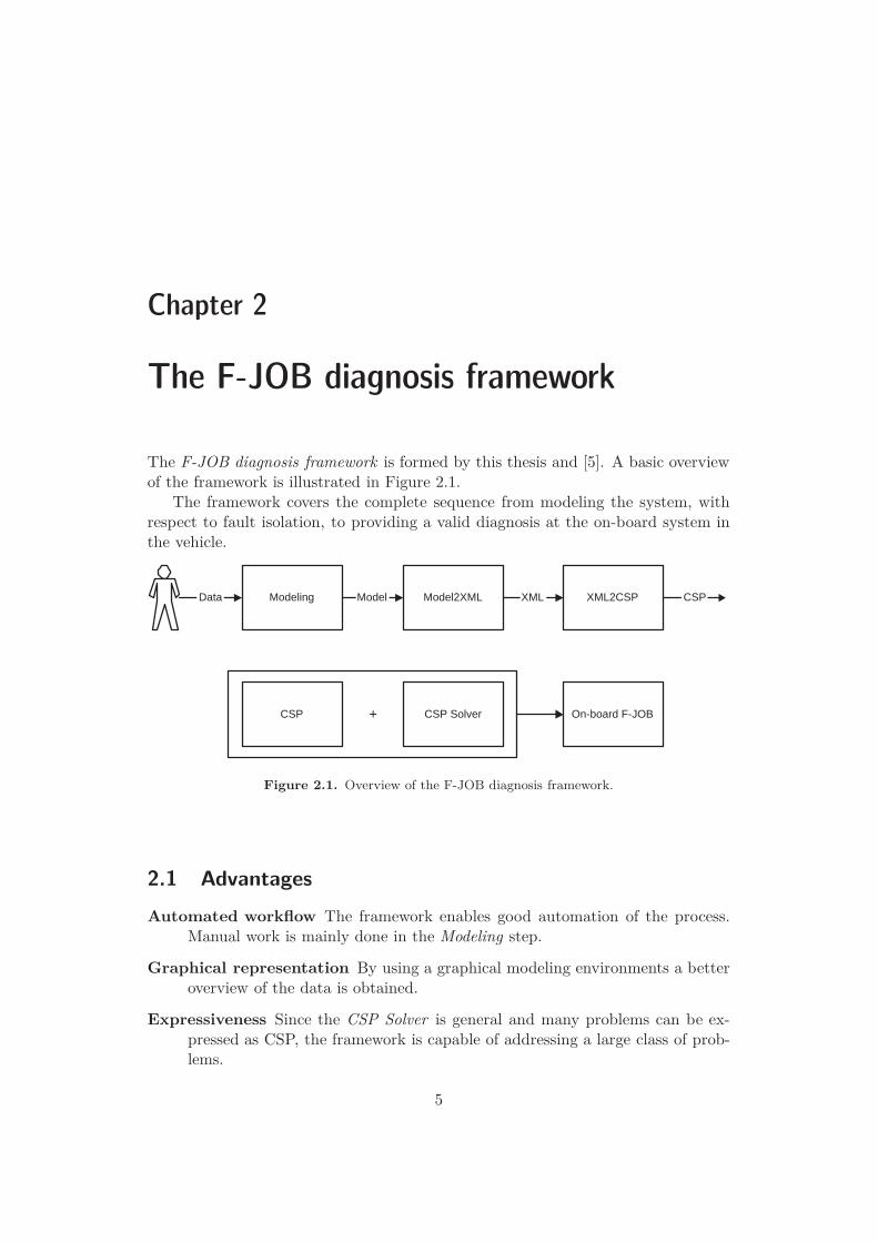
The F-JOB diagnosis framework is formed by this thesis and [5]. A basic overviewof the framework is illustrated in Figure 2.1.

The framework covers the complete sequence from modeling the system, withrespect to fault isolation, to providing a valid diagnosis at the on-board system inthe vehicle.

Modeling Data Model2XML Model XML2CSP XML CSP

On-board F-JOB CSP CSP Solver +

Figure 2.1. Overview of the F-JOB diagnosis framework.

2.1 Advantages

Automated workflow The framework enables good automation of the process.Manual work is mainly done in the Modeling step.

Graphical representation By using a graphical modeling environments a betteroverview of the data is obtained.

Expressiveness Since the CSP Solver is general and many problems can be ex-pressed as CSP, the framework is capable of addressing a large class of prob-lems.

5

CHAPTER 2. THE F-JOB DIAGNOSIS FRAMEWORK

Less manual coding The CSP that should be solved using the CSP Solver is au-tomatically generated by the XML2CSP step. The only manual coding neededis to define how the information defined by the meta model is transformed intoa CSP. Then, for every instance of the meta model, this transformation is au-tomatic.

2.2 Parts of the F-JOB diagnosis framework

Modeling In this part the information about our system is structured in a mod-eling environment. The modeling step can be extended to cover more or lessinformation depending on what the system model should be used for. In themodeling step presented here, the focus is on the structures needed to performfault isolation as described in Section 8.1. The meta model used in this stepis described in Chapter 8. An applied use of the meta model is described inChapter 9.

Model2XML Most model environments have functionality to export the modelinto an eXtensible Markup Language [9] XML-based format.

XML2CSP Transforms the XML-file, produced by the previous step Model2XML,into a predefined CSP instance format. The CSP contains information aboutthe fault isolation problem. The transformation is done by the XML2CSPapplication. This application is described in Chapter 10.

CSP The fault isolation problem described as a CSP.

CSP Solver Solves the CSP describing the fault isolation problem. When solvinga CSP all variables are assigned values from their domains in such a way thatno (or at least few) constraints are violated. This part of the framework iscarried out in [5].

On-board F-JOB By combining the CSP part and CSP Solver part we get anOn-board F-JOB. The On-board F-JOB provides fault isolation functionalityin the on-board system in the vehicle.

6

Chapter 3

Background to model based fault

diagnosis

This chapter is mainly a review of chapter 2 and 3 in [14].

3.1 Models

When dealing with model-based diagnosis system, first of all we need a model. Themodel contains information about how the system operates when there are no faultsin the system.

The model can be described using first order logic. To be able to describe themodel we use propositions, logical connectives, predicates, functions, variables, andsentences.

A proposition can either be > (TRUE) or ⊥ (FALSE). An example could be

CarColorIsGreen (3.1)

If the car is green, the proposition (3.1) is >. If the car is of some other color,the proposition (3.1) is ⊥.

Logical connectives are used to combine propositions. The most common are:¬ (not), ∧ (and), ∨ (or), → (implies), ↔ (if-and-only-if).

Propositions are possible to express as predicates. The proposition (3.1) can beexpressed as

Green(Car) (3.2)

The predicate Green(.) has arity one, since it only takes one argument. It’s alsopossible to use predicates to describe relations between objects. This is done byusing two arguments, arity two. An example could be

SameColor(Bicycle, Car) (3.3)

More flexibility is obtained by functions. Functions takes an object as argumentand returns some object. For example the color of an object can be represented by

7

CHAPTER 3. BACKGROUND TO MODEL BASED FAULT DIAGNOSIS

the function Color(.). If we combine this function with the predicate Equals(.,.),or = for short, we can write

Color(Car) = Green (3.4)

instead of Green(Car) as in 3.2.To get a more compact and flexible language, variables can be used to refer

objects. Instead of Color(Car), we can write ccar. Then we can write ccar = Greeninstead of Green(Car) as in 3.2. This is called an assignment. All possible valuesfor the variable is called it’s domain. To express the domain of the variable ccar wecan write

ccar ∈ {Green,Red,Black} (3.5)

By combining propositions, logical connectives, predicates, and variables into avalid expression we obtain a sentence. A model of a system is a set of sentencesdescribing the system.

3.2 Models for diagnosis

Models, as described in section 3.1, can be used for different purposes. In thisthesis the purpose for the model is to reason about if faults exist in the systemdescribed by the model. To achieve this, observations from the system is used, seeSection 3.2.2. A model used for diagnosis is called a diagnostic model.

3.2.1 Components and behavioral modes

To describe faults, a convention in the area of model based diagnosis is to introducethe concept of component. A component is something that could break; becomefaulty or non-faulty.

In general there could be different reasons why a component can break or becomefaulty. By this, it is common to talk about the component’s behavioral mode. Sincesome of the behavioral modes represent that the component is broken, behavioralmode sometimes are referred to as fault mode. Normally the behavioral modes fora component are no fault and one or more fault modes. A component could be inexactly one behavioral mode at the same time.

Often it is convenient to refer to all behavioral modes for all components in asystem. This is called system behavioral modes. The system behavioral mode is aconjunction of the current behavioral modes for all components in the system. Ifthe system for instance consists of two components, c1 and c2, and both componentswork fine; the system behavioral mode is OK(c1) ∧OK(c2).

3.2.2 Observations

To be able to perform the diagnosis task we need observations from the system.These observations can either be done by a human or by a automatic diagnosis

8

3.3. DIAGNOSIS DEFINITIONS

system. Observations can be seen as assigning values to variables in the model.These variables could be called observabels.

3.2.3 Example

Example 3.1: System model for a bicycle

This example is taken directly from [14].Consider first the subsystem of the bicycle consisting of the pedals, the chain,

and the back wheel. In a simplified case we can assume that in this subsystem theonly part that can brake is the chain. Therefore, the chain is our only diagnosedcomponent. Its behavioral modes are Broken and Connected. By knowledge of howa bicycle is constructed we know that if we move the pedals forward and the chainis connected, then the back wheel will also move forward. All this knowledge canformally be represented in a model as follows.

bChain ∈ Broken,Connected

rPed ∈ Backward, Standstill, Forward

rBW ∈ Backward, Standstill, Forward

bChain = Connected ∧ rPed = Forward→ rBW = Forward

Note that this model has three variables: the behavioral mode bChain, and theobservabels rPed and rBW .

If we observe that the pedals are rotating forward and the back wheel is not, wecan introduce these observational knowledge as the additional sentences

rPed = Forward

rBW = Standstill

Then there is only one possible assignment to the three variables:

bChain = Broken

rPed = Forward

rBW = Standstill

All other assignments result in a contradiction. Thus, the only diagnosis isbChain = Broken.

3.3 Diagnosis definitions

Definition 1 (Diagnosis). Given a diagnostic model M and observations Obs, adiagnosis is an assignment D of a behavioral mode to each diagnosed component

9


Fault isolation

Diagnostic test

Diagnostic test

Diagnostic test

Diagnostic test

Diagnostic test

Observations

Diagnostic statement

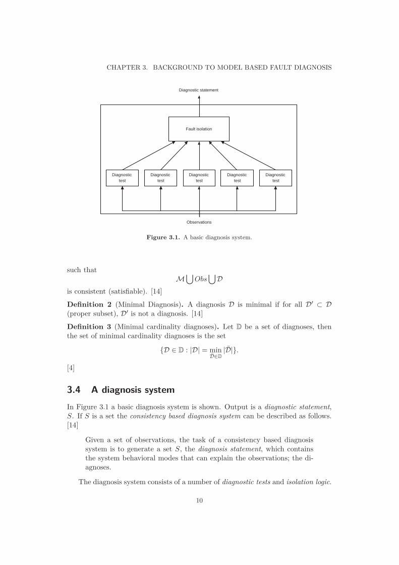
Figure 3.1. A basic diagnosis system.

such thatM⋃

Obs⋃

D

is consistent (satisfiable). [14]

Definition 2 (Minimal Diagnosis). A diagnosis D is minimal if for all D′ ⊂ D(proper subset), D′ is not a diagnosis. [14]

Definition 3 (Minimal cardinality diagnoses). Let D be a set of diagnoses, thenthe set of minimal cardinality diagnoses is the set

{D ∈ D : |D| = minD̄∈D

|D̄|}.

[4]

3.4 A diagnosis system

In Figure 3.1 a basic diagnosis system is shown. Output is a diagnostic statement,S. If S is a set the consistency based diagnosis system can be described as follows.[14]

Given a set of observations, the task of a consistency based diagnosissystem is to generate a set S, the diagnosis statement, which containsthe system behavioral modes that can explain the observations; the di-agnoses.

The diagnosis system consists of a number of diagnostic tests and isolation logic.

10

3.4. A DIAGNOSIS SYSTEM

3.4.1 Diagnostic tests

Each diagnostic test is used to determine if some specific system behavioral mode ispresent or not. All tests are binary, output is either > or ⊥. In a Scania truck thereexist two different categories of tests, electrical tests and plausibility tests. Electricaltests check for example if a given sensor value (in Volt) is inside the possible range ofvalues. Plausibility tests use more detailed models of the expected system behavioralto detect faults. How diagnostic tests are created and implemented is not discussedin this thesis.

3.4.2 Fault isolation

The fault isolation part is used to, based on all diagnostic tests in the system, formthe diagnosis statement S. There exist different approaches for the fault isolationstep in the diagnosis system. In this section we will mainly look at the column basedapproach.

In the fault isolation step it is common to prefer minimal cardinality diagnoses(see Definition 3), since faults in multiple components are less likely than singlecomponent faults.

Influence structure

In the column based approach we can look at all tests and behavioral modes ina matrix view. The matrix is called influence structure. The influence structuredescribes how the faults ideally affect the diagnostic tests. Each row, i, correspondsto a diagnostic test, Ti, and each column corresponds to a system behavioral modeFj .

Aij =

0 if Ti never reacts to any faults in fault mode FjX if Ti reacts for some operating conditions to some faults in

fault mode Fj1 if Ti always reacts to all faults in fault mode Fj

(3.6)

There is a matrix similar to the influence structure called decision structure.The decision structure describes how the diagnosis statement depends on the diag-nostic tests. When constructing this structure, also unmodeled disturbances andmeasurement noise are taken into account.

Logical representation

As seen in Equation 3.6 an influence structure can be described by logical state-ments.

11


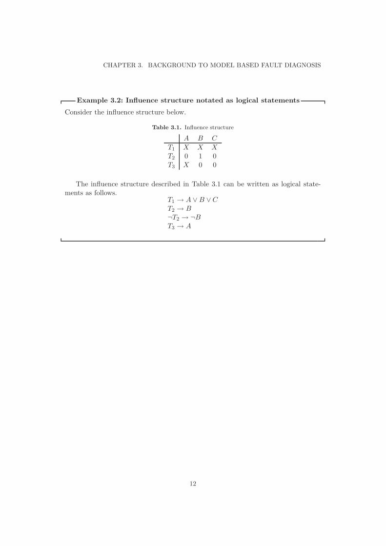
Example 3.2: Influence structure notated as logical statements

Consider the influence structure below.

Table 3.1. Influence structure

A B C

T1 X X X

T2 0 1 0T3 X 0 0

The influence structure described in Table 3.1 can be written as logical state-ments as follows.

T1 → A ∨B ∨CT2 → B¬T2 → ¬BT3 → A

12

3.4. A DIAGNOSIS SYSTEM

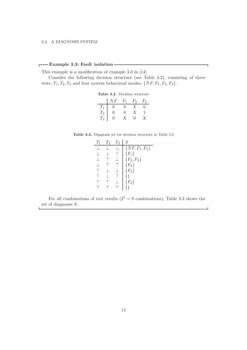
Example 3.3: Fault isolation

This example is a modification of example 3.3 in [14].Consider the following decision structure (see Table 3.2), consisting of three

tests, T1, T2, T3 and four system behavioral modes, {NF,F1, F2, F3}.

Table 3.2. Decision structure

NF F1 F2 F3

T1 0 0 X 0T2 0 0 X 1T3 0 X 0 X

Table 3.3. Diagnosis set for decision structure in Table 3.2

T1 T2 T3 S

⊥ ⊥ ⊥ {NF,F1, F2}⊥ ⊥ > {F1}⊥ > ⊥ {F2, F3}⊥ > > {F3}> ⊥ ⊥ {F2}> ⊥ > {}> > ⊥ {F2}> > > {}

For all combinations of test results (23 = 8 combinations), Table 3.3 shows theset of diagnoses S.

13

Chapter 4

Background to constraint satisfaction

problems1

4.1 Definition of CSP

A Constraint Satisfaction Problem (CSP) is a very general form of looking at aproblem, where the possible combinations of values which can exist in a solutionis constrained [1]. The framework of a CSP is simple yet very powerful whichcaptures a wide range of problems [12]. For instance, the N-queens problem, theSEND-MORE-MONEY problem and all SAT problems are CSPs [1, 2]. CSPs alsoappear in many real-life situations like scheduling, timetabling, resource allocation,etc [15, 19].

”To model a problem as a constraint satisfaction problem (CSP), wespecify a search space using a set of variables each of which can beassigned a value from some finite domain of values. To specify theassignments that solve the problem, the model includes constraints thatrestrict the set of acceptable assignments. Each constraint is over somesubset of the variables and imposes a restriction on the simultaneousvalues these variables may take.”

[2]

The definition of a CSP is very general, and contains several NP-complete prob-lems, in turn making the constraint satisfaction problem NP-complete [1].

Let V = {v1, . . . , vk} be a set of variables. A constraint, Cj on V, is a pair{RV,V} where RV is a relation on some of the variables in V. In other words, RV

is a subset of the Cartesian product of the domains of the variables in V [12, 1, 21].

1This chapter is taken directly from [5].

15

CHAPTER 4.

A Constraint Satisfaction Problem, P, consists of a triple P = {V,D,C}, whereV is a finite sequence of variables, V = {v1, . . . , vk}, each vi ∈ V has a domainDi ∈ D and C is a set of constraints [12, 1, 7, 20].

The arity of a constraint is the number of variables affected by the relation ofthe constraint [1].

An instantiation is the assignment of a value dj ∈ Di to variable vi [1, 7].A constraint, Ci ∈ Dk × . . . × Dl, is satisfiable if there exist an instantiation,

(dk, . . . , dl) ∈ D, of the variables, (vk, . . . , vl) ∈ V, participating in the constraintsuch that (dk, . . . , dl) ∈ Ci [1, 7]. From this follows that a solution is an instantiationof all vi ∈ V such that all constraints are satisfied [21, 7, 1].

A constraint is locally consistent if it is satisfiable, given some partial instanti-ation of the variables. Otherwise it is locally inconsistent [1]. A CSP is consistentif all constraints are locally consistent, and inconsistent otherwise [1].

The creation of a CSP is called modeling, and the creator of the CSP is calledthe modeler [1].

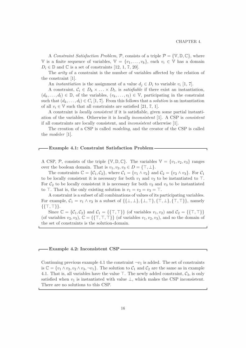
Example 4.1: Constraint Satisfaction Problem

A CSP, P, consists of the triple {V,D,C}. The variables V = {v1, v2, v3} rangesover the boolean domain. That is v1, v2, v3 ∈ D = {>,⊥}.

The constraints C = {C1, C2}, where C1 = {v1 ∧ v2} and C2 = {v2 ∧ v3}. For C1

to be locally consistent it is necessary for both v1 and v2 to be instantiated to >.For C2 to be locally consistent it is necessary for both v2 and v3 to be instantiatedto >. That is, the only existing solution is v1 = v2 = v3 = >.

A constraint is a subset of all combinations of values of its participating variables.For example, C1 = v1 ∧ v2 is a subset of {{⊥,⊥}, {⊥,>}, {>,⊥}, {>,>}}, namely{{>,>}}.

Since C = {C1, C2} and C1 = {{>,>}} (of variables v1, v2) and C2 = {{>,>}}(of variables v2, v3), C = {{>,>,>}} (of variables v1, v2, v3), and so the domain ofthe set of constraints is the solution-domain.

Example 4.2: Inconsistent CSP

Continuing previous example 4.1 the constraint ¬v1 is added. The set of constraintsis C = {v1 ∧ v2, v2 ∧ v3,¬v1}. The solution to C1 and C2 are the same as in example4.1. That is, all variables have the value >. The newly added constraint, C3, is onlysatisfied when v1 is instantiated with value ⊥, which makes the CSP inconsistent.There are no solutions to this CSP.

16

4.2. DEFINITION OF WEIGHTED CSP (WCSP)

4.2 Definition of Weighted CSP (wCSP)

A Weighted Constraint Satisfaction Problem (wCSP) is a special-case of a CSP,where weights are attached to each constraint. A Cost-Optimization Function(COF) describes what is sought after in a solution. [1]

A wCSP consists of the 4-tuple P = {V,D,C,K}, where V is a finite sequenceof variables, D contain the variables’ domains, C is a set of constraints. So V,D,C

can be viewed as a CSP. Each constraint Ci ∈ C is associated with a cost (weight)ki ∈ K. Given a partial instantiation, if Ci ∈ C is locally inconsistent, a penaltycost of ki is incurred. [1, 3]

A solution to a wCSP is an instantiation of the variables such that the cumulatedcost (weight) of all locally inconsistent constraints is minimal [1, 3].

In a wCSP, it is allowed to have locally inconsistent constraints in a solution.The difference between instantiations is the cumulated penalty cost of locally in-consistent constraints. Apart from this, a wCSP is defined in the same way as aCSP in section 4.1.

Note that according to [1], a wCSP is a special-case of a CSP. Throughoutthis thesis, the implemented solver is sometimes called CSP-solver and sometimeswCSP-solver.

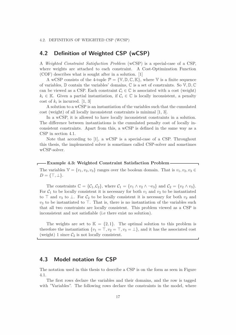
Example 4.3: Weighted Constraint Satisfaction Problem

The variables V = {v1, v2, v3} ranges over the boolean domain. That is v1, v2, v3 ∈D = {>,⊥}.

The constraints C = {C1, C2}, where C1 = {v1 ∧ v2 ∧ ¬v3} and C2 = {v2 ∧ v3}.For C1 to be locally consistent it is necessary for both v1 and v2 to be instantiatedto > and v3 to ⊥. For C2 to be locally consistent it is necessary for both v2 andv3 to be instantiated to >. That is, there is no instantiation of the variables suchthat all two constraints are locally consistent. This problem viewed as a CSP isinconsistent and not satisfiable (i.e there exist no solution).

The weights are set to K = {2, 1}. The optimal solution to this problem istherefore the instantiation {v1 = >, v2 = >, v3 = ⊥}, and it has the associated cost(weight) 1 since C2 is not locally consistent.

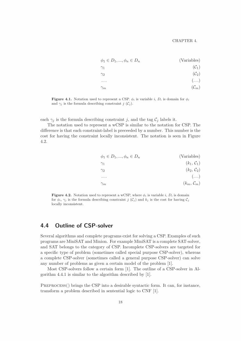
4.3 Model notation for CSP

The notation used in this thesis to describe a CSP is on the form as seen in Figure4.1.

The first rows declare the variables and their domains, and the row is taggedwith ”Variables”. The following rows declare the constraints in the model, where

17

CHAPTER 4.

φ1 ∈ D1, ..., φn ∈ Dn (Variables)

γ1 (C1)

γ2 (C2)

. . . (. . .)

γm (Cm)

Figure 4.1. Notation used to represent a CSP. φi is variable i, Di is domain for φiand γj is the formula describing constraint j (Cj).

each γj is the formula describing constraint j, and the tag Cj labels it.The notation used to represent a wCSP is similar to the notation for CSP. The

difference is that each constraint-label is preceeded by a number. This number is thecost for having the constraint locally inconsistent. The notation is seen in Figure4.2.

φ1 ∈ D1, ..., φn ∈ Dn (Variables)

γ1 (k1, C1)

γ2 (k2, C2)

. . . (. . .)

γm (km, Cm)

Figure 4.2. Notation used to represent a wCSP, where φi is variable i, Di is domainfor φi, γj is the formula describing constraint j (Cj) and kj is the cost for having Cjlocally inconsistent.

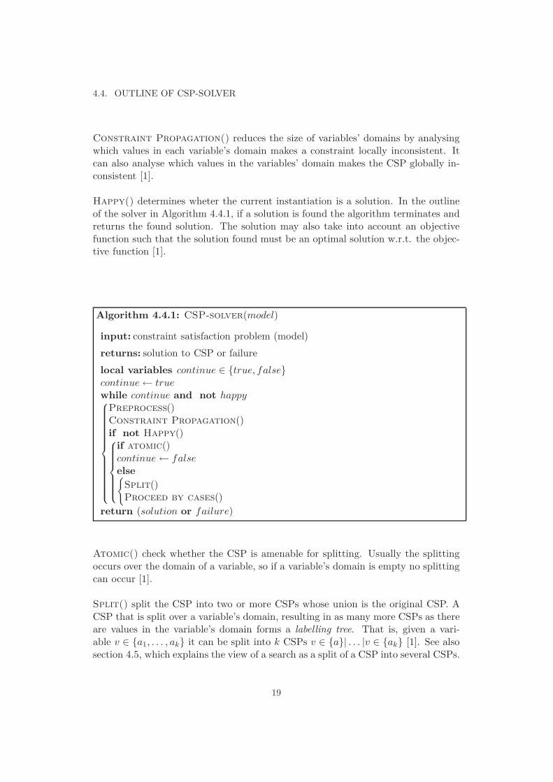
4.4 Outline of CSP-solver

Several algorithms and complete programs exist for solving a CSP. Examples of suchprograms are MiniSAT and Minion. For example MiniSAT is a complete SAT-solver,and SAT belongs to the category of CSP. Incomplete CSP-solvers are targeted fora specific type of problem (sometimes called special purpose CSP-solver), whereasa complete CSP-solver (sometimes called a general purpose CSP-solver) can solveany number of problems as given a certain model of the problem [1].

Most CSP-solvers follow a certain form [1]. The outline of a CSP-solver in Al-gorithm 4.4.1 is similar to the algorithm described by [1].

Preprocess() brings the CSP into a desirable syntactic form. It can, for instance,transform a problem described in sentential logic to CNF [1].

18

4.4. OUTLINE OF CSP-SOLVER

Constraint Propagation() reduces the size of variables’ domains by analysingwhich values in each variable’s domain makes a constraint locally inconsistent. Itcan also analyse which values in the variables’ domain makes the CSP globally in-consistent [1].

Happy() determines wheter the current instantiation is a solution. In the outlineof the solver in Algorithm 4.4.1, if a solution is found the algorithm terminates andreturns the found solution. The solution may also take into account an objectivefunction such that the solution found must be an optimal solution w.r.t. the objec-tive function [1].

Algorithm 4.4.1: CSP-solver(model)

input: constraint satisfaction problem (model)

returns: solution to CSP or failure

local variables continue ∈ {true, false}continue← truewhile continue and not happy

Preprocess()Constraint Propagation()if not Happy()

if atomic()continue← falseelse{

Split()Proceed by cases()

return (solution or failure)

Atomic() check whether the CSP is amenable for splitting. Usually the splittingoccurs over the domain of a variable, so if a variable’s domain is empty no splittingcan occur [1].

Split() split the CSP into two or more CSPs whose union is the original CSP. ACSP that is split over a variable’s domain, resulting in as many more CSPs as thereare values in the variable’s domain forms a labelling tree. That is, given a vari-able v ∈ {a1, . . . , ak} it can be split into k CSPs v ∈ {a}| . . . |v ∈ {ak} [1]. See alsosection 4.5, which explains the view of a search as a split of a CSP into several CSPs.

19

CHAPTER 4.

Proceed By Cases() is the search function in which each CSP (from the Split()function) is considered in a certain order. The order depends on the adopted search-technique. The backtracking search, for instance, traverses the tree generated in aform of chronological order where it starts with each variable’s first value [3, 1].

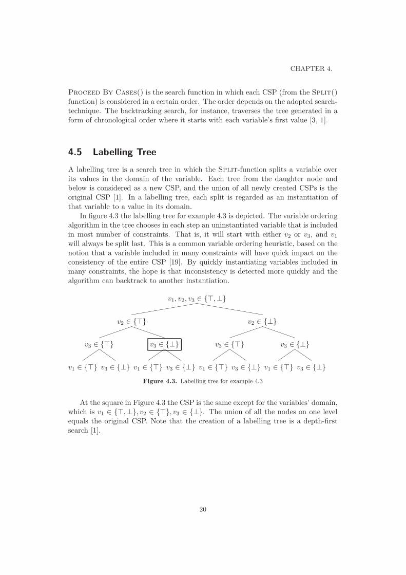
4.5 Labelling Tree

A labelling tree is a search tree in which the Split-function splits a variable overits values in the domain of the variable. Each tree from the daughter node andbelow is considered as a new CSP, and the union of all newly created CSPs is theoriginal CSP [1]. In a labelling tree, each split is regarded as an instantiation ofthat variable to a value in its domain.

In figure 4.3 the labelling tree for example 4.3 is depicted. The variable orderingalgorithm in the tree chooses in each step an uninstantiated variable that is includedin most number of constraints. That is, it will start with either v2 or v3, and v1will always be split last. This is a common variable ordering heuristic, based on thenotion that a variable included in many constraints will have quick impact on theconsistency of the entire CSP [19]. By quickly instantiating variables included inmany constraints, the hope is that inconsistency is detected more quickly and thealgorithm can backtrack to another instantiation.

v1, v2, v3 ∈ {>,⊥}

v2 ∈ {>} v2 ∈ {⊥}

v3 ∈ {>} v3 ∈ {⊥} v3 ∈ {>} v3 ∈ {⊥}

v1 ∈ {>} v3 ∈ {⊥} v1 ∈ {>} v3 ∈ {⊥} v1 ∈ {>} v3 ∈ {⊥} v1 ∈ {>} v3 ∈ {⊥}

Figure 4.3. Labelling tree for example 4.3

At the square in Figure 4.3 the CSP is the same except for the variables’ domain,which is v1 ∈ {>,⊥}, v2 ∈ {>}, v3 ∈ {⊥}. The union of all the nodes on one levelequals the original CSP. Note that the creation of a labelling tree is a depth-firstsearch [1].

20

Chapter 5

Background to meta models

5.1 Introduction

A model is an abstract and simplified description of reality, designed to mirror somespecific properties of the real world and ignore some others. In this sense, modelsare always simplifications. A meta model is a model that describes models. In thisway, meta models constrain what models can contain, and make sure that differentinstantiated models are standardized and comparable. A meta meta model doesthe same for a meta model. In principle, we can go on and add new meta levelsindefinitely. In practice, the use of four abstraction levels is widely adopted.

5.2 Model-driven engineering

Model-driven engineering (MDE) is a software development methodology that fo-cuses on models of the software to be developed. The basic idea is that there areseveral different useful abstraction levels of such models, that can be used for differ-ent purposes. For example, the same program can be modeled as a platform specificmodel or more abstractly as a platform independent model. Furthermore, the no-tion of transformation is central: vertical transformations between the abstractionlevels correspond to implementations, whereas horizontal transformations remainon the same level of abstraction [17].

The long term goal of MDE is to further simplify software development in thesame way as it has already been simplified by high-level programming languages(e.g. C++) as compared to low-level languages (e.g. Assembler). While it is indeedalready possible to generate executable code from UML diagrams, there are stillnumerous issues to be resolved before the MDE vision is fulfilled [16].

Since the different abstraction levels play a crucial role in MDE, it is vital tohave precise definitions of the different abstraction levels. A prominent initiativein this area is the Object Management Group (OMG) set of standards known asModel Driven Architecture.

21

CHAPTER 5. BACKGROUND TO META MODELS

M3 Meta meta model

M2 Meta model

M1 Model

M0 User model

«uses»

«uses»

«uses»

«uses»

Figure 5.1. The four layer structure of MOF.

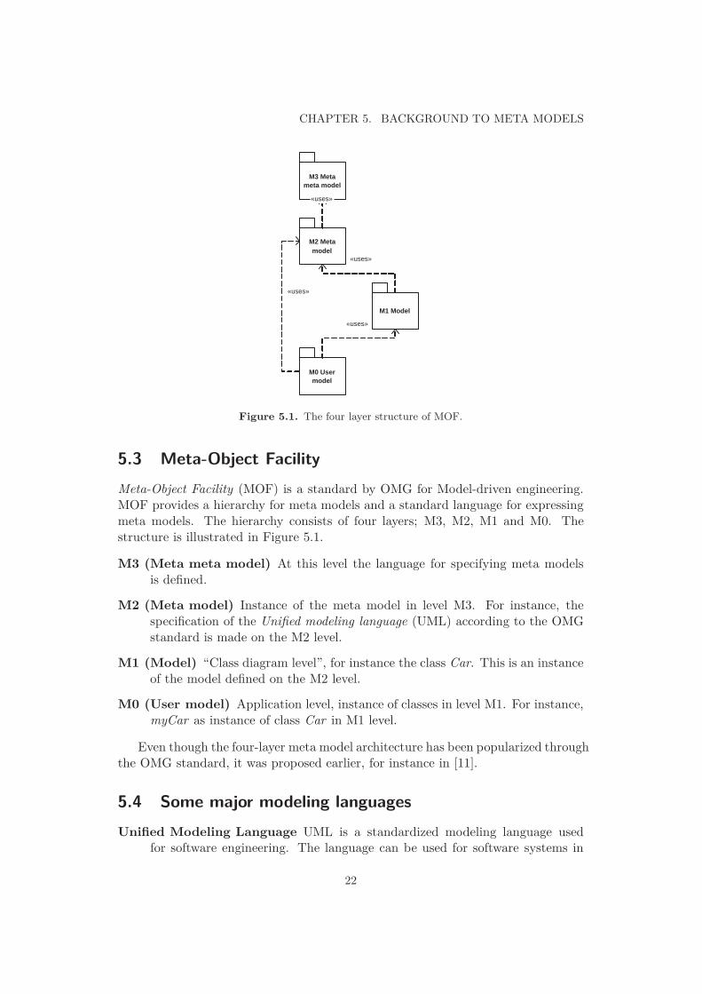
5.3 Meta-Object Facility

Meta-Object Facility (MOF) is a standard by OMG for Model-driven engineering.MOF provides a hierarchy for meta models and a standard language for expressingmeta models. The hierarchy consists of four layers; M3, M2, M1 and M0. Thestructure is illustrated in Figure 5.1.

M3 (Meta meta model) At this level the language for specifying meta modelsis defined.

M2 (Meta model) Instance of the meta model in level M3. For instance, thespecification of the Unified modeling language (UML) according to the OMGstandard is made on the M2 level.

M1 (Model) “Class diagram level”, for instance the class Car. This is an instanceof the model defined on the M2 level.

M0 (User model) Application level, instance of classes in level M1. For instance,myCar as instance of class Car in M1 level.

Even though the four-layer meta model architecture has been popularized throughthe OMG standard, it was proposed earlier, for instance in [11].

5.4 Some major modeling languages

Unified Modeling Language UML is a standardized modeling language usedfor software engineering. The language can be used for software systems in

22

5.4. SOME MAJOR MODELING LANGUAGES

UML UML for SysML

SysML

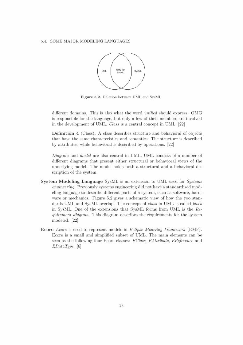
Figure 5.2. Relation between UML and SysML.

different domains. This is also what the word unified should express. OMGis responsible for the language, but only a few of their members are involvedin the development of UML. Class is a central concept in UML. [22]

Definition 4 (Class). A class describes structure and behavioral of objectsthat have the same characteristics and semantics. The structure is describedby attributes, while behavioral is described by operations. [22]

Diagram and model are also central in UML. UML consists of a number ofdifferent diagrams that present either structural or behavioral views of theunderlying model. The model holds both a structural and a behavioral de-scription of the system.

System Modeling Language SysML is an extension to UML used for Systemsengineering. Previously systems engineering did not have a standardized mod-eling language to describe different parts of a system, such as software, hard-ware or mechanics. Figure 5.2 gives a schematic view of how the two stan-dards UML and SysML overlap. The concept of class in UML is called blockin SysML. One of the extensions that SysML forms from UML is the Re-quirement diagram. This diagram describes the requirements for the systemmodeled. [22]

Ecore Ecore is used to represent models in Eclipse Modeling Framework (EMF).Ecore is a small and simplified subset of UML. The main elements can beseen as the following four Ecore classes: EClass, EAttribute, EReference andEDataType. [6]

23

Chapter 6

Requirements for modeling

environments

6.1 Introduction

This section describes the requirements for modeling environments. The require-ments listed in Section 6.2.1 and Section 6.2.2 are based on discussions in the groupfor future diagnosis at Scania.

6.2 Requirements

Requirements can be divided into two sub-categories, functional requirements andnon-functional requirements [17].

Sommerville also mentions a third category, domain requirements. In this case,domain requirements refer to our requirements for the meta model we are creat-ing using the modeling environment. The domain requirements are described inSection 8.1.

6.2.1 Functional requirements

Functional requirements specify what functionality the system should provide. Afunctional requirement can also specify how the system should behave to particularinput or in a particular situation [17].

Below is a list containing all functional requirements that will be discussed inthe evaluation in Chapter 7.

Requirement 6.1 (Should be able to store probabilities). In some applicationsconnected to a model with diagnostic information there is a need to know theprobability that a given component is broken or not. By this, there is a need to beable to store probabilities in the model environment.

25

CHAPTER 6. REQUIREMENTS FOR MODELING ENVIRONMENTS

Requirement 6.2 (Should be able to represent time or sequences). To be able toreason about time, we need some kind of support for representing time or sequencesin the models.

Requirement 6.3 (Multi-user environment). Since there are many employees atScania working with diagnosis, the modeling environment must provide support forsome multi-user environment.

Requirement 6.4 (Support for revision control). There must be support for revi-sion control, either included in the modeling environment or by using an externalsystem.

6.2.2 Non-functional requirements

Non-functional requirements are constraints on the services or functions provided bythe system. This category of requirements includes constraints on the developmentprocess and standards.

The non-functional requirements could be categorized into three main categories;product requirements, oranisational requirements and external requirements [17].

Below is a list containing all non-functional requirements that will be discussedin the evaluation in Chapter 7.

Requirement 6.5 (Supported standards). In general it is good to have supportfor standardizations in the domain area of the software. In this case the standardSysML is one example. Also the standard for meta model interchange, XMI (XMI -XML Metadata Interchange) is desirable.

Requirement 6.6 (Existing external support, still being developed). If a modelingenvironment should be used at Scania, there will be a need for support. Is theresupport available from the manufacturer, or do Scania have to supply support them-selves? If the environment still is being developed, it is easier to keep the softwareupdated and compatible with different platforms and software.

Requirement 6.7 (License type). What license is the modeling environment dis-tributed under? Software free of charge is preferable. Is the source code available?

Requirement 6.8 (Well-known by engineers). Is the concept or workflow for themodeling environment already known by engineers? If so, the phase for startingusing the modeling environment can be reduced.

26

Chapter 7

Assessment of modeling environments

7.1 Introduction

In Chapter 6 a number of requirements for a modeling environment were presented.In this chapter we will look at how well two different modeling environments meetthese requirements.

7.2 Tools used for modeling

7.2.1 GME

GME is a research project at Vanderbilt university. In this comparison the GenericModeling Environment version 7.6.29 (released July 2007) is used. Project home-page is http://www.isis.vanderbilt.edu/projects/gme/.

The Generic Modeling Environment (GME) is intended to support the easycreation of domain-specific modeling and program synthesis environments. A mod-eling environment for graphical creating entity-relationship diagrams is provided.For ease of use, the same environment is capable of metamodeling and modeling.[13]

7.2.2 Topcased

In this comparison the Topcased version 2.5.0 (released May 2009) is used. Projecthomepage is http://www.topcased.org.

The Topcased project aims at developing an open source critical aeronauticsystems design environment for critical applications and systems development. Itprovides a graphical interface for metamodeling and support for a number of mod-eling languages, such as UML, SysML and Ecore. [10]

27

CHAPTER 7. ASSESSMENT OF MODELING ENVIRONMENTS

7.3 Assessments

For each of the requirements, an assessment is assigned to each of the two modelingenvironments. The possible assessments for a requirement are the following three:

Not acceptable (0). Means that the requirement not is met by the software, oris met in a way that not is preferable.

Acceptable (1). Means that the requirement is met by the software in an accept-able way.

Good (2). Means that the requirement is met by the software in a better way.

During this thesis project GME has been used as one of the main tools, so inthis comparison the assessments of GME have a more solid basis than the assess-ments of Topcased. In the Topcased case the assessments are mainly based ondocumentation.

7.4 Functional requirements

7.4.1 Requirement 6.1: Should be able to store probabilities

GME Acceptable (1). There is no direct support for this. However, it is possible toassign an attribute (data field) containing a probability to an atom or modelin the MetaGME paradigm. This kind of method for probabilities does notprovide any semantics for the probability, just a way to store the information.

Topcased Good (2). SysML includes support for probabilities. Since Topcasedimplements the SysML standard, this should be possible in Topcased.

7.4.2 Requirement 6.2: Should be able to represent time or sequences

GME Acceptable (1). By implementing a meta model supporting some represen-tation of a sequence, by for example using the connection in the MetaGMEparadigm, a basic time or sequence functionality is implemented. Also here,no semantics are provided.

Topcased Good (2). SysML includes support for state diagrams. Since Topcasedimplements the SysML standard, this should be possible in Topcased.

7.4.3 Requirement 6.3: Multi-user environment

GME Acceptable (1). GME provides basic multi-user functionality. See also Re-quirement 6.4.

Topcased Good (2). Topcased provides good multi-user functionality. See alsoRequirement 6.4.

28

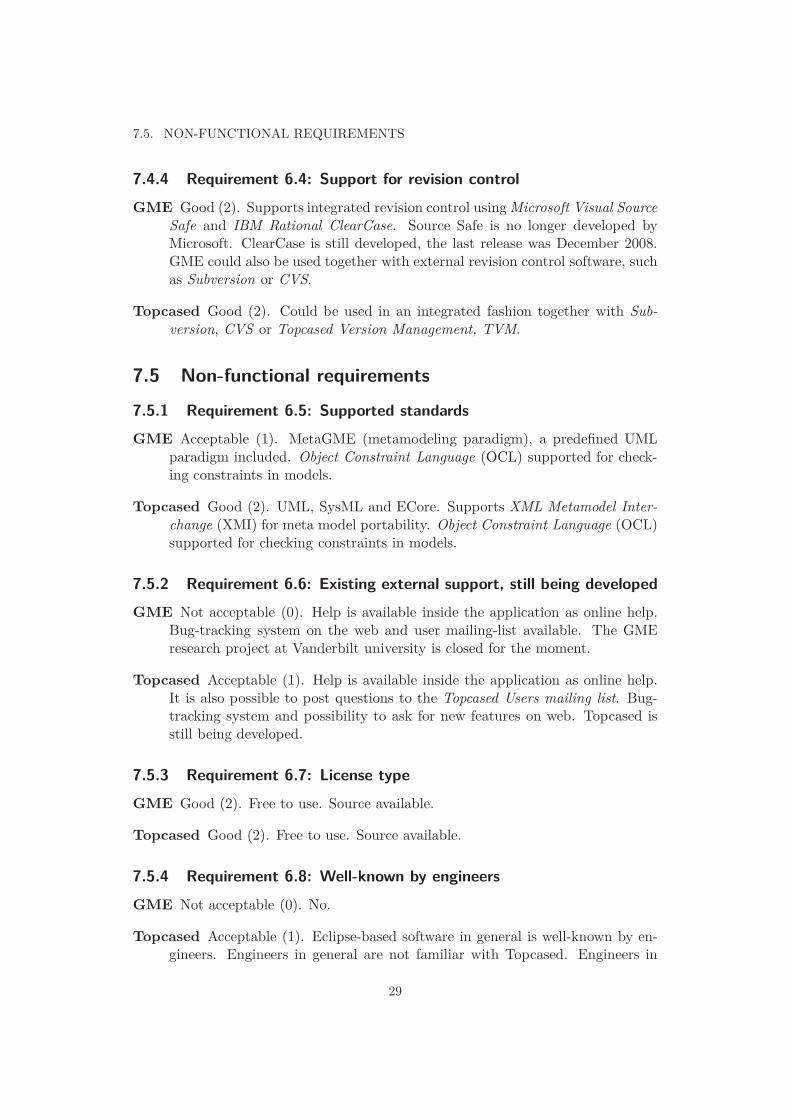
7.5. NON-FUNCTIONAL REQUIREMENTS

7.4.4 Requirement 6.4: Support for revision control

GME Good (2). Supports integrated revision control using Microsoft Visual SourceSafe and IBM Rational ClearCase. Source Safe is no longer developed byMicrosoft. ClearCase is still developed, the last release was December 2008.GME could also be used together with external revision control software, suchas Subversion or CVS.

Topcased Good (2). Could be used in an integrated fashion together with Sub-version, CVS or Topcased Version Management, TVM.

7.5 Non-functional requirements

7.5.1 Requirement 6.5: Supported standards

GME Acceptable (1). MetaGME (metamodeling paradigm), a predefined UMLparadigm included. Object Constraint Language (OCL) supported for check-ing constraints in models.

Topcased Good (2). UML, SysML and ECore. Supports XML Metamodel Inter-change (XMI) for meta model portability. Object Constraint Language (OCL)supported for checking constraints in models.

7.5.2 Requirement 6.6: Existing external support, still being developed

GME Not acceptable (0). Help is available inside the application as online help.Bug-tracking system on the web and user mailing-list available. The GMEresearch project at Vanderbilt university is closed for the moment.

Topcased Acceptable (1). Help is available inside the application as online help.It is also possible to post questions to the Topcased Users mailing list. Bug-tracking system and possibility to ask for new features on web. Topcased isstill being developed.

7.5.3 Requirement 6.7: License type

GME Good (2). Free to use. Source available.

Topcased Good (2). Free to use. Source available.

7.5.4 Requirement 6.8: Well-known by engineers

GME Not acceptable (0). No.

Topcased Acceptable (1). Eclipse-based software in general is well-known by en-gineers. Engineers in general are not familiar with Topcased. Engineers in

29

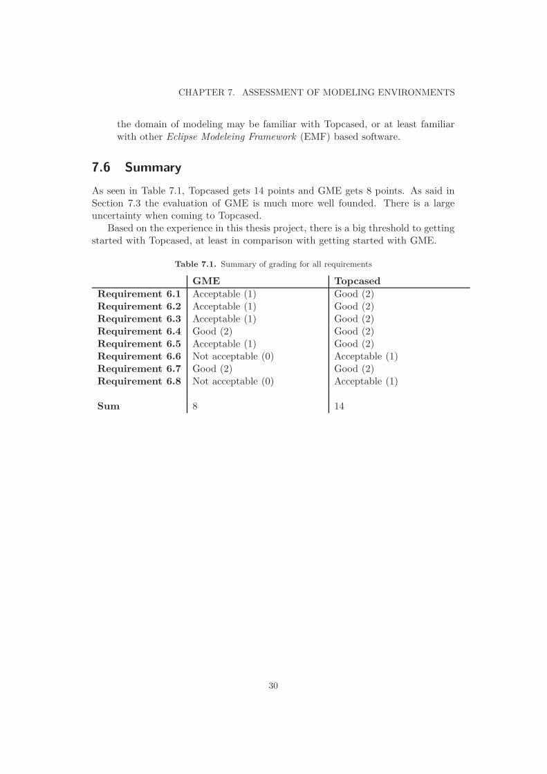
CHAPTER 7. ASSESSMENT OF MODELING ENVIRONMENTS

the domain of modeling may be familiar with Topcased, or at least familiarwith other Eclipse Modeleing Framework (EMF) based software.

7.6 Summary

As seen in Table 7.1, Topcased gets 14 points and GME gets 8 points. As said inSection 7.3 the evaluation of GME is much more well founded. There is a largeuncertainty when coming to Topcased.

Based on the experience in this thesis project, there is a big threshold to gettingstarted with Topcased, at least in comparison with getting started with GME.

Table 7.1. Summary of grading for all requirements

GME Topcased

Requirement 6.1 Acceptable (1) Good (2)Requirement 6.2 Acceptable (1) Good (2)Requirement 6.3 Acceptable (1) Good (2)Requirement 6.4 Good (2) Good (2)Requirement 6.5 Acceptable (1) Good (2)Requirement 6.6 Not acceptable (0) Acceptable (1)Requirement 6.7 Good (2) Good (2)Requirement 6.8 Not acceptable (0) Acceptable (1)

Sum 8 14

30

Chapter 8

Creating a meta model for fault

isolation

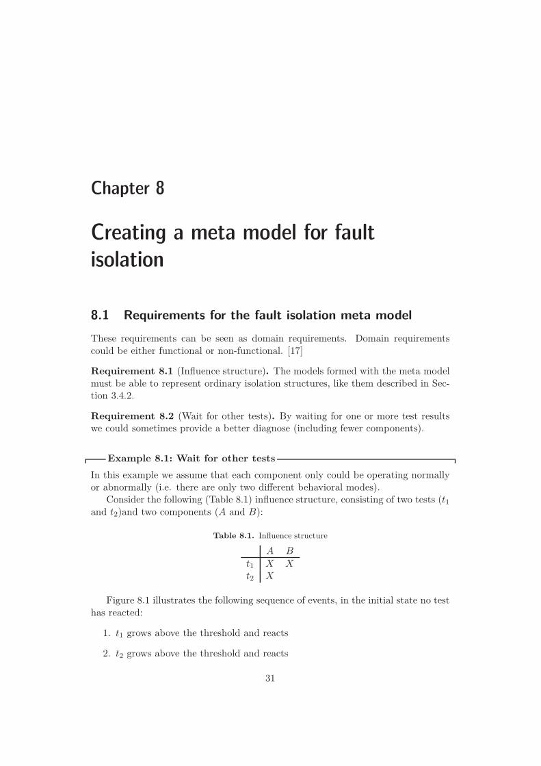
8.1 Requirements for the fault isolation meta model

These requirements can be seen as domain requirements. Domain requirementscould be either functional or non-functional. [17]

Requirement 8.1 (Influence structure). The models formed with the meta modelmust be able to represent ordinary isolation structures, like them described in Sec-tion 3.4.2.

Requirement 8.2 (Wait for other tests). By waiting for one or more test resultswe could sometimes provide a better diagnose (including fewer components).

Example 8.1: Wait for other tests

In this example we assume that each component only could be operating normallyor abnormally (i.e. there are only two different behavioral modes).

Consider the following (Table 8.1) influence structure, consisting of two tests (t1and t2)and two components (A and B):

Table 8.1. Influence structure

A B

t1 X X

t2 X

Figure 8.1 illustrates the following sequence of events, in the initial state no testhas reacted:

1. t1 grows above the threshold and reacts

2. t2 grows above the threshold and reacts

31

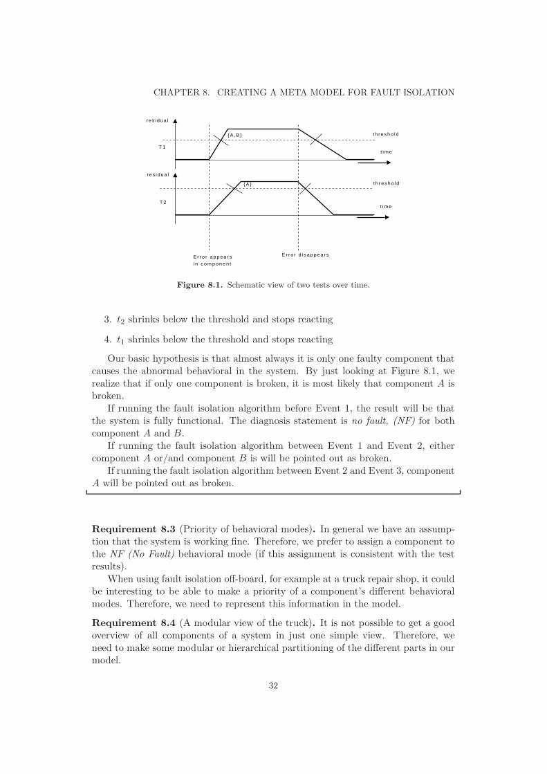
CHAPTER 8. CREATING A META MODEL FOR FAULT ISOLATION

T 1

T 2

E r r o r a p p e a r si n c o m p o n e n t

{ A , B }

{ A }

E r r o r d i s a p p e a r s

t i m e

t i m e

r e s i d u a l

r e s i d u a l

t h r e s h o l d

t h r e s h o l d

Figure 8.1. Schematic view of two tests over time.

3. t2 shrinks below the threshold and stops reacting

4. t1 shrinks below the threshold and stops reacting

Our basic hypothesis is that almost always it is only one faulty component thatcauses the abnormal behavioral in the system. By just looking at Figure 8.1, werealize that if only one component is broken, it is most likely that component A isbroken.

If running the fault isolation algorithm before Event 1, the result will be thatthe system is fully functional. The diagnosis statement is no fault, (NF) for bothcomponent A and B.

If running the fault isolation algorithm between Event 1 and Event 2, eithercomponent A or/and component B is will be pointed out as broken.

If running the fault isolation algorithm between Event 2 and Event 3, componentA will be pointed out as broken.

Requirement 8.3 (Priority of behavioral modes). In general we have an assump-tion that the system is working fine. Therefore, we prefer to assign a component tothe NF (No Fault) behavioral mode (if this assignment is consistent with the testresults).

When using fault isolation off-board, for example at a truck repair shop, it couldbe interesting to be able to make a priority of a component’s different behavioralmodes. Therefore, we need to represent this information in the model.

Requirement 8.4 (A modular view of the truck). It is not possible to get a goodoverview of all components of a system in just one simple view. Therefore, weneed to make some modular or hierarchical partitioning of the different parts in ourmodel.

32

8.2. META MODEL FORMALIZED IN GME

8.2 Meta model formalized in GME

In this thesis the meta model for fault isolation is implemented using GME. Moreinformation about GME can be found in Section 7.2.1.

8.2.1 MetaGME

MetaGME is the paradigm in GME used for meta models. [18]Available parts in MetaGME are: (Descriptions in the list below are taken, with

smaller modifications or shortening, directly from [18]).

Atom Atoms (or atomic parts) are simple modeling objects that do not have inter-nal structure (i.e. they do not contain other objects), although they can haveattributes. Atoms can be used to represent entities, which are indivisible, andexist in the context of their parent model.

Model By model we mean an abstract object that represents something in theworld. What a model represents depends on what domain we are working in.A model typically has parts - other objects contained within the model. Partscome in these varieties: atoms, other models, references, sets and connections.

Reference References are parts that are similar in concept to pointers found invarious programming languages. When complex models are created (contain-ing many, different kinds of atomic and hierarchical parts), it is sometimesnecessary for one model to directly access parts contained in another.

Reference parts are objects that refer to (i.e. point to) other modeling objects.Thus, a reference part can point to a model, an atomic part of a model, a modelembedded in another model, or even another reference part or a set.

Connection Merely having parts in a model is not sufficient for creating mean-ingful models - there are relationships among those parts that need to beexpressed. The GME uses many different methods for expressing these rela-tionships, the simplest one being the connection. A connection is a line thatconnects two parts of a model. The parts act as ports for the connection.Atoms, models, sets and references can act as ports.

The actual semantics of a connection is determined by the modeling paradigm.

Set Models containing objects and connections show a static system. In somecases, however, it is necessary to have a model of a dynamic system thathas an architecture that changes over time. From the visual standpoint thismeans that, depending on what “state” the system is in, we should see differentpictures. These “states” are not predefined by the modeling paradigm (in thatcase they would be aspects), but rather by the modeler. The different picturesshould show the same model, containing the same kinds of parts, but some ofthe parts should be “present” while others should be “missing” in a certain

33

CHAPTER 8. CREATING A META MODEL FOR FAULT ISOLATION

“states”. In other words, the modeler should be able to construct sets andsubsets of particular objects (even connections).

Parts may belong to a single set, to more than one set, or to no set at all.

Attribute Models, atoms, references, sets and connections can all have attributes.An attribute is a property of an object that is best expressed textually. (Notethat we use the word “text” for anything that is shown as text, includingnumbers, and a choice from a finite set of symbolic or numeric constants.)

The modeling paradigm defines what attributes are present for what objects,the ranges of the attribute values, etc.

Aspect Large models and/or complex modeling paradigms can lead to situationswhere, even within a given level of design hierarchy, there may be too manyparts displayed at once. To alleviate this problem, models can be partitionedinto aspects.

An aspect is defined by the kinds of parts that are visible in that aspect. Notethat aspects are related to groups of parts. The existence or visibility of apart within a particular aspect is determined by the modeling paradigm. Agiven part may also be visible in more than one aspect. When a model isviewed, it is always viewed from one particular aspect at a time.

8.2.2 Creating model using MetaGME

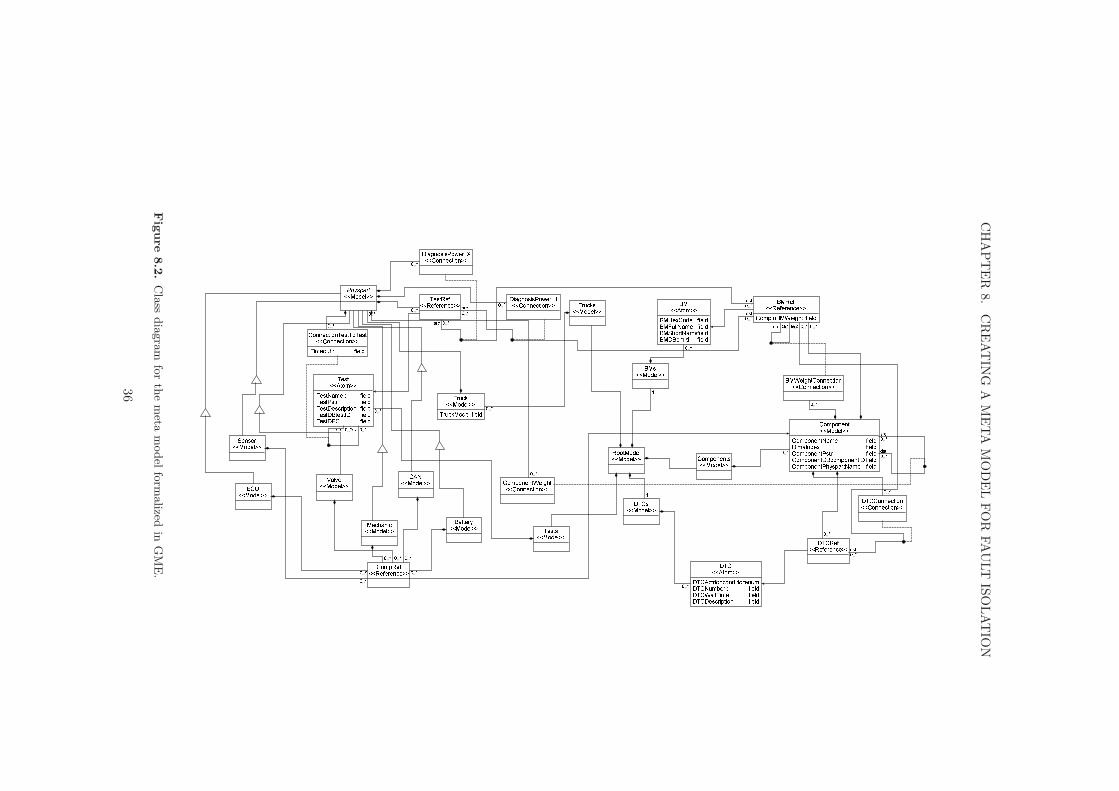
A complete class diagram for the meta model formed using the MetaGME paradigmcan be found in Figure 8.2.

The meta model consists of the following parts:

RootModel (Model) The root model holds all other models.

Trucks (Model) Model that holds the different Truck instances. Needed to meetRequirement 8.4.

Truck (Model) Represent a single truck configuration. Needed to meet Require-ment 8.4.

Physpart (Model) Used to group components into their physical parts. Neededto meet Requirement 8.4.

Test (Atom) Represents a diagnostic test. Needed to meet Requirement 8.1.

BM (Atom) Represents a behavioral mode. Needed to meet Requirement 8.1.

DTC (Atom) Represents DTC. Each DTC have a timeout in which the DTCmust be set, if the fault represented by the DTC is detected. Needed to meetRequirement 8.2.

34

8.2. META MODEL FORMALIZED IN GME

DiagnosisPower_1 (Connection) Represents 1 in an influence structure. Neededto meet Requirement 8.1.

DiagnosisPower_X (Connection) Represents X in an influence structure. Neededto meet Requirement 8.1.

BMWeightConnection (Connection) Used as binary relation between behav-ioral mode references in a component to specify if one behavioral mode ispreferable before one other. Needed to meet Requirement 8.3.

TestRef (Reference) By using references in each instance of a truck, we get lessdata redundancy. Needed to meet Requirement 8.4.

ComponentRef (Reference) By using references in each instance of a truck, weget less data redundancy. Needed to meet Requirement 8.4.

BMRef (Reference) By using references in each instance of a component, we getless data redundancy. Needed to meet Requirement 8.4.

DTCRef (Reference) By using references in each instance of a component, weget less data redundancy. Needed to meet Requirement 8.4.

Aspect1 (Aspect) All meta model must have at least one aspect, since the aspectdefines which parts of the model that are visible.

35

CH

AP

TE

R8.

CR

EA

TIN

GA

ME

TA

MO

DE

LF

OR

FA

ULT

ISO

LA

TIO

N

��

� � ��

�� ! � �� ! � ��

! � �� ! " � # �� ! " � #� � � � � � � ! " � # � � � � ��

��

� � � � ��

� � � � � � � � $� % � & '� � ��

! � � � ��

�� ! � �� ! � ! � �� ! � � �� " ��

! � �� ! �� ! �� " � ! � � " � ( � � � � � � � ! � �� ! � � �� ! � � � � ��

� � � � � � � � $� % � & )� � �� ! � �� ! � �� ! � �� $ �� ! � �� ! � �� ! � ��

*+, -./ 0 1� � � � � � � � �� 2 �3 �� 4 " � � � � � �� ( � � ��

� � � � � 5� � � � � � �

�� 3 � � � � � �� $ �� $ � 5 ��

67 7 89: ; 67 7 8:<= 67 7 8

67 7 867 7 8

67 7 867 7 8

9: ;67 7 867 7 8

67 7 8 67 7 89: ; 67 7 8

67 7 8 9: ;67 7 8

67 7 8 9: ;67 7 8 :< = 67 7 867 7 867 7 8

67 7 8:< = 67 7 8

>67 7 8

67 7 8

67 7 8

> >>

:<= 67 7 8

:< = 67 7 89: ;67 7 867 7 8

67 7 8

>67 7 8

67 7 867 7 8

:< = 67 7 8

Fig

ure

8.2

.C

lass

dia

gra

mfo

rth

em

etam

od

elfo

rmalized

inG

ME

.

36

Chapter 9

Implementation of fault isolation models

9.1 Introduction

The meta model has been tested using two different approaches.

1. Implementing a small fault isolation model by manually entering the modelin GME. This approach is described in Section 9.2.

2. Implementing a bigger fault isolation model by automatic import of data fromdatabase to GME. This approach is described in Section 9.3.

9.2 A small fault isolation model

The model consists of 11 tests and 7 components. Each component has at leastone faulty behavioral mode. Some of the components have more than one faultybehavioral mode. The influence structure for the test instance is found in Table 9.1.

Table 9.1. Influence structure for a small fault isolation model

c1 c2 c3 c4 c5 c6 c7f1 UF f1 UF f1 UF f1 f2 UF UF UF UF

t1 X

t2 X

t3 X X X X

t4 X X X X

t5 X X X X

t6 X X X

t7 1 X

t8 1t9 X X X

t10 1 X

t11 1

37

CHAPTER 9. IMPLEMENTATION OF FAULT ISOLATION MODELS

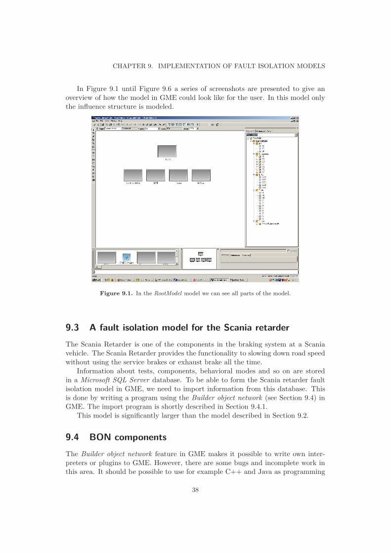
In Figure 9.1 until Figure 9.6 a series of screenshots are presented to give anoverview of how the model in GME could look like for the user. In this model onlythe influence structure is modeled.

Figure 9.1. In the RootModel model we can see all parts of the model.

9.3 A fault isolation model for the Scania retarder

The Scania Retarder is one of the components in the braking system at a Scaniavehicle. The Scania Retarder provides the functionality to slowing down road speedwithout using the service brakes or exhaust brake all the time.

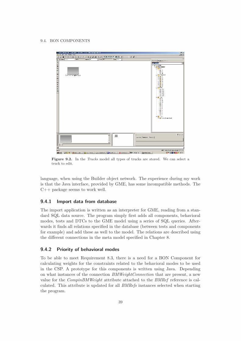
Information about tests, components, behavioral modes and so on are storedin a Microsoft SQL Server database. To be able to form the Scania retarder faultisolation model in GME, we need to import information from this database. Thisis done by writing a program using the Builder object network (see Section 9.4) inGME. The import program is shortly described in Section 9.4.1.

This model is significantly larger than the model described in Section 9.2.

9.4 BON components

The Builder object network feature in GME makes it possible to write own inter-preters or plugins to GME. However, there are some bugs and incomplete work inthis area. It should be possible to use for example C++ and Java as programming

38

9.4. BON COMPONENTS

Figure 9.2. In the Trucks model all types of trucks are stored. We can select atruck to edit.

language, when using the Builder object network. The experience during my workis that the Java interface, provided by GME, has some incompatible methods. TheC++ package seems to work well.

9.4.1 Import data from database

The import application is written as an interpreter for GME, reading from a stan-dard SQL data source. The program simply first adds all components, behavioralmodes, tests and DTCs to the GME model using a series of SQL queries. After-wards it finds all relations specified in the database (between tests and componentsfor example) and add these as well to the model. The relations are described usingthe different connections in the meta model specified in Chapter 8.

9.4.2 Priority of behavioral modes

To be able to meet Requirement 8.3, there is a need for a BON Component forcalculating weights for the constraints related to the behavioral modes to be usedin the CSP. A prototype for this components is written using Java. Dependingon what instances of the connection BMWeightConnection that are present, a newvalue for the CompinBMWeight attribute attached to the BMRef reference is cal-culated. This attribute is updated for all BMRefs instances selected when startingthe program.

39


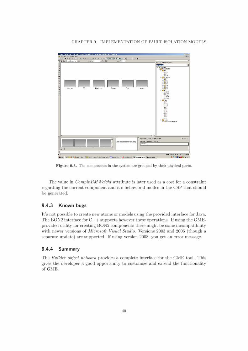
Figure 9.3. The components in the system are grouped by their physical parts.

The value in CompinBMWeight attribute is later used as a cost for a constraintregarding the current component and it’s behavioral modes in the CSP that shouldbe generated.

9.4.3 Known bugs

It’s not possible to create new atoms or models using the provided interface for Java.The BON2 interface for C++ supports however these operations. If using the GME-provided utility for creating BON2 components there might be some incompatibilitywith newer versions of Microsoft Visual Studio. Versions 2003 and 2005 (though aseparate update) are supported. If using version 2008, you get an error message.

9.4.4 Summary

The Builder object network provides a complete interface for the GME tool. Thisgives the developer a good opportunity to customize and extend the functionalityof GME.

40

9.4. BON COMPONENTS

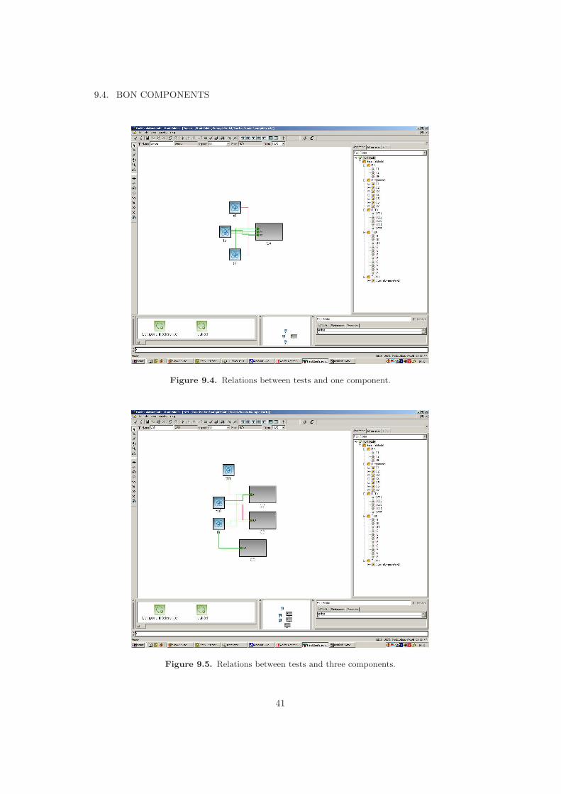
Figure 9.4. Relations between tests and one component.

Figure 9.5. Relations between tests and three components.

41


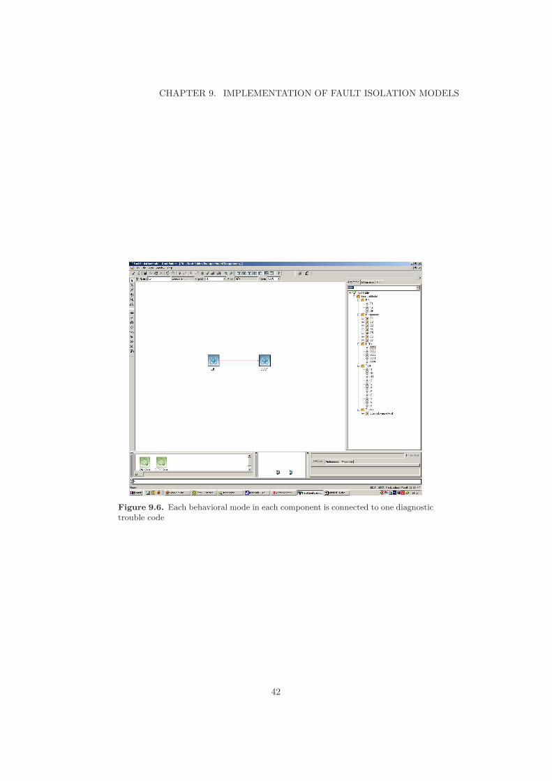
Figure 9.6. Each behavioral mode in each component is connected to one diagnostictrouble code

42

Chapter 10

Exporting model into CSP instance

10.1 Export software

In this thesis a prototype software for exporting information from models createdusing the meta model described in Chapter 8 is developed.

By using the built-in SAX XML-parser in Java the XML file generated by GMEis parsed and a C source file is generated. The C source file describes the CSP usingstructs and arrays in a way that the CSP solver implemented in [5] is able to readthe file as a CSP instance.

The export software mainly consists of six different Java classes:

CSP This class holds the CSP (variables and constraints) we are going to generatefrom the XML File.

Variable Represents a variable and its domain in a CSP.

Constraint Represents a constraint in a CSP. Holds information about includedvariables and the relation between them.

XMLParser Used to parse the XML file from GME. Also some basic search func-tionality is included here.

Element Help class to XMLParser class, representing a single XML element.

Main The Main class.

To verify functionality, the implemented model described in Section 9.2 has beenexported into CSP using the prototype software. These exported CSP instances hasbeen used as input for a CUnit test suite verifying the CSP Solver described in [5].

43

Chapter 11

Conclusions

This thesis forms together with [5] the FJOB diagnosis framework. The frameworkcovers the complete sequence from modeling the system in a modeling environment,with respect to fault isolation, to providing a valid diagnosis at the on-board systemin the vehicle.

The F-JOB diagnosis framework gives the following advantages:

Automated workflow The framework enables good automation of the process.Manual work is mainly done in the Modeling step.

Graphical representation By using a graphical modeling environments a betteroverview of the data is obtained.

Expressiveness Since the CSP Solver is general and many problems can be ex-pressed as CSP, the framework is capable of addressing a large class of prob-lems.

Less manual coding The CSP that should be solved using the CSP Solver is au-tomatically generated by the XML2CSP step. The only manual coding neededis to define how the information defined by the meta model is transformed intoa CSP. Then, for every instance of the meta model, this transformation is au-tomatic.

The modeling part of F-JOB diagnosis framework exemplifies the opportunityto work and structure diagnostic information using a modeling environment, suchas GME.

11.1 Recommendations to Scania

In the long run, go for implementing and use of the F-JOB diagnosis framework.Before the framework can be used in a full way there is a need to make a deeperanalysis of the requirements for the modeling environments.

45

CHAPTER 11. CONCLUSIONS

11.2 Future works

Some areas related to this thesis are recommended for future works. These are:

• Setup a small GME installation and make some real modeling, but in a smalland marked off scope.

• A closer look at the Eclipse based modeling tools, included Topcased. Thisshould include a usability study.

• Extend the meta model described in this work to include more information.

46

Bibliography

[1] Krzystof R. Apt. Principles of Constraint Programming. Cambridge UniversityPress, 2003.

[2] Fahiem Bacchus, Xinguang Chen, Peter Van Beek, and Toby Walsh. Binaryvs. non-binary constraints. Artificial Intelligence, 140:2002, 2002.

[3] Roman Bartak. Constraint satisfaction - heuristics and stochastic algorithms,1998. Accessed 1 December, 2008.

[4] Jonas Biteus. Fault Isolation in Distributed Embedded Systems. PhD thesis,Linköpings universitet, April 2007.

[5] Johan Björling. Fault isolation using wcsp-solver. Master’s thesis, Royal Insti-tute of Technology, June 2009. To appear.

[6] Frank Budinsky, Ed Merks, and David Steinberg. Eclipse Modeling Framework2.0 (2nd Edition). Addison-Wesley Professional, 2008.

[7] Bessiere C. Constraint propagation. In F. Rossi, P. van Beek, and T. Walsh,editors, Handbook of Constraint Programming, chapter 3. Elsevier, 2006.

[8] European Commission. Transport & environment: Road vehicles. http://ec.

europa.eu/environment/air/transport/road.htm, 2009. Accessed 22 May,2009.

[9] World Wide Web Consortium. Extensible markup language (xml). http:

//www.w3.org/XML/, 2009. Accessed 22 May, 2009.

[10] Patrick Farail, Pierre Gaufillet, Agusti Canals, Christophe Le Camus, DavidSciamma, Pierre Michel, Xavier Crégut, and Marc Pantel. the TOPCASEDproject: a toolkit in open source for critical aeronautic systems design. InEmbedded Real Time Software (ERTS), Toulouse, FebruaryMay 2006.

[11] International Organization for Standardization/International Eletrotechni-cal Committee. Information technology – information resource dictionary sys-tem (irds) framework. Technical report, IOS/IEC, 1990.

47

BIBLIOGRAPHY

[12] Mackworth A. K. Freuder E. C. Constraint satisfaction: An emergingparadigm. In F. Rossi, P. van Beek, and T. Walsh, editors, Handbook of Con-straint Programming, chapter 2. Elsevier, 2006.

[13] Akos Ledeczi, Miklos Maroti, Arpad Bakay, Gabor Karsai, Jason Garrett,Chuck Thomasson, Greg Nordstrom, Jonathan Sprinkle, and Peter Volgyesi.The generic modeling environment. In Workshop on Intelligent Signal Process-ing, Budapest, Hungary, May 2001.

[14] Mattias Nyberg and Erik Frisk. Model based diagnosis of technical processes.Linköping University, 2008.

[15] Nikolaos Samaras and Kostas Stergiou. Binary encodings of non-binary con-straint satisfaction problems: Algorithms and experimental results. In Journalof Artificial Intelligence Research 24, 2005.

[16] Douglas C. Schmidt. Guest editor’s introduction: Model-driven engineering.Computer, 39(2):25, 2006.

[17] Ian Sommerville. Software Engineering. Addison-Wesley, Harlow, 8th edition,2007.

[18] Vanderbilt University. GME 7 User’s manual, 2007.

[19] Peter van Beek and Xinguang Chen. CPlan: A constraint programming ap-proach to planning. In AAAI/IAAI, pages 585–590, 1999.

[20] van Beek P. Backtracking search algorithms. In F. Rossi, P. van Beek, andT. Walsh, editors, Handbook of Constraint Programming, chapter 4. Elsevier,2006.

[21] Katriel I. van Hoeve W.-J. Global constraints. In F. Rossi, P. van Beek, andT. Walsh, editors, Handbook of Constraint Programming, chapter 4. Elsevier,2006.

[22] Tim Weilkiens. Systems engineering with SysML/UML : modeling, analysis,design. Morgan Kaufmann OMG Press/Elsevier, Amsterdam, 2008.

48

TRITA-CSC-E 2009:092 ISRN-KTH/CSC/E--09/092--SE

ISSN-1653-5715

www.kth.se

evaluation of modeling environments for managing ... · evaluation of modeling environments for...

Documents