evaluation of production sequencing rules in job shop and ...€¦ · manufacturing companies is...

ID257.1

Evaluation of Production Sequencing Rules in Job Shop and Flow Shop Environment through Computer Simulation

Edna Barbosa da Silva*, Michele Gonçalves Costa*, Marilda Fátima de Souza da Silva*, Fabio Henrique Pereira**

*Diretoria dos Cursos de Informática – Ciência da Computação, Universidade Nove de Julho – Uninove, Av. Francisco Matarazzo 612, 05001100 São Paulo, Brasil, **Programa de Mestrado em Engenharia de Produção

Email: [email protected], [email protected], [email protected], [email protected]

Abstract

In this work, the computational simulation is employed to study the effects of production sequencing rules in the performance of Job Shop and Flow Shop manufacturing environments. Eight sequencing rules have been considered: SIPT (Shortest Imminent Processing Time), EDD (Earliest Due Date), DLS (Dynamic Least Slack), LWQ (Least Work in next Queue), FIFO (First In First Out), LIFO (Last In Last Out), CR (Critical Ratio) and LS (Least Slack). These different sequencing rules was evaluated in relation to the makespan, the total tardiness and number of tardy jobs, considering an experimental scenario which includes two configurations, with 8 machines (processes) and 10 different types of orders. A model of the system was developed in the ARENA® simulation software, taking into account the randomness of the orders arrival profile and of the production times in such environments. The results show that the rules EDD and SIPT have been presented the better performance in the Job Shop and in the Flow Shop environments, respectively.

Keywords: Production Scheduling rules; Manufacturing, Computer Simulation; Job Shop; Flow Shop.

1 Introduction Due to the difficulties faced by the manufacturing companies to improve their productive systems, before priorities quite often conflicting, the simulation has become a widely utilized tool to manage production. One of the main advantages of such technique is to be able of handling bigger problems and in a reasonable computer time, by integrating the diverse system restriction, which can be coupled to the simulation model.

According to Watanabe, Ida and Gen (2005) among the main and hardest problems faced by the flexible manufacturing companies is the production sequencing, also called scheduling, which means to identify the one or the one ways to better ordering the production program in the machines in such a way that they may meet various objectives simultaneously. In this scenario, the environment Job Shop scheduling problem has been extensively studied (Akasawa, 2007; Moreira, 2007; Xu and Zhou, 2009).

The classical Job Shop model addressed in literature shows the following characteristics: a set of n orders {O1, O2, O3,..., On} that has to be processed by m machines {M1, M2, M3,..., Mm} according to p processes {P1, P2, P3…Pp} and some such restrictions thereby: there is a process sequencing, in which each machine processes in its turn, from the start to the end; the processing times can be fixed or variable and the due date may be different (Baptiste, Flamini and Sourd, 2008).

In an attempt to solve this problem, several works have exploited the issue of production sequencing assessing from simple sequencing rules (Montevechi, Turrioni, Almeida, Mergulhão and Leal, 2002; Sims, 1997) up to dynamic systems of rules selection in real time (Mouelhi-Chibani and Pierreval, 2010; Vinod and Sridharan, 2007), in different production environments.

ICIEOM 2012 - Guimarães, Portugal

ID257.2

In fact, a large number of approaches have been reported in the literature to the modeling and solution of these scheduling problems, which include mathematical programming, dispatching rules, neural networks, neighborhood search methods, Petri nets, just to name a few.

In the mathematical programming point of view, formulations using integer programming (Sand and Engell, 2004), mixed-integer programming (Ronconi and Birgin, 2011), and dynamic programming (Ronconi and Powell, 2010) has been extensively applied. However, the use of these approaches to job shop scheduling problems is limited because its computational complexity.

More recently, a large number of new technologies based upon artificial intelligence techniques has been applied to job shop scheduling problems. These include neural network models and neighborhood search methods, such as the tabu search (Hurink, Jurisch and Thole, 1994), simulated annealing (Jeffcoat and Bulfin, 1993) and genetic algorithms (Buzzo and Moccellin, 2000). Although these methods are very popular and provide good feasible solutions, they have some serious disadvantages as the lack of optimality criteria and the computational cost.

Other important kind of methods that stands for many contributions in the modeling and simulation of production scheduling and routing is the formalism of Petri nets. Petri nets addresses the issue of flexibility which is frequently discards in effective algorithms for scheduling problems (Aalst, 1992). Extensions of this approach, which typically are the addition of ‘colour’, ‘time’ and ‘hierarchy’ (Bai, Zhang and Zhang, 2005; Zhang and Gu, 2009), have been proposed to modelling of complex systems with very good results. In fact, according to Zhang and Gu (2009), comparison with some previous approaches shows that the timed Petri nets model is more compact and effective in finding the best solution in practical job shop scheduling problems.

Finally, simple sequencing rules based on information related to the jobs as, for example, processing times e due dates, also have been applied consistently to scheduling problems, mainly designed to provide good and fast solutions to complex problems (Jones and Rabelo, 1998).

It is highlighted here the work designed by Santoro and Mesquita (2008), which addresses the problem of Job Shop environment production sequencing, in which the orders stick to a route specific and pre-determined. A simulation model created on Visual Basic for Applications (VBA) in Excel spreadsheets, was used to evaluate the effect of the work in process in relation to the total tardiness and the total number of tardy orders, making it possible to conclude that it is possible to decrease the total tardiness and the total number of tardy orders and, even so, to keep the intermediate stocks at a constant volume.

The production scenario used by those authors made up of two distinctive production environments, was the grounding for this work. However, instead of considering that all orders are available for production input in the system at the instant Zero (0), this work takes into account the randomness of the time between arrivals of the orders, which reflects the intent of simulating a flexible manufacturing environment with a high products mix alongside lots tending to the unity.

Indeed, simulation has been one of the most utilized tool in the manufacturing area once it provides means to identify, analyze and improve the parameters of production and process such as: analysis of machinery and operators; processing time; evaluation of operational performance and procedures as well as to assess the production sequencing and production flow, allowing for the knowledge of the points where the system permits a broader production flexibility (Costa and Jungles, 2006; Pontes, Yamada and Porto, 2007).

In accordance with which has been pointed out by Chwif and Medina (2006), the use of computer simulation makes it possible to predict with a certain degree of assurance and meeting a set of assumptions, the behavior of a system holding a database of specific input elements. In this work computer simulation is used to study the effect of the production sequencing rules over the performance of a Job Shop manufacturing environment, whose process allows the production orders to move from a workstation to another, according to the pre-determined production sequencing, and in a Flow Shop environment, in which the process permits that the production orders go to just one workstation ahead.

Evaluation of Production Sequencing Rules in Job Shop and Flow Shop Environment

through Computer Simulation

ID257.3

Herein, eight sequencing rules are addressed and evaluated with regards to the completion time of a schedule (makespan), total tardiness time and the average number of tardy orders, taking into consideration an experimental scenario, which comprises two settings of work environment with 8 machines (processes) and 10 different type of orders. A model of the system was developed on the simulation software ARENA®, featuring the random behavior of the orders arrival and the production times in this kind of environment. The obtained results show that the EDD and SIPT rules yield the best performance at Job Shop and Flow Shop environments, respectively.

2 Production Sequencing Rules Production sequencing rules, which are also called production scheduling and dispatching rules, are understood as being the event of orders arrival, pieces and tasks of the system. The sequencing rules are normally classified in different classes according to the performance criteria for which they have been developed (Wu, 1987). The first of these classes contains simple rules designed mainly to provide good and fast solutions to complex problems (Jones and Rabelo, 1998). These rules are based on information related to the jobs, such as processing times e due dates, and have been applied consistently to scheduling problems.

The sequencing rules can be also classified as local or global rules (Reid and Sander, 2005). The local rules establishes priorities based only on orders that are waiting at a specific workstation. Global rules, on the other hand, consider factors related to all workstations on the orders route. The rule Least Work Next Queue (LWQ) is an example of a global sequencing rule in which the priority is given to the task heading to the machine or workstation with the smallest queue.

Overall, the simulation approach has been extensively used to study the performance of these rules. Start from Conway and Maxwell (1967), who were the first to study the Shortest Processing Time rule (SPT) and its variations, a lot of works have been carried out to find the best choice for optimizing different performance measures.

The main dispatching rules adapted from Mesquita et al. in Lustosa et al. (2008), Tubino (2007), Suresh and Sridharan (2007), Chan and Chan, (2004) and Gaither and Frazier (2002), can be defined as it follows:

FIFO – (First In, First Out) Priority is given to the first piece that is input, which must be the first to be output. It can be taken as an arrival order into the machine in the factory. This rule seeks to minimize the time of staying on the machine or in the factory.

LIFO – (Last In, First Out) Priority is given to the last piece that is input, which is the first to be output. Due to the fact of it being adverse and negative with regards to reliability and quickness to deliver and for not having a sequencing based on quality, flexibility or cost, this rule is used hardly ever.

SPT – (Shortest Processing Time) Priority is given to the shortest total processing time. It is classified in an ascending time order. Its use is aimed at reducing the size of the queues and the increasing of the flow.

LPT – (Longest Processing Time) Priority is given to the longest total processing time. It is conversely to the SPT rule. Its utilization focus on reducing the changes of machines.

EDD – (Earliest Due Date) Priority is given to the fulfillment of the most urgent orders in terms of delivery deadline. The main purpose is to reduce tardiness.

LS – (Least Slack) Priority is given to the shortest slack between the due date and the total processing time among the tasks that are in queue. It is classified by delivery deadline and focus on reducing tardiness.

SIPT – (Shortest Imminent Processing Time) Priority is given to shortest individual processing time. SIPT and SPT are alike.


ID257.4

LIPT – (Longest Imminent Processing Time) Priority is given to the longest individual processing time. LIPT and LPT are alike.

LWQ – (Least Work Next Queue) Priority is given to the task heading to the machine or workstation with the smallest queue. This rule is targeted at avoiding the stall of a subsequent process.

CR – (Critical Ratio) Priority is given to the smallest critical ratio (time span until the expiring date divided by the total production remaining time) between the tasks in queue. This is a dynamic rule, which seeks to combine EDD with SPT, that relies solely on the processing time.

DLS – (Dynamic Least Slack) Priority is given to the least slack (difference between the estimated date of delivery and the total processing remaining time). This rule gives priority to the most urgent tasks with the purpose of reducing tardiness. However, it is a little bit more complex to implement than LS because it is a dynamic rule.

In fact, there are numerous objectives in scheduling and, therefore, there are dozens of sensible performance measures which are complex and often conflicting. So, in order to evaluate the impact of the sequencing rules on the manufacturing performance specific performance measure must be considered. This issue is addressed in next section.

3 Performance Indexes In order to measure the efficacy of a decision, we lay hands on performance indexes. Each objective outlined by the company is attached to a measure of performance, which in its turn, is connected to one or more performance indexes. In general, these measures can be grouped in two categories: (i) the job-related performance measures, such as due date and tardiness, which are indicative of customer satisfaction and deliverability; and (ii) the shop-related measures, such as earliness, mean total time in the system, mean queue time in the shop-floor and machine utilization . The most common indexes according (Gaither and Frazier, 2002; Reid and Sanders, 2005; Arenales et all., 2007), are:

Flow average time or follow through (Makespan): the average between the orders flow time. This index is related to the operating efficiency indicating the time required to execute a set of N orders.

Average tardiness or maximum tardiness: the average of the tardiness or longest tardiness between the orders appraised.

Work total time: the time interval between the release of the first operation of the first order and the ending of the last process of the last order.

Average of the work in process: the average of the number of open orders and not finished yet. Number of tardy orders: the number of orders that were not delivered to the customer on due

time. Tardiness total time: it is the sum of all the times of all orders that have been tardy.

In general, the performance measures are often conflicting and the optimization of more than one criterion must take into account the trade-off characterized by a multiple objectives optimization (Arenales et al., 2007).

4 Modeling and Simulation Computer simulation refers to the methods to study various real or artificial models on numerical evaluation systems using softwares designed to mock an operation system and/or characteristics usually



ID257.5

over a period of time. In practice, it means that it is a creation process of computerized model intended to carry out numerical trials, in such a way, to foster the understanding of this system, subjected to a certain set of conditions (Kelton, Sadowski and Sadowski, 2000).

In order to develop a simulation model it is necessary take into account a few procedures to ensure that it can predict the behavior of a system with some confidence, and respect a set of assumptions, based on specific input data (Chwif and Medina, 2006). These procedures can be divided into four major steps: (i) Planning Stage, which includes the formulation and analysis of the problem, project planning, conceptual model formulation and macro collection of information; (ii) Modeling stage, formed by the data collection, the computational implementation, verification and validation of the model. (iii) stage of experimentation and statistical analysis of data, and (iv) the last step in which the best solutions are compared and identified, and the results are presented (Freitas Filho, 2008).

Working with a larger variety of scientific models than the mathematical analysis, computer simulation is used in cases where the models or problems are highly complex for formal mathematical analysis (Bertrand and Fransoo, 2002). It cannot be taken as a mathematical model, though it employs mathematical formulas in the quest for solutions to the various systems. It cannot be mistaken for an optimization technique because it is a tool for the scenarios analysis, however, it can be coupled with optimization algorithms to figure out better solutions.

The simulation softwares work basically set on graphical interfaces, where the user can use it in an intuitive manner through graphical menus and chat boxes. The possibility of building models run with animations may make it easy to understand the system once they allow to add movements which change their dynamics.

Alongside simulation softwares, there are simulation languages that make up a set of one or more programs designed for the most specific applications. Its main advantage is to pave the way for the generation of the most varied type of systems. Notwithstanding, they require that the users have a deep knowledge of this type of language, so they may be able to bring forth more complex systems.

5 Model Description The simulation model was built based on the production scenarios configured by Santoro and Mesquita (2008), made up of 8 machines and 10 types of orders with pre-established routes and production total times determine according to Table 1. It was chosen to mock a production type of Job Shop and Flow Shop environments. The starting conditions for the simulation model proposed were:

Each machine is always available, that is, temporary unavailability caused by breaking down, maintenance or set ups, or for whatsoever reason, were not considered;

Once a production process of an order gets started on a machine it cannot be stopped; When the execution of a task on a machine is finished, it is sent automatically to the next without

considering eventual transport time; There is no operations overlapping; The orders are fulfilled independently of one another; For the purpose of keeping a ratio, it was determined that the deployment likelihood of each one

of the 10 order types is 10%.

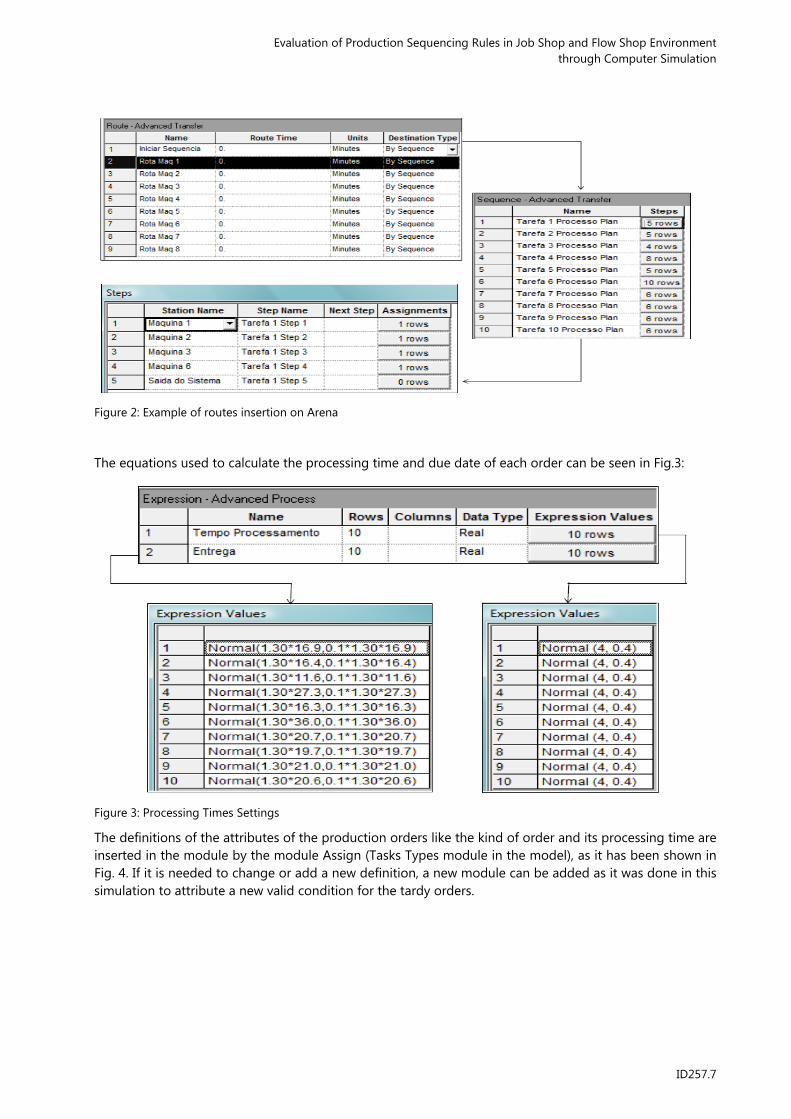
The same parameters were also utilized to generate the delivery date, yielded by Normal distribution of (1+k) *t0 average and 0.1* (1+k)*t0’ standard deviation, where t0 is the production total time and k is a confidence factor with regards to this time. To this situation, it was used a 30% fixed value for the confidence factor. As an example of a formula loaded into Arena®, we have: Normal (1.30*16.9;0.1*1.30*16.9), where 16.9 is the total time of the first order in accordance with Table 1. The base-scenario employed assumed that all the orders were available to be input into production in the system at the instant Zero (0); however, in this work modeling, the time intervals between the arrival of


ID257.6

the orders were randomized and described for an exponential distribution of 11 minutes average. The choice makes evident the intention of simulating an environment of flexible manufacturing holding a high mix of products alongside lots tending to the unity.

Table 1: Estimated time and route data

Job Shop Routes Flow Shop Routes # Route Time # Route Time

1 1,2,3,6 16.9 1 1,3,5,6 15.5 2 1,3,7,8 16.4 2 2,3,4,5,6,8 25.6 3 1,5,8 11.6 3 1,3,4,7,8 20.3 4 1,2,3,5,6,7,8 27.3 4 3,4,5,7,8 20.9 5 3,4,6,7 16.3 5 1,2,3,5,6,7,8 26.5 6 1,2,4,3,1,2,4,5,7 36.0 6 1,2,3,5,7 19.8 7 2,6,5,6,8 20.7 7 1,2,3,4,5,7 24.5 8 1,2,4,5,7 19.7 8 1,3,5,6,8 19.8 9 2,3,4,6,7 21.0 9 2,4,6,7,8 19.1 10 1.2.4.5.8 20.6 10 3.4.5.6.7 20.1

Source: Santoro e Mesquita, 2008, p.81

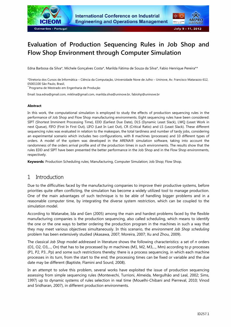
Figure 1 shows a simulation model developed, where the Process Maq i modules can be identified, which represent each one of the 8 machines of the environment studied, followed by the module that informs the route of each order upon going through the machine. The first route is identified in the Tasks Launching Station (Lanc de Tarefas).

After the Exit the System Station, are the modules related to the performance of each one of the sequencing rules of the production orders as well as the modules which register the storing of the results.

Figure 1: Developed Simulation Model

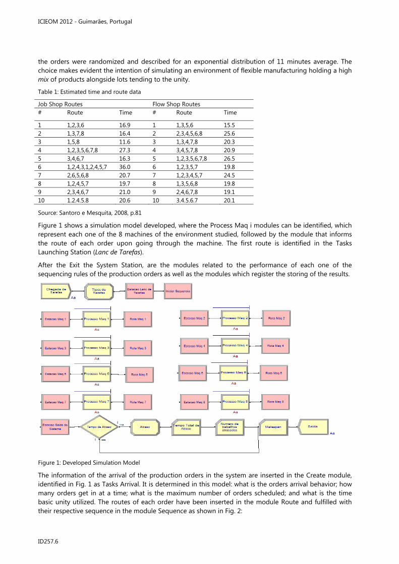
The information of the arrival of the production orders in the system are inserted in the Create module, identified in Fig. 1 as Tasks Arrival. It is determined in this model: what is the orders arrival behavior; how many orders get in at a time; what is the maximum number of orders scheduled; and what is the time basic unity utilized. The routes of each order have been inserted in the module Route and fulfilled with their respective sequence in the module Sequence as shown in Fig. 2:



ID257.7

Figure 2: Example of routes insertion on Arena

The equations used to calculate the processing time and due date of each order can be seen in Fig.3:

Figure 3: Processing Times Settings

The definitions of the attributes of the production orders like the kind of order and its processing time are inserted in the module by the module Assign (Tasks Types module in the model), as it has been shown in Fig. 4. If it is needed to change or add a new definition, a new module can be added as it was done in this simulation to attribute a new valid condition for the tardy orders.


ID257.8

Figure 4: Production Orders Attributes Definitions

The information needed for the simulator to identify which sequencing rules must be followed by the orders in conformity with the route assigned to in each machine are defined according to Fig. 5:

Figure 5: Identification of the simulated sequencing order

6 Results 20 replications with 1,000 minutes each were considered. The number of replications was validated by data analysis with 95% confidence for each run. The quantity of minutes used is sufficient to meet the time the simulation needs to enter the period of stability. A system is said to be stable when the production process gets into permanent regime and eventual variations caused by start-up have already been ruled out.

The results obtained from the simulation model are graphically shown below. Taken into account the measures related to performance (Makespan, Tardiness Total Time, and the Number of Tardy Orders) and setting up of the two environments (Job Shop and Flow Shop), these results are presented into two subsections. Each subsection displays a brief analysis of the results achieved.

6.1 Job Shop Environment For this environment, the performance measures are presented in Fig. 6, 7 and 8 to Tardiness Total Time, Number of Tardy Orders and Makespan, respectively.



ID257.9

Figure 6: Total Tardiness – Job Shop

Figure 7: Number of Tardy Orders – Job Shop

Figure 8: Makespan – Job Shop

In accordance with Fig. 6, 7 and 8, in the Job Shop environment, the sequencing rules which presented the best performance, were EDD and LIFO. The performance indicators Makespan and Tardiness Total Time, shown better results with the EDD rule; nevertheless, the Number of Tardy Orders presented a better performance under the LIFO rule. When making use of the 95% confidence interval, the following margin errors were shown: 0.18 to Makespan (EDD), 99.8 to Tardiness Total Time (EDD) and 10.66 to the Number of Tardy Orders (LIFO).


ID257.10

6.2 Flow Shop Environment For this environment, the performance measures were displayed in Fig. 9, 10 and 11 for Tardiness Total Time, Number of Tardy Orders and Makespan, respectively.

Figure 9: Tardiness Total Time – Flow Shop

Figure 10: Number of Tardy Orders – Flow Shop

Figure 11: Makespan – Flow Shop

In accordance with Fig. 9, 10 and 11, in the Flow Shop environment, the SIPT sequencing rule presented the best performance for the three indicators.

24.6 24.5 24.4 24.3



ID257.11

The following margin errors were shown, using the 95% confidence interval: 0.22 to Makespan (SIPT), 121.61 to Tardiness Total Time (EDD) and 9.54 to Number of Tardy Orders.

7 Conclusion First of all, it is necessary to consider which of the performance indicators are the most outstanding ones when choosing the work order sequencing. The results analysis, considering the Tardiness Total Time with the most important indicator, shows that, in Flow Shop environment, the SIPT rule presents better results in relation to the other rules. Nevertheless, in Job Shop environments the best result was shown by the EDD rule. Considering Makespan the most important indicator, the EDD rule, once again, presents a better result in Job Shop environments. In Flow Shop environments, SIPT and CR rules showed results alike. Taking into account the Number of Tardy Orders as the most important indicator, the LIFO rule, presented better result in Jop Shop environments. In Flow Shop environments the best result was shown under SIPT rule. The results demonstrate that the sequencing rules should be applied to in accordance with the environment and the indicators significance. It is worth pointing out that, despite the developed model assumes a hypothetical production scenario, it can be easily adjusted to a real environment by changing properly the number of workstations and adjusting the distributions of the orders arrival likelihood and processing times by means of data collecting. These adjustments can be easily carried out in the modules that have been presented in Fig. 3, 4 and 5.

Finally, it is made evident that the observing of the randomness of the arrivals and the production times may reflect more appropriately the reality of manufacturing environments, in which, the demand, is characterized by a high mix of products and lots, whose sizes, tend to the unity.

Acknowledgments Authors would like to thank Nove de Julho University- Uninove for the financial support.

References Aalst, W. M. P. Van Der (1992). Timed coloured Petri nets and their application to logistics, Ph.D. thesis, Eindhoven

University of Technology, Eindhoven. Aalst, W. M. P. Van Der (1993), Interval Timed Coloured Petri Nets and their Analysis, in: M. Ajmone Marsan (ed.),

Application and Theory of Petri Nets 1993, Lecture Notes in Computer Science 691, Springer-Verlag, Berlin, p.453–472.

Akasawa, A. (2007). Aplicação da Simulação de Eventos Discretos como ferramenta integrada ao planejamento e programação daprodução na manufatura ágil. Itajubá, 118p. Dissertação (Mestrado em Ciências em Engenharia de Produção) Universidade Federal de Itajubá. Minas Gerais.

Arenales, M.; Armentano, V.; Morabito, R.; Yanasse, H. (2007). Pesquisa Operacional. Rio de Janeiro: Elsevier. Bai, Q; Zhang, M.; Zhang, H. (2005). A Coloured Petri Net Based Strategy for Multi-Agent Scheduling. Proceedings of the

Rational, Robust, and Secure Negotiation Mechanisms in Multi-Agent Systems (RRS'05), p. 3-10. Baptiste, P.; Flamini, M.; Sourd, F. (2008) Lagrangian bounds for just-in-time job-shop scheduling. Computers &

Operations Research, v. 35, n. 3, p. 906-915. Bertrand, J. W. M.; Fransoo, J. C. (2002). Modelling and simulation Operations Management research methodologies quantitative modeling. International Journal of Operations and Production Management, v.22, n.2, p.241-261.

Buzzo, W. R.; Moccellin, J. V. (2000). Programação da produção em sistemas flow shop utilizando um método heurístico híbrido algoritmo genético-simulated annealing. Gest. Prod., v.7, n.3, p.364-377.

Chan, F. T. S.; Chan, H. K. (2004). Analysis of dynamic control strategies of an FMS under different scenarios. Robotics and Computer-Integrated Manufacturing, n. 20, p. 423–437.

Chwif, L.; Medina, A. C. (2006). Modelagem e Simulação de Eventos Discretos: Teoria e Aplicações. 2ª ed. São Paulo, Gráfica Palas Athena.

Conway, R.; Maxwell, W. (1967). Theory of Scheduling. Reading, Massachusetts: Addison-Wesley.


ID257.12

Costa, A. C. F.; Jungles, A. E. (09 a 11 de outubro 2006). O Mapeamento do Fluxo de Valor Aplicado a uma Fábrica de Montagem de Canetas Simulada. In: XXVI Encontro Nacional de Engenharia de Produção. Fortaleza, CE, Brasil.

Freitas Filho, P. J. (2008). Introdução à modelagem e simulação de sistemas. 2ª ed. P 372, Florianópolis, Visual Books. Gaither, N.; Frazier, G. (2002). Administração da Produção e Operações. 8. ed. São Paulo, Pioneira. Hurink, J. L.; Jurisch, B.; Thole, M. (1994). Tabu search for the job-shop scheduling problem with multi-purpose

machines. OR Spectrum, v.15, n.4, p.205-215. Jeffcoat, D.; Bulfin, R. (1993). Simulated annealing for resource-constrained scheduling. European Journal of

Operational Research, v.70, p.43-51. Jones, A.; Rabelo, L. C. (1998). Survey of Job Shop Scheduling Techniques. In: http://citeseer.nj.nec.com. Kelton, W. D.; Sadowski, R., P.; Sadowski, D. A. (2000). Simulation With ARENA, 2ª ed. McGraw Hill. Mesquita, M.; Costa, H. G.; Lustosa, L.; Silva, A. S. (2008). Programação detalhada da produção. In: Lustosa, L. J.;

Mesquita, M. A.; Quelhas, O.; Oliveira, R. Planejamento e Controle da Produção. Rio de Janeiro: Elsevier. Montevechi, J. A. B.; Turrioni, J. B.; Almeida, D. A.; Mergulhão, R. C.; Leal, F. (2002). Análise comparativa entre regras

heurísticas de sequenciamento da produção aplicada em job shop. Produto & Produção, v.6, n.2, p.12-18. Moreira, M. R. (2007). Controlo input-output em job-shops: Como as regras de decisões interagem e reagem a falhas

nas máquinas. In: XVII Jornadas Hispano-Lusas de Gestión Científica - Conocimiento, Innovación y Emprendedores: Caminho al Futuro, p. 2257-2569.

Mouelhi-Chibani, W., Pierreval, H. (2010). Training a neural network to select dispatching rules in real time. Computers & Industrial Engineering, v.58, n.2, 249-256.

Pontes, H. L. J. ; Yamada, M. C.; Porto, A. J. V. (2007). Análise do arranjo físico de uma linha de montagem em uma empresa do setor de componentes automotivos utilizando simulação. In: 8o Congresso Ibero Americano de Engenharia Mecânica. Cuzco, Peru.

Reid, R. D.; Sanders, N. R. (2005). Gestão de Operações. Rio de Janeiro: LTC. Ronconi D. P.; Birgin E. G. Mixed-Integer Programming Models for Flowshop Scheduling Problems Minimizing the Total

Earliness and Tardiness, in Just-in-Time Systems, Y.A. Ríos-Solís and R.Z. Ríos-Mercado (Eds.), Springer Series on Optimization and Its Applications, P.M. Pardalos and Ding-Zhu Du (Series eds.), to appear.

Ronconi, D. P.; Powell, W. B. (2010). Minimizing Total Tardiness in a Stochastic Single Machine Scheduling Problem using Approximate Dynamic Programming. Journal of Scheduling, v.13, p. 597-607.

Sand, G.; Engell, S. (2004). Modeling and solving real-time scheduling problems by stochastic integer programming. Computers and Chemical Engineering, v.28, p.1087–1103.

Santoro, M. C.; Mesquita, M. A. (2008). The effect of the workload on due-date performance in job shop scheduling. Brazilian Journal of Operations and Production Management, v. 5, p. 75-88.

Sims, M.J. (1997). An introduction to planning and scheduling with simulation. In Proceedings of the 1997 Winter Simulation Conference, Atlanta, GA, p. 67-69.

Sousa, P. S. A.; Moreira, M. R. A. (2007). Performance Analysis of Job-Shop Production Systems under Different Order Release Control Parameters. Proceedings of the World Congress on Engineering, WCE 2007, London, U.K.

Suresh, K.N.; Sridharan, R. (2007). Simulation modeling and analysis of tool sharing and part Scheduling decisions in single-stage multimachine flexible manufacturing systems. Robotics and Computer-Integrated Manufacturing, n. 23, p. 361-370.

Tubino, D. F. (2007). Planejamento e Controle da Produção: Teoria e Prática. São Paulo, Atlas. . Vinod, V.; Sridharan, R. (2008).Scheduling a dynamic job shop production system with sequence-dependent setups.

Robotics and Computer-Integrated Manufacturing, p. 435-449. Watanabe, M.; Ida, K.; Gen, M. A. (2005). genetic algorithm with modified crossover operator and search area

adaptation for the job-shop scheduling problem. Computers & Industrial Engineering, n. 48 p. 743-752. Wu, D. (1987). An Expert Systems Approach for the Control and Scheduling of Flexible Manufacturing Systems. Ph.D.

Dissertation, Pennsylvania State University. Xu, J.; Zhou, X. A. (2009). class of multi-objective expected value decision-making model with birandom coefficients

and its application to flow shop scheduling problem. Information Sciences, n. 179, p. 2997-3017. Zhang, H.; Gu, M. (2009). Modeling jobshop scheduling with batches and setup times by timed Petrinets.

Mathematical and Computer Modelling, v.49, n.1–2, p.286–294.

evaluation of production sequencing rules in job shop and ...€¦ · manufacturing companies is...

Documents