evaluation of spring discharge for characterization of
TRANSCRIPT

Evaluation of Spring Discharge for Characterization of Groundwater Flow in
Fractured Rock Aquifers: A Case Study from the Blue Ridge Province, VA
W. Miles Gentry
Thesis submitted to the Faculty of Virginia Polytechnic Institute and State University in
partial fulfillment of the requirements for the degree of
MASTER OF SCIENCE
In
GEOLOGICAL SCIENCES
Thomas J. Burbey (Chair)
Madeline Schreiber
John A. Hole
Virginia Polytechnic Institute and State University,
Blacksburg, VA
Keywords: Blue Ridge, Springflow, Fractured Rocks, Springs
Copyright 2003, W. Miles Gentry

Evaluation of Spring Discharge for Characterization of Groundwater Flow in
Fractured Rock Aquifers: A Case Study from the Blue Ridge Province, VA
W. Miles Gentry
Abstract
Recent models of groundwater flow in the Blue Ridge Province suggest multiple
aquifers and flow paths may be responsible for springs and seeps appearing throughout
the region. Deep confined aquifers and shallow variably confined aquifers may
contribute water to spring outlets, resulting in vastly different water quality and
suitability for potable water supplies and stock watering. A new Low Flow Recording
System (LoFRS) was developed to measure the discharge of these springs that are so
ubiquitous throughout the Blue Ridge Province.
Analysis of spring discharge, combined with electrical resistivity surveying,
aquifer tests, and water chemistry data reveal mixed shallow and deep aquifer sources for
some springs, while other springs and artesian wells are sourced only in the deep aquifer.
The technique is suitable for rapid characterization of flow paths leading to spring outlets.
Rapid characterization is important for evaluation of potential water quality problems
arising from contamination of shallow and deep aquifers, and for evaluation of water
resource susceptibility to drought. The spring discharge technique is also suitable for use
in other locations where fractured rock and crystalline rock aquifers are common.

iii
Acknowledgements
I would like to thank everyone involved in this project for contributing directly, or
indirectly to its completion. My principal advisor, Tom Burbey, provided funding,
insight, and occasional golf lessons that all helped greatly with the completion of this
study. Madeline Schreiber provided constant suggestions for improvement of my field
methods and equipment (some of which are still under development) and somehow
managed to persuade me into building more field equipment for her projects. John Hole
endowed me with the ability to survive any academic hardship (be it potential fields class
or inversion theory class).
I would also like to thank my friends who have each contributed in their own ways to this
project:
My parents who have kept me awash in food and inspiration through this whole project.
Gini, Scottie and Bucky Pritchard who allowed me to use their Grayson County property
as a second field site, Jackson and Jay who always suggested it was time to go fishing
instead of time to do research, Bill Seaton for research and geologic insight throughout
the project, and in no particular order: Bill Henika, K.C. St.Clair, Isaac Jeng, Karen
Weber, Lauren Velander, Rob Lawson, Stacie Dunkle, Susan and Kelly Mattingly, Rance
Edwards, Jennifer Stempien, and the entire Carbonate Lab.
Finally, a special thanks to Connie Lowe, our departmental student coordinator, who
somehow manages to keep up with 45+ grad students, numerous undergrads, and all of
our successes and problems.

iv
Table of Contents
ABSTRACT...................................................................................................................... II
ACKNOWLEDGEMENTS ...........................................................................................III
LIST OF TABLES..........................................................................................................VI
BACKGROUND ............................................................................................................... 1
OBJECTIVES OF THIS INVESTIGATION ................................................................ 7
GEOLOGY, PHYSIOGRAPHY, AND GEOMORPHOLOGY .................................. 7 FLOYD COUNTY FIELD SITE DESCRIPTION..................................................................... 10 GRAYSON COUNTY FIELD SITE DESCRIPTION................................................................ 11
CLIMATE ....................................................................................................................... 14
HYDROGEOLOGY....................................................................................................... 15 Previous Work........................................................................................................... 15 Evidence of Multiple Flow Regimes ......................................................................... 17 CFC Data.................................................................................................................. 17 Well Log Data ........................................................................................................... 18 Chemistry .................................................................................................................. 19 Spring Observations.................................................................................................. 22 Spring Discharge Measurements and Their Correlation to Rain Events ................. 22 Determination of Recession Curve Parameters and Flow Paths ............................. 31 Resistivity Characterization of Geology and Hydrology .......................................... 34 Resistivity Techniques and Interpretation ................................................................ 35 Aquifer Tests ............................................................................................................. 45
APPLICATIONS TO OTHER LOCATIONS............................................................. 51
SUMMARY AND CONCLUSIONS ............................................................................. 60
APPENDIX I – SCHEMATIC DIAGRAM OF DISCHARGE MEASUREMENT SYSTEM .......................................................................................................................... 64
APPENDIX II – DIPOLE-DIPOLE ARRAY DETAILS............................................ 66
APPENDIX III – RESISTIVITY INVERSION PARAMETERS.............................. 68
VITA ................................................................................................................................ 70
v
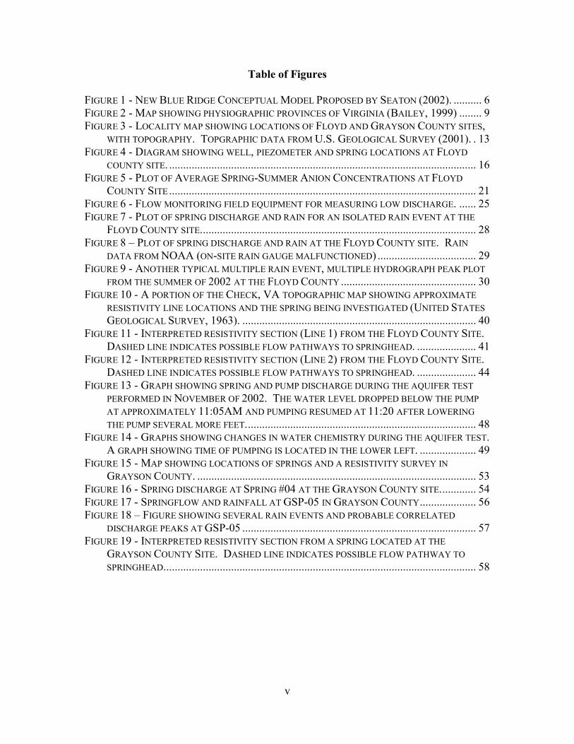
Table of Figures
FIGURE 1 - NEW BLUE RIDGE CONCEPTUAL MODEL PROPOSED BY SEATON (2002). .......... 6 FIGURE 2 - MAP SHOWING PHYSIOGRAPHIC PROVINCES OF VIRGINIA (BAILEY, 1999) ........ 9 FIGURE 3 - LOCALITY MAP SHOWING LOCATIONS OF FLOYD AND GRAYSON COUNTY SITES,
WITH TOPOGRAPHY. TOPGRAPHIC DATA FROM U.S. GEOLOGICAL SURVEY (2001). . 13 FIGURE 4 - DIAGRAM SHOWING WELL, PIEZOMETER AND SPRING LOCATIONS AT FLOYD
COUNTY SITE. ............................................................................................................. 16 FIGURE 5 - PLOT OF AVERAGE SPRING-SUMMER ANION CONCENTRATIONS AT FLOYD
COUNTY SITE ............................................................................................................. 21 FIGURE 6 - FLOW MONITORING FIELD EQUIPMENT FOR MEASURING LOW DISCHARGE. ...... 25 FIGURE 7 - PLOT OF SPRING DISCHARGE AND RAIN FOR AN ISOLATED RAIN EVENT AT THE
FLOYD COUNTY SITE.................................................................................................. 28 FIGURE 8 – PLOT OF SPRING DISCHARGE AND RAIN AT THE FLOYD COUNTY SITE. RAIN
DATA FROM NOAA (ON-SITE RAIN GAUGE MALFUNCTIONED) ................................... 29 FIGURE 9 - ANOTHER TYPICAL MULTIPLE RAIN EVENT, MULTIPLE HYDROGRAPH PEAK PLOT
FROM THE SUMMER OF 2002 AT THE FLOYD COUNTY ................................................ 30 FIGURE 10 - A PORTION OF THE CHECK, VA TOPOGRAPHIC MAP SHOWING APPROXIMATE
RESISTIVITY LINE LOCATIONS AND THE SPRING BEING INVESTIGATED (UNITED STATES GEOLOGICAL SURVEY, 1963). ................................................................................... 40
FIGURE 11 - INTERPRETED RESISTIVITY SECTION (LINE 1) FROM THE FLOYD COUNTY SITE. DASHED LINE INDICATES POSSIBLE FLOW PATHWAYS TO SPRINGHEAD. ..................... 41
FIGURE 12 - INTERPRETED RESISTIVITY SECTION (LINE 2) FROM THE FLOYD COUNTY SITE. DASHED LINE INDICATES POSSIBLE FLOW PATHWAYS TO SPRINGHEAD. ..................... 44
FIGURE 13 - GRAPH SHOWING SPRING AND PUMP DISCHARGE DURING THE AQUIFER TEST PERFORMED IN NOVEMBER OF 2002. THE WATER LEVEL DROPPED BELOW THE PUMP AT APPROXIMATELY 11:05AM AND PUMPING RESUMED AT 11:20 AFTER LOWERING THE PUMP SEVERAL MORE FEET.................................................................................. 48
FIGURE 14 - GRAPHS SHOWING CHANGES IN WATER CHEMISTRY DURING THE AQUIFER TEST. A GRAPH SHOWING TIME OF PUMPING IS LOCATED IN THE LOWER LEFT. .................... 49
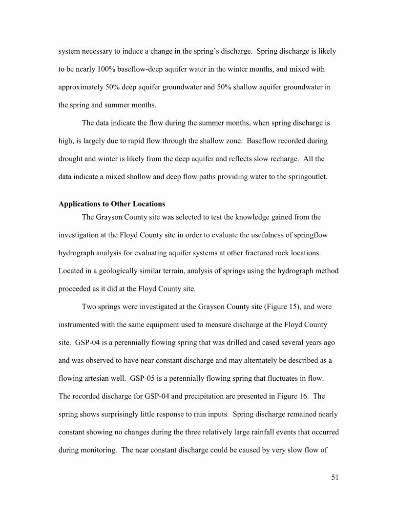
FIGURE 15 - MAP SHOWING LOCATIONS OF SPRINGS AND A RESISTIVITY SURVEY IN GRAYSON COUNTY. ................................................................................................... 53
FIGURE 16 - SPRING DISCHARGE AT SPRING #04 AT THE GRAYSON COUNTY SITE............. 54 FIGURE 17 - SPRINGFLOW AND RAINFALL AT GSP-05 IN GRAYSON COUNTY.................... 56 FIGURE 18 – FIGURE SHOWING SEVERAL RAIN EVENTS AND PROBABLE CORRELATED
DISCHARGE PEAKS AT GSP-05 ................................................................................... 57 FIGURE 19 - INTERPRETED RESISTIVITY SECTION FROM A SPRING LOCATED AT THE
GRAYSON COUNTY SITE. DASHED LINE INDICATES POSSIBLE FLOW PATHWAY TO SPRINGHEAD............................................................................................................... 58

vi
List of Tables
TABLE 1 - WATER SOURCES FOR FLOYD, GRAYSON AND WARREN COUNTIES, VIRGINIA.
DATA FROM U.S. CENSUS BUREAU, 1990. .................................................................. 1 TABLE 2 - SPRING DISCHARGE MONITORING PERIODS........................................................ 24 TABLE 3 -TABLE SHOWING CALCULATED RECESSION ALPHA VALUES AND COMPARISON
VALUES. MIDDLE EAST VALUES FROM AMIT, ET AL. (2002)..................................... 32
1
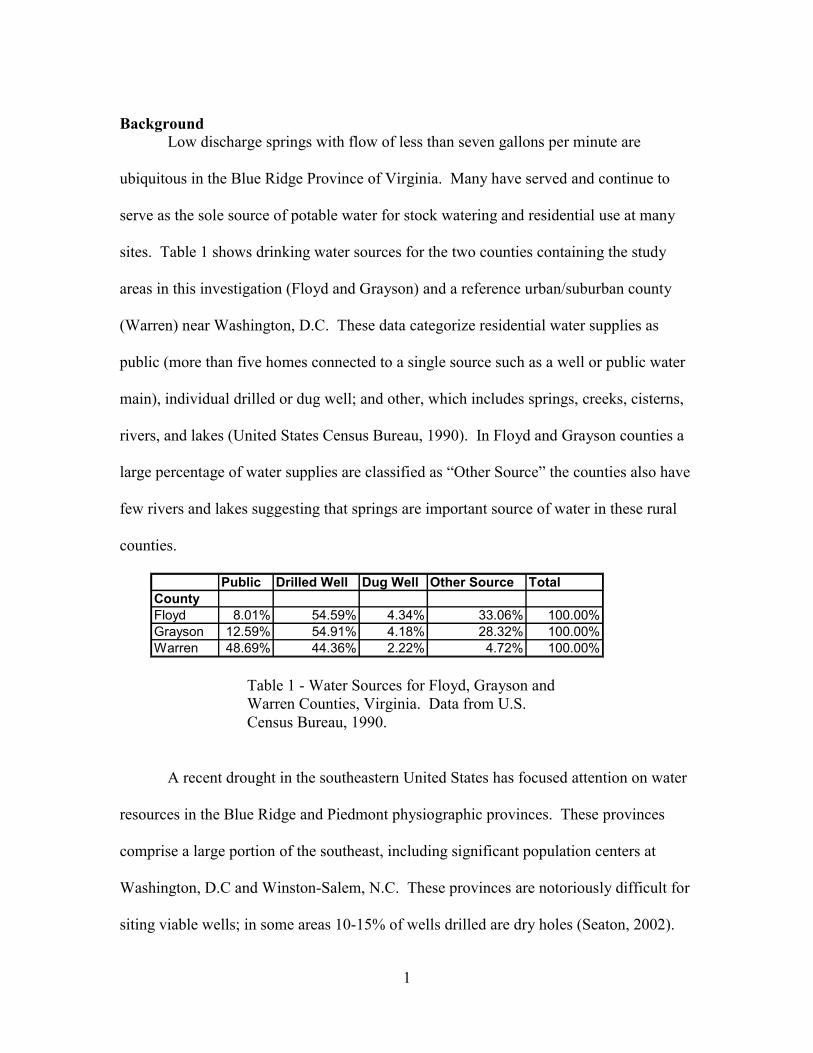
Background Low discharge springs with flow of less than seven gallons per minute are
ubiquitous in the Blue Ridge Province of Virginia. Many have served and continue to
serve as the sole source of potable water for stock watering and residential use at many
sites. Table 1 shows drinking water sources for the two counties containing the study
areas in this investigation (Floyd and Grayson) and a reference urban/suburban county
(Warren) near Washington, D.C. These data categorize residential water supplies as
public (more than five homes connected to a single source such as a well or public water
main), individual drilled or dug well; and other, which includes springs, creeks, cisterns,
rivers, and lakes (United States Census Bureau, 1990). In Floyd and Grayson counties a
large percentage of water supplies are classified as “Other Source” the counties also have
few rivers and lakes suggesting that springs are important source of water in these rural
counties.
Public Drilled Well Dug Well Other Source TotalCountyFloyd 8.01% 54.59% 4.34% 33.06% 100.00%Grayson 12.59% 54.91% 4.18% 28.32% 100.00%Warren 48.69% 44.36% 2.22% 4.72% 100.00%
Table 1 - Water Sources for Floyd, Grayson and Warren Counties, Virginia. Data from U.S. Census Bureau, 1990.
A recent drought in the southeastern United States has focused attention on water
resources in the Blue Ridge and Piedmont physiographic provinces. These provinces
comprise a large portion of the southeast, including significant population centers at
Washington, D.C and Winston-Salem, N.C. These provinces are notoriously difficult for
siting viable wells; in some areas 10-15% of wells drilled are dry holes (Seaton, 2002).
2
The drought and ongoing difficulties of finding sites that yield appropriate quantities of
water to wells stress the importance of water-resource evaluation in the Blue Ridge
region. Another looming problem for regional water resources is the ongoing expansion
of Washington, D.C. suburbs into the Blue Ridge. Expansion of residential
neighborhoods and subsequent increased need for potable water supplies are evident.
Because little is known about the available quantity of water resources in the Blue Ridge,
recommendations regarding volumes of water that can be safely withdrawn from aquifer
systems in this region are guesses at best. Springs are vital water sources in this region,
but there are few methods for analyzing and quantifying water resources that are
associated with these springs.
Traditional pumping aquifer tests are the classic method used to characterize
aquifer systems. The method requires numerous monitoring wells to measure draw down
and recovery and may not be suited for the fractured crystalline rocks in this region.
Pumping aquifer tests can also incur significant costs associated with drilling and
constructing the wells necessary for completing the aquifer test.
Recently, much consideration has been given to a technique known as springflow
hydrograph analysis for evaluating aquifer properties based on analysis of spring
discharge records. Hydrograph analysis consists of fitting curves to records of spring
discharge after precipitation events, then using the calculated slope of these curves to
compute aquifer properties such as transmissivity or specific yield. Baedke and Krothe
(2001), Amit et al (2002) and others have shown the technique to be quite useful for
characterization of karst spring systems. Karst terrains are known to have many different
water reservoirs including large solution openings (conduits), smaller fractures, and
3
traditional porous media diffuse flow through sediments and rocks. The calculated
recession coefficient, computed using a curve fitting algorithm, is the exponential term
that describes the steepness of the curve fit to the hydrograph. Larger values of recession
coefficient indicate steeper curves, while small values indicate shallower curves.
Steepness of hydrograph recession curve slopes after rainfall events have been correlated
to specific flow systems with the steepest slopes representing conduit type flow and the
shallowest slopes representing diffuse flow. Baedke and Krothe (2001) used the method
to describe a spring system located at the Crane Naval Surface Warfare Center, Indiana.
Their study focused on the use of hydrographs to calculate the ratio of transmissivity to
specific yield, which was later used to determine transmissivity and specific yield
parameters for conduit and diffuse flow systems in karst terrains. Results obtained from
their hydrograph study are consistent with data obtained from traditional aquifer tests and
dye-trace studies performed in the same aquifer system. Baedke and Krothe (2001)
concluded that two different flow systems, conduit and porous media, were responsible
for the multiple slopes recorded in their hydrographs. They also found that an
intermediate hydrograph slope was probably a result of a mixing of water from the two
main reservoirs, rather than a third flow system.
Amit et al. (2002) suggested that the interpretation of spring recession curves may
be valid for many lithologies other than karst, including terrains composed of fractured
rock. They applied the hydrograph method to karst springs in Israel, which have
significantly lower discharges than those reported by Baedke and Krothe (2001). Their
analysis included springs with discharges of 0.16 to 37 gallons per minute, implying the
method is valid even at extremely low discharge rates. The authors also report that
4
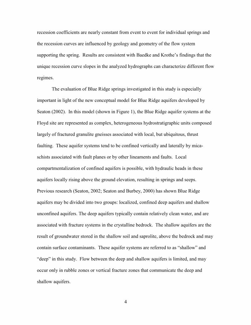
recession coefficients are nearly constant from event to event for individual springs and
the recession curves are influenced by geology and geometry of the flow system
supporting the spring. Results are consistent with Baedke and Krothe’s findings that the
unique recession curve slopes in the analyzed hydrographs can characterize different flow
regimes.
The evaluation of Blue Ridge springs investigated in this study is especially
important in light of the new conceptual model for Blue Ridge aquifers developed by
Seaton (2002). In this model (shown in Figure 1), the Blue Ridge aquifer systems at the
Floyd site are represented as complex, heterogeneous hydrostratigraphic units composed
largely of fractured granulite gneisses associated with local, but ubiquitous, thrust
faulting. These aquifer systems tend to be confined vertically and laterally by mica-
schists associated with fault planes or by other lineaments and faults. Local
compartmentalization of confined aquifers is possible, with hydraulic heads in these
aquifers locally rising above the ground elevation, resulting in springs and seeps.
Previous research (Seaton, 2002; Seaton and Burbey, 2000) has shown Blue Ridge
aquifers may be divided into two groups: localized, confined deep aquifers and shallow
unconfined aquifers. The deep aquifers typically contain relatively clean water, and are
associated with fracture systems in the crystalline bedrock. The shallow aquifers are the
result of groundwater stored in the shallow soil and saprolite, above the bedrock and may
contain surface contaminants. These aquifer systems are referred to as “shallow” and
“deep” in this study. Flow between the deep and shallow aquifers is limited, and may
occur only in rubble zones or vertical fracture zones that communicate the deep and
shallow aquifers.

5
The new model described by Seaton (2002) also proposes several different flow
pathways that may be important, especially with regard to groundwater recharge.
Distinct flow pathways in the Blue Ridge may include: flow through shallow saprolite
and regolith, flow through bedrock fractures, and flow along highly permeable zones
typically found above fault planes and referred to as shear zones or fault zones. Direct
connection of these flow pathways to spring outlets may be revealed by springflow
hydrographs. This study expands on the conceptual model proposed by Seaton (2002) in
an attempt to characterized the flow path ways associated with the complex aquifer
systems described in the Blue Ridge.

6
Figure 1 - New Blue Ridge Conceptual Model Proposed by Seaton (2002).
Fault plane
10’s of meters
100’s of meters
7
Objectives of this Investigation
The objective of this investigation is to correlate spring discharge with different
types of groundwater flow systems supplying water to the springhead at two sites in
Floyd and Grayson counties, Virginia. The Floyd County site is used to refine the
springflow hydrograph analysis technique and the Grayson County site is used to test the
method during one season of fieldwork. A combination of hydrophysical and
hydrochemical analyses with surface geophysics is used to ascertain the flow regimes that
influence the nature and character of Blue Ridge springs. A new device capable of
measurement of low discharge associated with the springs in each of these locations was
also developed as part of this study. If the springflow hydrograph technique proves valid,
it can be used to assess spring discharge sustainability and water, which are vitally
important when springs are used as potable water sources and sustainable yields are
necessary.
Geology, Physiography, and Geomorphology
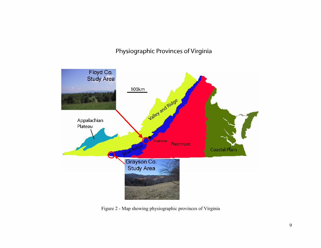
The locations of the field sites discussed in this investigation are shown in Figure
2. The Floyd and Grayson County sites are located on the Western edge of the Blue
Ridge Physiographic Province in Southwest Virginia.
The Blue Ridge Physiographic Province is an elongated band of exceptionally
complex geology stretching from central Pennsylvania to Georgia (Dietrich, 1959).
Composed of complexly faulted, fractured, and metamorphosed rocks, it is amongst the
most geologically and hydrogeologically complex area in the eastern United States. The
Blue Ridge is generally divided into two sections: a narrower, northern section extending
from the area north of Roanoke, VA, and a nearly 70 mile wide band south of Roanoke,

8
extending into North Carolina and Georgia (Clark et al., 1989). The field sites are
located in the southern section of the Blue Ridge.
9
Figure 2 - Map showing physiographic provinces of Virginia

10
The Northern Blue Ridge is typically a single ridge, surrounded by smaller
outlying isolated mountains. Some peaks in the Northern Blue Ridge exceed 1200 m,
and most of the drainages flow east to the Atlantic Ocean. The Southern Blue Ridge,
morphologically distinct from the Northern Blue Ridge, is typified by higher elevations,
multiple ridges, a large escarpment to the east, and drainage that flows west to the Gulf of
Mexico (Thornbury, 1965).
Geology and stratigraphy of the Blue Ridge are poorly documented in the area
between Roanoke and the North Carolina border. Geologic maps are sparse to non-
existent; state level mapping efforts are ongoing, but are still quite limited in extent.
Floyd County Field Site Description
The first field site location (hereafter referred to as the Floyd County site) is
located in southwest Virginia along Virginia route 810, 6 km west of Check, VA and 30
km south of Roanoke, VA. The field site is situated on the eastern rainwater divide,
which is an imaginary dividing line that separates overland flow so that rainfall on the
west side of the line flows into the Gulf of Mexico and rainfall on the east side of the line
flows into the Atlantic Ocean. The site is located in the Check quadrangle, near the
western edge of the Blue Ridge Physiographic Province.
Several different names have been given to the geologic formations underlying
Floyd County, the most recent and accepted being the Ashe Formation suggested by
Rankin (1970). The Ashe Formation consists of mica-schists, gneiss, and granites all of
metamorphic or igneous origin (Rankin, 1970; Seaton, 2001). Numerous overprinted
tectonic episodes have resulted in the fractured, faulted and metamorphosed geology
exposed at the field sites (Seaton, 2001).

11
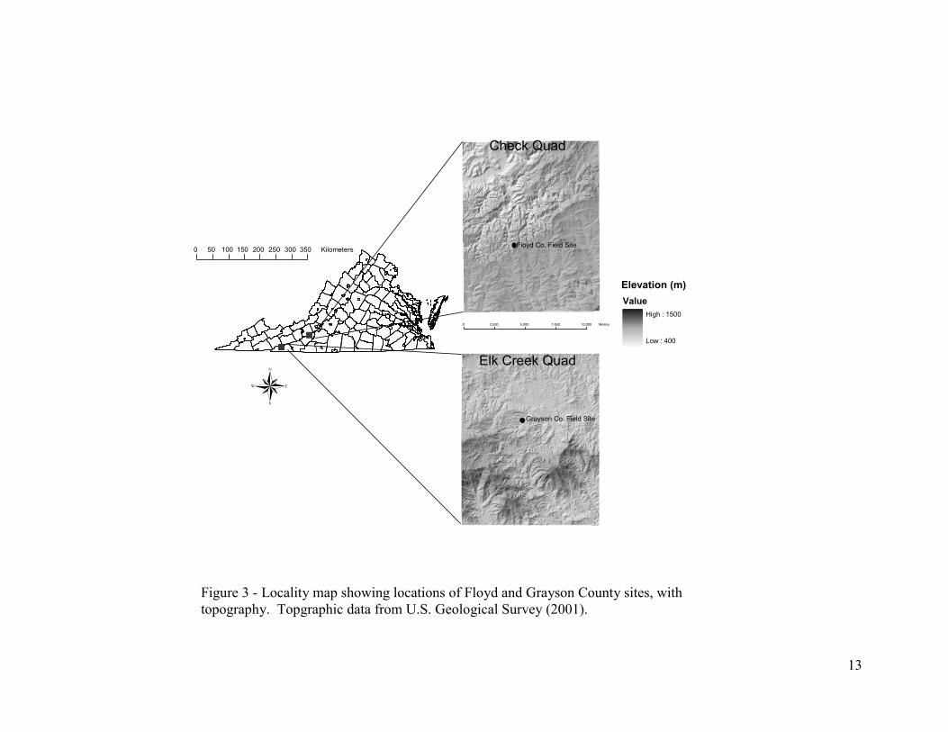
Topography in Floyd County is highly variable, ranging from relatively flat to
rolling lowlands around the western county border near Montgomery County to high
plateaus in the central portion of the county (Figure 3). The Blue Ridge Escarpment
defines the eastern boundary of Floyd County. The Blue Ridge Escarpment is
represented by an abrupt change in topography that is defined by the transition from the
Blue Ridge Province to the Piedmont Physiographic Province (Dietrich, 1959).
The average elevation in the Check quadrangle is 750.2 m, the minimum is 444.4
m and the maximum is 984.4 m occurring at an unnamed mountaintop in the northeast
corner of the quadrangle. A map showing the topography in the vicinity of this field site
is shown in Figure 3. Slopes in the Check quadrangle range from 0° near the South Fork
of the Roanoke River to a maximum of 58° in the more rugged portion located along the
Northwestern edge of the quad. The Floyd County site is characterized by fractured and
layered granulite gneiss bedrock typical of the Ashe Formation (Virginia Division of
Mineral Resources, 1993). Granulite gneiss typically has a very low hydraulic
conductivity (nearly impermeable). Local and regional faulting and fracturing have
created zones with high hydraulic conductivities within gneiss units. The permeable
granulite gneiss units are separated into individual hydrostratigraphic units by confining
units defined by mylonitic schists or unfractured gneiss (Seaton and Burbey, 2000).
Grayson County Field Site Description
The Grayson County site, located in Southwest Virginia along Virginia route 665
2.5 km southwest of Elk Creek, and 9.2 km northwest of Independence, is shown
topographically in Figure 3. The site is located in the Elk Creek quadrangle, near the
western edge of the Blue Ridge Physiographic province. The average elevation on the
Elk Creek Quadrangle is 928.0m, the minimum elevation is 741.4m and the maximum is
12
1403.0m occurring at Buck Mountain. Slopes in the Elk Creek Quad range from 0° in
the north central part of the quad to 54° near the mountains and more rugged terrain in
the southern part of the quad (Figure 3).
The Grayson County site is underlain by a biotite augen gneiss and represents part
of the Elk Park Plutonic Group which has previously been described as the Grayson
Gneiss (Popek, 1974). The Elk Park Plutonic Group outcrops west of the longitudinally
extensive Ashe Formation. While lithologically distinct from the Ashe Formation, the
Elk Park Plutonic Group contains many of the same overprinted tectonic events, resulting
in rocks that are faulted, and fractured similarly to the rocks at the Floyd County site.
13
0 50 100 150 200 250 300 350 Kilometers
0 2,500 5,000 7,500 10,000 Meters
Check Quad
Elk Creek Quad
Elevation (m)Value
High : 1500
Low : 400
Floyd Co. Field Site
Grayson Co. Field Site
"
®
"
Figure 3 - Locality map showing locations of Floyd and Grayson County sites, with topography. Topgraphic data from U.S. Geological Survey (2001).

14
Climate
Climate in Virginia is controlled primarily by distance from the Atlantic Ocean
and secondarily by topography (Crockett, 1971). The state is divided into three
topographic regions: Coastal Plain, Piedmont, and Western Mountain. Both field sites
mentioned in this study fall into the Western Mountain region. The Western Mountain
region is significantly cooler than locations in the Piedmont and Coastal Plain. Rainfall
is also influenced by proximity to the ocean and topography. Most significant rainfall
occurs on the southeastern and southwestern parts of the state with lesser amounts of rain
in the mountainous regions because of rainfall ‘blocking’ provided by the mountains
(Crockett, 1971). Annual rainfall for Virginia is dependent on the topographic region and
ranges from 36 to 52 inches. Long-term annual precipitation averages reported in 1985
for the two study areas in Floyd and Grayson counties are approximately 44 inches per
year (Moody et al., 1986). Rainfall is evenly distributed month-to-month throughout the
entire year, without significant wet or dry seasons. However, excessive rainfall
occasionally occurs during the fall months as infrequent hurricanes and tropical storms
pass over or near the state. The past four years (1998-2002) have been marked by
significant rainfall deficit with substantial departures from normal rainfall amounts.
Occasional droughts on the order of months are common in Virginia’s rainfall record,
however most are short lived and typically do not result in significant declines in aquifer
water levels. Longer-term droughts, on the order of several years, occur periodically and
may result in decline of aquifer water levels (Crockett, 1971).
15
Hydrogeology
Previous Work
Characterization of Blue Ridge hydrogeologic resources has not been a focus of
research in the past. Other studies in similar fractured rock aquifers have focused on
characterization of individual fractures and fracture geometry (Johnson, 1999; Karasaki
et al., 2000), but do not focus on flow pathways and aquifer characterization as a
complete unit. Recent water shortages and drought conditions have encouraged new
research into water sources and resource availability in the hydrogeologically complex
Blue Ridge and Piedmont regions (e.g., Seaton and Burbey, 2002). LeGrand’s USGS
circular (1967) is one of the first comprehensive synopses of groundwater systems in the
Blue Ridge. LeGrand mentions low-flow springs that vary little in yield, even during
prolonged dry spells. More recently, Seaton and Burbey (2000) have investigated water
resources in the Blue Ridge using numerous geophysical techniques, including surface
electrical resistivity and borehole logging. Seaton (2002) describes a new model of Blue
Ridge aquifer systems where clayey-schist layers confine hydrogeologic units and
recharge may occur along very permeable zones above fault planes. Long-term research
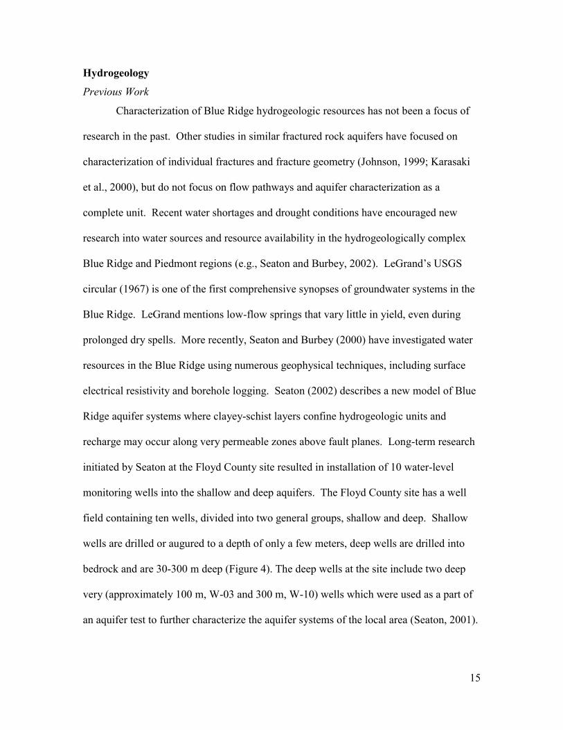
initiated by Seaton at the Floyd County site resulted in installation of 10 water-level
monitoring wells into the shallow and deep aquifers. The Floyd County site has a well
field containing ten wells, divided into two general groups, shallow and deep. Shallow
wells are drilled or augured to a depth of only a few meters, deep wells are drilled into
bedrock and are 30-300 m deep (Figure 4). The deep wells at the site include two deep
very (approximately 100 m, W-03 and 300 m, W-10) wells which were used as a part of
an aquifer test to further characterize the aquifer systems of the local area (Seaton, 2001).
16
"#
"#
#
#
"
"
"#
#P-01
W-08 W-07
W-10
W-03
W-05
W-04
W-01
W-02
W-06 W-09
SP-01
570732
570732
570932
570932
571132
571132
4099
942
4099
942
4100
142
4100
142
4100
342
4100
342
®Legend
Roads
Topography
Point Type" Deep Well
# Shallow Well/Piezometer
Spring
2800ft
2800ft
2700ft
0 50 10025 Meters
Figure 4 - Diagram showing well, piezometer and spring locations at Floyd county site.
17
Evidence of Multiple Flow Regimes
Many different tools can be used to characterize aquifer systems and flow paths.
Chlorofluorocarbons (CFC’s) can be used to date groundwater and can thus be used to
provide evidence of groundwater mixing. Geophysical well logs provide evidence of
fractures through interpretation of resistivity logs, and flow between fracture sets through
interpretation of borehole flowmeter data. Basic anion-cation water chemistry provides
evidence of groundwater mixing through concentration and dilution of specific anions
and cations. Surface electrical resistivity data results the yield information on the
geometry of the shallow subsurface; including fracture zones and possible aquifers. A
variety of tools were used by Seaton (2002) to characterize the hydrogeology of the Floyd
County site and suggest multiple flow regimes within the shallow and deep aquifers as
discussed below.
CFC Data
CFC age dating is a relatively common method used to obtain groundwater ages
of relatively young water (<60 years) by providing an approximate date since the
occurrence of groundwater recharge. CFC ages are dependent upon atmospheric
concentrations of CFC gases, their associated partial pressures, and recharge temperature.
The recharge temperature is typically quite stable because recharge takes place in the soil
where temperature fluctuations are minimized. Multiple CFC’s, such as CFC-11, CFC-
12, and CFC-113, are typically measured in each water sample to corroborate results and
provide a check against sample contamination by modern atmospheric air (Kozar et al.,
2000). Several wells at the Floyd County site were sampled for CFC’s, tritium/helium,
and SF6 (sulfur hexafluoride) as part of a regional groundwater age-dating study
18
performed by the U.S. Geological Survey in 1999. Results are described in detail in
Seaton (2002).
The CFC data collected by the U.S. Geological Survey yield evidence of two
distinct ages of water at the Floyd County site. The water is divided into two groups:
young, which has been in contact with the atmosphere within the past thirty years; and
old which has been isolated from the atmosphere for approximately thirty years or more.
Interpretation of the estimated dates obtained from the CFC data indicates that the
groundwater is 70-75% 60-year-old water mixed with 25-30% modern (<30 years old)
water. However, the data do not yield any information about the flow pathways or
mechanisms that may be allowing modern water to infiltrate and mix with the water in
the deeper, confined system.
Well Log Data
Geophysical well logging is a well-known technique for characterizing the
formation and formation fluids intersecting a borehole. Detailed geophysical well
logging was performed at the Floyd County site by Seaton (2002). Well logs for gamma
ray, spontaneous potential (SP), resistivity, caliper, fluid resistivity, temperature, and
heat-pulse flow meter were collected at each of the ten wells and at discrete depth
intervals. Geophysical logs, when interpreted together, can yield a host of information
about the subsurface including: probable lithologies, stagnant and flowing fracture zones,
saturated and unsaturated zones, and confining units. The heatpulse flow meter data
show distinct, flowing fracture zones associated with intensely fractured granulites, above
fault planes. Resistivity, gamma ray, and caliper logs show mica-schist aquitards
(confining units), and similar data from multiple wells scattered over the entire field area
suggest vertical fracture zones that communicate and allow flow between the deeper

19
aquifer system and shallower aquifer system. The same combined well-log data also
indicate changes in regolith and saprolite thickness associated with structural features that
may allow recharge to occur more readily in certain areas of the field site near fault
subcrops and associated highly permeable, fractured granulite zones (Seaton, 2002).
Chemistry
Water chemistry, analyzed as mean equivalent cations and anions, can indicate
relative water residence times. The longer groundwater is in contact with rock surfaces,
the higher the concentration of mean equivalent cations and anions. Other water
chemistry data, such as nitrate and phosphate concentrations, can indicate inputs of
nutrients from surface sources including fertilizers or septic drain fields and may act as
conservative or non-conservative tracers for tracking of groundwater. Seaton (2002)
describes the concentrations of cations and anions in wells completed in deep aquifers,
which indicates that concentrations are approximately double of those for wells
completed in the shallow aquifer system.
In this study, water samples were collected, filtered with a .45µm nylon filter and
analyzed for major anions at each spring and from wells in the vicinity of the springs at
both field sites. Initial water quality sampling (Summer 2001) consisted of analysis for
only nitrate and phosphate concentrations using a Hach DR/890 colorimeter. Later
(2002) water quality sampling consisted of an analysis for major anions (Br, Cl,
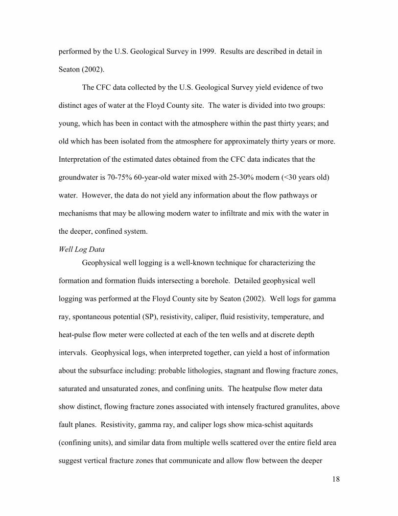
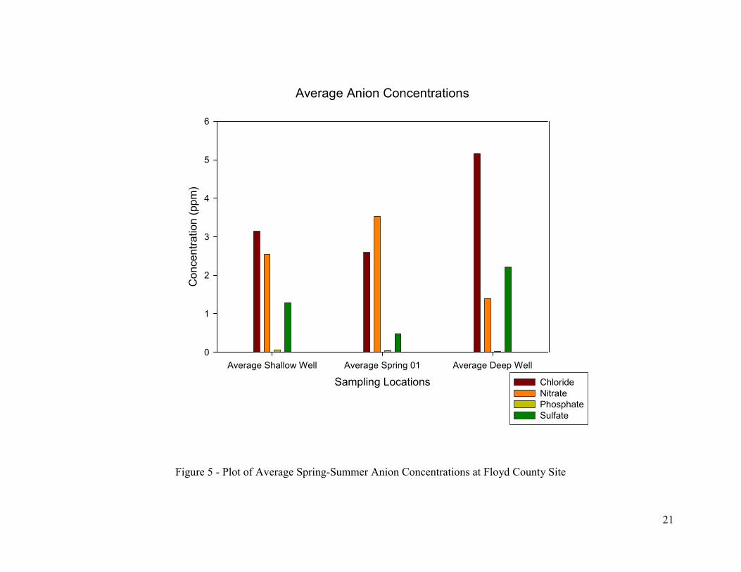
NO3,PO4, SO4) using ion chromatography. Figure 5 shows average anion concentrations
from groundwater and spring samples collected at the Floyd County site. Seaton (2002)
describes two distinct nitrate concentrations at the field area, which are comparable to the
values reported in this study (Figure 5). Deep wells have lower nitrate concentrations
while shallow wells have nitrate concentrations on the order of 1-3 parts per million. The
20
data shown in Figure 5 reflect a trend of lower nitrate concentrations in deeper wells and
higher concentrations in shallow wells. Concentrations of chloride and sulfate show the
opposite relationship with higher levels in the deep wells and lower levels in the shallow
wells. Phosphate concentrations in all samples were near or below detection limits for
the methods used. Concentrations of ions in water sampled from the spring, presented in
Figure 5, reflect a shallow source of water with higher concentration of nitrate and lower
concentrations of sulfate and chloride. These results suggest water at the spring outlet is
primarily sourced from the shallow aquifer. The next section, Spring Observations,
provides evidence to the contrary.
21
Average Anion Concentrations
Sampling LocationsAverage Shallow Well Average Spring 01 Average Deep Well
Con
cent
ratio
n (p
pm)
0
1
2
3
4
5
6
ChlorideNitratePhosphateSulfate
Figure 5 - Plot of Average Spring-Summer Anion Concentrations at Floyd County Site

22
Spring Observations
The CFC, geophysical well logs, and water chemistry data provide evidence of
multiple flow paths to the springhead at the Floyd site. The evidence of multiple flow
paths is corroborated by conversations with residents of the area who have used local
springs as sources of water for many years. Most residents have noted that some springs
go dry from year to year while others consistently discharge water at a constant rate for
years, or even decades. Some residents have noted that although springs may ‘cloud up’
with large amounts of sediment after rain events, the same springs discharge even during
drought conditions. The author also observed this phenomenon. Sediment is believed to
come from the shallow zone and is another indicator of a possible complex inter-aquifer
flow. Springs discharging perennially without significant variation in discharge, despite
long-term drought, suggest that they are at least partially connected to a deep flow path
with a more distant source of recharge and having long residence times. The
combination of both observations at a single spring outlet suggests a mixed deep and
shallow source.
Spring Discharge Measurements and Their Correlation to Rain Events
The springflow hydrograph analysis method of aquifer characterization requires a
record of spring discharge over time (a hydrograph) and a record of rain events for
correlation of discharge peaks and lag times. The period of discharge monitoring
required to adequately characterize a spring and the associated flow paths depends
entirely on rainfall. Widely separated rainfall events with easily correlated peaks give the
best results. Closely spaced rainfall events that result in complex overlapping peaks

23
where the spring discharge does not return to baseflow after each rainfall event provide
little help for analyzing hydrographs. However, good (easily interpreted) analysis results
can be obtained for hydrographs with widely separated rainfall events over a monitoring
period of weeks to months.
To measure precipitation, both field sites were each instrumented with data
loggers connected to tipping bucket rain gauges capable of measuring individual rain
events as small as 0.01 inches. Spring discharge is typically measured with a flume or
weir and a pressure transducer that records variations in water levels through the flume or
weir as discharge volumes increase or decrease. This method was not deemed feasible at
either field site because of low discharges associated with springs at each of the sites.
Discharges from springs at all field sites are typically below the lowest flow calibration
for flumes and weirs currently on the market. Development of a new system for
measurement of spring discharge was determined to be necessary to accurately monitor
the low discharge of the springs at each field site.
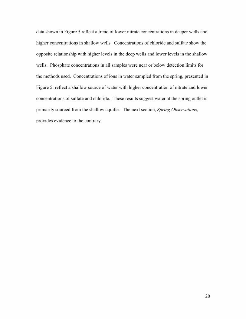
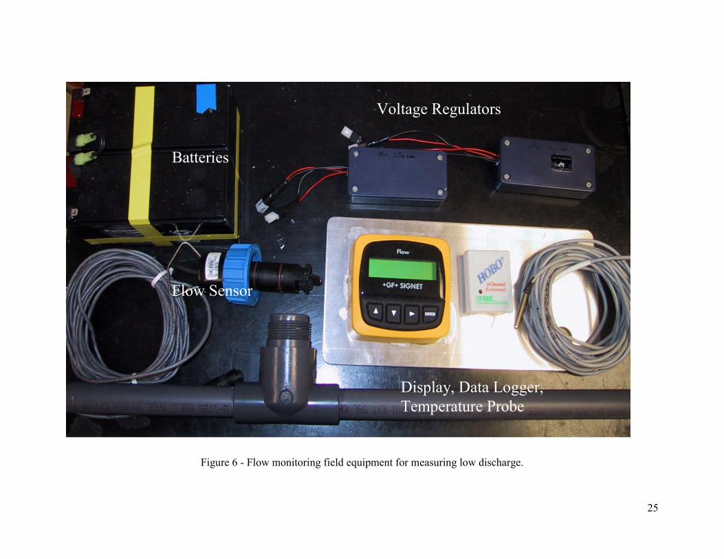
A new self-powered system (Low Flow Recording System, LoFRS) was designed
and built for use at the Floyd and Grayson sites. The system measures flow using off-
the-shelf manufacturing process control equipment including: a paddlewheel flow sensor,
a proprietary flow transmitter that converts the output of the flow sensor into a current
loop signal, and a data logger to record measurements made by the discharge-
measurement system. This system is shown in Figure 6 and diagrammed in Appendix I.
Solar cells and small voltage regulators provide controlled voltages and currents
for charging the batteries and powering the discharge-measurement system. The data-
logging system also records water temperature using a small stainless steel encased

24
thermistor probe. Multiple channels are available on the logging system, allowing for
future expansion of additional probes such as dissolved oxygen, pH, fluid conductivity,
and fluid pressure. Field calibration of the flow system was not necessary, the
manufacturer supplies a lab-calibrated tee fitting with the flow measurement system that
allows for conversion of fluid velocity to flow rate. The calibration is valid for fluid
velocities in which the probe is capable of producing an output.
A table containing dates of the spring monitoring periods is shown below (Table
2). Field equipment at the Floyd County site experienced substantial downtime due to
damage caused by grazing livestock in the field area. Field equipment could not be left
to record discharge in the colder months because freezing water would destroy the flow
sensor. The flow monitor requires springflow to be through a pipe to allow for
connection of the discharge sensor. Springs at the Grayson County site, GSP-04 and
GSP-05, are discussed later in the section titled Applications to Other Locations.
Spring Location Monitoring PeriodSP-01 Floyd County site 6/18/01-8/1/01, 6/28/02-8/1/02, & 9/22/02-10/5/02GSP-04 Grayson County site 5/22/02-6/11/02GSP-05 Grayson County site 6/11/02-11/11/02
Table 2 - Spring discharge monitoring periods
Several reference measurements of winter spring flow were recorded in the winter of
2001 and 2002 at SP-01. Winter discharge measurements were recorded with a gallon
jug and stopwatch. Typical winter discharge for spring SP-01 is approximately 3
gallons/minute.
25
Voltage Regulators
Batteries
Flow Sensor
Display, Data Logger, Temperature Probe
Figure 6 - Flow monitoring field equipment for measuring low discharge.
26
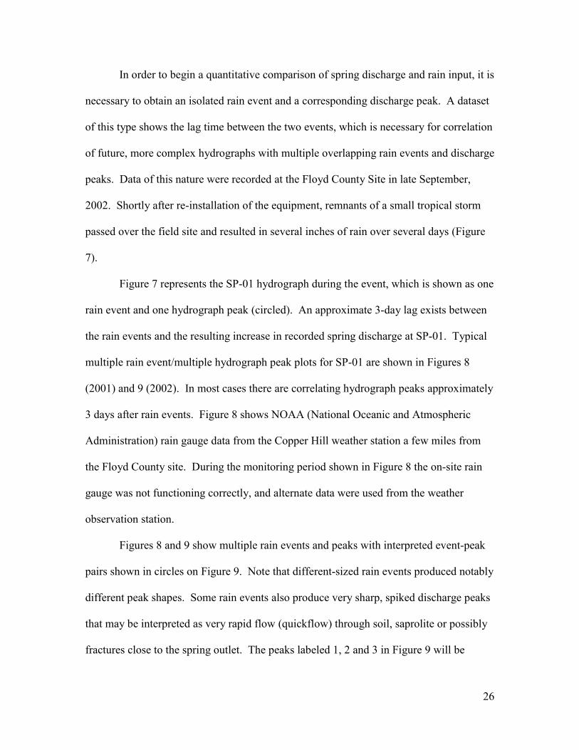
In order to begin a quantitative comparison of spring discharge and rain input, it is
necessary to obtain an isolated rain event and a corresponding discharge peak. A dataset
of this type shows the lag time between the two events, which is necessary for correlation
of future, more complex hydrographs with multiple overlapping rain events and discharge
peaks. Data of this nature were recorded at the Floyd County Site in late September,
2002. Shortly after re-installation of the equipment, remnants of a small tropical storm
passed over the field site and resulted in several inches of rain over several days (Figure
7).
Figure 7 represents the SP-01 hydrograph during the event, which is shown as one
rain event and one hydrograph peak (circled). An approximate 3-day lag exists between
the rain events and the resulting increase in recorded spring discharge at SP-01. Typical
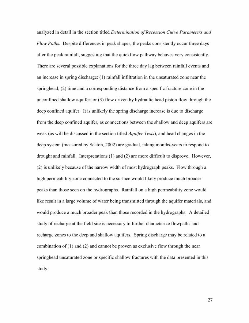
multiple rain event/multiple hydrograph peak plots for SP-01 are shown in Figures 8
(2001) and 9 (2002). In most cases there are correlating hydrograph peaks approximately
3 days after rain events. Figure 8 shows NOAA (National Oceanic and Atmospheric
Administration) rain gauge data from the Copper Hill weather station a few miles from
the Floyd County site. During the monitoring period shown in Figure 8 the on-site rain
gauge was not functioning correctly, and alternate data were used from the weather
observation station.
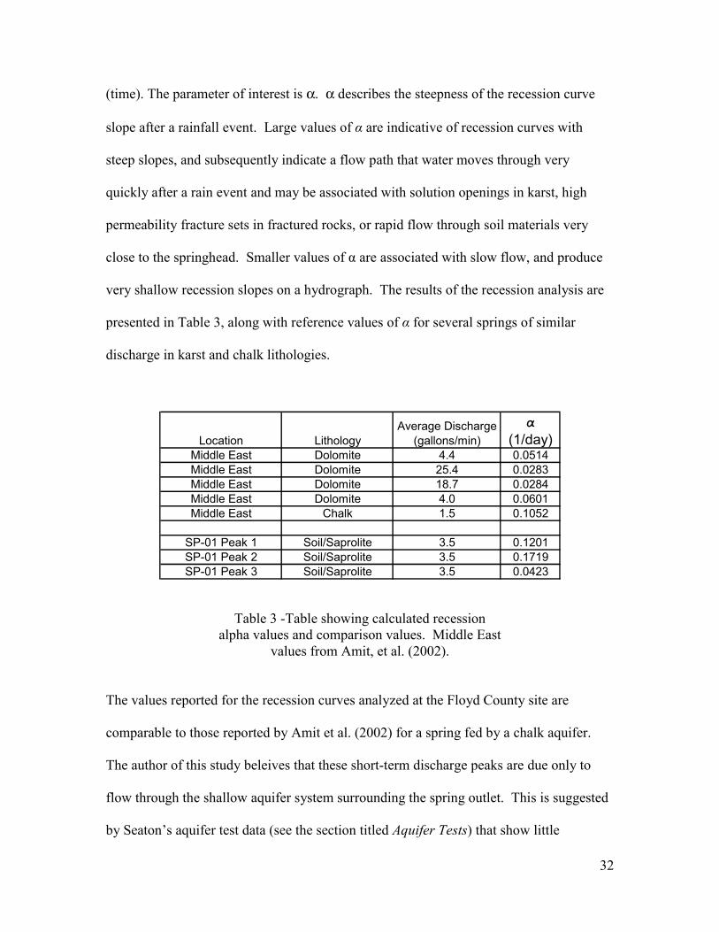
Figures 8 and 9 show multiple rain events and peaks with interpreted event-peak
pairs shown in circles on Figure 9. Note that different-sized rain events produced notably
different peak shapes. Some rain events also produce very sharp, spiked discharge peaks
that may be interpreted as very rapid flow (quickflow) through soil, saprolite or possibly
fractures close to the spring outlet. The peaks labeled 1, 2 and 3 in Figure 9 will be
27
analyzed in detail in the section titled Determination of Recession Curve Parameters and
Flow Paths. Despite differences in peak shapes, the peaks consistently occur three days
after the peak rainfall, suggesting that the quickflow pathway behaves very consistently.
There are several possible explanations for the three day lag between rainfall events and
an increase in spring discharge: (1) rainfall infiltration in the unsaturated zone near the
springhead; (2) time and a corresponding distance from a specific fracture zone in the
unconfined shallow aquifer; or (3) flow driven by hydraulic head piston flow through the
deep confined aquifer. It is unlikely the spring discharge increase is due to discharge
from the deep confined aquifer, as connections between the shallow and deep aquifers are
weak (as will be discussed in the section titled Aquifer Tests), and head changes in the
deep system (measured by Seaton, 2002) are gradual, taking months-years to respond to
drought and rainfall. Interpretations (1) and (2) are more difficult to disprove. However,
(2) is unlikely because of the narrow width of most hydrograph peaks. Flow through a
high permeability zone connected to the surface would likely produce much broader
peaks than those seen on the hydrographs. Rainfall on a high permeability zone would
like result in a large volume of water being transmitted through the aquifer materials, and
would produce a much broader peak than those recorded in the hydrographs. A detailed
study of recharge at the field site is necessary to further characterize flowpaths and
recharge zones to the deep and shallow aquifers. Spring discharge may be related to a
combination of (1) and (2) and cannot be proven as exclusive flow through the near
springhead unsaturated zone or specific shallow fractures with the data presented in this
study.

28
Floyd Co. SP-012002 Monitoring
Single Event -Tropical Depression
Date9/20/2002 9/22/2002 9/24/2002 9/26/2002 9/28/2002 9/30/2002
Sprin
gflo
w (g
allo
ns p
er m
inut
e)
5.0
5.5
6.0
6.5
7.0
7.5
Rai
nfal
l (in
ches
)
0.0
0.2
0.4
0.6
0.8
1.0
SP-01Rain Gauge Data
Figure 7 - Plot of spring discharge and rain for an isolated rain event at the Floyd County site.

29
Floyd Co. SP-012001 Monitoring
Date6/18/2001 6/25/2001 7/2/2001 7/9/2001 7/16/2001 7/23/2001 7/30/2001
Rai
nfal
l (in
ches
)
0.0
0.5
1.0
1.5
2.0
2.5
Sprin
gflo
w (g
allo
ns p
er m
inut
e)
0
1
2
3
4
5
Rain Gauge Data
SP-01 Flow Rate
Figure 8 – Plot of spring discharge and rain at the Floyd County site. Rain data from NOAA (on-site rain gauge malfunctioned)
Sharp peak, characteristic of shallow, or rapid flow

30
Floyd Co. SP-012002 Monitoring
Date6/28/2002 7/2/2002 7/6/2002 7/10/2002 7/14/2002 7/18/2002 7/22/2002
Sprin
gflo
w (g
allo
ns p
er m
inut
e)
0
2
4
6
8
Rai
nfal
l (in
ches
)
0.0
0.1
0.2
0.3
0.4
0.5
SP-01 FlowrateRain Gauge Data
Figure 9 - Another typical multiple rain event, multiple hydrograph peak plot from the summer of 2002 at the Floyd County
12
3

31
Determination of Recession Curve Parameters and Flow Paths
One benefit of the springflow hydrograph method is its ability to reveal
quantitative data about the aquifer and/or flow path providing water to the spring outlet.
Analysis of recession curves can yield values for transmissivity or specific yield if
storativity and distance to groundwater divide are known apriori. In this investigation,
these aquifer parameters are not known. Analysis of the recession curve parameters is
thus limited to calculation of recession curve slope, which indicates the relative speed
that water drains from flow paths supplying the spring outlet. Steeper slopes are
correlated to rapid drainage of flow paths and higher hydraulic conductivities; shallower
slopes are correlated to slower drainage of flow paths and lower hydraulic conductivities.
Figure 8 (data from 2001) was not fit with recession curve slopes because of the very
closely spaced rain events, and the difficulty of interpreting rainfall/hydrograph peak
pairs. The difficulty in finding correlated peaks may be related to the offsite raingauge
data used for this time period. Rainfall at the Copper Hill weather station may not
accurately reflect the rainfall at the Floyd site only a few kilometers away. The three
peaks circled and labeled in Figure 9 (data from 2002) were analyzed to determine the
recession curve slopes. Each peak was isolated from the time series discharge data
shown in Figure 9 and an exponential decay curve in the form of the Boussinesq
Equation (2) was fit using SigmaPlot’s (2001) regression function in a method similar to
that applied by Amit et al (2002).
teQQ α−= 0 (2)
Where Q is the discharge at the end of the recession, Q0 is the discharge at the beginning
of the recession, α is the recession coefficient, and t is the duration of the recession
32
(time). The parameter of interest is α. α describes the steepness of the recession curve
slope after a rainfall event. Large values of α are indicative of recession curves with
steep slopes, and subsequently indicate a flow path that water moves through very
quickly after a rain event and may be associated with solution openings in karst, high
permeability fracture sets in fractured rocks, or rapid flow through soil materials very
close to the springhead. Smaller values of α are associated with slow flow, and produce
very shallow recession slopes on a hydrograph. The results of the recession analysis are
presented in Table 3, along with reference values of α for several springs of similar
discharge in karst and chalk lithologies.
Middle East Dolomite 4.4 0.0514Middle East Dolomite 25.4 0.0283Middle East Dolomite 18.7 0.0284Middle East Dolomite 4.0 0.0601Middle East Chalk 1.5 0.1052
SP-01 Peak 1 Soil/Saprolite 3.5 0.1201SP-01 Peak 2 Soil/Saprolite 3.5 0.1719SP-01 Peak 3 Soil/Saprolite 3.5 0.0423
LithologyAverage Discharge
(gallons/min)α
(1/day)Location
Table 3 -Table showing calculated recession alpha values and comparison values. Middle East
values from Amit, et al. (2002).
The values reported for the recession curves analyzed at the Floyd County site are
comparable to those reported by Amit et al. (2002) for a spring fed by a chalk aquifer.
The author of this study beleives that these short-term discharge peaks are due only to
flow through the shallow aquifer system surrounding the spring outlet. This is suggested
by Seaton’s aquifer test data (see the section titled Aquifer Tests) that show little

33
connection between the deep and shallow aquifers except near a zone of intense
fracturing located approximately 25 m upgradient from the spring. The short total
duration (magnitude and width) of discharge peaks, which can be correlated to source
areas, also suggests that the peaks are related to flow only through the shallow zone.
Sharp discharge peaks are typical of a small source area. If an assumption is made that
the area under a hydrograph peak is related to the total rainfall during an individual
rainfall event, the area of the location where the rainfall infiltrated can be calculated.
This calculation is performed by integrating the area under a hydrograph peak to obtain
the total discharge for a single rain event, then dividing the discharge volume by rainfall
depth to obtain an estimate of the area where the rainfall infiltrated. The amount of water
discharged from the spring outlet must be compensated for losses such as evaporation
and runoff and is multiplied by 150% (an approximation). Performing this analysis on
the spring at the Floyd site, for the single even isolated in Figure 7 yields a recharge area
of only a few hundred square feet. Peaks from flow through a deeper system, with a
larger recharge area would likely be much broader because of the likely larger volume of
water that would enter the aquifer from a larger recharge area. SP-01 Peak 3 shows a
different recession mode, approximately 1/3 of the slopes from peaks 1 and 2. This could
be due to the extended rainfall associated with the peak, and subsequent saturation and
slower flow along longer paths in the unsaturated zone. To use the recession method for
determination of deep aquifer parameters, a record of spring discharge during baseflow
conditions would be necessary. The spring at the Floyd site typically shows a baseflow
response only during extended droughts (months without rain) during the summer and
during the winter when precipitation (snow) evaporates before it can enter the shallow

34
aquifer. Such a record was not recorded because of concerns about freezing temperatures
and possible subsequent damage to the flow sensor.
Identification of specific flow paths requires additional information. The
hydrographs clearly reveal the influence of rapid flow through the shallow aquifer, but
provide less evidence of possible flow through the deeper fault zone aquifer. Electrical
resistivity was implemented to evaluate other possible flow paths, including those
through the deeper fault zone aquifer.
Resistivity Characterization of Geology and Hydrology
Electrical resistivity surveying is a geophysical technique used for investigation of
shallow anomalies such as changes in rock or moisture conditions (Seaton and Burbey,
2002). The technique consists of a numerous measurements of potential (voltage)
between two electrodes while a constant current is applied between two other electrodes.
The points at which the potential is measured and the current is applied are systematically
widened, resulting in deeper, longer current flow paths that sample more of the
subsurface. The electrodes are placed at known spacings (geometry shown in Appendix
II) and the current supplied is known, making calculation of apparent earth resistivity
quite simple using the following equation for the dipole-dipole array which was used for
this study (Sharma, 1997):
( )( )IVnnnaa
∆++⋅⋅⋅= 21πρ (1)
Where aρ is the calculated resistivity, a is the electrode spacing, n is an incremented
variable, ∆V is the potential difference measured, and I is the input current. The
measured potential and calculated resisitivities are the result of the interaction of the
supplied constant current and the electrical resistivity of the flow path along which the
35
electric current has traveled and incorporates all resistivity heterogeneities along the flow
path into the recorded measurement. It is necessary to invert the dataset to calculate a
resistivity model of the subsurface that incorporates the heterogeneities measured as the
current flows through the subsurface. Inversion of resistivity data is typically completed
with a non-linear inversion-modeling program, such as RES2DINV (Loke, 2002; Loke
and Barker, 1995).
Resistivity Techniques and Interpretation
Surface geophysical resistivity imaging was used for characterization of the
aquifer systems surrounding the springheads at both study sites. A Campus Geopulse 25
electrode system records 178 measurements using a dipole-dipole array (see Appendix
II). The dipole-dipole array provides the best compromise between depth and resolution
in the geologic medium present at both the Floyd and Grayson sites (Seaton and Burbey,
2002). The measurements taken by the geopulse unit are recorded together with
electrode spacing and are referred to as a resistivity line.
Transitions between typical Blue Ridge Province media (soil, saprolite, etc.)
affect the resistivity of the matrix material, and result in imageable resistivity changes.
Large resistivity transitions, on the scale of several orders of magnitude, occur in
saturated zones due to the significantly higher conductivity of water containing dissolved
ions. Similar transitions occur at the regolith bedrock interface where resistivity
increases, again by several orders of magnitude, at the transition between soil and solid
bedrock.
2-dimensional resistivity models computed for each resistivity line were
optimized for minimum root mean square (RMS) error between the observed data and
calculated data obtained from forward modeling. In most cases RMS error values of less
36
than 10% exist between observed resistivity sections and earth resistivity calculated from
the final models. The most important inversion modeling parameter for model
optimization is the “robust constraint” option provided in RES2DINV. The traditional
least-squares inversion method attempts to minimize the error by minimizing the squared
difference of measured and calculated data, but is quite susceptible to “noise” in the field
dataset. The “robust constraint” attempts to minimize the absolute difference (rather than
the squared difference of the least squares method) to optimize the model. Consequently,
the “robust constraint” is less susceptible to noise spikes or shallow electrode-related
spikes that are prevalent in Blue Ridge resistivity data. The robust constraint results in
reduced model resolution because of the ‘blocky’, large model cells that result from the
use of the “robust constraint” (Loke, 2002). Electrical resistivity is ideal for use in the
Blue Ridge because of the large resistivity change between shallow soil, deeper
crystalline bedrock, fractures, variably saturated soil and saprolite, and fault zones.
Misfits between the modeled and observed data remaining after processing may be
remnants of small heterogeneities in the shallow subsurface.
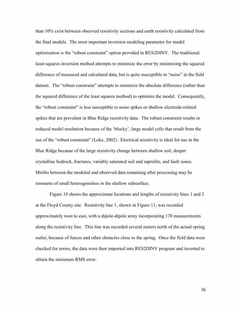
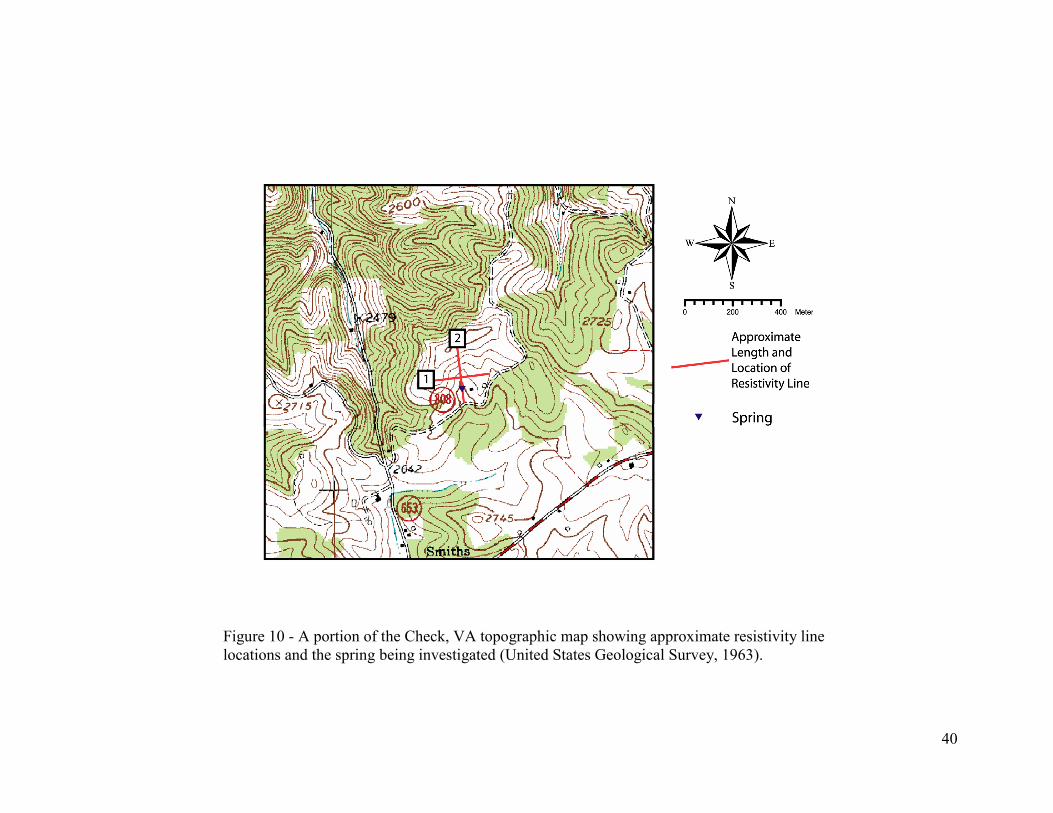
Figure 10 shows the approximate locations and lengths of resistivity lines 1 and 2
at the Floyd County site. Resistivity line 1, shown in Figure 11, was recorded
approximately west to east, with a dipole-dipole array incorporating 178 measurements
along the resistivity line. This line was recorded several meters north of the actual spring
outlet, because of fences and other obstacles close to the spring. Once the field data were
checked for errors, the data were then imported into RES2DINV program and inverted to
obtain the minimum RMS error.

37
Figures 11 and 12 each show several anomalies that are of interest in this study.
Figure 11 has a distinct high resistivity anomaly near the left center portion of the section.
This anomaly is modeled as having a constant resistivity, and is homogenous. The right
side of the section shows a lower resistivity anomaly that is roughly ‘U’ shaped
containing a roughly circular low resistivity body and bounded by the high resistivity,
homogenous anomaly on the left side of the survey and a few model cells shown as
higher resistivity on the right side. Two elliptical high resistivity anomalies are shown in
the upper left portion of the model with the rest of the shallow portion of the model
having a relatively low, variable resistivity. Figure 12 is a crossline of Figure 11,
crossing Figure 11 at approximately 120m from the left end. Figure 12 shows a
homogenous, roughly elliptical body near the center of the model that is bounded on all
sides by lower resisitivities. The zone below this large, homogenous body is modeled as
having a lower resistivity similar to that of the shallow (first few meters) of the model
above the homogenous body. A low resistivity, homogenous body is located just left of
the elliptical, high resistivity body. The remainder of the shallow portion of the model is
modeled as having relatively low, variable resistivity.
Interpretation of the Figures 11 and 12 is based on outcrops, water-level
observations collected by the author and by Seaton (2002), and based on fracture zones
previously documented by Seaton and Burbey (2002). Generally, decreases in resistivity
are correlated with increases in soil/rock saturation. The addition of water to the soil or
bedrock increases the conductivity. Bedrock in the area is crystalline, and when intact
(containing no fractures) has a very high resistivity. This is confirmed by resistivity well
logs, collected by Seaton (2002). Fractures and fracture zones in bedrock generally result
38
in lower resisitivities than bedrock alone because of water or air that are present in the
fracture or fracture zone. Other features, such as quartz veins and boulders, are easily
identified in outcrop. The resistivity data are also interpreted in the context of Seaton’s
(2002) model (discussed below). Using multiple data allow the author to make precise
interpretations of anomalies appearing in the modeled electrical resistivity data.
Figures 11 and 12 show the anomalies marked with probable interpretations,
based on the field evidence mentioned above. Possible flow pathways are marked, and
will be discussed later.
Numerous surface electrical resistivity surveys have been performed at the Floyd
site by Seaton (2002; Seaton and Burbey, 2002) and by the author of this study. The
analyses of the surveys conducted by Seaton and Burbey (2002) were instrumental in the
development of the new Blue Ridge conceptual model. The model, presented in Figure 1
(Seaton, 2002), is largely dependent on electrical resistivity imaging of fracture zones.
Fracture zones are not always imaged as low resistivity anomalies because of limited
resolution of electrical resistivity surveys. Minute fractures are well below the size of
features that can be characterized by resistivity imaging. However, large fractures zones
with intensely fractured rocks are imageable because of large volume of rock affected by
the fracturing.
Seaton and Burbey (2002) present evidence of a high-permeability horizontal
fracture zone, represented by intensely fractured rocks and their subsequent lower
resistivity, these high permeability zones above the fault plane are referred to here as a
fault zone or shear zone. Other dispersed fracture zones are scattered throughout the field
site (see Seaton, 2002). The fracture zone is believed to represent the deep aquifer

39
system at the site. The resistivity data interpreted by Seaton indicate that these fracture
zones may be saturated, moist, or dry, depending on climate conditions and it is probable
that they may become saturated and transmit water during rainfall events.
40
Figure 10 - A portion of the Check, VA topographic map showing approximate resistivity line locations and the spring being investigated (United States Geological Survey, 1963).
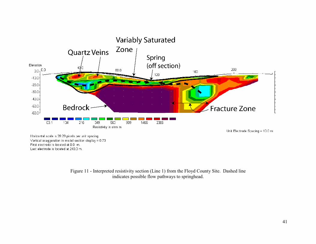
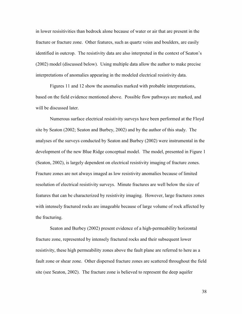
41
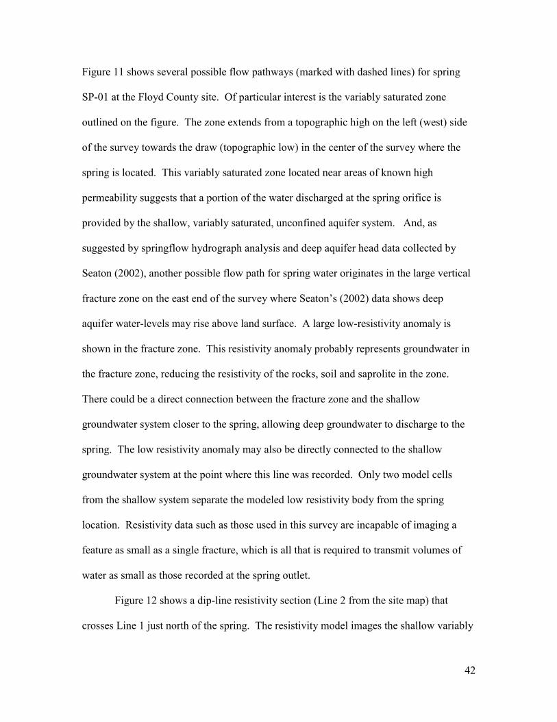
Figure 11 - Interpreted resistivity section (Line 1) from the Floyd County Site. Dashed line indicates possible flow pathways to springhead.
42
Figure 11 shows several possible flow pathways (marked with dashed lines) for spring
SP-01 at the Floyd County site. Of particular interest is the variably saturated zone
outlined on the figure. The zone extends from a topographic high on the left (west) side
of the survey towards the draw (topographic low) in the center of the survey where the
spring is located. This variably saturated zone located near areas of known high
permeability suggests that a portion of the water discharged at the spring orifice is
provided by the shallow, variably saturated, unconfined aquifer system. And, as
suggested by springflow hydrograph analysis and deep aquifer head data collected by
Seaton (2002), another possible flow path for spring water originates in the large vertical
fracture zone on the east end of the survey where Seaton’s (2002) data shows deep
aquifer water-levels may rise above land surface. A large low-resistivity anomaly is
shown in the fracture zone. This resistivity anomaly probably represents groundwater in
the fracture zone, reducing the resistivity of the rocks, soil and saprolite in the zone.
There could be a direct connection between the fracture zone and the shallow
groundwater system closer to the spring, allowing deep groundwater to discharge to the
spring. The low resistivity anomaly may also be directly connected to the shallow
groundwater system at the point where this line was recorded. Only two model cells
from the shallow system separate the modeled low resistivity body from the spring
location. Resistivity data such as those used in this survey are incapable of imaging a
feature as small as a single fracture, which is all that is required to transmit volumes of
water as small as those recorded at the spring outlet.
Figure 12 shows a dip-line resistivity section (Line 2 from the site map) that
crosses Line 1 just north of the spring. The resistivity model images the shallow variably
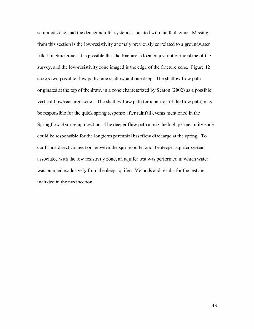
43
saturated zone, and the deeper aquifer system associated with the fault zone. Missing
from this section is the low-resistivity anomaly previously correlated to a groundwater
filled fracture zone. It is possible that the fracture is located just out of the plane of the
survey, and the low-resistivity zone imaged is the edge of the fracture zone. Figure 12
shows two possible flow paths, one shallow and one deep. The shallow flow path
originates at the top of the draw, in a zone characterized by Seaton (2002) as a possible
vertical flow/recharge zone . The shallow flow path (or a portion of the flow path) may
be responsible for the quick spring response after rainfall events mentioned in the
Springflow Hydrograph section. The deeper flow path along the high permeability zone
could be responsible for the longterm perennial baseflow discharge at the spring. To
confirm a direct connection between the spring outlet and the deeper aquifer system
associated with the low resistivity zone, an aquifer test was performed in which water
was pumped exclusively from the deep aquifer. Methods and results for the test are
included in the next section.

44
Figure 12 - Interpreted resistivity section (Line 2) from the Floyd County Site. Dashed line indicates possible flow pathways to springhead.
45
Aquifer Tests
A six-day aquifer test was performed by Seaton (2002) at the Floyd County site in
the spring of 2001. Water was withdrawn from deep well W-07 situated near the center
of the site to test for fracture connections between wells (Figure 4). The data from the
aquifer test show practically no connection between the shallow and deep aquifers.
Water level declines in the shallow system were negligible, suggesting no significant
flow pathways between the deep and shallow aquifers near the well being pumped.
Water-level declines in the well and deep aquifer occurred slowly (over a 6 day period)
during pumping with aquifer materials surrounding the well behaving much like an
extended well. Analysis of pumping and recovery data suggests that the deep wells are
connected by a network of highly transmissive fractures that convey water rapidly to the
pumping well, this network of fractures is described as the fault zone aquifer (Seaton,
2002). Interpretation of the data suggests water is flowing in the aquifers on two
different times scales. Flow within the deep aquifer is rapid because of the high
hydraulic conductivity of the fracture system that comprises the deep aquifer, and flow
between the shallow and deep aquifers is very slow because of the low hydraulic
conductivity of the confining units separating the two aquifers (Seaton, 2001).
In November of 2002 an additional aquifer test was performed at the Floyd
County site by the author of this study to determine a connection between the deep fault
zone aquifer and the spring SP-01. The test was designed to evaluate flow between the
deep aquifer and the spring outlet and complements the data collected in Seaton’s (2002)
aquifer test that characterized the flow between the shallow and deep aquifers. Deep well
W-03 (Figure 4) was packed off just above the producing fracture zone indicated by
Seaton (2002) to ensure only the deep aquifer was pumped and there was no connection

46
with the shallow aquifer. The discharge of SP-01 was monitored through the duration of
pumping and for several hours after pumping. W-03 was pumped at 2.5-3.0 gallons per
minute for 4 hours resulting in nearly 180 feet of drawdown measured in the pumped
well over approximately 3 hours. In addition to monitoring of the pumping well and
spring discharge rates during pumping, water samples were taken at half hour intervals
from the pumped well and from the spring in an attempt to characterize changes in water
chemistry during the pumping test. If the pre-aquifer test spring water is a mix of water
from the shallow and deep aquifers, and pumping W-03 reduces the head in the deep
aquifer so it no longer provides water to the spring outlet, the water chemistry during and
after the aquifer test will resemble the chemistry of the shallow aquifer sampled at P-01.
If the pre-aquifer test spring water is solely from the deep aquifer, the water chemistry
will no resemble the chemistry of the shallow aquifer during or after the test.
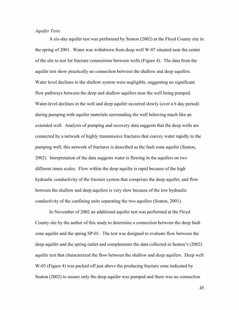
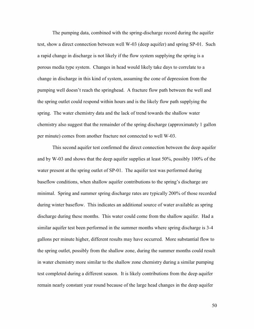
The results of the aquifer test are shown in Figure 13. This figure shows spring
discharge and pumping well discharge for the duration of the aquifer test. The results
show that spring discharge decreased by more than 50% as the well was pumped. The
spring responds almost instantly as pumping begins and the well is water level in the well
is lowered. The spring also recovers almost as quickly after pumping ends. This
suggests the well and spring are connected by a flow pathway with a very high hydraulic
conductivity (such as a fracture, or fracture network). Spring discharge was reduced by
approximately 2/3 after 3 hours of pumping. This suggests that a majority of the spring’s
discharge was from the deep aquifer pumped at well W-03. The remainder of the
discharge may come from another fracture or from the shallow zone.

47
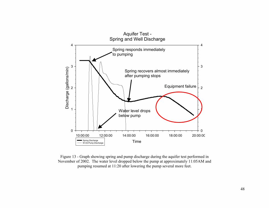
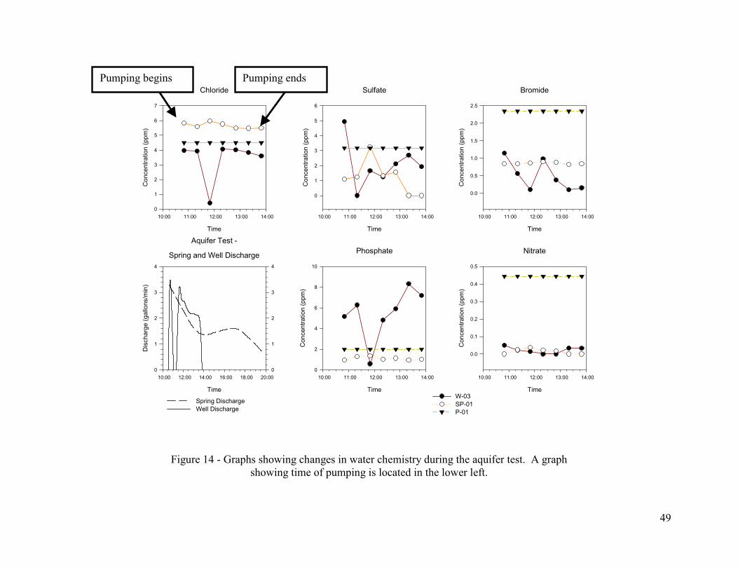
Figure 14 shows temporal changes in anion water chemistry from the samples
collected at half hour intervals during the pumping duration of the aquifer test.
Additional samples were collected from a piezometer (P-01) located beside W-03 for
comparison of water chemistry from the shallow and deep aquifers. The anomalous data
points in the chloride, phosphate and bromide plots (zero or near zero concentrations)
may be due to analysis error (incorrect peak picking by the chromatography software).
The anion chemistry from the spring does not trend towards the water chemistry of the
shallow zone (high nitrate content) sampled at P-01. This suggests the water discharged
from the spring outlet, even after significant pumping of W-03 may come from another
fracture, rather than the shallow aquifer.
48
Aquifer Test -Spring and Well Discharge
Time 10:00:00 12:00:00 14:00:00 16:00:00 18:00:00 20:00:00
Dis
char
ge (g
allo
ns/m
in)
0
1
2
3
4
0
1
2
3
4
Spring DischargeW-03-Pump DIscharge
Figure 13 - Graph showing spring and pump discharge during the aquifer test performed in November of 2002. The water level dropped below the pump at approximately 11:05AM and
pumping resumed at 11:20 after lowering the pump several more feet.
Water level drops below pump
Spring responds immediately to pumping
Spring recovers almost immediately after pumping stops
Equipment failure
49
Chloride
Time
10:00 11:00 12:00 13:00 14:00
Con
cent
ratio
n (p
pm)
0
1
2
3
4
5
6
7
Bromide
Time
10:00 11:00 12:00 13:00 14:00
Con
cent
ratio
n (p
pm)
0.0
0.5
1.0
1.5
2.0
2.5
Phosphate
Time
10:00 11:00 12:00 13:00 14:00
Con
cent
ratio
n (p
pm)
0
2
4
6
8
10
Sulfate
Time
10:00 11:00 12:00 13:00 14:00
Con
cent
ratio
n (p
pm)
0
1
2
3
4
5
6
Aquifer Test -
Spring and Well Discharge
Time
10:00 12:00 14:00 16:00 18:00 20:00
Dis
char
ge (g
allo
ns/m
in)
0
1
2
3
4
0
1
2
3
4
Spring DischargeWell Discharge
Nitrate
Time
10:00 11:00 12:00 13:00 14:00
Con
cent
ratio
n (p
pm)
0.0
0.1
0.2
0.3
0.4
0.5
W-03SP-01P-01
Figure 14 - Graphs showing changes in water chemistry during the aquifer test. A graph showing time of pumping is located in the lower left.
Pumping begins Pumping ends
50
The pumping data, combined with the spring-discharge record during the aquifer
test, show a direct connection between well W-03 (deep aquifer) and spring SP-01. Such
a rapid change in discharge is not likely if the flow system supplying the spring is a
porous media type system. Changes in head would likely take days to correlate to a
change in discharge in this kind of system, assuming the cone of depression from the
pumping well doesn’t reach the springhead. A fracture flow path between the well and
the spring outlet could respond within hours and is the likely flow path supplying the
spring. The water chemistry data and the lack of trend towards the shallow water
chemistry also suggest that the remainder of the spring discharge (approximately 1 gallon
per minute) comes from another fracture not connected to well W-03.
This second aquifer test confirmed the direct connection between the deep aquifer
and by W-03 and shows that the deep aquifer supplies at least 50%, possibly 100% of the
water present at the spring outlet of SP-01. The aquifer test was performed during
baseflow conditions, when shallow aquifer contributions to the spring’s discharge are
minimal. Spring and summer spring discharge rates are typically 200% of those recorded
during winter baseflow. This indicates an additional source of water available as spring
discharge during these months. This water could come from the shallow aquifer. Had a
similar aquifer test been performed in the summer months where spring discharge is 3-4
gallons per minute higher, different results may have occurred. More substantial flow to
the spring outlet, possibly from the shallow zone, during the summer months could result
in water chemistry more similar to the shallow zone chemistry during a similar pumping
test completed during a different season. It is likely contributions from the deep aquifer
remain nearly constant year round because of the large head changes in the deep aquifer
51
system necessary to induce a change in the spring’s discharge. Spring discharge is likely
to be nearly 100% baseflow-deep aquifer water in the winter months, and mixed with
approximately 50% deep aquifer groundwater and 50% shallow aquifer groundwater in
the spring and summer months.
The data indicate the flow during the summer months, when spring discharge is
high, is largely due to rapid flow through the shallow zone. Baseflow recorded during
drought and winter is likely from the deep aquifer and reflects slow recharge. All the
data indicate a mixed shallow and deep flow paths providing water to the springoutlet.
Applications to Other Locations
The Grayson County site was selected to test the knowledge gained from the
investigation at the Floyd County site in order to evaluate the usefulness of springflow
hydrograph analysis for evaluating aquifer systems at other fractured rock locations.
Located in a geologically similar terrain, analysis of springs using the hydrograph method
proceeded as it did at the Floyd County site.
Two springs were investigated at the Grayson County site (Figure 15), and were
instrumented with the same equipment used to measure discharge at the Floyd County
site. GSP-04 is a perennially flowing spring that was drilled and cased several years ago
and was observed to have near constant discharge and may alternately be described as a
flowing artesian well. GSP-05 is a perennially flowing spring that fluctuates in flow.
The recorded discharge for GSP-04 and precipitation are presented in Figure 16. The
spring shows surprisingly little response to rain inputs. Spring discharge remained nearly
constant showing no changes during the three relatively large rainfall events that occurred
during monitoring. The near constant discharge could be caused by very slow flow of

52
water from the surface to the aquifer supplying the spring outlet. Such a slow flow
caused by low hydraulic conductivities would result in a very long lag time between rain
event and the corresponding increase in spring discharge and the discharge peak would
be very subdued.
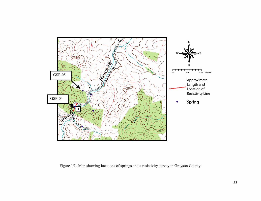
53
Figure 15 - Map showing locations of springs and a resistivity survey in Grayson County.
GSP-04
GSP-05

54
Grayson Co. GSP-042002 Monitoring
Date
5/21/2002 5/25/2002 5/29/2002 6/2/2002 6/6/2002 6/10/2002
Sprin
gflo
w (g
allo
ns p
er m
inut
e)
0.0
0.5
1.0
1.5
2.0
2.5
3.0
Rai
nfal
l (in
ches
)
0.0
0.1
0.2
0.3
0.4
GSP-04 Flow RateRain Gauge Data
Figure 16 - Spring discharge at Spring #04 at the Grayson County site.
55
Figure 17 shows a hydrograph and precipitation for GSP-05 at the Grayson
County site. The second spring shows a much ‘flashier’ response to rain events, and
resembles the hydrographs from the Floyd County site. An isolated rain event was not
captured by the discharge monitoring equipment, and subsequent knowledge of lag times
is unavailable. Lag times (if the system is consistent with the Floyd County site) of
several days are likely. Rainfall events and correlated discharge increases are circled on
Figure 17. α values cannot be calculated for this spring since little qualitative data are
known about the groundwater system at the springhead. In this case the hydrograph
yields only qualitative evidence of a substantial connection to the shallow aquifer through
its apparent rapid response after rain events.

56
Grayson Co. GSP-052002 Monitoring
Date9/2/2002 9/16/2002 9/30/2002 10/14/2002 10/28/2002 11/11/2002
Sprin
gflo
w (g
allo
ns p
er m
inut
e)
0.0
0.2
0.4
0.6
0.8
1.0
1.2
1.4
1.6
Rai
nfal
l (in
ches
)
0.0
0.2
0.4
0.6
0.8
1.0
1.2
GSP-05 Flow RateRain Gauge Data
Figure 17 - Springflow and rainfall at GSP-05 in Grayson County
Figure 18 Detail

57
Grayson Co. GSP-052002 Monitoring
Date10/29/2002 11/2/2002 11/6/2002 11/10/2002 11/14/2002
Sprin
gflo
w (g
allo
ns p
er m
inut
e)
0.0
0.2
0.4
0.6
0.8
1.0
1.2
1.4
1.6
Rai
nfal
l (in
ches
)
0.0
0.2
0.4
0.6
0.8
1.0
GSP-05 FlowrateRaingauge Data
Figure 18 – Figure showing several rain events and probable correlated discharge peaks at GSP-05
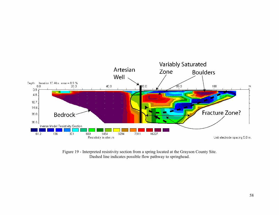
58
Figure 19 - Interpreted resistivity section from a spring located at the Grayson County Site. Dashed line indicates possible flow pathway to springhead.
59
Figure 15 shows the location of a resistivity survey performed in Grayson County,
near GSP-04. Only one survey was conducted at the Grayson Site because of very thick
briers located around other springs. The resistivity line is oriented perpendicular to the
topographic expression of a large fracture/lineament and oriented along the strike of the
rocks in the area. Figure 19 shows the interpreted survey with a distinct bedrock high on
the left (southwest) end of the section. The northeast side of the section is considerably
more complex, showing features such as boulders and a possible fracture zone. The
spring is located in the middle of the resistivity section, and was drilled and cased to a
depth below the maximum depth of investigation for this resistivity survey. The casing
should predetermine the flow path for the spring discharge. If the casing is intact and the
recharge to the deep aquifer system is slow, the hydrograph will be predictably flat (as it
appears in Figure 16). However, if there is rapid recharge to the aquifer supplying the
water to the flowing artesian well, the hydrograph will rainfall related peaks. The
northeast side of the section shows a variably saturated zone that extends from the spring
location to the northeast end of the survey. This zone may have been a previous
contributing flow path for the spring. The casing prevents any fluids from this shallow
aquifer from contributing to the spring discharge. The zone below the spring appears to
be a vertical fracture zone, a possible connection to a deep aquifer system. Spring
discharge data confirm the resistivity observation of no direct connection to a shallow
aquifer system.
The hydrograph analysis method has helped determine possible flow paths for
springs GSP-04 and GSP-05 in Grayson County. In the case of GSP-04, the flow path
was known to be through the deep system, with little to no input from the shallow
60
aquifer. The hydrograph confirmed this, showing a near constant discharge. GSP-05 was
believed to be mostly shallow or a mixed shallow and deep system because of its
intermittent flow. The hydrograph has provided evidence of a shallow flow path, through
the rapid response after a rain event, and a deeper or intermediate flow path by the
sustained discharge after rainfall events.
Summary and Conclusions
Perennial springs have been described and used as drinking water supplies for
many decades in the Blue Ridge Physiographic Province. CFC data have been used to
show that at least two different ages of water exist, modern (less than 30 years old) and
old (greater than 30 years old). These two types of groundwater are contained within a
shallow and deep aquifer, respectively. Anion and cation concentrations in water
samples taken at the Floyd County site confirm this relationship, with higher
concentrations of mean equivalent ions in water with longer residence times in the deeper
aquifer system. Observations of springs using hydrophysical and hydrochemical tools
suggested that some springs may be partly sourced in the shallow aquifer and are
susceptible to drought, while others may be sourced in the deep aquifer and are less
susceptible to drought. Monitoring of spring discharge at both the Floyd and Grayson
sites has shown that some springs display fast (2-4 days) responses to rain events,
indicating that water has flowed very quickly to the spring outlet after a rain event, or that
the recharge area is in close proximity. Other springs have shown very little change in
discharge after rain events, suggesting that their source water flows very slowly to the
spring outlet or the recharge zone is far away. Still other springs show a mixed flow
system with both shallow and deep sources shown as peaks after rain events, and
61
sustained near constant baseflow discharge, even during drought. Electrical resistivity
characterization of geology and hydrology has supported these interpretations. An
aquifer test performed at the Floyd County site also confirmed the connection between
the deep aquifer system and a spring outlet.
This investigation has shown the springflow hydrograph analysis method is useful
for describing different flow paths that may be supplying water to a spring outlet in the
Blue Ridge Physiographic. The hydrograph recession analysis method has shown that
springs in the Blue Ridge Province, in some instances, behave similar to previously
evaluated springs in fractured chalk aquifers in the Middle East, having nearly identical
recession coefficients indicating similar recession time periods possibly through
hydraulically similar aquifer materials. However, the method is not suited to providing
quantitative aquifer parameters in the studied area because of the necessary body of
apriori knowledge that is necessary to quantitatively analyze hydrographs. However, the
hydrograph analysis method can provide substantial qualitative evidence about water
sources for spring outlets. The method can be used to show whether a spring source
originates from deep aquifers that are less susceptible to surface contamination, or from
shallow aquifers and are more susceptible to surface contamination, or from mixed
systems. Hydrograph data combined with geophysical data from surface resistivity and
borehole logs, chemical data, and physical aquifer test data can be used to describe details
of the flow paths, including subsurface geometry.
62
References
Amit, H., V. Lyakhovsky, A. Katz, A. Starinsky, and A. Burg, 2002, Interpretation of Spring Recession Curves: Ground Water, v. 40, 543-551.
Baedke, S. J., and N. C. Krothe, 2001, Derivation of Effective Hydraulic Parameters of a Karst Aquifer from Discharge Hydrograph Analysis: Water Resources Research, v. 37, 13-19.
Clark, G. M., E. J. Ciolkosz, J. S. Kite, and D. A. Lietzke, 1989, Central and Southern Appalachian Geomorphology- Tennessee, Virginia, and West Virginia.
Crockett, C. W., 1971, Climate of Virginia, Silver Spring, National Oceanic and Atmospheric Administration, 17.
Dietrich, R. V., 1959, Geology and Mineral Resources of Floyd County of the Blue Ridge Upland, Southwestern Virginia: Bulletin of the Virginia Polytechnic Institute Engineering Experiment Station Series No. 134: Blacksburg, 160.
Johnson, P., 1999, A Double-Porosity Model of Ground-Water Flow in the Madera Formation Based on Spring Hydrographs and Aquifer Test Analyses from Placitas, New Mexico: New Mexico Geological Society fiftieth annual field conference, Albuquerque, NM, United States, Sept. 22-25, 1999, 393-399.
Karasaki, K., B. Friefeld, A. Cohen, K. Grossenbacher, P. Cook, and D. Vasco, 2000, A Multidisciplinary Fractured Rock Characterization Study at Raymond Field Site, Raymond, CA: Journal of Hydrology, v. 236, 17-34.
Kozar, M. D., C. J. Sheets, and C. A. Hughes, 2000, Ground-Water Quality and Geohydrology of the Blue Ridge Physiographic Province, New River Basin, Virginia and North Carolina, Reston, USGS, 36.
LeGrand, H. E., 1967, Ground Water of The Piedmont and Blue Ridge Provinces in the Southeastern States, Washington, D.C., U. S. Geological Survey, 11.
Loke, M. H., 2002, RES2DINV, Geotomo Software. Loke, M. H., and R. D. Barker, 1995, Least-squares deconvolution of apparent resistivity
pseudosections: Geophysics, v. 60, 1682-1690. Moody, D. W., E. B. Chase, and D. A. Aronson, 1986, National Water Summary 1985 -
Hydrologic Events and Surface-Water Resources, Washington, D.C., U. S. Geological Survey, United States (USA), 506.
Popek, J. P., 1974, An Analysis of the Precambrian Mount Rogers Formation, Grayson Highlands State Park, Grayson County, Virginia: Masters thesis, University of South Florida, Tampa, 98.
Rankin, D. W., 1970, Stratigraphy and Structure of Precambrian Rocks in Northwestern North Carolina, in G. W. Fisher, F. J. Pettijohn, J. C. Reed, Jr., and K. N. Weaver, eds., Studies of Appalachian Geology: Central and Southern: New York, Intersceince Publishers, 227-245.
Seaton, W. J., 2001, Communication Regarding Structural Setting and Hydrogeology of Floyd County, Virginia, Blacksburg.
Seaton, W. J., 2002, Aquifer Characterization in the Blue Ridge Physigraphic Province: PhD Dissertation thesis, Virginia Tech, Blacksburg, 69.
Seaton, W. J., and T. J. Burbey, 2000, Aquifer Characterization in the Blue Ridge Physiographic Province Using Resistivity Profiling and Borehole Geophysics:
63
Geologic Analysis: Journal of Environmental and Engineering Geophysics, v. 5, 45-58.
Seaton, W. J., and T. J. Burbey, 2002, Evaluation of two-dimensional resistivity methods in a fractured crystalline-rock terrane: Journal of Applied Geophysics, v. 51, 21-41.
Sharma, P. V., 1997, Environmental and Engineering Geophysics: Cambridge, Cambridge University Press, 475.
SPSS, I., 2001, SigmaPlot 2001, SPSS, Inc. Thornbury, W. D., 1965, Regional Geomorphology of the United States: New York, John
Wiley & Sons, Inc., 609. United States Census Bureau, 1990, Census of Population and Housing - Summary Tape
File 3 (STF 3), United States Census Bureau. United States Geological Survey, 1963, Check Quadrangle, Virginia: United States
Geological Survey. United States Geological Survey, 2001, Digital Elevation Model of Elk Creek
Quadrangle, Virginia: United States Geological Survey. Virginia Division of Mineral Resources, 1993, Geologic Map of Virginia: Virginia
Division of Mineral Resources.
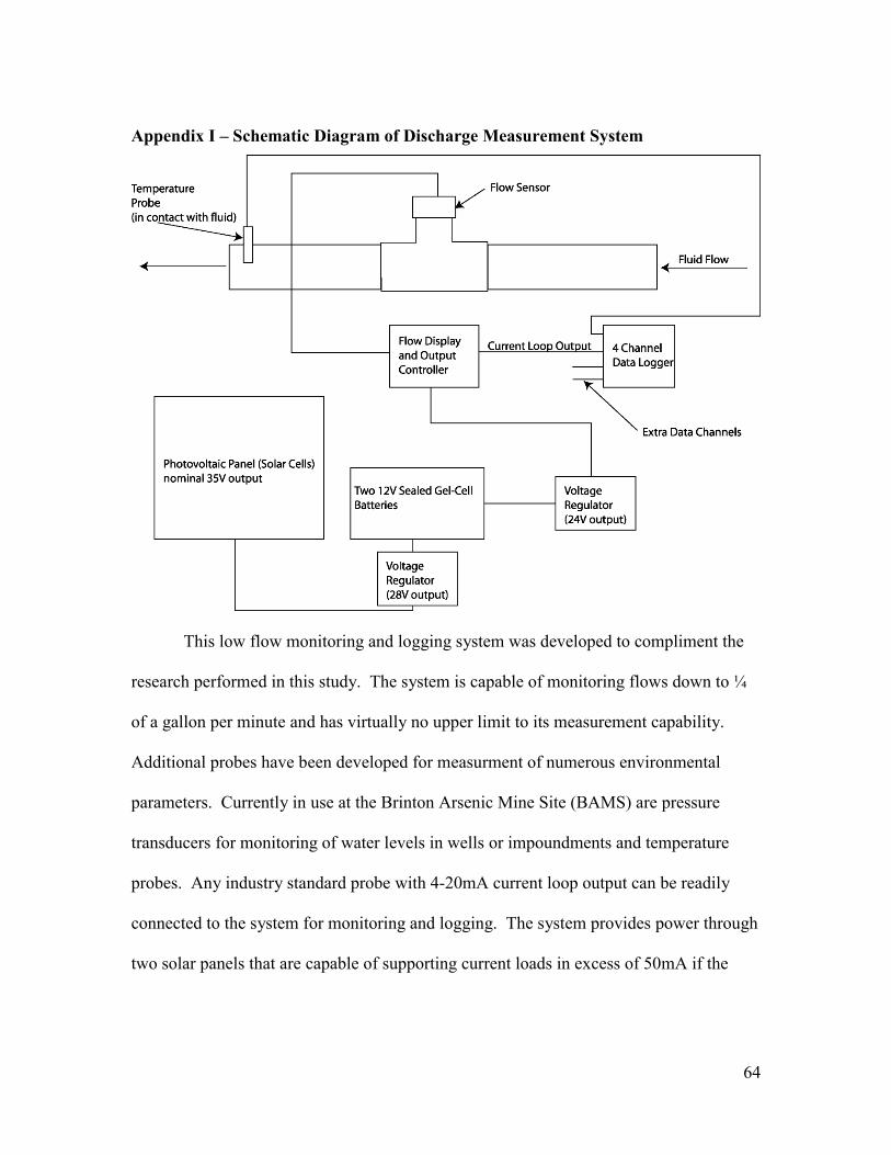
64
Appendix I – Schematic Diagram of Discharge Measurement System
This low flow monitoring and logging system was developed to compliment the
research performed in this study. The system is capable of monitoring flows down to ¼
of a gallon per minute and has virtually no upper limit to its measurement capability.
Additional probes have been developed for measurment of numerous environmental
parameters. Currently in use at the Brinton Arsenic Mine Site (BAMS) are pressure
transducers for monitoring of water levels in wells or impoundments and temperature
probes. Any industry standard probe with 4-20mA current loop output can be readily
connected to the system for monitoring and logging. The system provides power through
two solar panels that are capable of supporting current loads in excess of 50mA if the

65
solar panels receive direct light for a majority of daylight hours. More current capacity is
available by upgrading the solar cells to 10watt or larger capacity panels.

66
Appendix II – Dipole-Dipole Array Details
The Campus Geopulse is an automated resistivity profiling system, capable of
making resistivity measurements that may be converted into resistivity pseudosections.
The system consists of a laptop controlled resistivity meter (labeled Geopulse), which is
connected to a twenty five electrode resistivity cable. Electrodes are planted in the soil at
even spacings (in most cases either 5 or 10m) and a series of measurements are taken.
For this study, the dipole-dipole array was selected. The dipole-dipole array supplies a
current to two electrodes while taking a potential (voltage) reading between another pair
of electrodes. The spacing between the two dipoles (n*a) is widened with each
successive pass down the resistivity cable, resulting in imaging of deeper subsurface
features. The a spacing remains constant throughout the survey. Potential measurements

67
are converted to resistances and ultimately resisitivities by software contained on the
laptop controlling the Geopulse.

68
Appendix III – Resistivity Inversion Parameters
Initial damping factor 0.3000 Minimum damping factor 0.0300 Line search option 2 Convergence limit 1.0000 Minimum change in RMS error 0.4000 Number of iterations 10 Vertical to horizontal flatness filter ratio 1.0000 Model for increase in thickness of layers(0=default 10, 1=default 25, 2=user defined) 1 Number of nodes between adjacent electrodes 4 Flatness filter type 1 Reduce number of topographical datum points? 0 Carry out topography modeling? 1 Type of topography trend removal 1 Type of Jacobian matrix calculation 2 Increase of damping factor with depth 1.0500 Type of topographical modeling 4 Robust data constrain? 1 Cutoff factor for data constrain 0.0500 Robust model constrain? 1 Cutoff factor for model constrain 0.0050 Allow number of model parameters to exceed datum points? 1 Use extended model? 0
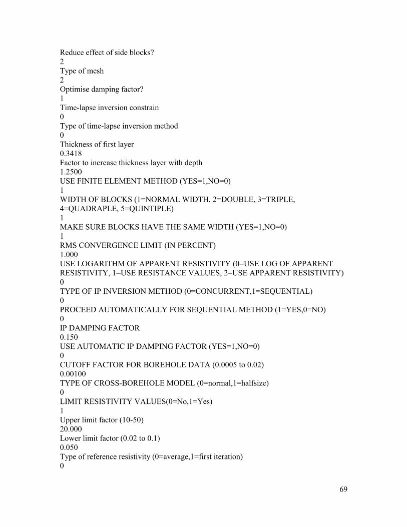
69
Reduce effect of side blocks? 2 Type of mesh 2 Optimise damping factor? 1 Time-lapse inversion constrain 0 Type of time-lapse inversion method 0 Thickness of first layer 0.3418 Factor to increase thickness layer with depth 1.2500 USE FINITE ELEMENT METHOD (YES=1,NO=0) 1 WIDTH OF BLOCKS (1=NORMAL WIDTH, 2=DOUBLE, 3=TRIPLE, 4=QUADRAPLE, 5=QUINTIPLE) 1 MAKE SURE BLOCKS HAVE THE SAME WIDTH (YES=1,NO=0) 1 RMS CONVERGENCE LIMIT (IN PERCENT) 1.000 USE LOGARITHM OF APPARENT RESISTIVITY (0=USE LOG OF APPARENT RESISTIVITY, 1=USE RESISTANCE VALUES, 2=USE APPARENT RESISTIVITY) 0 TYPE OF IP INVERSION METHOD (0=CONCURRENT,1=SEQUENTIAL) 0 PROCEED AUTOMATICALLY FOR SEQUENTIAL METHOD (1=YES,0=NO) 0 IP DAMPING FACTOR 0.150 USE AUTOMATIC IP DAMPING FACTOR (YES=1,NO=0) 0 CUTOFF FACTOR FOR BOREHOLE DATA (0.0005 to 0.02) 0.00100 TYPE OF CROSS-BOREHOLE MODEL (0=normal,1=halfsize) 0 LIMIT RESISTIVITY VALUES(0=No,1=Yes) 1 Upper limit factor (10-50) 20.000 Lower limit factor (0.02 to 0.1) 0.050 Type of reference resistivity (0=average,1=first iteration) 0

70
Vita
W. Miles Gentry
Education B.S., Geological Sciences, 2000, Virginia Tech M.S., Geological Sciences, Virginia Tech Work Summary Mr. Gentry has two years experience in evaluation of aquifer properties using traditional field methods, and using custom manufactured equipment for measuring low discharge spring flow. The investigation involved measurement of spring discharge and resulting hydrographs to evaluate aquifer properties and use of traditional aquifer evaluation techniques including geophysical surface and borehole techniques to confirm the results obtained using the hydrograph method. Mr. Gentry also has experience with numerical modeling of groundwater transport and flow, geophysical inversion modeling, and laboratory analysis of water samples using Dionex DX-120 Ion Chromatograph. Professional Experience January 2001 to Present, Graduate Research/Teaching Assistant, Virginia Tech. As a Master’s student at Virginia Tech, Mr. Gentry designed field equipment to measure and record low spring discharge. Equipment was used in the production of a master’s thesis and is currently used at the Brinton Arsenic Mine Site for environmental monitoring. Other research included analysis of water samples using a Dionex DX-120 Ion Chromatograph to analyze concentration of basic anions. Mr. Gentry also conducted surface geophysical resistivity surveys at four sites and processed the resulting datasets into resistivity pseudosections. These datasets were used to evaluated the springflow hydrograph method as a useful tool for characterization of groundwater resources in the Blue Ridge Province of Virginia. Computer Proficiency Mr. Gentry has experience with document production using Word, Adobe Photoshop, Adobe Illustrator, ArcView 3.2 and ArcMap 8.1. Mr. Gentry also has extensive modeling experience including use of RES2dINV for inversion modeling of resistivity data, ArgusOne/MODFLOW 2000 and GMS for modeling of groundwater flow and transport. Publications Gentry, W. M., and T. J. Burbey, 2002, Analysis of Spring Discharge for Characterization of Groundwater Flow in the Blue Ridge Province, Virginia: Geological Society of America Annual Meeting. Gentry, W.M. and T. J. Burbey, 2001, Blue Ridge Province Spring Characterization: Recent Evidence of Deeper Flow Pathways: Virginia Water Research Symposium.