evaluation of synchronization algorithms with usrp€¦ · evaluation of synchronization algorithms...

Evaluation ofSynchronization Algorithms

with USRP

Martin Lulf

A Thesis submitted for the Degree of

Bachelor of Science

Institute for Communications and Navigation

Prof. Dr. Christoph Gunther

Supervised by Dipl.-Ing. Ronald Bohnke

Munchen, May 2012

Institute for Communications and Navigation Technische Universitat MunchenTheresienstrasse 90

80333 Munich

Abstract

An interface between the Universal Software Defined Radio Peripheral (USRP)and MATLAB has to be developed, as well as a scheme for frequency, delay andphase synchronization to detect received M-PSK symbols after transmission overthe USRPs.

Different methods for the interface implementation are considered and thefinal implementation is done as a shared Mex C++ library that can be accessedfrom within MATLAB like usual functions. The synchronization is done by afeedforward estimator using a BPSK pilot sequence proposed by [1] followed bya delay tracking loop using Gardner’s timing error detector [2, 3] and a phasetracking loop using the Viterbi&Viterbi algorithm [4, 3] for M-PSK signals.Frame synchronization and resolution of the phase ambiguity is done by a Barkercode as start of frame sequence.

It is shown that the feedforward estimator achieves the Cramer-Rao boundsand the following tracking is able to keep the received samples synchronized.Using the MATLAB interface, a set of random data is transmitted over theUSRPs, synchronized and detected at the receiver and compared to the originaldata sequence to validate the single components of this work.

3

Contents

1 Introduction 5

2 Universal Software Defined Radio Peripheral 7

2.1 Overview . . . . . . . . . . . . . . . . . . . . . . . . . . . . . . . 7

2.1.1 USRP1 . . . . . . . . . . . . . . . . . . . . . . . . . . . . 7

2.1.2 Next Generation USRPs . . . . . . . . . . . . . . . . . . . 8

2.1.3 Motherboards . . . . . . . . . . . . . . . . . . . . . . . . . 10

2.1.4 Daughterboards . . . . . . . . . . . . . . . . . . . . . . . . 10

2.2 Interfaces . . . . . . . . . . . . . . . . . . . . . . . . . . . . . . . 11

2.2.1 USRP1 . . . . . . . . . . . . . . . . . . . . . . . . . . . . 11

2.2.2 Next Generation USRPs . . . . . . . . . . . . . . . . . . . 11

2.2.3 Conclusion . . . . . . . . . . . . . . . . . . . . . . . . . . 12

3 MATLAB Interface Implementation 13

3.1 General Considerations . . . . . . . . . . . . . . . . . . . . . . . . 13

3.1.1 Single Thread . . . . . . . . . . . . . . . . . . . . . . . . . 13

3.1.2 Approaches . . . . . . . . . . . . . . . . . . . . . . . . . . 13

3.2 Interface Structure . . . . . . . . . . . . . . . . . . . . . . . . . . 16

3.3 Usage . . . . . . . . . . . . . . . . . . . . . . . . . . . . . . . . . 18

3.3.1 Send and Receive Samples . . . . . . . . . . . . . . . . . . 18

3.3.2 Spectrum Analyzer . . . . . . . . . . . . . . . . . . . . . . 19

4 Synchronization 21

4.1 System Model . . . . . . . . . . . . . . . . . . . . . . . . . . . . . 21

4.2 Feedforward Estimator . . . . . . . . . . . . . . . . . . . . . . . . 23

4.2.1 Joint Maximum Likelihood Estimation . . . . . . . . . . . 24

4.2.2 Frequency Search . . . . . . . . . . . . . . . . . . . . . . . 27

4.2.3 Simulation Results . . . . . . . . . . . . . . . . . . . . . . 28

4.2.4 Synchronization Sequence Detection . . . . . . . . . . . . 30

4.2.5 Measured Results . . . . . . . . . . . . . . . . . . . . . . . 31

4.3 Tracking . . . . . . . . . . . . . . . . . . . . . . . . . . . . . . . . 32

4.3.1 Delay Tracking . . . . . . . . . . . . . . . . . . . . . . . . 34

4.3.2 Phase Tracking . . . . . . . . . . . . . . . . . . . . . . . . 35

4.3.3 Simulation Results . . . . . . . . . . . . . . . . . . . . . . 37

4.3.4 Measured Results . . . . . . . . . . . . . . . . . . . . . . . 37

4.4 Start of Frame Detection . . . . . . . . . . . . . . . . . . . . . . 40

4.5 Data Transmission over the USRPs . . . . . . . . . . . . . . . . . 40

5 Summary 43

A Appendix 45A.1 Send and Receive Multiple Data Streams from a Single Thread . 45A.2 Send and Receive Samples to a File . . . . . . . . . . . . . . . . . 47

A.2.1 Sending Samples . . . . . . . . . . . . . . . . . . . . . . . 47A.2.2 Receiving Samples . . . . . . . . . . . . . . . . . . . . . . 51

A.3 Send and Receive Samples from MATLAB . . . . . . . . . . . . . 54A.4 Spectrum Analyzer . . . . . . . . . . . . . . . . . . . . . . . . . . 55A.5 Available Interface Commands . . . . . . . . . . . . . . . . . . . 57A.6 Derivation of the Maximum Likelihood Estimator . . . . . . . . . 60A.7 Derivation of the Likelihood of Hypothesis Two . . . . . . . . . . 62

5

Chapter 1

Introduction

When investigating new signal processing schemes the simulation of all relevantparameters is a useful tool to get a better understanding of the investigatedsystem. Programmable numerical math software like MATLAB or Octave arewell suited for these simulations as they already have functions for most ofthe mathematical problems as well as for graphical visualization of data, sothe implementation of the simulation can focus on the signals and processingalgorithms themselves.

After successful simulations it is often desirable to test the algorithms in areal world scenario in order to ensure that there have been no wrong assump-tions in the simulations and the algorithms work in a complete communicationsystem. Software defined radios (SDRs) allow the transmission of a wide vari-ety of signals and can thus be easily adopted to such tests. In Chapter 2 theUniversal Software Defined Radio Peripherals (USRP), a software defined radioproduct family by Ettus Research and National Instruments, are described touse them for testing.

If the SDRs can be accessed from the same software that was used for thesimulations, another advantage over specialized RF hardware is that signal pro-cessing code from the simulations can be reused. In Chapter 3, an interface fromMATLAB to the USRPs is developed so MATLAB code can directly access theUSRP devices for testing.

While simulations can simulate special aspects of the communication system,when using SDRs, all aspects of a communication system have to be considered.The often made assumption of coherent detection is not directly possible forreal measurement data. The received samples have to be synchronized first tocontinue with a coherent detection. In Chapter 4, a synchronization scheme isdiscussed which removes carrier frequency and phase offsets as well as timingerrors after transmission over USRPs based on a maximum likelihood feedfor-ward estimation for an acquisition, followed by a feedback tracking loop usinga Gardner timing error detector and the Viterbi&Viterbi phase error detectorto follow further changes of the timing and phase for arbitrary M-PSK modu-lated data. These synchronization schemes allow the test of the work from theprevious chapters both in simulation and with real measured data from USRPs.Additionally they can be used for future works to transmit data symbols overthe USRP and focus on the received coherent samples without worrying aboutsynchronization.

7

Chapter 2

Universal Software DefinedRadio Peripheral

The Universal Software Defined Radio Peripheral (USRP) family are softwaredefined radios that allow transmission and reception of arbitrary baseband sig-nals. Due to the modularization into a mother- and daughterboard they can beadopted to a wide range of operating frequencies. The USRP daughterboardsare responsible for modulation and antialiasing filtering and the motherboardsare dealing with amplification, up- and down converting, decimating and in-terpolating operations that require high processing power but little knowledgeabout the signal itself in a Field Programmable Gate Array (FPGA). All wave-form dependent operations and signal processing focused part are done on a PCwhich enables a high variety of transmission systems with the same hardware.

The USRPs can either sample a signal mixed to an intermediate frequencywith one sinusoidal signal which results in a one dimensional real valued discretesignal or use the orthonormal property of a sine and a cosine wave to samplethe Inphase and Quadrature component individually on two channels to get acomplex1 two dimensional discrete signal.

2.1 Overview

Initially Ettus started with one SDR, the USRP1 device. After its success newerUSRP devices with more features were developed. The next two subsections willgive an overview about the different devices in the USRP family.

2.1.1 USRP1

The first generation, the USRP1 has four input and four output channels andis connected via USB2. The USRP1 can contain two daughterboards and allstreams together can share a data rate of 8 complex mega samples per second[5]. With a few hardware modifications an external 10MHz oscillator can be

1Where the real part corresponds to the Inphase component and the imaginary part to thequadrature component

2Universal Serial Bus 2.0 with a maximum data rate of 32 MByte per second [5]

8CHAPTER 2. UNIVERSAL SOFTWAREDEFINED RADIO PERIPHERAL

Figure 2.1: USRP1 device equipped with one daughterboard connected to twoRF antennas and no external clock connected.

connected to the USRP to provide a more stable oscillator. Figure 2.1 shows aUSRP1 device with no external clock and one daughterboard.

2.1.2 Next Generation USRPs

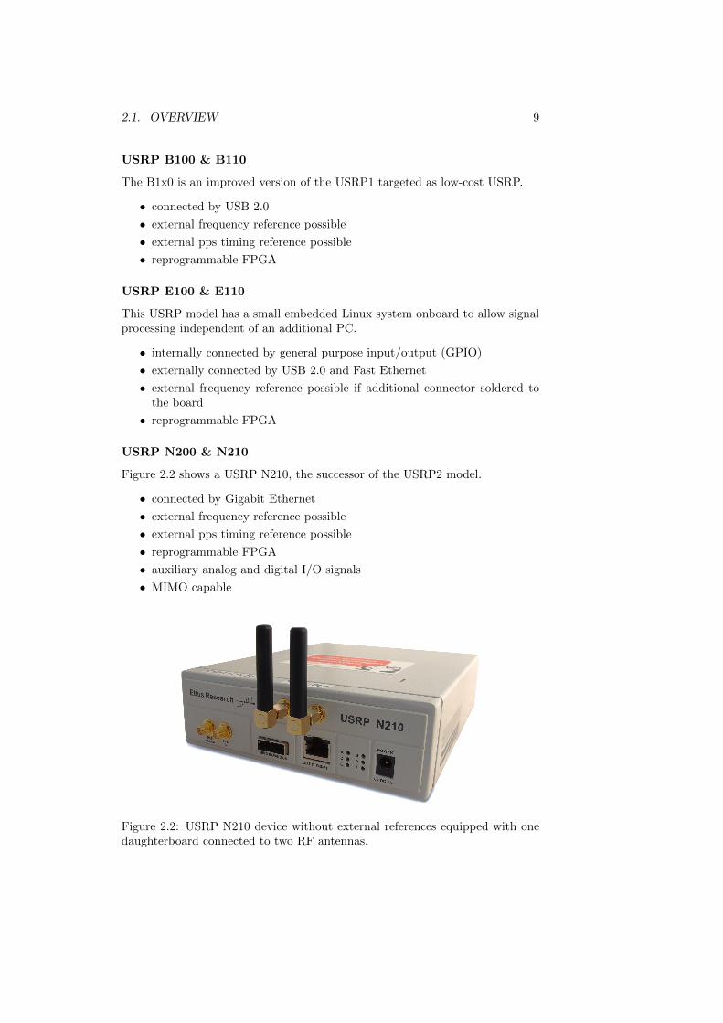
The second generation of USRPs consists of a few different devices with similarproperties. These new USRP devices can hold only one daughterboard and havetwo input and two output channels. Their FPGAs can be reprogrammed formore control of the data processing before decimation and transmission to thePC. Beside the USRP2, each model comes with two versions (e.g. USRP N200& N210) where a tailing 10 in the model number indicates a larger FPGA thanin the tailing 00 models which gives more space for custom preprocessing code.

The next generation USRP devices can be connected with an external os-cillator for a more stable frequency and an external pulse generator for a moreprecise timing reference. These USRP devices can switch between the differ-ent oscillation references and the different timing references (internal, external,MIMO3) via software. The new USRP devices can tag incoming and outgoingsamples to know when exactly they have been received or have to be send. Thisleads to much higher accuracy in runtime measurements or Time Division Mul-tiple Access (TDMA) systems as the delay introduced by USB or Ethernet doesno longer affect the delay of transmission or measurement of reception time.

USRP2

This model was an improvement of the original USRP1. This USRP model isMIMO capable which means multiple USRPs can be connected and operate asa single USRP with more channels. It is no longer sold in favour of the newerN2x0 devices.

• connected by Gigabit Ethernet

• external frequency reference possible

• external one pulse per second (pps) timing reference possible

• reprogrammable FPGA

• MIMO capable

3Multiple Input Multiple Output using a special MIMO cable to synchronize the USRPs

2.1. OVERVIEW 9

USRP B100 & B110

The B1x0 is an improved version of the USRP1 targeted as low-cost USRP.

• connected by USB 2.0


• external pps timing reference possible


USRP E100 & E110

This USRP model has a small embedded Linux system onboard to allow signalprocessing independent of an additional PC.

• internally connected by general purpose input/output (GPIO)

• externally connected by USB 2.0 and Fast Ethernet

• external frequency reference possible if additional connector soldered tothe board


USRP N200 & N210

Figure 2.2 shows a USRP N210, the successor of the USRP2 model.

• connected by Gigabit Ethernet


• external pps timing reference possible


• auxiliary analog and digital I/O signals

• MIMO capable

Figure 2.2: USRP N210 device without external references equipped with onedaughterboard connected to two RF antennas.


2.1.3 Motherboards

The heart of a USRP is it’s motherboard which handles the communication withthe PC and the signal processing at an intermediate frequency (IF). Daughter-boards described in Section 2.1.4 handle the modulation from the intermediateto the operating frequency.

The input signal that was filtered and modulated to the IF by the daughter-board is first sampled and multiplied with a time discrete cosine wave or a sineand cosine wave for complex samples as shown in Figure 2.3. Afterwards thesignal is again filtered and decimated to cancel out the double frequency partsand reduce the number of samples. The resulting baseband samples are storedin a buffer and transmitted to the PC over the USB or Ethernet interface.

Receive Part

NCO

Decimation

Decimation

I1

I2IF signal2

IF signal1

(a) real samples

NCO

Decimation

Decimation−90◦

Q1

I1

IF signal1

(b) complex samples

Figure 2.3: Reception path in the motherboard for real and complex samples

Transmit Part

At the transmission side the data is received over Ethernet or USB and storedin a buffer. Out of this buffer the samples are upsampled, interpolated andmodulated to the intermediate frequency by a cosine for real samples or a sineand a cosine for complex samples. Then the samples are converted into analogsignals and are send to the daughterboard.

2.1.4 Daughterboards

The operating frequency band of the USRP can be controlled by exchanging thedaughter board. Each daughterboard has access to two RX and two TX channels

2.2. INTERFACES 11

for either one complex or two real valued streams in RX and TX direction withfull duplex capabilities. An oscillator with a fixed frequency of 10MHz on themotherboard is used to generate an oscillator on the daughterboard’s targetfrequency. This oscillator modulates the signal from the operating RX frequencyto the IF and the TX streams from the IF into the operating TX frequency. Forreal valued streams the two streams can be connected to different antennas onthe same operating frequency. Most daughterboards are also capable of filteringthe received signal to suppress aliasing effects.

2.2 Interfaces

Depending on the USRP device there are different ways to access it from severalsoftware distributions.

2.2.1 USRP1

The USRP1 device can be interfaced with a driver provided by Ettus [6]. It is aC++ Interface which can be used to switch between real and complex samples,set the operating frequencies, amplification and send or receive the samples fromthe device’s buffer. There are several software that utilize this interface to allowthe use of USRPs:

GnuRadioA block based open source radio software. A USRP can be used like anyother signal source/sink from within this software. All necessary configu-rations of the USRP are accessible from the USRP block.

GnuRadio companionA graphical user interface to GnuRadio that utilizes the GnuRadio inter-face to the USRP.

MATLABA programmable numerical math software by MathWorks. An inter-face between MATLAB and the USRP1 was developed by Institute forCommunications Engineering (LNT) at Technische Universitat Munchen(TUM). It can set the basic configuration options of the USRP and sendand receive samples to and from a vector.

SimuLinkA MATLAB powered block based signal processing environment. An in-terface to access the USRP as Simulink block is available by the Com-munications Engineering Lab (CEL) at Karlsruhe Institute of Technology(KIT) [7].

2.2.2 Next Generation USRPs

To support the various improvements of the new USRP generation Ettus pro-vided a new driver, the USRP Hardware Driver (UHD) [6]. The UHD is a C++interface and offers the same functionality as the old USRP1 driver with theadditional functionality to


• Switch between oscillation and timing reference sources

• Configure time tagged transmission

• Read out time tags from received samples

• Configure channel and antenna assignment in MIMO configuration

• Transmit and receive a specific number of samples by start and end ofburst flags

• Detection and notification on stream interruptions4

The UHD can also access USRP1 devices where the features from above areemulated in the UHD driver on the PC, except for the start and end of burstcapability which is ignored by the driver if a USRP1 device is accessed. Thisway all USRP devices can be accessed by the UHD with the maximum possiblefunctionality for each device.

Similar to the USRP1 driver there are software distributions that use theUHD to access the USRP devices.

GnuRadioVery similar to the implementation of the old USRP1 driver. Most of thenew functionality has been adopted

GnuRadio companionUses the same interface as GnuRadio. There is no time tagging availablein GnuRadio companion.

MATLAB /SimuLinkMathWorks provides the Support Package for USRP c© Hardware to accessthe USRP from within MATLAB/SimuLink [8]. Although this packageuses the UHD it can only be used for the two network based USRP2 andUSRP N2x0 devices with limited functionality

2.2.3 Conclusion

Although there are two existing Interfaces to access the USRP devices fromwithin MATLAB both of them lack some key features. The USRP1 interfacefrom the LNT can only access USRP1 devices and cannot benefit from the newfunctionality of the UHD, while the MathWorks driver is artificially limitedto network based devices and is also lacking time tagging of samples. Dueto the closed source nature of the support package it is impossible to changethis. At the Institute we have both USRP1 and USRP N210 devices and itis very desirable to use both types of devices with the same codebase. Alsothe possibility of doing accurate range measurements by time tagging is veryappealing. These considerations led to the development of a new MATLABinterface which is described in the following Chapter.

4Such as under- or overflow of buffers and impossible time tags at reception or transmission

13

Chapter 3

MATLAB InterfaceImplementation

As motivated in the previous Chapters, this work will implement an interfacebetween MATLAB and the UHD, which should be able to

• access all types of USRP devices with the same MATLAB code

• receive and transmit simultaneously from the same MATLAB code

• tag the time of incoming and outgoing samples

in a way that the full potential of the UHD can be used.

3.1 General Considerations

3.1.1 Single Thread

MATLAB programs run in a single thread, which means that all operations aredone in sequence and no parallel operations are possible. Therefore it is notpossible to directly interact with the channel as this would lead to interruptionsin the data stream as shown in Figure 3.1a on the next page. Instead theinteraction with the channel needs to be buffered in a memory that is fasterthan the channel data rate. For two data streams the memory needs to be atleast twice as fast as the channel. If the memory is even faster there is someadditional time in the thread to do calculations with the received data andgenerate the transmission samples as shown in Figure 3.1b.

The UHD has an internal buffer for USB/Ethernet operations that is suf-ficient for operating two data streams into a single thread. The C++ code inAppendix A.1 on page 45 demonstrates the parallel reception and transmissionfrom a single thread.

3.1.2 Approaches

It is not possible to access the UHD library directly in MATLAB as there is noway of using C++ libraries and data structures from within MATLAB. Howeverthere are a few different approaches that have been taken and are discussed inthe following.

14 CHAPTER 3. MATLAB INTERFACE IMPLEMENTATION

transmission channel

reception channel

Matlab thread

5/0 samples 5/5 samples 10/5 samplesreceived from channelsamples send /

(a) single thread without buffer

transmission channel

reception channel

transmission buffer

reception buffer

Matlab thread

5/3 samples 10/8 samples 15/13 samplesreceived from channelsamples send /

(b) single thread with buffer

Figure 3.1: Channel access with and without buffering in between. Withoutbuffering each channel is empty for half of the time for a single thread.

C/MEX Wrapper

MATLAB can call plain C libraries which can handle C++ code and it is pos-sible to write special C++ code that can be executed from MATLAB1. Boththe C library as well as the MEX code would then work with the C++ libraryinternally and wrap the data into C/MATLAB data structures for further pro-cessing.

This approach is the most direct one compared to the two following ap-proaches, as it directly interacts with the MATLAB data. In the beginning thisclose interaction led to errors with incompatibilities between the Boost library2

used by the system and the ones used within MATLAB3. If these versions do notmatch, the attempt to call the UHD library from MATLAB either by a MEXfile or by calling a wrapping C library loads the Boost version deployed withMATLAB instead of the system’s one which results in a segmentation violation.

1MATLAB Executables (MEX) code that has to be compiled with special compiler optionsand only returns MATLAB compatible data structures

2A C++ library for standard operations in C++.3MATLAB R2011b is linked to Boost version 1.44.0

3.1. GENERAL CONSIDERATIONS 15

Because of this problem the two approaches explained below have been con-sidered. After MathWorks’s technical support pointed us to the use of an in-compatible boost version inside MATLAB4 we were able to compile the UHDagainst the same Boost version as MATLAB which resolved the segmentationviolations. After these issues are solved this approach is the most promising andthus is used for the implementation described in Section 3.2 on the next page.

Server/Client Separation

To have a clear separation between the MATLAB and the USRP side to workaround segmentation violation problems, all UHD related tasks can be run as astand alone program which exchanges configuration and samples with MATLABover a local network5.

As MATLAB has no own network access the fact that MATLAB can naivelyrun Java code is exploited. Java has Remote Procedure Calls6 (RPC) thatenable the network separation with almost no implementation effort. Anotheradvantage of Java code is that it is object oriented. This way multiple USRPdevices can be easily addressed with multiple objects. Figure 3.2 shows thebasic principle of this approach.

UHD

USRP

usrp.send(vector)

Matlab

Matlab

Server ClientRPCRPC

EthernetUSB /

Java

Standalone Programm

Network

Figure 3.2: Separation of UHD and MATLAB address spaces by a server /clientmodel.

The intended clear separation of MATLAB and UHD in this approach alsohas the drawback, that there is no common memory. All data between thetwo instances has to be copied before it can be used. This lead to very strongperformance issues. Receiving data with a rate of up to one Megasample persecond was possible without any transmission at the same time, but any higherdata-rates or parallel transmission led to buffer overruns, because the data wasnot transferred fast enough over the interface.

4The use of Boost inside MATLAB is not documented at a prominent place5Preferably over the loopback device that is a pure virtual network that has no data-rate

limit through a physical connection6That allow access from one Java program to data and Methods of another Java Program

over the network without having to specify the interface first


Files

When it is not necessary to react to the received samples, e.g. no acknowledge-ments in the communication, the interface can be relaxed to sending from, andreceiving into a file. Beside the much lower complexity this approach is repro-ducible by just reimporting the received samples. The sample C++ code inlisting A.4 in Appendix A.2.2 on page 51 receives samples and writes them intoa file as a sequence of double values while the sample code listing A.2 reads afile of subsequent complex double values and transmits them over the USRP.The MATLAB code in listing A.5 shows how to import this data into MATLABand listing A.3 shows how to export it.

3.2 Interface Structure

The whole interface is implemented in a single mex function. This way allnecessary data is available to all functions and only has to be kept persistentbetween subsequent calls of the same Mex function. To tell the Mex functionwhat it should do during a specific call, a command has to be passed to thefunction. To access multiple USRPs in a non object orientated manner eachUSRP object is assigned with an unique integer index at initialization whichis returned to MATLAB. By passing this index together with a command, theMex function can search the right USRP object corresponding to the index andcall the desired function of that object. Listing 3.1 shows the general structureof this function.

The entry point of the Mex function is at line 22. As MATLAB can clearMex function out of memory at any time to ensure that the data is persistentbetween two calls a Mex function can lock itself. A locked Mex function is notcleared from memory unless it is unlocked again, or MATLAB exits. If the Mexfunction is not locked in line 25 it initializes itself by locking and registering amessage handler, which is called by the UHD library to exchange messages. Asthe UHD uses multiple threads it has to be ensured that the message exchangebetween UHD and the single threaded Mex function is Thread safe. At eachcall to the message handler, in line four, a message is appended to a buffer. Amutex7 ensures that either the Mex function or the UHD is accessing the buffer,but not both at the same time. At each call to the Mex function the messagebuffer is read and the messages are printed to the MATLAB console in line32. Afterwards the input parameters are checked for existence and sanity. Theinterface expects at least one input string with the command to call. If there isat least one USRP object initialized, but no USRP index given the first USRPobject (index 0) is used by default, otherwise the USRP index is expected beforethe command string. After the command string an optional third parametercan be given as parameter to the command, e.g. the frequency when settingthe centre frequency of a USRP. In lines 43 to 67 all possible commands arechecked in sequence and executed if all conditions for a command are fulfilled.After a command is executed the Mex function returns to MATLAB. When theprogram reaches line 69, no command has been executed and an according errormessage is printed out before returning to MATLAB.

7A programming concept which ensures mutual exclusion

3.2. INTERFACE STRUCTURE 17

Listing 3.1: Structure of the Mex file to achieve access to all functions on mul-tiple USRPs from one Mex function.

1 static uhd::usrp:: multi_usrp ::sptr[] usrp;

2 static boost:: mutex messages_mutex;

3

4 void message_handler(uhd::msg:: type_t type , const std::

string &msg){

5 // ensure messages are not read out during this run

6 boost:: mutex:: scoped_lock lock(messages_mutex);

7

8 // ...

9 // store message

10 // ...

11 }

12

13 void process_messages(void) {

14 // ensure messages are not stored during this run

15 boost:: mutex:: scoped_lock lock(messages_mutex);

16

17 // ...

18 // print out stored messages

19 // ...

20 }

21

22 extern "C" void mexFunction(int nlhs , mxArray *plhs[], int

nrhs , const mxArray *prhs []) {

23

24 // make sure we do not get cleared without our permission

25 if(! mexIsLocked ()) {

26 // lock the file

27 mexLock ();

28 // register message handler so errors can be printed out

29 uhd::msg:: register_handler (& message_handler);

30 }

31 // read out messages , that arrived during time in Matlab

32 process_messages ();

33

34 // ...

35 // check inputs

36 // ...

37

38 int uhd = getUInt(prhs [0]);

39 std:: string command = getString(prhs [1]);

40 const mxArray *arg = prhs [2];

41

42 // check individual commands

43 if(command.compare("init") == 0) {

44 std:: string devarg = getString(arg);

45 uhd::usrp:: multi_usrp ::sptr usrp_local = uhd::usrp::

multi_usrp ::make(devarg);

46 // ...

47 // store usrp_local at i-th position in usrp[]

48 // ...

49 plhs [0] = retInt(i);


50 return;

51 }

52 // only possible if the given USRP is initialized

53 if(command.compare("set_rx_frequency") == 0 and usrp[uhd])

{

54 usrp[uhd]->set_rx_freq(getDouble(arg));

55 return;

56 }

57 // ...

58 if(command.compare("exit") == 0) {

59 // unlock Mex function so it can be cleared

60 mexUnlock ();

61 return;

62 }

63 if(command.compare("flush") == 0) {

64 // do nothing , just print out new messages

65 // from the UHD , which has been done above

66 return;

67 }

68

69 // nothing to do yet :(

70 mexErrMsgIdAndTxt( "MATLAB:uhdInterface:noCommand", "

Please specify a command");

71 return;

72 }

3.3 Usage

To use the interface, the compiled mex code needs to be accessible to MATLAB.On a new system it might be necessary to compile the code with the make.mMATLAB script. Afterwards the binary file uhdinterface.mex*** 8 needs tobe added to MATLAB’s path. The interface can then be used by a call touhdinterface from within MATLAB. Section A.5 on page 57 lists every possiblecommand of the interface.

3.3.1 Send and Receive Samples

The sample code in listing A.6 in Appendix A.3 on page 54 shows how to sendand receive samples over the interface and demonstrates the usage of the mostcommon commands of the interface. In lines two and three the two used USRPsare initialized and their index values are stored in the two variables uhdsend anduhdrecv. Instead of sending from one USRP to another one it is also possibleto transmit and receive from the same USRP. In this case only one USRPobject has to be initialized and both the transmission as well as the receptioncommands need the index of the same USRP object as argument. In lines sixto eleven the parameters of the transmission are set. The frequencies are givenin Hertz, the data rates in samples per second and the gains in the range fromzero to 30 dB. Whenever parameters which are not possible with the USRPs are

8The exact file suffix depends on the used operating system and the computer’s architec-ture.

3.3. USAGE 19

given the UHD notifies the user. To show the output of the last command inline eleven the output of the UHD is flushed to the MATLAB console in line 14.Afterwards the number of received and transmitted samples is set and the sendand receive buffers are initialized. In line 27 the reception of samples is startedand in line 28 the transmission of samples is started. Unless otherwise configuredthe transmission from the internal sample buffer starts 100ms after the call ofthis function. As the USRP needs some time during its transient state the firstreceived samples are useless and are thrown away in line 32. If it is important toreceive even the first transmitted bit it is possible to send zero symbols beforethe actual message to give the USRPs some time to tune in. The main receptionloop starts at line 35. In this example a constant symbol is transmitted so itis not necessary to recalculate the send buffer. The previous send buffer isretransmitted in line 36. In line 37 the next set of samples is received andstored into the reception buffer. In line 45 and 46 the two initialized USRPsare closed again and if no other USRP device is initialized the interface unlocksitself. When using the same USRP device for transmission and reception thisdevice has to be closed only once.

3.3.2 Spectrum Analyzer

The USRP interface can also be used to display the spectrum of the receivedsamples. Figure 3.3 on the next page shows the spectrum of an ECSS9 com-patible ranging and telecomand signal generated by [9]. The according code isshown in listing A.7 on page 55 in the Appendix. While permanently receivingsamples, their discrete Fourier transform is computed and averaged over a shorttime period. The resulting spectrum is plotted and updated in a configuredinterval. By using MATLAB for this task it is possible to view the spectrumthrough the same hardware as a sample code would do and it is possible tozoom and pan the spectrum like any other plot in MATLAB while it is stillbeing updated.

9European Cooperation for Space Standardization


(a) Overall spectrum of an ECSS compatible ranging and telecom-mand signal.

(b) Zoomed in detail of a side peak of an ECSS compatible rangingand telecommand signal.

Figure 3.3: Screenshots of a spectrum analyzer implemented in MATLAB usingthe USRP interface

21

Chapter 4

Synchronization

When transmitting a signal it is in general modified by the channel beforereception. This work will assume an additive white Gaussian noise (AWGN)channel. Beside the additive noise whose effect is shown in Figure 4.1a onthe following page, the signal also needs its time to propagate through thischannel which is seen as a delay at the receiver side and can lead to samplingat suboptimal time instances as shown in Figure 4.1b. Because of the Dopplershift due to relative movements between sender and receiver and because ofimperfections in their local oscillators the signal is also rotated in the signalspace by a constant frequency offset as shown in Figure 4.1c as well as by aconstant rotation because of a phase offset in the local oscillators and the signalpropagation as shown in Figure 4.1d.

All these effects lead to a modification of the send signal at the receiver side.Synchronization aims at estimating the frequency offset and channel delay, aswell as the phase offset in a coherent receiver to remove or at least reduce themodifications before the detection of the sent data symbols.

4.1 System Model

Starting with the N data symbols d[i] ∈ D ⊂ C the baseband transmissionsignal s is formed by the root-raised cosine transmit filter gT

s(t) =

N∑i=1

d[i] · gT (t− iT ) . (4.1)

The baseband signal s is then modulated to the carrier frequency fs with anarbitrary phase of the local oscillator φs resulting in the analytic representationof the real valued send passband signal sRF at radio frequency

sRF (t) = s(t) · ej(2πfst+φs). (4.2)

After transmission over the AWGN channel the signal at the receiver ismodelled with a transmission delay t′ and a noise term wRF with one-sidedpower spectral density N0

rRF (t) = sRF (t− t′) + wRF (t)

= s(t− t′) · ej(2πfs(t−t′)+φs) + wRF (t). (4.3)

22 CHAPTER 4. SYNCHRONIZATION

−1 −0.5 0 0.5 1

−1

−0.8

−0.6

−0.4

−0.2

0

0.2

0.4

0.6

0.8

1

Inphase component

Qua

drat

ure

com

pone

nt

Signal constellation with different noise variances

σ2 = 0

σ2 = 0.008

(a) Additive white Gaussian noise offsets the samplesaround the send data symbol

−1 −0.5 0 0.5 1

−1

−0.8

−0.6

−0.4

−0.2

0

0.2

0.4

0.6

0.8

1

Inphase component

Qua

drat

ure

com

pone

nt

Signal constellation with constant delays τ

τ = 0τ = 0.137

(b) Propagation delay leads to sampling at suboptimaltime intervals

−1.5 −1 −0.5 0 0.5 1 1.5

−1

−0.5

0

0.5

1

Inphase component

Qua

drat

ure

com

pone

nt

Signal constellation with constant frequency offset ν = 0.0413

5 10 15 20 25 30 35 40 45 50

(c) Frequency offset continuously rotates the received sam-ples

−1 −0.5 0 0.5 1

−1

−0.8

−0.6

−0.4

−0.2

0

0.2

0.4

0.6

0.8

1

Inphase component

Qua

drat

ure

com

pone

ntSignal constellation with constant phase offsets φ

φ = 0φ = −0.355

(d) Phase offset rotates the samples by a constant angle

Figure 4.1: Influences of the delayed AWGN channel on a BPSK signal

This received signal is then downmodulated with a frequency fr similar tofs. Because of differences in the local oscillators at sender and receiver sideand because of the Doppler shift due to relative movement between sender andreceiver fs and fr are in general not identical. φr is an arbitrary phase of thelocal oscillator at the receiver

r(t) = rRF (t) · e−j(2πfrt+φr). (4.4)

Withw(t) := wRF (t) · e−j(2πfrt+φr) (4.5)

equation (4.4) becomes

r(t) = s(t− t′) · ej2π(fs−fr)t · ej(φs+φr−2πfst′) + w(t). (4.6)

The received signal is filtered with a root raised cosine low pass filter witha one-sided bandwidth of 1

2Tsthat limits the noise, but keeps the signal undis-

4.2. FEEDFORWARD ESTIMATOR 23

torted. Sampling the filtered signal with a frequency of 1Ts

leads to

r[k] = r(kTs) = s(kTs − t′) · ej2π(fs−fr)kTs · ej(φs+φr−2πfst′) + w(kTs) (4.7)

with

w(kTs) ∝ NC

(0, σ2 =

N0

Ts

). (4.8)

To come to a simpler notation and eliminate the units the following normal-ization is applied. The oversampling factor Nos is defined as the ratio betweenthe symbol interval T and the sampling interval Ts

Nos :=T

Ts. (4.9)

The normalized delay D is defined as

D :=t′

T(4.10)

which is divided into the integral delay η and the fractional delay τ . In thiswork, only the fractional delay is considered and the integral delay is assumedto be zero, as the integral delay has no impact on synchronization and onlyintroduces a delay in the received symbols

D = η + τ , τ ∈ [−0.5, 0.5) ∧ η ∈ N. (4.11)

The frequency offset is normalized by the symbol interval and is consideredto be limited

ν = (fs − fr)T , ν ∈ [−0.5, 0.5). (4.12)

The phase offset is collected in a single variable φ0

φ0 = φs + φr − 2πfsDT , φ0 ∈ [−π, π). (4.13)

Applying the normalizations from (4.9) to (4.13), equation (4.7) becomes

r[k] = s(

(k −Nosτ)Ts

)· ej2π

νkNos · ejφ + w(kTs). (4.14)

4.2 Feedforward Estimator

In [1] a feedforward synchronization scheme is presented that will be used inthis work. It is designed for burst mode transmission where the time betweenthe reception of the first sample and the time of correct detection of the dataplays an important role. Therefore a synchronization sequence of known datasymbols is transmitted first, followed by a short, known start of frame (SoF)sequence and the message’s data symbols as shown in Figure 4.2 on the nextpage.

The synchronization sequence consists of alternating ±1 BPSK symbols.This sequence optimizes the Cramer-Rao lower bound for timing estimation,because the corresponding spectrum has only two peaks at the maximum fre-quencies. This sequence also decomposes the estimation of the three parameterstiming τ , carrier frequency offset ν and the carrier phase φ into a one dimensional


Synchronization sequence Frame dataStart of Frame

Figure 4.2: Organization of synchronization sequence, start of frame sequenceand the message’s data symbols.

frequency search as shown in the next Section. While following the derivationsfrom [1] instead of estimating the phase at the beginning of the synchroniza-tion sequence, this work will estimate the phase at the middle of the sequencewhich leads to a lower overall variance of the phase estimation. The algorithmoperates on the received samples with an oversampling factor of two.

4.2.1 Joint Maximum Likelihood Estimation

The probability for a received sample r[k] from equation (4.14) conditionedon fixed synchronization parameters ν, τ and the phase at the middle of thesynchronization sequence φ = φ0 + πνL can be expressed as

p(r[k] | s, ν, τ , φ) =1

πσ2exp

(− 1

πσ2

∣∣∣r[k]− s ((k −Nosτ)Ts) ej(2π νk

Nos+φ)∣∣∣2) .(4.15)

When transmitting the synchronization sequence of alternating ±1 the re-sulting filtered spectrum consists of two peaks at ± 1

2T which corresponds to acosine. Thus, the bandlimited continuous form of the send signal s(t) can alsobe written as

s(t) =√Nos cos

(πt

T

)(4.16)

Because of the independence of the individual samples, the likelihood func-tion for the synchronization sequence of length L given the synchronizationparameters ν, τ and φ can be expressed as the product of all 2L samples

p(r[k] | s, ν, τ , φ) =

2L−1∏k=0

1

πσ2exp

(− 1

πσ2

∣∣∣∣r[k]−√Nos cos

(πk

Nos− πτ

)ej(2π

νkNos

+φ)∣∣∣∣2).

(4.17)

To fulfil the maximum likelihood principle, the parameters ν, τ and φ arechosen such that the likelihood function (4.17) is maximized

(ν, τ , φ) = arg maxν,τ ,φ

{p(r[k] | s, ν, τ , φ)

}. (4.18)

Instead of maximizing p directly the logarithmic likelihood function Λ =ln(p) is maximized

Λ(r[k] | ν, τ , φ) =− 2L ln(πσ2

)− 1

πσ2

2L−1∑k=0

∣∣∣∣r[k]− ej(πν(k−L)+φ)√Nos cos

(πk

Nos− πτ

)∣∣∣∣2 .(4.19)


When leaving out constant parts, equation (4.19) transforms to

ψ(ν, τ , φ) =−2L−1∑k=0

∣∣∣∣r[k]− ej(πν(k−L)+φ) ·√Nos cos

(πk

Nos− πτ

)∣∣∣∣2

=−2L−1∑k=0

(r[k]− ej(πν(k−L)+φ) ·

√Nos cos

(πk

Nos− πτ

))·(r∗[k]− e−j(πν(k−L)+φ) ·

√Nos cos

(πk

Nos− πτ

))=−

2L−1∑k=0

|r[k]|2 +Nos cos2(πk

Nos− πτ

)− 2√Nos<

{r[k] · e−j(πν(k−L)+φ) · cos

(πk

Nos− πτ

)}. (4.20)

Using the two times oversampled signal (Nos = 2), equation (A.6.1) on page60 shows, that the sum over the squared cosine term is independent of ν, τand φ. Therefore, again omitting constant terms, the maximization of (4.20) issimplified as

Ψ(ν, τ , φ) =<

{e−j(φ−πLν)

2L−1∑k=0

r[k] · e−jπkν · cos

(πk

2− πτ

)}.

Regrouping the samples into odd and even ones leads to

Ψ(ν, τ , φ) =<

{e−j(φ−πLν) ·

( L−1∑k=0

r[2k] · e−jπ2kν · cos

(π2k

2− πτ

)

+

L−1∑k=0

r[2k + 1] · e−jπ(2k+1)ν · cos

(π (2k + 1)

2− πτ

))}

=<


( L−1∑k=0

r[2k] · e−jπ2kν · cos (πk − πτ)

+

L−1∑k=0

r[2k + 1] · e−jπ2kν · e−jπν · cos(πk +

π

2− πτ

))}

=<


( L−1∑k=0

r[2k] · e−jπ2kν · (−1)k · cos (πτ)

+

L−1∑k=0

r[2k + 1] · e−jπ2kν · e−jπν · (−1)k · sin (πτ)

)}. (4.21)

Naming the splitted received samples in (4.21) as

Ye(ν) :=

L−1∑k=0

(−1)k · e−j2πkν · r[2k] (4.22)

Yo(ν) :=

L−1∑k=0

(−1)k · e−j2πkν · r[2k + 1] (4.23)


reveals that these quantities can be computed very efficiently using the fastFourier transformation (FFT). Also this leads to a simpler notation of Ψ

Ψ(ν, τ , φ) = <{e−j(φ−πLν)

[Ye(ν) · cos(πτ) + e−jπν · Yo(ν) · sin(πτ)

]}. (4.24)

Defining the inner part as Z(ν, τ)

Z(ν, τ) := Ye(ν) · cos(πτ) + e−jπν · Yo(ν) · sin(πτ) (4.25)

equation (4.24) can be rewritten as

Ψ(ν, τ , φ) = |Z(ν, τ)| · cos(]Z(ν, τ)− φ+ πLν

). (4.26)

From equation (4.26) the optimum φ for a fixed ν and τ can be observedwhen the cosine term becomes one, which leads to

φ = ]Z(ν, τ) + πLν. (4.27)

Inserting the optimal phase estimate from above, equation (4.26) leads to

Ψ(ν, τ , φ) = |Z(ν, τ)| (4.28)

which has the same maximum as

Γ(ν, τ) =2 ·Ψ2(ν, τ , φ)

=2 |Z(ν, τ)|2 .

Equation (A.6.2) on page 61 shows the equality to

Γ(ν, τ) = |Ye(ν)|2 + |Yo(ν)|2 + <{e−j2πτA(ν)

}(4.29)

with

A(ν) := |Ye(ν)|2 − |Yo(ν)|2 + j2<{ejπνYe(ν)Y ∗o (ν)

}. (4.30)

Equation (A.6.3) on page 62 shows the argument phase notation of A as

A(ν) =∣∣Y 2e (ν) + e−j2πνY 2

o (ν)∣∣ e]A(ν). (4.31)

Inserting (4.31) into (4.29) leads to

Γ(ν, τ) = |Ye(ν)|2 + |Yo(ν)|2 + |A(ν)| cos (]A(ν)− 2πτ)

= |Ye(ν)|2 + |Yo(ν)|2 +∣∣Y 2e (ν) + e−j2πνY 2

o (ν)∣∣ cos (]A(ν)− 2πτ)

(4.32)

which is maximized for fixed ν when the cos term equals to one, which leads to

τ =1

2π]A(ν). (4.33)

When inserting (4.33), equation (4.32) becomes

P (ν) =Γ(ν, τ)

= |Ye(ν)|2 + |Yo(ν)|2 +∣∣Y 2e (ν) + e−j2πνY 2

o (ν)∣∣ . (4.34)


Finally the maximum of the likelihood function can be obtained by a onedimensional search over the frequency offset, which is described in the nextSection, with

ν = arg maxν

{P (ν)} . (4.35)

With the result of the frequency offset search the other two synchronizationparameters can be calculated from (4.33) with A(ν) from (4.30)

τ =1

2π]A(ν) (4.36)

and from (4.27) with Z(ν, τ) from (4.25) with

φ = ]Z(ν, τ) + πLν. (4.37)

4.2.2 Frequency Search

As showed in the previous Section the frequency estimation is achieved by amaximum search over P (ν) which is a combination of the two spectra Ye(ν)and Yo(ν), which can be computed using the FFT algorithm. The spectral res-olution of P is given by the spectral resolution of Ye and Yo, which is givenby the length of the FFT input ye and yo. To increase the spectral resolutionthese input sequences can be enlarged by adding additional zeros at the end.This technique is called zero padding, where a pruning factor K is defined as

−0.5 −0.4 −0.3 −0.2 −0.1 0 0.1 0.2 0.3 0.4 0.50

0.5

1

1.5

2

normalized frequency offset

P(ν)

FFT based frequency search for ν = 0.315 at 0dB SNR

FFT binsFFT bins maximum

0.3146 0.3148 0.315 0.3152 0.3154 0.3156 0.3158 0.316 0.3162 0.31640

2

4

6

normalized frequency offset

P(ν)

DFT based refinement for frequency search

DFT binsDFT bins maximumFFT binsFFT bins maximum

Figure 4.3: Frequency Search principle with a coarse search using the FFTalgorithm and a refinement using the DFT in a second step.

the ratio between the length of the zero padded and the original sequence. By


doubleing the amount of input samples the resolution is doubled, however thecomputational complexity is also more than doubled. The drawback of zeropadding in this work is that the frequency resolution over the whole spectrumis increased while only a high spectral resolution around the maximum is ben-eficial for the maximum frequency search. Thus a lot of computational powerto compute large FFTs is needed as well as the memory to store the refinedFFT for the small benefit of having the frequency refinement also around themaximum.

To overcome this drawback the frequency search is done in more than onestep. First the spectrum of P is computed using the FFT without zero padding.From this spectrum a coarse frequency estimation νc is determined. With knowl-edge of the rough position of the maximum and the assumption that the spec-trum is locally concave around the maximum, the spectrum can be refinedaround the maximum using the discrete Fourier transform (DFT). The fre-quency range around the maximum is divided into 1000 equidistant frequencybins and the DFT of ye and yo for these frequency bins is computed using aDFT matrix. The fine frequency estimate νf can be found by recomputing Pwith the new spectra and taking the maximum as shown in Figure 4.3 on thepreceding page. To further increase the spectral resolution the computed νfcan be considered as another coarse estimation and the previous step can berepeated.

For a productive implementation of the frequency search, instead of comput-ing a DFT matrix and performing the matrix multiplication on every repetition,more performant methods like the golden section search with the Goertzel al-gorithm to compute the single spectral points should be used.

4.2.3 Simulation Results

To evaluate the performance of the synchronization scheme from above, themean squared error (MSE) between uniformly distributed random synchroniza-tion parameters and their estimates is computed for different signal to noiseratios (SNRs). These MSEs are compared to the Cramer-Rao bounds (CRBs)for frequency, phase and timing estimation. The CRB is the theoretical lowerbound of the variance of an unbiased estimator and serves as a reference for aperfect synchronization scheme. The CRBs are computed as [1]:

CRBν =1

SNR· 12

π2L[4L2 − 4 + 3 sin2(2πτ)

] (4.38)

CRBτ =1

SNR· 1

π2L(4.39)

CRBφ =1

SNR· 2 (2L− 1) [4L− 1− 3 cos(τ)]

L[4L2 − 4 + 3 sin2(2πτ)

] (4.40)

The simulated results of the joint MLE are plotted in Figure 4.4 on the nextpage. For each SNR value the MSE is computed for 1000 frequency, timing andphase offsets with an observation length of 1024. The frequency search is donein two different ways. In Figure 4.4a a FFT with a zero padding pruning factorof 64 is used for coarse frequency estimation. In Figure 4.4b the DFT refinementdescribed in the previous Section is used with one repetition. In Figure 4.4athe MSEs hit the CRBs for SNRs up to 8dB. For higher SNRs the frequency


−10 −5 0 5 10 15 20 25 3010

−14

10−12

10−10

10−8

10−6

10−4

10−2

100

SNR [dB]

Var

ianc

e/M

SE

Variance/MSE of the estimated parameters, L=1024, n=1000

MSEν

MSEτ

MSEφ

CRBν

CRBτ

CRBφ

(a) zero padded FFT with pruning factor of 64

−10 −5 0 5 10 15 20 25 3010

−14

10−12

10−10

10−8

10−6

10−4

10−2

100

SNR [dB]

Var

ianc

e/M

SE

Variance/MSE of the estimated parameters, L=1024, n=1000

MSEν

MSEτ

MSEφ

CRBν

CRBτ

CRBφ

(b) DFT refinement repeated once

Figure 4.4: Mean squared errors of the joint maximum likelihood estimatorcompared to the CRBs for different frequency search methods


estimation hits an error floor because of the coarse frequency search. As thephase estimation is strongly dependent on the correct frequency estimation italso exhibits an error floor, while even the very inaccurate frequency estimationsfor high SNRs are good enough to compute an accurate timing estimation. Thusthe MSE for the timing estimation hits the corresponding CRB over the wholesimulated SNR range. In Figure 4.4b the frequency estimation is computedwith a higher accuracy. In this case the MSEs of all three parameters hit theCRBs in the complete simulated SNR range, which means that with the sameparameters any other estimator can only be as good as the discussed joint MLEestimator in terms of estimation accuracy.

4.2.4 Synchronization Sequence Detection

Before starting the maximum likelihood estimation described above on mea-sured data, the receiver first has to detect that the synchronization sequenceis received. Therefore the receiver iterates over small blocks of the receivedsamples (e.g. 64 samples) and checks this sequence for the presence of the syn-chronization data. Equation (4.34) seems suitable for the detection as a syn-chronization sequence creates one distinct peak in P (ν) while noise just raisesthe average value of P (ν). A signal to noise ratio can be calculated by comput-ing the quotient of maxν {P (ν)} as a measure of signal and noise energy andE [P (ν)] as a measure for the noise energy. Once the SNR raises over a thresholdvalue the presence of the synchronization sequence is assumed and the joint MLestimation is started on the following samples.

Unfortunately the USRP devices transmit a strong carrier signal even whentransmitting zero symbols. This carrier signal also creates a distinct peak inP (ν) and thus mimics the presence of a synchronization sequence even whenthe transmission of this sequence has not yet been started. Although from asubsequent view of the SNR estimates an increased SNR is observed when thesynchronization sequence is transmitted due to the higher energy of the synchro-nization data over the carrier, there is no absolute value at which the presenceof a synchronization sequence can be assumed, when not knowing the attenu-ation of the channel. To reliably decide between the presence or absence of asynchronization sequence without knowing the channel attenuation, hypothesistesting instead of SNR estimation is used. The following three hypotheses aremade:

H1 A synchronization sequence is present

H2 A carrier signal, but no synchronization sequence is present

H3 The received samples do not contain a signal, but only noise

The probability of each of these hypotheses under the condition of the re-ceived samples is evaluated and compared to the other ones. Instead of directlycalculating the probability p of each hypothesis a monotonic function Ψ is used


instead, with

Ψ(p) =1

2

(ψ(p) + L+

2L−1∑k=0

|r[k]|2)

=πσ2 ln(p) + 2πσ2L ln(2πσ2

)+

1

2

(L+

2L−1∑k=0

|r[k]|2)

(4.41)

This definition of Ψ comes from the derivation of the maximum likelihood esti-mator with Ψ = Ψ− L

2 from equations (4.17) to (4.21) with ψ being the negativesum of the Euclidean distances between the received samples and the expecteddata symbols in the signal space. The likelihood of hypothesis one can be takenfrom (4.28) as

ΨH1(ν, τ) = |Z(ν, τ)| − L

2(4.42)

ΨH2 is computed in (A.7.1) on page 62

ΨH2(ν) =

∣∣∣∣∣2L−1∑k=0

r[k] · e−jπkν∣∣∣∣∣− L

2(4.43)

For hypothesis three no data symbols are expected, so −ψ is just the norm ofthe received samples and thus

ΨH3 =1

2

(−

2L−1∑k=0

|r[k]|2 +

2L−1∑k=0

|r[k]|2)

= 0 (4.44)

To avoid false detection during transitions between two hypotheses the pres-ence of a synchronization sequence is only assumed when the likelihood of hy-pothesis one is larger than the likelihood of the two other hypotheses plus certainthresholds κ− = 0.05 and κ+ = 1.05, which lead to the following decision criteria

ΨH1 > κ− > 0 = ΨH3 ∧ ΨH1 > κ+ ·ΨH2. (4.45)

Figure 4.5 on the following page shows the calculated likelihoods for twomeasured USRP signals which start transmitting the synchronization sequenceat block number 25. It can be observed that the detection criteria of equation(4.45) will always lead to a clear and correct detection in the plotted cases.

4.2.5 Measured Results

To test the performance of the synchronization scheme over a real channel thesynchronization sequence is transmitted from one USRP device to another. Forhigh SNR cases the data is transmitted over a cable, for lower SNR it is trans-mitted over antennas with low transmit power. As the estimation errors of thesynchronization parameters are hard to measure, the received and correctedsignal constellation is inspected instead, to see if a clear detection is possible.Figure 4.6 on page 33 shows the signal constellation for two data sequences,once after reception and once after synchronization and decimation. It can be


0 5 10 15 20 25 30 35 40 45 50−0.4

−0.2

0

0.2

0.4

0.6

0.8

likelihood of H1 and H2 with a search length of 64

block number

H1 with 10dB amplificationH2 with 10dB amplificationH1 with 10dB attenuationH2 with 10dB attenuationH3

Figure 4.5: Hypothesis testing over subsequent blocks of samples, while switch-ing from transmitting only a carrier to the synchronization symbols at blocknumber 25.

observed that the received samples in Figures 4.6a and 4.6b are not suited fordetection of the transmitted BPSK symbols, while the synchronized samples inFigure 4.6a allow a clear separation of the transmitted symbols. In Figure 4.6aand especially in Figure 4.6b it can be observed that there is still an error inthe frequency estimation which leads to slightly rotating symbols in the signalspace. While this rotation can be neglected for the small number of samplesin Figure 4.6a, the large amount of samples in Figure 4.6b leads to an overallrotation that will make it impossible to detect the correct symbols. In the nextSection, tracking of the received samples is discussed which will correct theseremaining rotations and keep track of the timing estimation.

4.3 Tracking

As discussed in the previous Section, even small errors in the initial synchroniza-tion can lead to detection problems when receiving over longer time instances.But also the parameters themselves can vary over time due to movements aswell as clock drifts between sender and receiver. To compensate for this changesthe receiver does not only estimates the synchronization parameters once, butkeeps track of them and continuously corrects them during further reception. Inthis work the delay and the phase is tracked with two closed loops. Both loopswork with the samples after the matched filter y, while the initial estimation ofthe phase and frequency offset is corrected before the matched filter, the timingerror is preserved and initializes the timing error loop.

4.3. TRACKING 33

−1 −0.5 0 0.5 1

−0.8

−0.6

−0.4

−0.2

0

0.2

0.4

0.6

0.8

Inphase component [100]

Qua

drat

ure

com

pone

nt [1

00 ]

Signal constellation of initially synchronized and decimated samples

Samples [105]0.2 0.4 0.6 0.8 1 1.2 1.4

received samplesinitially synchronized samples

(a) Short sequence of samples

−1.5 −1 −0.5 0 0.5 1 1.5−1

−0.5

0

0.5

1


Qua

drat

ure

com

pone

nt [1

00 ]

Signal constellation of initially synchronized and decimated samples

Samples [106]0.2 0.4 0.6 0.8 1 1.2

received samplesinitially synchronized samples

(b) Large sequence of samples

Figure 4.6: Measured synchronization results compared to the received samples


4.3.1 Delay Tracking

Timing Error Detector

For tracking the delay the Gardner timing error detector (TED) [3, 2] is used.In the Gardner TED the difference between the two interpolated sample valuesy at the estimated maximum is multiplied with the value at the estimated zerocrossing using the samples y as input for the interpolation:

eτ (k) =[y([k − 1]T + τk

)− y(kT + τk

)]· y([k − 0.5]T + τk−1

)(4.46)

Figure 4.7 on the facing page shows the position of the interpolated samplesfor various situations. In the upper plot of Figure 4.7 at k = 3 the estimatedτ is too small. The difference of the two outer samples is a large positivenumber, multiplied by the positive value of the middle sample. This resultsin a positive error signal which will increase the delay estimate. If the delayis already correctly estimated the middle sample will be located at the zerocrossing and so the error signal will be zero as at k = 5. If a raising insteadof a falling zero crossing is considered the difference of the two outer sampleswill be negative and thus inverse the sign of the middle sample, as shown atk = 6. When there are no symbol transitions it is not possible to do timingestimations, but as shown in the lower plot of Figure 4.7 the difference of thetwo outer samples is very small in this case and thus the resulting error signalis very small or even zero for an arbitrary delay.

Filter

The generated error signal is filtered by a first order filter to generate the timingestimate τ

τk = τk−1 + γ · eτ (k) (4.47)

The choice of the proportional constant γ affects both the settling time as wellas the bandwidth of the loop. While a higher γ results to a lower settling time,the higher loop bandwidth collects more noise and thus the accuracy of the loopdecreases. The relation between the loop bandwidth BL and γ is [3, p. 214]

BLT =γA

2(2− γA)≈ γA

4(4.48)

The constant A is the slope of the S-curve1 at the origin and is two for theGardner timing error detector. The loop bandwidth can be related to an equalobservation length of a feedforward estimator with [3, p. 216]

Leq =1

2BLT(4.49)

To achieve a similar tracking performance as the feedforward estimator of sec-tion 4.2.1 on page 24 it’s observation length L is used to compute γ.

γ =2

LA=

1

L(4.50)

1The S-curve describes the expectation of the error signal given a certain error.

4.3. TRACKING 35

1.5 2 2.5 3 3.5 4 4.5 5 5.5 6 6.5−1

−0.5

0

0.5

1

k

Gardner TED samples with τ = 0.125

1.5 2 2.5 3 3.5 4 4.5 5 5.5 6 6.50

0.5

1

k

Gardner TED samples with τ = 0.125

original signaly(k)y(k = 3, τ = −0.082)y(k = 5, τ = 0.125)y(k = 6, τ = 0.273)

Figure 4.7: Interpolated samples for the Gardner timing error detector for al-ternating (top) and constant (bottom) symbols.

4.3.2 Phase Tracking

Phase Error Detector

The phase of an M-PSK modulated signal is dependant on the send symbolswhich are unknown during synchronization. Therefore, the modulation has tobe removed from the received signal to get an estimate of the unmodulatedcarrier phase. In this work the modulation is removed by a modified M-poweralgorithm, the Viterbi & Viterbi phase error detector [3, 4].

The idea behind the M-power algorithm is that having a modulation alpha-bet of M-PSK symbols, the Mth powers of these symbols will all lie at the sameplace in the signal space. The phase of the carrier can then be estimated fromthe interpolated received sample yk by

φk =]{yMk}

M(4.51)

The received sample with the removed modulation y−k can then be calculated

y−k = |yk| · e−jφ (4.52)

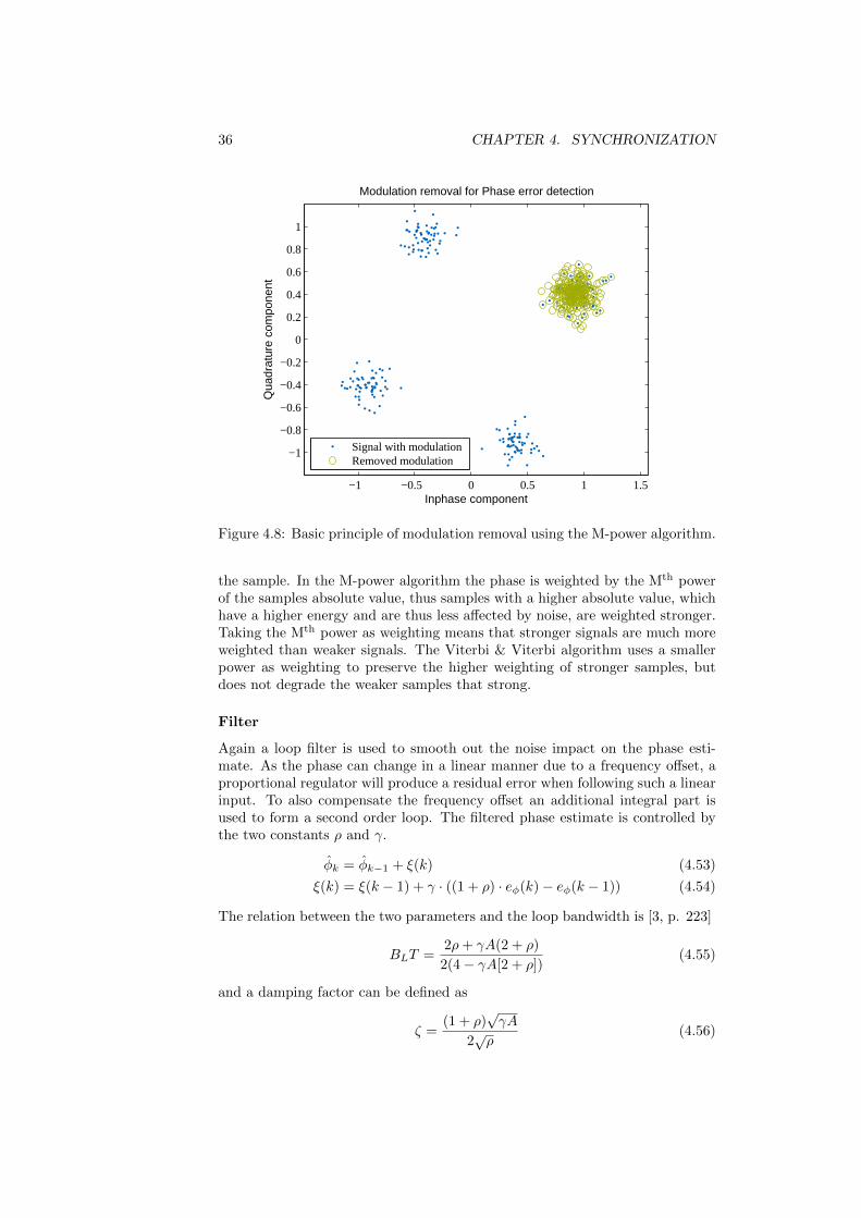
Figure 4.8 shows this effect for a QPSK (M=4) modulation. The estimatedphase is affected by noise. To generate an error signal for a tracking loop theestimated phase is usually weighted with a factor depending on the quality of


−1 −0.5 0 0.5 1 1.5

−1

−0.8

−0.6

−0.4

−0.2

0

0.2

0.4

0.6

0.8

1

Modulation removal for Phase error detection

Inphase component

Qua

drat

ure

com

pone

nt

Signal with modulationRemoved modulation

Figure 4.8: Basic principle of modulation removal using the M-power algorithm.

the sample. In the M-power algorithm the phase is weighted by the Mth powerof the samples absolute value, thus samples with a higher absolute value, whichhave a higher energy and are thus less affected by noise, are weighted stronger.Taking the Mth power as weighting means that stronger signals are much moreweighted than weaker signals. The Viterbi & Viterbi algorithm uses a smallerpower as weighting to preserve the higher weighting of stronger samples, butdoes not degrade the weaker samples that strong.

Filter

Again a loop filter is used to smooth out the noise impact on the phase esti-mate. As the phase can change in a linear manner due to a frequency offset, aproportional regulator will produce a residual error when following such a linearinput. To also compensate the frequency offset an additional integral part isused to form a second order loop. The filtered phase estimate is controlled bythe two constants ρ and γ.

φk = φk−1 + ξ(k) (4.53)

ξ(k) = ξ(k − 1) + γ · ((1 + ρ) · eφ(k)− eφ(k − 1)) (4.54)

The relation between the two parameters and the loop bandwidth is [3, p. 223]

BLT =2ρ+ γA(2 + ρ)

2(4− γA[2 + ρ])(4.55)

and a damping factor can be defined as

ζ =(1 + ρ)

√γA

2√ρ

(4.56)

4.3. TRACKING 37

The slope of the S-curve at the origin is one and a damping factor ζ = 1√2

is chosen. Choosing BLT from the observation length L of the feedforwardestimator and using equation (4.49) the two equations can be solved for the twounknown parameters γ and ρ.

4.3.3 Simulation Results

To ensure the proper function of the tracking a generated sample sequence withknown phase offset and delay is generated and tracked. The resulting errorbetween estimated and real parameter as well as the corresponding error signalsfrom Sections 4.3.1 and 4.3.2 for a noise free case are plotted in Figure 4.9a onthe following page and with noise in Figure 4.9b.

4.3.4 Measured Results

The results from tracking the initially synchronized samples from Section 4.2.5on page 31 are shown in Figure 4.10 on page 39. It can be seen that the alreadywell synchronized samples from Figure 4.10a are rotated even a bit more to theoriginal BPSK symbols, but are almost untouched. In comparison the initiallysynchronized samples from Figure 4.10b are as well concentrated around thetwo BPSK symbols by the tracking loop and a detection is now possible. As thetracking operates on single samples the number of samples does not affect theaccuracy of the estimation and even for much longer sequences the separationbetween the M-PSK samples will be possible.


500 1000 1500 2000 2500 3000−5

0

5x 10

−3∆τ

500 1000 1500 2000 2500 3000−0.5

0

0.5

eτ

500 1000 1500 2000 2500 3000−0.01

0

0.01

∆φ[rad]

500 1000 1500 2000 2500 3000−0.01

0

0.01

eφ[rad]

(a) without noise

500 1000 1500 2000 2500 3000−0.05

0

0.05

∆τ

500 1000 1500 2000 2500 3000−2

0

2

eτ

500 1000 1500 2000 2500 3000−0.02

0

0.02

∆φ[rad]

500 1000 1500 2000 2500 3000−0.2

0

0.2

eφ[rad]

(b) with noise (σ2 = 0.0316 ⇔ SNR = 15dB)

Figure 4.9: Simulated tracking results

4.3. TRACKING 39

−1 −0.8 −0.6 −0.4 −0.2 0 0.2 0.4 0.6 0.8 1

−0.6

−0.4

−0.2

0

0.2

0.4

0.6


Qua

drat

ure

com

pone

nt [1

00 ]

Signal constellation of tracked and decimated samples

Samples [104]1 2 3 4 5 6

initially synchronized samplestracked samples

(a) Short sequence of samples

−1 −0.8 −0.6 −0.4 −0.2 0 0.2 0.4 0.6 0.8 1

−0.6

−0.4

−0.2

0

0.2

0.4

0.6


Qua

drat

ure

com

pone

nt [1

00 ]

Signal constellation of tracked and decimated samples

Samples [105]1 2 3 4 5 6

initially synchronized samplestracked samples

(b) Large sequence of Samples

Figure 4.10: Measured tracking results compared to the initially synchronizedsamples


4.4 Start of Frame Detection

After the successful bit synchronization of the previous sections there are stilltwo open points. Because of the π-ambiguity of the phase of the BPSK syn-chronization sequence it is unclear whether a received +1 corresponds to a oneor a zero and it has to be detected which bit is the first bit that belongs tothe send data. These two issues can be resolved by sending a known start offrame sequence and correlate the received bits with this sequence. A Barkersequence of length 13 is used as start of frame sequence either directly or theKronecker product of two barker sequences to get a sequence of length 132 forhigher robustness. Barker sequences have an autocorrelation function with aoff-peak autocorrelation of at most one. The maximum crosscorrelation of thesynchronization sequence with the 13 bit Barker code is five, while the autocor-relation of two aligned Barker sequences is 13. The received samples are BPSK

0 50 100 150 200 250 300 350 400 450−1

−0.8

−0.6

−0.4

−0.2

0

0.2

0.4

0.6

0.8

1

Offset

Nor

mal

ized

Cor

rela

tion

Start of Frame detection for SNR=5dB

Figure 4.11: Simulated correlation between the demodulated samples and thestart of frame sequence

demodulated by taking the real value of them and are then correlated with azero padded start of frame sequence. Figure 4.11 shows the normalized corre-lation of such a sequence. A clear and distinctive peak can be observed at anoffset of 250. In this case the correlation at the detected maximum is negative,so the received samples have to be rotated by π before detection, otherwise thesamples are already aligned.

4.5 Data Transmission over the USRPs

Finally all the thoughts from this Chapter should be used to transmit data overthe USRPs. First the vector of transmission symbols is generated starting with

4.5. DATA TRANSMISSION OVER THE USRPS 41

the synchronization sequence from Section 4.2, followed by the start of framesequence of Section 4.4 and a M-PSK modulated random data sequence. Thesesymbols are filtered with a root-raised cosine filter and are transmitted over anUSRP.

The received samples are checked for the presence of a synchronization se-quence as described in Section 4.2.4 and the frequency and phase offsets aswell as the delay of the received samples from the synchronization sequence areestimated by the feedforward estimator of Section 4.2.1 at the middle of thesynchronization sequence.

The samples starting at the middle of the synchronization sequence arerotated by the estimated phase and frequency offset and are filtered with amatched root raised cosine filter. These filtered samples are then tracked anddecimated.

A fixed number of the corrected and decimated samples of the tracking loopare then send to the BPSK detector to search for the start of frame and resolvethe phase ambiguity, as described in Section 4.4. All symbols that belong tothe data sequence are then M-PSK demodulated taking the detected phaseambiguity into account. The demodulated data sequence is then compared tothe generated data sequence to see if any bit errors have occurred.

43

Chapter 5

Summary

In the first part of this work a fully functional interface between MATLABand the USRPs has been developed. With this interface it is now possible toaccess the USRP devices, set all necessary parameters and transmit and receivesamples with or without time tagging even from multiple USRPs as long as theMATLAB Thread is fast enough to catch up with the data rates.

In the second part a synchronization scheme was investigated to be usedfor frequency, timing and phase synchronization of USRP transmissions. It hasbeen shown in simulations that the used feedforward estimator achieves theCramer-Rao bounds. It has also been shown that the used tracking algorithmsare capable of keeping the M-PSK symbols separable over long durations ofrandom transmitted data. Afterwards the start of frame sequence has beenused to align the bit synchronized data stream and resolve the phase ambiguityof the received samples. Finally the received samples have been demodulatedand detected both in simulations as well as with measured data from the USRPs,using the interface of the first part of this work.

Based on these two parts it is now possible to use a coherent USRP chan-nel in MATLAB for further testing of communication schemes where existingsimulation MATLAB code can be reused and without having to worry aboutsynchronization.

45

Appendix A

A.1 Send and Receive Multiple Data Streamsfrom a Single Thread

Listing A.1: Sample code to send and transmit from one single Thread

1 #include <uhd/usrp/multi_usrp.hpp >

2 #include <stdio.h>

3 #include <string >

4 #include <complex >

5 #include <unistd.h>

6

7 int main(void){

8 // desired data rate in samples per seconds

9 double datarate = 2000000.0; // 2 Msamples per second

10 // desired center frequency

11 double frequency = 1490000000.0; // 1.49 GHz

12 // maximum time for read our buffer , before return

13 double timeout = 0.008; // 8 ms

14

15 // how many samples should be read out at once

16 const size_t max_samps_per_packet = 25000;

17 // number of read/write cycles that should be done

18 const int num_packets = 10000;

19

20 // counting variables

21 size_t i;

22 size_t rx_num , tx_num;

23

24 // default device

25 std:: string args("");

26 uhd::usrp:: multi_usrp ::sptr usrp = uhd::usrp:: multi_usrp ::

make(args);

27

28 // set datarates

29 usrp ->set_rx_rate(datarate);

30 usrp ->set_tx_rate(datarate);

31

32 // set center frequencys

33 usrp ->set_rx_freq(frequency);

46 APPENDIX A. APPENDIX

34 usrp ->set_tx_freq(frequency);

35

36 // no amplification needed

37 usrp ->set_rx_gain (0.0);

38 usrp ->set_tx_gain (0.0);

39

40 // space to store metadata

41 uhd:: rx_metadata_t rx_md;

42 uhd:: tx_metadata_t tx_md;

43 uhd:: async_metadata_t async_md;

44

45 // send as soon as possible (no time tagging)

46 tx_md.has_time_spec = false;

47

48 // buffers for sending and receiving

49 std::vector <std::complex <double > > rx_buff(

max_samps_per_packet);

50 std::vector <std::complex <double > > tx_buff(

max_samps_per_packet);

51

52 // create send signal inside the buffer

53 for(i=0;i<max_samps_per_packet;i++) {

54 // create complex cosine (alternating +/ -1+0i)

55 tx_buff[i] = std::complex <double >(((i%2 == 0) ? -1 : 1),

0);

56 }

57

58 // start streaming

59 printf("start streaming\n");

60 usrp ->issue_stream_cmd(uhd:: stream_cmd_t ::

STREAM_MODE_START_CONTINUOUS);

61

62 for(i=num_packets ;i>0 ;i--) {

63 // send out the whole buffer

64 tx_num = usrp ->get_device ()->send(& tx_buff.front (),

tx_buff.size(), tx_md , uhd:: io_type_t :: COMPLEX_FLOAT64 ,

uhd:: device :: SEND_MODE_FULL_BUFF);

65

66 // receive until the buffer is full , or timeout seconds

went by

67 rx_num = usrp ->get_device ()->recv(& rx_buff.front (),

rx_buff.size(), rx_md , uhd:: io_type_t :: COMPLEX_FLOAT64 ,

uhd:: device :: RECV_MODE_FULL_BUFF , timeout);

68

69 // receive asynchronous messages (errors during

transmission) with 1ms timeout

70 if (usrp ->get_device ()->recv_async_msg(async_md , 0.001) &&

async_md.event_code != uhd:: async_metadata_t ::

EVENT_CODE_BURST_ACK) {

71 // metadata was not an acknowledgement , every other

metadata packet signals transmission problems

72 printf("tx error\n");

73 }

74

A.2. SEND AND RECEIVE SAMPLES TO A FILE 47

75 // if received less samples than transmitted , print out

the numbers

76 if(rx_num < max_samps_per_packet) {

77 printf("send: %d, recv: %d, max:%d\n" ,(int)tx_num , (int)

rx_num , (int)max_samps_per_packet);

78 }

79

80 // when there are receive errors , print them out

81 if(rx_md.error_code != uhd:: rx_metadata_t :: ERROR_CODE_NONE

) {

82 printf("rx error\n");

83 }

84

85 // sleep some time to simulate data processing in MATLAB

86 usleep (5000);

87 }

88

89 // signal the USRP to stop transmitting

90 tx_md.end_of_burst = true;

91 usrp ->get_device ()->send("", 0, tx_md , uhd:: io_type_t ::

COMPLEX_FLOAT64 , uhd:: device :: SEND_MODE_FULL_BUFF);

92

93 // stop receiving

94 usrp ->issue_stream_cmd(uhd:: stream_cmd_t ::

STREAM_MODE_STOP_CONTINUOUS);

95

96 printf("finished\n");

97 return 0;

98 }

A.2 Send and Receive Samples to a File

A.2.1 Sending Samples

Listing A.2: Sample code to read out samples from a file and transmit themover the USRP

1 // The following code is based on the rx_samples_to_file

example from the UHD library code

2 #include <uhd/utils/thread_priority.hpp >

3 #include <uhd/utils/safe_main.hpp >


5 #include <iostream >

6 #include <fstream >

7 #include <csignal >


9

10 // prepare the function to abort reception later on

11 static bool stop_signal_called = false;

12 void sig_int_handler(int){stop_signal_called = true;}

13

14 // programm entry point


15 int UHD_SAFE_MAIN(int argc , char *argv []){

16 // print help message when lacking parameters

17 if(not (argc == 7 || argc == 6)) {

18 printf("usage: %s usrpargs filename frequency rate gain

[numsamps ]\n", argv [0]);

19 return 1;

20 }

21

22 // give the uhd threads their desired priorities

23 uhd:: set_thread_priority_safe ();

24

25 // parse input parameters

26 const std:: string args(argv [1]);

27 const std:: string file(argv [2]);

28 const double freq = atof(argv [3]);

29 const double rate = atof(argv [4]);

30 const double gain = atof(argv [5]);

31 const size_t samps_total = (argc == 7) ? strtoul(argv[6],

NULL , 10) : 0;

32

33 // number of samples to receive before writing them into a

file

34 const size_t samps_per_buff = samps_total; // first

receive all samples and then write the file

35 // number of samples to read from the UHD in each loop

cycle

36 const size_t samps_per_loop = 10000; // 10 thousand

37



40

41 // create the USRP device


make(args);

43

44 // set transmission rate , frequency and gain

45 usrp ->set_rx_rate(rate);

46 usrp ->set_rx_freq(freq);

47 usrp ->set_rx_gain(gain);

48

49 // if no fixed number of samples is given , let the user

abbort the reception

50 if (samps_total == 0){

51 std:: signal(SIGINT , &sig_int_handler);

52 printf("Press Ctrl + C to stop streaming ...\n");

53 }

54

55 // create a receive streamer

56 uhd:: stream_args_t stream_args(std:: string("fc64"));

57 uhd:: rx_streamer ::sptr rx_stream = usrp ->get_rx_stream(

stream_args);

58

59 // store metadata

60 uhd:: rx_metadata_t md;


61

62 // allocate the buffer

63 std::vector <std::complex <double > > buff(samps_per_buff);

64

65 // create the file stream

66 std:: ofstream outfile ((file.c_str()), std:: ofstream ::

binary);

67

68 // counter of the overall received samples

69 size_t rx_total =0;

70

71 printf("Start recording :\n");

72

73 //setup streaming

74 uhd:: stream_cmd_t stream_cmd(

75 (samps_total == 0) ?

76 uhd:: stream_cmd_t :: STREAM_MODE_START_CONTINUOUS :

77 uhd:: stream_cmd_t :: STREAM_MODE_NUM_SAMPS_AND_DONE

78 );

79 stream_cmd.num_samps = samps_total;

80 stream_cmd.stream_now = true;

81 usrp ->issue_stream_cmd(stream_cmd);

82

83 // mail loop

84 while(not stop_signal_called && rx_total <samps_total){

85 // counter of received samples in this loop

86 size_t i = 0;

87 while(i<samps_per_buff) {

88 size_t num_rx_samps = rx_stream ->recv(&buff.at(i),

samps_per_loop , md);

89 i += num_rx_samps;

90

91 // show progress

92 std::cout << ".";

93 flush(std::cout);

94

95

96 if (md.error_code == uhd:: rx_metadata_t ::

ERROR_CODE_TIMEOUT) {

97 printf("rx timeout\n");

98 }


ERROR_CODE_OVERFLOW){

100 printf("rx_error\n");

101 }

102 if (md.error_code != uhd:: rx_metadata_t ::

ERROR_CODE_NONE){

103 printf("Unexpected error code 0x%x", md.error_code);

104 }

105 }

106 // write buffer to file

107 outfile.write(( const char*)&buff.front(), i*sizeof(std::

complex <double >));

108 // increase the overall counter


109 rx_total += i;

110 }

111 // close file

112 outfile.close();

113

114 printf("\n\nDone!\n");

115 return 0;

116 }

Listing A.3: Sample code to write sample data into a file

1 function writesamples(data , filename , varargin)

2 % writesamples - Write samples into a file and transmit them

over the USRP

3 % Syntax: writesamples(data , filename , [usrp_arg , freq ,

rate , gain])

4 % Input: data - Vector of 1xN samples

5 % filename - The name and path of the file to

store the samples

6 % usrp_arg - The device argument for the USRP

7 % freq - Center frequency of the USRP

8 % rate - Sampling rate of the USRP

9 % gain - Receive gain of the USRP

10

11 if(~( isempty(varargin) || length(varargin) == 4))

12 % wrong number of input variables

13 error(’usage: writesamples(data , filename , [usrp_arg ,

freq , rate , gain])’);

14 end

15 % write sequential double values as alternating real and

imaginary part

16 tmp = zeros (2* length(data (:)), 1);

17 tmp (1:2: end) = real(data (:));

18 tmp (2:2: end) = imag(data (:));

19 % clear original data sequence

20 clear data;

21 % open the samples file

22 fid = fopen(filename , ’w’);

23 %write data

24 fwrite(fid , tmp , ’double ’);

25 %close file and clean up temporary variables

26 fclose(fid);

27 clear tmp fid;

28

29 if(length(varargin) == 4)

30 % all parameters are given , receive befor reading the

file

31 usrp_arg = varargin {1};

32 freq = varargin {2};

33 rate = varargin {3};

34 gain = varargin {4};

35 % execute the transmit script from within matlab

36 command = sprintf(’./ tx_samples_from_file %s %s %f %f %f

’,usrp_arg ,filename , freq , rate , gain);


37 system(command);

38 end

39 end

A.2.2 Receiving Samples

Listing A.4: Sample code to receive samples from the USRP and store them ina file

1 // The following code is based on the rx_samples_to_file

example from the UHD library code

2 #include <uhd/utils/thread_priority.hpp >

3 #include <uhd/utils/safe_main.hpp >


5 #include <iostream >

6 #include <fstream >

7 #include <csignal >


9

10 // prepare the function to abort reception later on

11 static bool stop_signal_called = false;

12 void sig_int_handler(int){stop_signal_called = true;}

13

14 // programm entry point

15 int UHD_SAFE_MAIN(int argc , char *argv []){

16 // print help message when lacking parameters

17 if(not (argc == 7 || argc == 6)) {

18 printf("usage: %s usrpargs filename frequency rate gain

[numsamps ]\n", argv [0]);

19 return 1;

20 }

21



24

25 // parse input parameters

26 const std:: string args(argv [1]);

27 const std:: string file(argv [2]);

28 const double freq = atof(argv [3]);

29 const double rate = atof(argv [4]);

30 const double gain = atof(argv [5]);

31 const size_t samps_total = (argc == 7) ? strtoul(argv[6],

NULL , 10) : 0;

32

33 // number of samples to receive before writing them into a

file

34 const size_t samps_per_buff = samps_total; // first

receive all samples and then write the file

35 // number of samples to read from the UHD in each loop

cycle

36 const size_t samps_per_loop = 10000; // 10 thousand

37




40

41 // create the USRP device


make(args);

43

44 // set transmission rate , frequency and gain

45 usrp ->set_rx_rate(rate);

46 usrp ->set_rx_freq(freq);

47 usrp ->set_rx_gain(gain);

48

49 // if no fixed number of samples is given , let the user

abbort the reception

50 if (samps_total == 0){

51 std:: signal(SIGINT , &sig_int_handler);

52 printf("Press Ctrl + C to stop streaming ...\n");

53 }

54

55 // create a receive streamer

56 uhd:: stream_args_t stream_args(std:: string("fc64"));

57 uhd:: rx_streamer ::sptr rx_stream = usrp ->get_rx_stream(

stream_args);

58

59 // store metadata

60 uhd:: rx_metadata_t md;

61

62 // allocate the buffer

63 std::vector <std::complex <double > > buff(samps_per_buff);

64

65 // create the file stream

66 std:: ofstream outfile ((file.c_str()), std:: ofstream ::

binary);

67

68 // counter of the overall received samples

69 size_t rx_total =0;

70

71 printf("Start recording :\n");

72

73 // setup streaming

74 uhd:: stream_cmd_t stream_cmd(

75 (samps_total == 0) ?

76 uhd:: stream_cmd_t :: STREAM_MODE_START_CONTINUOUS :

77 uhd:: stream_cmd_t :: STREAM_MODE_NUM_SAMPS_AND_DONE

78 );

79 stream_cmd.num_samps = samps_total;

80 stream_cmd.stream_now = true;

81 usrp ->issue_stream_cmd(stream_cmd);

82

83 // mail loop

84 while(not stop_signal_called && rx_total <samps_total){

85 // counter of received samples in this loop

86 size_t i = 0;

87 while(i<samps_per_buff) {


88 size_t num_rx_samps = rx_stream ->recv(&buff.at(i),

samps_per_loop , md);

89 i += num_rx_samps;

90

91 // show progress

92 std::cout << ".";

93 flush(std::cout);

94

95


ERROR_CODE_TIMEOUT) {

97 printf("rx timeout\n");

98 }


ERROR_CODE_OVERFLOW){

100 printf("rx_error\n");

101 }

102 if (md.error_code != uhd:: rx_metadata_t ::

ERROR_CODE_NONE){

103 printf("Unexpected error code 0x%x", md.error_code);

104 }

105 }

106 // write buffer to file

107 outfile.write(( const char*)&buff.front(), i*sizeof(std::

complex <double >));

108 // increase the overall counter

109 rx_total += i;

110 }

111 // close file

112 outfile.close();

113

114 printf("\n\nDone !\n");

115 return 0;

116 }

Listing A.5: Sample code to read out a file with raw sample data

1 function data = readsamples(filename , offset , varargin)

2 % readsamples - Receive samples from the USRP into a file

and read them out

3 % Syntax: data = readsamples(filename , offset , [usrp_arg

, freq , rate , gain , numsamps ])

4 % Input: filename - The name and path of the file to

store the samples

5 % offset - Number of samples at the beginning

to ignore

6 % usrp_arg - The device argument for the USRP

7 % freq - Center frequency of the USRP

8 % rate - Sampling rate of the USRP

9 % gain - Receive gain of the USRP

10 % numsamps - Number of samples to receive

11 % Output: data - Vector or 1xN samples with

12 % N = numsamps if provided

13


14 if(length(varargin) == 5)

15 % all parameters are given , receive befor reading the

file

16 usrp_arg = varargin {1};

17 freq = varargin {2};

18 rate = varargin {3};

19 gain = varargin {4};

20 numsamps = varargin {5};

21 % execute the receive script from within matlab

22 command = sprintf(’./ rx_samples_to_file %s %s %f %f %f %

d’,usrp_arg ,filename , freq , rate , gain , numsamps+

offset);

23 system(command);

24 elseif (~ isempty(varargin))

25 % wrong number of input variables

26 error(’usage: data = readsamples(filename , [usrp_arg ,

freq , rate , gain , numsamps ])’);

27 end

28 % open the samples file

29 fid = fopen(filename);

30 % read sequential double values and store them as doubles

31 tmp=fread(fid , ’*double ’);

32 % odd data are the real values and even data the imaginary

values of the samples

33 data=complex(tmp ((2* offset +1) :2: length(tmp)),tmp ((2* offset

+2):2: length(tmp)));

34 %close file

35 fclose(fid);

36 end

A.3 Send and Receive Samples from MATLAB

Listing A.6: Sample code to send and receive samples over the Mex interfacefrom within MATLAB.

1 % choose USRP devices

2 uhdsend = uhdinterface(’init’,’serial =4 e2610f4 ’);

3 uhdrecv = uhdinterface(’init’,’addr =192.168.10.2 ’);

4

5 % set parameters

6 uhdinterface(uhdsend ,’set_tx_freq ’ ,1.5e9)

7 uhdinterface(uhdsend ,’set_tx_rate ’,1e6)

8 uhdinterface(uhdsend ,’set_tx_gain ’ ,10)

9 uhdinterface(uhdrecv ,’set_rx_freq ’ ,1.5e9)

10 uhdinterface(uhdrecv ,’set_rx_rate ’,1e6)

11 uhdinterface(uhdrecv ,’set_rx_gain ’ ,30)

12

13 % get messages from the UHD lib

14 uhdinterface(’flush’);

15

16 % number of samples to receive/transmitt per loop

17 buf_len = 50000;

A.4. SPECTRUM ANALYZER 55

18

19 % number of loop cycles

20 n = 50;

21

22 % generate send signal (constant carrier) and preassign

receive buffer

23 send_buf = ones(buf_len ,1) *(1+0j);

24 recvvec = zeros(buf_len*n,1);

25

26 % start receiving and streaming

27 uhdinterface(uhdrecv ,’rx_stream_start ’)

28 uhdinterface(uhdsend ,’tx_stream_start ’)

29 uhdinterface(uhdsend ,’send’,send_buf);

30

31 % throw away the first samples (which already include the

transmit signal)

32 recvvec (:,1) = uhdinterface(uhdrecv ,’receiven ’,buf_len);

33

34 % send and rceive loop

35 for i=1:n

36 uhdinterface(uhdsend ,’send’,send_buf);

37 recvvec ((i-1)*buf_len +1:i*buf_len) = uhdinterface(

uhdrecv ,’receiven ’,buf_len);

38 end

39

40 % stop streaming

41 uhdinterface(uhdsend ,’tx_stream_stop ’);

42 uhdinterface(uhdrecv ,’rx_stream_stop ’);

43

44 % close USRP and unlock mexfile

45 uhdinterface(uhdsend ,’close’)

46 uhdinterface(uhdrecv ,’close’)

A.4 Spectrum Analyzer

Listing A.7: Sample code to use the USRP interface as a spectrum analyzer inMATLAB.

1 clear all;

2 close all;

3

4 % choose USRP device

5 % uhd = uhdinterface(’init ’,’serial =4e2610f4 ’); %USRP1

6 uhd = uhdinterface(’init’,’serial =4 e2611ca ’); %USRP1

7 % uhd = uhdinterface(’init ’,’addr =192.168.10.2 ’); %USRP N210

8

9 % data rate in samples per second

10 rate = 0.5e6;

11 % freq = 1541.6 e6; % Inmarsat 4F2

12 % freq = 1878.5 e6; % Meteosat 9

13 freq = 2e9;

14 gain = 20;


15 update_time = 0.1;

16 avrg_len = 10;

17

18 % setparameters

19 uhdinterface(uhd ,’set_rx_freq ’,freq)

20 uhdinterface(uhd ,’set_rx_rate ’,rate)

21 uhdinterface(uhd ,’set_rx_gain ’,gain)

22

23 % get messages from the UHD lib

24 uhdinterface(’flush’);

25

26 %length of buffer

27 N = 10e3;

28

29 % number of loop cycles to skip before recomputing the fft

30 n = ceil(update_time/N*rate);

31

32 % frequency vector

33 f = (((0:N-1) - ceil(N/2)) / N * rate) + freq;

34 % generate axis label

35 figurehandle = figure (1);

36 % set(figurehandle , ’Windowstyle ’, ’modal ’);

37 plothandle = plot(f,zeros(size(f)));

38 xlabel(’Frequency [Hz]’);

39 y_max = 0;

40 y_min = -150;

41 x_max = max(f);

42 x_min = min(f);

43 axis([x_min x_max y_min y_max ]);

44

45 % start receiving

46 uhdinterface(uhd ,’rx_stream_start ’);

47

48 % throw away the first N samples

49 vec = uhdinterface(uhd ,’receiven ’,N);

50

51 i = 1;

52 reset_avrg = true;

53 % receive wave form

54 while true

55 vec = uhdinterface(uhd ,’receiven ’,N);

56 if not(ishandle(plothandle))

57 break;

58 end

59 if(i >= n)

60 i = 1;

61 newfftvec = 20* log10(abs(fftshift(fft(vec))/N));

62 if reset_avrg

63 fftvec = newfftvec;

64 reset_avrg = false;

65 else

66 fftvec = (avrg_len*fftvec + newfftvec)/( avrg_len

+1);

67 end

A.5. AVAILABLE INTERFACE COMMANDS 57

68 set(plothandle ,’YData’,fftvec); % Update the plot

line

69 drawnow;

70 end

71

72 % pressedKey = get(figurehandle , ’CurrentCharacter ’);

73 % if pressedKey == ’q’

74 % break;

75 % end

76 i = i+1;

77 end

78

79 % stop streaming

80 uhdinterface(uhd , ’rx_stream_stop ’);

81

82 % close USRP and unlock mexfile

83 uhdinterface(uhd , ’close’);

84

85 % set(figurehandle , ’Windowstyle ’, ’normal ’);

A.5 Available Interface Commands

The interface calls have the following form

[return] = uhdinterface([index], command, [parameter]);

where a value enclosed in brackets [] is an optional value. If an index is possiblebut none is supplied the default USRP with index 0 is used. The possiblecommands are:

init returns USRP index, no index, optional string parameterInitializes a USRP object with the given device argument, or an emptystring if no argument is supplied. The USRP object is created and stored.The index to this USRP object is returned as positive (or zero) integervalue. If the returned value is negative there has been an error and noUSRP object has been created.

flush returns nothing, no index, no parameterPrints out new messages from the UHD on the MATLAB console, doesnothing if there are no new messages.

set rx freq offset returns nothing, optional index, scalar double parameterChanges the receiving centre frequency offset of the selected USRP objectto the provided frequency offset in Hz. This option offsets the operationalfrequency of the A/D converters and is afterwards compensated by theUSRP’s DSP. This offset is useful when transmitting and receiving at thesame frequency on the same daughterboard to prevent crosstalk of the RXand TX path.

set rx freq returns nothing, optional index, scalar double parameterChanges the receiving centre frequency of the selected USRP object to theprovided frequency in Hz.


set rx rate returns nothing, optional index, scalar double parameterChanges the receiving sampling rate of the selected USRP object to theprovided sampling rate in samples per second.

set rx bw returns nothing, optional index, scalar double parameterChanges the receiving channel filter of the selected USRP object to theprovided bandwidth in Hz if this operation is supported by the daughter-board.

set rx gain returns nothing, optional index, scalar double parameterChanges the receiving amplification gain of the selected USRP object tothe provided gain in the range from 0 to 30.

set rx subdev returns nothing, optional index, string parameterChanges the RX subdevice to the specified one.

set rx antenna returns nothing, optional index, string parameterChanges the RX antenna to the specified one.

receiven returns vector of complex samples, optional index, scalar integer pa-rameterTries to receive the provided amount of samples from the selected USRP.All received samples are returned in an Nx1 vector where N is either thenumber of requested samples or less, if a timeout occurred during recep-tion.

set tx freq returns nothing, optional index, scalar double parameterChanges the sending centre frequency of the selected USRP object to theprovided frequency in Hz.

set tx rate returns nothing, optional index, scalar double parameterChanges the sending sampling rate of the selected USRP object to theprovided sampling rate in samples per second.

set tx bw returns nothing, optional index, scalar double parameterChanges the sending channel filter of the selected USRP object to theprovided bandwidth in Hz if this operation is supported by the daughter-board.

set tx gain returns nothing, optional index, scalar double parameterChanges the sending amplification gain of the selected USRP object tothe provided gain in the range from 0 to 30.

set tx subdev returns nothing, optional index, string parameterChanges the TX subdevice to the specified one.

set tx antenna returns nothing, optional index, string parameterChanges the TX antenna to the specified one.

set tx timespec returns nothing, optional index, scalar double parameterSets the absolute time of transmission of the next data package (initializedby the next send command) in seconds.

A.5. AVAILABLE INTERFACE COMMANDS 59

send returns integer number, optional index, vector of complex doubles as pa-rameterTries to send the provided samples from the selected USRP. Returns thenumber of send samples which is either the number of provided samplesor less, if a timeout occurred during transmission.

get rx freq returns scalar double, optional index, no parameterReturns the receiving centre frequency of the selected USRP in Hz.

get rx rate returns scalar double, optional index, no parameterReturns the receiving sampling rate of the selected USRP in samples persecond.

get rx bw returns scalar double, optional index, no parameterReturns the receiving channel filter bandwidth of the selected USRP inHz if this operation is supported by the daughterboard..

get rx gain returns scalar double, optional index, no parameterReturns the receiving amplification gain of the selected USRP in the rangefrom 0 to 30.

get rx subdev returns string, optional index, no parameterReturns the pretty print string of the RX subdevice.

get rx antenna returns string, optional index, no parameterReturns the pretty print string of the RX antenna.

get rx timespec returns scalar double, optional index, no parameterReturns the absolute timespec of the last received packet (initialized bythe previous receiveN command) in seconds.

rx stream start returns nothing, optional index, no parameterStarts the reception of samples into the internal buffer of the selectedUSRP.

rx stream stop returns nothing, optional index, no parameterStops the reception of samples into the internal buffer of the selectedUSRP.

get tx freq returns scalar double, optional index, no parameterReturns the sending centre frequency of the selected USRP in Hz.

get tx rate returns scalar double, optional index, no parameterReturns the sending sampling rate of the selected USRP in samples persecond.

get tx bw returns scalar double, optional index, no parameterReturns the sending channel filter bandwidth of the selected USRP in Hzif this operation is supported by the daughterboard..

get tx gain returns scalar double, optional index, no parameterReturns the sending amplification gain of the selected USRP in the rangefrom 0 to 30.


get tx subdev returns string, optional index, no parameterReturns the pretty print string of the TX subdevice.

get tx antenna returns string, optional index, no parameterReturns the pretty print string of the TX antenna.

tx stream start returns nothing, optional index, no parameterStarts the transmission of samples from the internal buffer of the selectedUSRP with a delay of 1ms.

tx stream stop returns nothing, optional index, no parameterStops the transmission of samples from the internal buffer of the selectedUSRP.

close returns nothing, optional index, no parameterCloses the selected USRP object and if no other USRP object is left, theMex function is unlocked.

closeAll returns nothing, no index, no parameterCloses all USRP objects and the Mex function is unlocked.

test returns optional scalar double, no index, optional scalar double parameterIf a parameter is given an internal test variable is assigned with the valueof the parameter. If a return value is requested the current value of thetest variable is returned.

A.6 Derivation of the Maximum Likelihood Es-timator

The equality of

2L−1∑k=0

cos2(π

[k

2− τ])

= L (A.6.1)

should be shown, as used in Section 4.2.1 on page 25

2L−1∑k=0

cos2(π

[k

2− τ])

=

2L−1∑k=0

1

2

(1 + cos

(2π

[k

2− τ]))

=

2L−1∑k=0

1

2

(1 + (−1)

kcos (2πτ)

)=

2L−1∑k=0

1

2+ cos (2πτ) ·

2L−1∑k=0

(−1)k

︸︷︷︸=0

=L. �

A.6. DERIVATION OF THE MAXIMUM LIKELIHOOD ESTIMATOR 61

The equality of


}(A.6.2)

should be shown, as used in Section 4.2.1 on page 26

Γ(ν, τ) =2 |Z(ν, τ)|2

=2∣∣Ye(ν) · cos(πτ) + e−jπν · Yo(ν) · sin(πτ)

∣∣2=2 |Ye(ν)|2 · |cos(πτ)|2 + 2 |Yo(ν)|2 · |sin(πτ)|2

+ 4<{Ye(ν) · Y ∗o (ν) · ejπν · cos(πτ) · sin(πτ)

}applying addition theorems leads to:

=2 |Ye(ν)|2 · 1

2(1 + cos (2πτ)) + 2 |Yo(ν)|2 · 1

2(1− cos (2πτ))

+ 4<{Ye(ν) · Y ∗o (ν) · ejπν · 1

2sin (2πτ)

}= |Ye(ν)|2 + |Yo(ν)|2

+(|Ye(ν)|2 − |Yo(ν)|2

)cos (2πτ) + 2<

{Ye(ν)Y ∗o (ν)ejπν sin (2πτ)

}The already real valued second line can be enclosed with the < operator withoutchanging the result.

= |Ye(ν)|2 + |Yo(ν)|2 +

<

{(|Ye(ν)|2 − |Yo(ν)|2

)cos (2πτ) + 2<

{Ye(ν)Y ∗o (ν)ejπν sin (2πτ)

}}

to replace the cos and sin terms by a single complex rotation

= |Ye(ν)|2 + |Yo(ν)|2

+ <

{e2πτ

(|Ye(ν)|2 − |Yo(ν)|2 + j2<

{ejπνYe(ν)Y ∗o (ν)

})}

The inner part is defined as A(ν)

A(ν) := |Ye(ν)|2 − |Yo(ν)|2 + j2<{ejπνYe(ν)Y ∗o (ν)

}which leads to


}. �


A should be described in argument/phase notation as used in Section 4.2.1on page 26 as

|A(ν)| =∣∣Y 2e (ν) + e−j2πνY 2

o (ν)∣∣ . (A.6.3)

The squared argument of A is calculated with

|A(ν)|2 = |Ye(ν)|4 − 2 |Ye(ν)|2 |Yo(ν)|2 + |Yo(ν)|4 + 4<{ejπνYe(ν)Y ∗o (ν)

}2(A.6.4)

with <{z} = 12 (z + z∗) equation (A.6.4) becomes

|A(ν)|2 = |Ye(ν)|4 − 2 |Ye(ν)|2 |Yo(ν)|2 + |Yo(ν)|4

+ 4

(1

2

(ejπνYe(ν)Y ∗o (ν) + e−jπνY ∗e (ν)Yo(ν)

))2

= |Ye(ν)|4 − 2 |Ye(ν)|2 |Yo(ν)|2 + |Yo(ν)|4 + ej2πνY 2e (ν)Y ∗

2

o (ν)

+ 2 |Ye(ν)|2 |Y ∗o (ν)|2 + e−j2πνY ∗2

e (ν)Y 2o (ν) (A.6.5)

with z + z∗ = 2<{z} equation (A.6.5) becomes

|A(ν)|2 = |Ye(ν)|4 − 2 |Ye(ν)|2 |Yo(ν)|2 + |Yo(ν)|4

+ 2 |Ye(ν)|2 |Yo(ν)∗|2 + 2<{ej2πνY 2

e (ν)Y ∗2

o (ν)}

= |Ye(ν)|4 + |Yo(ν)|4 + 2<{ej2πνY 2

e (ν)Y ∗2

o (ν)}

=∣∣Y 2e (ν) + e−j2πνY 2

o (ν)∣∣2

which leads to

|A(ν)| =∣∣Y 2e (ν) + e−j2πνY 2

o (ν)∣∣ �

A.7 Derivation of the Likelihood of HypothesisTwo

The likelihood of hypothesis two, as used in Section 4.2.4 on page 31 is

ΨH2 = maxν

{∣∣∣∣∣2L−1∑k=0

r[k] · e−jπνk∣∣∣∣∣− L

2

}(A.7.1)

A.7. DERIVATION OF THE LIKELIHOOD OF HYPOTHESIS TWO 63

which can be calculated with

ψH2 =−2L−1∑k=0

∣∣∣r[k]− ej(πν(k−L)+φ) · 1∣∣∣2

=−2L−1∑k=0

(|r[k]|2 − 2<

{r[k] · e−j(πν(k−L)+φ)

})− 2L

ΨH2 =

2L−1∑k=0

<{r[k] · e−j(πν(k−L)+φ)

}− L

2

=<

{ej(πνL−φ) ·

2L−1∑k=0

r[k] · e−jπνk}− L

2(A.7.2)

The optimal value for πνL− φ will rotate the sum onto the real-axis.

φ− πνL =− ]

{2L−1∑k=0

r[k] · e−jπνk}

φ =− ]

{2L−1∑k=0

r[k] · e−jπνk}

+ πνL (A.7.3)

Inserting this optimal phase into (A.7.2)

ΨH2 =

∣∣∣∣∣2L−1∑k=0

r[k] · e−jπνk∣∣∣∣∣− L

2

The maximum likelihood of this hypothesis can then be achieved by taking themaximum over all frequencies ν

ΨH2 = maxν

{∣∣∣∣∣2L−1∑k=0

r[k] · e−jπνk∣∣∣∣∣− L

2

}�

BIBLIOGRAPHY 65

Bibliography

[1] M. Morelli and A. D’Amico, “Maximum Likelihood Timing and CarrierSynchronization in Burst-Mode Satellite Transmissions,” EURASIP Journalon Wireless Communications and Networking, 2007.

[2] F. Gardner, “A BPSK/QPSK Timing-Error Detector for Sampled Re-ceivers,” IEEE Transactions on Communications, May 1986.

[3] U. Mengali and A. D’Andrea, Synchronization Techniques for Digital Re-ceivers. Plenum Press, 1997.

[4] A. J. Viterbi and A. Viterbi, “Nonlinear Estimation of PSK-Modulated Car-rier Phase with Application to Burst Digital Transmission,” IEEE Transac-tions on Information Theory, July 1983.

[5] F. A. Hamza. (2011) The USRP under 1.5X Magnifying Lens! [Online].Available: http://gnuradio.org/redmine/attachments/download/129

[6] Ettus Research. (2012) UHD Wiki. [Online]. Available: http://code.ettus.com/redmine/ettus/projects/uhd/wiki

[7] Karlsruhe Institute of Technology Communications Engineering Lab. (2011)Simulink-USRP: Universal Software Radio Peripheral (USRP) Blockset.[Online]. Available: http://www.cel.kit.edu/english/downloads.php

[8] MathWorks. (2011) MATLAB and Simulink Support Package for USRP c©

Hardware. [Online]. Available: http://www.mathworks.de/discovery/sdr/usrp.html

[9] Q. Funke, “Implementation of an ECSS Compliant Ground Station Us-ing Software Defined Radios,” Diploma Thesis, Technische UniversitatMunchen, July 2012.

http://gnuradio.org/redmine/attachments/download/129

http://code.ettus.com/redmine/ettus/projects/uhd/wiki

http://code.ettus.com/redmine/ettus/projects/uhd/wiki

http://www.cel.kit.edu/english/downloads.php

http://www.mathworks.de/discovery/sdr/usrp.html

http://www.mathworks.de/discovery/sdr/usrp.html

evaluation of synchronization algorithms with usrp€¦ · evaluation of synchronization algorithms...

Documents