evaluation of the light emission kinetics in luciferin

EVALUATION OF THE LIGHT EMISSION KINETICS IN LUCIFERIN/LUCIFERASE-

BASED IN VIVO BIOLUMINESCENCE IMAGING FOR GUIDANCE IN THE

DEVELOPMENT OF SMALL ANIMAL IMAGING STUDY DESIGN

APPROVED BY SUPERVISORY COMMITTEE

Ralph P. Mason, Ph.D., CSci., C.Chem. (Mentor) Peter P. Antich, Ph.D., D. Sc. (Chairman) Joseph Gilio, Ph.D. Edmond Richer, Ph.D. Dawen Zhao, M.D., Ph.D.

DEDICATION

I dedicate this dissertation to my wife, Twila, whose unrequited support, partnership

and love has carried me every second, minute, hour, day and year on the path of this

adventure. There are not enough words of appreciation that can be expressed.

I also dedicate this work to my children, Robert and Courtney, and their spouses, Sara

and Jeff, all of whom I love and am incredibly proud of, for their continual encouragement

and forbearance, and to my grandchildren, who have given up their quality time so that

“Grumps” could pursue a passion.

I finally dedicate this effort to my parents, Bill and Peggy Bollinger, for having

encouraged me towards science, giving me the freedom of independence, and for being role

models for success through perseverance and hard work.

I want to thank the members of my Graduate Committee for their time and effort in

supporting me in completion of this project. I first thank my department chairman, and the

chairman of my committee, Dr. Antich, for his ever continuing encouragement not to be

satisfied with searching for answers to the small questions, but for maintenance of a vision

for solutions to larger and more important problems. I also thank him for his quiet (yet

ii

noticed and very appreciated), professional and mentoring care that he provided to this very

non-traditional, and at times non-cooperative, student and for his wide-ranging knowledge

and wisdom which he imparted in his own unique manner. His never-ending quest in the

research and development of the latest in imaging technologies made possible my studies in

this field.

I want to thank Dr. Mason, my mentor, who encouraged and supported me in moving

forward with this particular line of research in bioluminescent imaging. His allowance of a

controlled freedom, with his seemingly never-ending collaborations, made it possible to

pursue exciting research (limited only by my available time) in biomedical areas from basic

molecular sciences to cancer research to myocardial repair mechanisms. His never-say-die

attitude and continual pursuit of opportunities for the members of his laboratory are

inspirational.

I must also thank Dr. Edmond Richer, a fine engineer, for his support and extensive

knowledge in the ground-breaking work at UTSWMC in use of the CCD camera for

biomedical imaging. I only attained what I may have by standing on his shoulders.

Thanks are also due to Dr. Zhao who mentored me in some of the fine art of animal

surgery skills, assisted me in tissue staining, and answered my most basic questions in the

biological sciences.

I also want to thank all of the collaborators with whom I have worked, for giving me

the opportunity to learn from the wisdom of their extremely varied experiences. I especially

value the friendships of the investigators in the Division of Radiological Sciences from

iii

around the globe (including the United States, Russia, Romania, China, and India) for

making this an immensely enjoyable and very worthwhile investment in time.

I want to thank the other students for the special fellowship over the past several

years, in particular Lan Jiang, Celeste Roney, Gang Ren and Todd Soesbe as well as those

who have already achieved their PhDs and are making their individual marks on the world,

including Matthew Lewis and Vince Bourke. I pray a blessing on each of you.

Finally, when asked why I was attending graduate school at this late time in life, I

responded, “God told me to.” I hope that I have served well at UTSW. If so, it was in no

small measure due to the continual prayer, friendship, and support of the department

administrator, Kay Emerson. THANKS.

iv




by

ROBERT ALBIN BOLLINGER

DISSERTATION

Presented to the Faculty of the Graduate School of Biomedical Sciences

The University of Texas Southwestern Medical Center at Dallas

In Partial Fulfillment of the Requirements

For the Degree of

DOCTOR OF PHILOSOPHY

The University of Texas Southwestern Medical Center at Dallas

Dallas, Texas

April 2006

Copyright

by

Robert Albin Bollinger 2006

All Rights Reserved




Publication No.

Robert Albin Bollinger, Ph.D.

The University of Texas Southwestern Medical Center at Dallas, April 2006

Supervising Professor: Ralph P. Mason, Ph.D., CSci., C.Chem.

Bioluminescence imaging (BLI) is gaining acceptance as a small animal imaging modality

useful for visualizing cellular and molecular activity in vivo, and especially for evaluating

tumor development and efficacies of treatments. Various studies have validated the

technique for a number of purposes, including the quantification of tumor burden; however,

many basic questions have not been investigated whose answers may ultimately impact the

conclusions drawn from the results. Primarily, consideration of the impact of BLI emission

kinetics has not been rigorously addressed. This study provides information on the effects of

vii

different routes of luciferin substrate injection on the BLI kinetic profile, including time to

peak emission, magnitude of peak emission, and emission decay characteristics. This study

also presents for the first time the use of subcutaneous (s.c.) luciferin injection and the use of

s.c. luciferin injection followed by continuous s.c. infusion (s.c.i.) for establishment of stable

BLI light emission. Further, results are presented of the kinetic profile changes associated

with 1) inhaled and injected anesthesia; and 2) ambient air heating on mouse core

temperature. The study demonstrated substantial differences in the peak light emission with i.v.

providing the highest, with s.c., s.c.i. and i.p yielding 30% or less of the light emission of the i.v.

route. The correlations between tumor burden and BLI light emission were moderately strong

(R>0.75) for each administration route, but at varying times following injection, providing

information for establishment of optimal image start times. Surprisingly, ambient cooling of the

animal while under anesthesia yielded peak light emissions of up to 100% higher than those obtained

when ambient air heating was used to maintain mouse core temperature. Finally, guidelines are

presented to aid investigators in development of BLI study design to give due consideration

to luciferin administration routes, anesthesia protocol, and animal temperature maintenance.

viii

TABLE OF CONTENTS

PRIOR PUBLICATION ..................................................................................................... xiii

LIST OF FIGURES ............................................................................................................. xiv

LIST OF TABLES ............................................................................................................ xxiii

LIST OF APPENDICES ................................................................................................... xxiv

CHAPTER 1 - INTRODUCTION AND BACKGROUND .................................................. 1

1.1 Luciferin/Luciferase Bioluminescence Reaction ....................................................... 1

1.2 Tissue Optics .............................................................................................................. 5

1.3 Bioluminescence Imaging ........................................................................................ 12

1.3.1 CCD Camera Hardware in Bioluminescence Imaging ................................... 12

1.3.2 Software Tools in Bioluminescence Imaging ................................................. 21

1.3.3 Luciferin Biodistribution ................................................................................ 22

1.3.4 Luciferin Toxicity ........................................................................................... 22

1.4 Animal Use and Care ............................................................................................... 23

1.5 Statistical Analysis ................................................................................................... 23

CHAPTER 2 - BIOLUMINESCENCE IMAGING TO FOLLOW IN VIVO CELL

GROWTH ............................................................................................................................ 24

2.1 Initial In Vivo Small Animal Bioluminescence Imaging Studies ............................ 24

2.2 Initial i.p. HeLa-luc Study with the Shay/Wright Lab ............................................. 24

2.3 Cisplatin Single Time-Point Study with the Shay/Wright Lab ................................ 25

2.4 First Cisplatin and Telomerase Inhibitor Study with the Shay/Wright Lab ............ 26

2.5 Second Cisplatin and Telomerase Inhibitor Study with the Shay/Wright Lab ........ 28

ix

2.6 Summary of Study with Dr. Alan Varley ................................................................. 38

2.7 Summary of Study with Dr. Garry and Dr. Naseem ................................................ 40

CHAPTER 3 - EFFECTS OF ADMINISTRATION ROUTES ON IN VIVO

BIOLUMINESCENCE EMISSION MAGNITUDES AND KINETICS............................. 43

3.1 Background .............................................................................................................. 43

3.2 Initial Light Emission Kinetics of i.p. HeLa-luc Cells and Their Subsequent Tumor

Growth in Nu/Nu Mice Following i.p. Luciferin Injection ...................................... 45

3.3 Evaluation of the Light Emission Kinetics of s.c. HeLa-luc Cells in Nu/Nu Mice

Following i.p. Luciferin Injection ............................................................................ 49


Following s.c. Luciferin Injection ............................................................................ 55


Following i.v. Luciferin Injection ............................................................................ 60


Following a Bolus s.c. Luciferin Injection Followed by a Continuous s.c. Luciferin

Infusion ..................................................................................................................... 65

3.7 Evaluation of the Light Emission Kinetics of s.c. HeLa-luc Tumors in Nu/Nu Mice

Following Intra-Tumoral (i.t.) Luciferin Injection .................................................. 71

x

3.8 Evaluation of the Light Emission Kinetics of s.c. HeLa-luc Tumors in Nu/Nu Mice

Following i.p. Luciferin Injection at a Dose Three Times Higher Than “Standard”

Dose ......................................................................................................................... 75

3.9 Conclusion - Comparison of Light Emission Kinetics from Different Routes of

Substrate Administration .......................................................................................... 78

CHAPTER 4 - CORRELATION OF IN VIVO BIOLUMINESCENCE EMISSION WITH

TUMOR SIZE ...................................................................................................................... 84

4.1 Evaluation of the s.c. Tumor In Vivo Bioluminescent Light Emission at Various Time

Points Following Luciferin i.p. Injection as Tumor Size Varies ............................. 84


Points Following Luciferin s.c. Injection as Tumor Size Varies ............................. 90


Points Following Luciferin i.v. Injection as Tumor Size Varies ............................. 94


Points Following a Bolus s.c. Luciferin Injection and a Continuous s.c. Luciferin

Infusion as Tumor Size Varies ................................................................................. 98

4.5 Conclusion - Comparison of Correlations of Light Emission with Tumor Size Based

Upon Different Routes of Substrate Administration ............................................. 102

CHAPTER 5 - EFFECTS OF ANESTHESIA ADMINISTRATION AND AMBIENT AIR

HEATING ON IN VIVO BIOLUMINESCENCE EMISSION ......................................... 106

5.1 Background ............................................................................................................ 106

xi

5.2 Evaluation of the Light Emission Kinetics of s.c. HeLa-luc Tumors in Nude/Nude

Mice Following Luciferin Injection with Differing Inhaled Anesthesia

Concentrations ....................................................................................................... 110

5.3 Conclusions Regarding Anesthesia and Ambient Air Heating .............................. 119

CHAPTER 6 – GUIDANCE ON IN VIVO BIOLUMINESCENCE IMAGING STUDY

DESIGN ............................................................................................................................. 126

6.1 Introduction ............................................................................................................ 126

6.2 Guidance on the Route of Luciferin Substrate Administration ............................. 126

6.2.1 Magnitude of Light Emission ....................................................................... 126

6.2.2 Kinetics of Light Emission ........................................................................... 127

6.2.3 Correlation Between Light Emission and Tumor Volume ........................... 127

6.2.4 Ease in Administration and Repetition of Imaging ....................................... 128

6.3 Guidance on the Use of Anesthesia ....................................................................... 130

6.4 Guidance on the Use of Ambient Air Heating ....................................................... 131

CHAPTER 7 – CONCLUSIONS ...................................................................................... 132

7.1 Bioluminescent Imaging ........................................................................................ 132

7.2 In vivo small animal fluorescence imaging ............................................................ 133

REFERENCES .................................................................................................................. 137

xii

PRIOR PUBLICATION

Zain Paroo, Robert A. Bollinger, Dwayne A. Braasch, Edmond Richer, David R. Corey,

Peter P. Antich, and Ralph P. Mason, Validating bioluminescence imaging as a high-

throughput, quantitative modality for assessing tumor burden. Mol Imaging, 2004. 3(2): p.

117-24.

xiii

LIST OF FIGURES

Figure 1.1 - Bioluminescence from D-Luciferin Oxidation Catalyzed by Firefly Luciferase 3

Figure 1.2 - Attenuation Coefficients and Selected Imaging Reporters ................................ 9

Figure 1.3 – Hemoglobin Absorption of Light Emission Shows Vasculature Above Tumor 10

Figure 1.4 – Effects of Hemoglobin on Bioluminescent Imaging ....................................... 10

Figure 1.5 - Light Transmittance Through Tissues with Different Effective Attenuation

Reporters .............................................................................................................................. 11

Figure 1.6 – 95% Intensity Depth Assuming All of the Tissue is Equally Light Emitting and

Self-Attenuating ................................................................................................................... 11

Figure 1.7 – TC 245 CCD Cookbook Camera ..................................................................... 16

Figure 1.8 – Small Animal Anesthesia System ................................................................... 16

Figure 1.9 – Spectral Response of the Kodak KAF-0402ME Used in the Genesis CCD

Camera System .................................................................................................................... 17

Figure 1.10 – Genesis CCD Camera .................................................................................... 18

Figure 1.11 – Genesis CCD Camera System and Temperature Controller ......................... 18

Figure 1.12 - Genesis CCD Camera with Fluorescence Imaging ........................................ 19

Figure 1.13 - Genesis CCD Camera with Fluorescence Excitation Sources and Filters ..... 19

Figure 1.14 – Bioluminescence Emission Spectra of D-Luciferin Oxidation Catalyzed by

Firefly Luciferase over Selected pH Ranges ....................................................................... 20

Figure 1.15 - Bioluminescence Emission Spectra Shift of Firefly Luciferase as Animal

Temperature Changes .......................................................................................................... 20

Figure 2.1 – Initial Study of BLI and Imaging of Cisplatin Efficacy .................................. 30

xiv

Figure 2.2 – Cisplatin and Telomerase Inhibitor Effect on HeLa-luc Cells Implanted i.p. . 31

Figure 2.3 - Cisplatin Control Effect on HeLa-luc Cells Implanted i.p. .............................. 32

Figure 2.4 – Cisplatin and Telomerase Inhibitor 2 Minute Integrated Light Emission ....... 33

Figure 2.5 - Cisplatin Control 2 Minute Integrated Light Emission .................................... 33

Figure 2.6 – Cisplatin and Telomerase Inhibitor Normalized to the First BLI Emission .... 34

Figure 2.7 – Cisplatin Control Normalized to the First BLI Emission ................................ 34

Figure 2.8 – Mean of Light Emission following Cisplatin and Telomerase Inhibitor

Treatment ............................................................................................................................. 35

Figure 2.9 – Mean of Light Emission following Cisplatin and Telomerase Inhibitor

Treatment (semi-log) ........................................................................................................... 35

Figure 2.10 – Mean of Normalized Light Emission following Cisplatin and Telomerase

Inhibitor Treatment .............................................................................................................. 36

Figure 2.11 – Mean of Normalized Light Emission following Cisplatin and Telomerase

Inhibitor Treatment (semi-log) ............................................................................................ 36

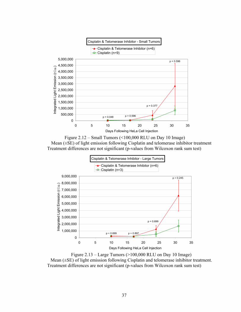
Figure 2.12 – Small Tumors Mean of Light Emission following Cisplatin and Telomerase


Figure 2.13 – Large Tumors Mean of Light Emission following Cisplatin and Telomerase


Figure 2.14 - Typical Image of ad.cmv-luc Arthritis Model in Ankle of a Rat ................... 38

Figure 2.15 - Kinetic Profile of Light Emission Following Direct Injection into Rat Ankle.39

Figure 2.16 - Typical Image of HeLa-luc Cells Growing in a Rat Gastrocnemius ............. 41

xv

Figure 2.17 - Typical Image of C2C12 Myoblast Cells with Adenovirus-luc Growing in a

Mouse Gastrocnemius .......................................................................................................... 41

Figure 2.18 - Typical Image of HeLa-luc Cells Surgically Implanted in the Myocardium . 42

Figure 3.1 – i.v. and i.p. Kinetics for One Mouse with HCT116 Colon Cancer Cells Stably

Transfected with a P53 Tumor Suppressor Gene Reporter, Pg13-luc ................................. 44

Figure 3.2 - Integrated Light Following i.p. Injection of 107 HeLa-luc Cells ..................... 46

Figure 3.3 – Representative Pseudocolor Image Following i.p. Injection of 107 HeLa-Luc

Cells .................................................................................................................................. 46

Figure 3.4 – Integrated Light Following i.p. Injection of Luciferin Cells ........................... 47

Figure 3.5 - Representative Pseudocolor Images Following i.p. Injection of Luciferin ...... 47

Figure 3.6 – Integrated Light Following I.P Luciferin Injection ......................................... 48

Figure 3.7 – Representative Pseudocolor Images Following i.p. Injection of Luciferin ..... 48

Figure 3.8 – i.p. Luciferin Injection Integrated Light Relative to the Peak of the Kinetic

Curves ................................................................................................................................. 52

Figure 3.9 – i.p. Luciferin Integrated Light Injection Relative to the Peak of the Kinetic

Curves (Semi-Log) ............................................................................................................... 52

Figure 3.10 – i.p. Luciferin Injection Integrated Light Per Volume .................................... 53

Figure 3.11 – i.p. Luciferin Injection Integrated Light Per Volume (Semi- Log) ............... 53

Figure 3.12 – i.p. Luciferin Injection Integrated Light Per Area ......................................... 54

Figure 3.13 – i.p. Luciferin Injection Integrated Light Per Area (Semi-Log) ..................... 54

Figure 3.14 – s.c. Luciferin Injection Integrated Light Relative to the Peak of the Kinetic

Curves ................................................................................................................................. 57

xvi

Figure 3.15 – s.c. Luciferin Injection Integrated Light Relative to the Peak of the Kinetic

Curves (Semi-Log) ............................................................................................................... 57

Figure 3.16 – s.c. Luciferin Injection Integrated Light Per Volume .................................... 58

Figure 3.17 – s.c. Luciferin Injection Integrated Light Per Volume (Semi- Log) ............... 58

Figure 3.18 – s.c. Luciferin Injection Integrated Light Per Area ......................................... 59

Figure 3.19 – s.c. Luciferin Injection Integrated Light Per Area (Semi-Log) ..................... 59

Figure 3.20 – i.v. Luciferin Injection Integrated Light Relative to the Peak of the Kinetic

Curves ................................................................................................................................. 62

Figure 3.21 – i.v. Luciferin Injection Integrated Light Relative to the Peak of the Kinetic

Curves (Semi-Log) ............................................................................................................... 62

Figure 3.22 – i.v. Luciferin Injection Integrated Light Per Volume .................................... 63

Figure 3.23 – i.v. Luciferin Injection Integrated Light Per Volume (Semi-Log) ................. 63

Figure 3.24 – i.v. Luciferin Injection Integrated Light Per Area ......................................... 64

Figure 3.25 – i.v. Luciferin Injection Integrated Light Per Area (Semi-Log) ..................... 64

Figure 3.26 – s.c. Bolus Injection with Continuous Infusion Integrated Light Per Volume

(n=10) .................................................................................................................................. 67


(n=10, Semi-Log) ................................................................................................................. 67

Figure 3.28 – s.c. Bolus Injection with Continuous Infusion Integrated Light Relative to the

Peak of the Kinetic Curves .................................................................................................. 68

Figure 3.29 – s.c. Bolus Injection with Continuous Infusion Integrated Light Relative to the

Peak of the Kinetic Curves (Semi- Log) ............................................................................ 68

xvii

Figure 3.30– s.c. Bolus Injection with Continuous Infusion Integrated Light Per Volume 69


(Semi-Log) ........................................................................................................................... 69

Figure 3.32– s.c. Bolus Injection with Continuous Infusion Integrated Light Per Area ..... 70

Figure 3.33 – s.c. Bolus Injection with Continuous Infusion Integrated Light Per Area

(Semi-Log) ........................................................................................................................... 70

Figure 3.34 – i.t. Luciferin Injection Integrated Light Relative to the Peak of the Kinetic

Curves ................................................................................................................................. 72

Figure 3.35 – i.t. Luciferin Injection Integrated Light Relative to the Peak of the Kinetic

Curves (Semi-Log) ............................................................................................................... 72

Figure 3.36 – i.t. Luciferin Injection Integrated Light Per Volume ..................................... 73

Figure 3.37 – i.t. Luciferin Injection Integrated Light Per Volume (Semi-Log) .................. 73

Figure 3.38 – i.v. Luciferin Injection Integrated Light Per Area.......................................... 74

Figure 3.39 – i.v. Luciferin Injection Integrated Light Per Area (Semi-Log) ..................... 74

Figure 3.40 – i.p. Luciferin Injection, at 3 Times Standard Dose, Integrated Light Per

Volume ................................................................................................................................. 77

Figure 3.41 – i.p. Luciferin Injection, at 3 Times Standard Dose, Integrated Light Per

Volume (Semi- Log) .......................................................................................................... 77

Figure 3.42 – i.v., s.c., and i.p. Light Emission Kinetic Profiles Comparison .................... 82

Figure 3.43 – i.v., s.c., and i.p. Light Emission Kinetic Profiles Comparison (Semi-Log).. 82

Figure 3.44 – Typical Imaging Sequence Overlaying Light Image, s.c. Luciferin Injection 83

xviii

Figure 4.1 – i.p. Luciferin Injection Regression Analysis of Light Emission at Peak of

Kinetic Curve Versus Volume.............................................................................................. 87

Figure 4.2 – i.p. Luciferin Injection Regression Analysis of Light Emission at 4 Minutes

Versus Volume ..................................................................................................................... 87


Versus Volume ..................................................................................................................... 88


Versus Volume ..................................................................................................................... 88


Versus Volume ..................................................................................................................... 89

Figure 4.6 – i.p. Luciferin Injection Comparison of Regression Analyses of Light Emission

Versus Volume and Area .................................................................................................. 89

Figure 4.7 – s.c. Luciferin Injection Regression Analysis of Light Emission at Peak of


Figure 4.8 – s.c. Luciferin Injection Regression Analysis of Light Emission at 4 Minutes

Versus Volume ..................................................................................................................... 91


Versus Volume ..................................................................................................................... 92


Versus Volume ..................................................................................................................... 92


Versus Volume ..................................................................................................................... 93

xix

Figure 4.12 – s.c. Luciferin Injection Comparison of Regression Analyses of Light Emission

Versus Volume and Area .................................................................................................... 93

Figure 4.13 – i.v. Luciferin Injection Regression Analysis of Light Emission at Peak of


Figure 4.14 – i.v. Luciferin Injection Regression Analysis of Light Emission at 4 Minutes

Versus Volume ..................................................................................................................... 95


Versus Volume ..................................................................................................................... 96


Versus Volume ..................................................................................................................... 96


Versus Volume ..................................................................................................................... 97

Figure 4.18 – i.v. Luciferin Injection Comparison of Regression Analyses of Light Emission

Versus Volume and Area .................................................................................................... 97

Figure 4.19 – s.c. Luciferin Bolus Injection and s.c. Luciferin Infusion Regression Analysis

of Light Emission at Peak of Kinetic Curve Versus Volume ............................................... 99

Figure 4.20– s.c. Luciferin Bolus Injection and s.c. Luciferin Infusion Regression Analysis of

Light Emission at 4 Minutes Versus Volume ...................................................................... 99

Figure 4.21– s.c. Luciferin Bolus Injection and s.c. Luciferin Infusion Regression Analysis of

Light Emission at 10 Minutes Versus Volume .................................................................. 100


of Light Emission at 22 Minutes Versus Volume .............................................................. 100

xx


of Light Emission at 40 Minutes Versus Volume .............................................................. 101

Figure 4.24 – s.c. Luciferin Bolus Injection and s.c. Luciferin Infusion Comparison of

Regression Analyses of Light Versus Volume and Area .................................................. 101

Figure 4.25 – i.p. Luciferin Injection Regression Analysis of Light Emission Versus Volume

and Relation to Absolute Rate of Change of Light Emission ............................................ 104

Figure 4.26 – s.c. Luciferin Injection Regression Analysis of Light Emission Versus Volume


Figure 4.27 – i.v. Luciferin Injection Regression Analysis of Light Emission Versus Volume


Figure 4.28 – s.c. Luciferin Injection and s.c. Infusion Regression Analysis of Light Emission

Versus Volume and Relation to Absolute Rate of Change of Light Emission .................. 105

Figure 5.1 – Representative Effect of Anesthesia on Light Emission Profile ................... 108

Figure 5.2 – Representative Effect of Anesthesia on Light Emission Profile (Semi-Log). 109

Figure 5.3 – Anesthesia and Ambient Air Heating Effects on Peak Emission .................. 115

Figure 5.4 – Kinetic Mean Light Emission Profile Using 1-1/2% Isoflurane and No Ambient

Air Heating ......................................................................................................................... 116

Figure 5.5 – Kinetic Mean Light Emission for Isoflurane and Ketamine/Xylazine, No

Ambient Air Heating .......................................................................................................... 117

Figure 5.6 – Kinetic Mean Light Emission for Isoflurane and Ketamine/Xylazine, with

Ambient Air Heating .......................................................................................................... 117

Figure 5.7 – Regression Analysis, 1-1/2% Isoflurane and No Ambient Air Heating ........ 121

xxi

Figure 5.8 – Regression Analysis, 1-1/2% Isoflurane with Ambient Air Heating ............ 121

Figure 5.9 – Regression Analysis, 2-1/2% Isoflurane and No Ambient Air Heating ........ 122

Figure 5.10 – Regression Analysis, 2-1/2% Isoflurane with Ambient Air Heating .......... 122

Figure 5.11 – Regression Analysis, Ketamine/Xylazine and No Ambient Air Heating .... 123

Figure 5.12 – Regression Analysis, Ketamine/Xylazine with Ambient Air Heating ........ 123

Figure 5.13 – Comparison of Effect of Ambient Air Heating On the R-Value of Regression

Analysis at Each Time Step, 1-1/2% Isoflurane ................................................................ 124

Figure 5.14 – Comparison of Effect of Ambient Air Heating On the R-Value of Regression

Analysis at Each Time Step, 2-1/2% Isoflurane ................................................................ 124

Figure 5.15 – Comparison of Effect of Ambient Air Heating on the R-Value of Regression

Analysis at Each Time Step, Ketamine/Xylazine .............................................................. 125

Figure 7.1 – Representative Dual Imaging of GFP-Expressing Fluorescent Cells and

Luciferase Expressing Cells ............................................................................................... 136

xxii

LIST OF TABLES

Table 3.1 – Kinetic Imaging Summary ................................................................................ 81

Table 3.2 – Summary of Peak Emission and Decay for Various Luciferin Injection Routes 81

Table 5.1 – Anesthesia and Ambient Heating Imaging Summary...................................... 113

Table 5.2 – Peak Emissions and Associated Mouse Core Temperatures .......................... 114

Table 6.1 – Guidelines for Selection of Luciferin Injection Routes .................................. 129

xxiii

LIST OF APPENDICES

Appendix A - Summary of Some of the Referenced Small Animal Bioluminescence Imaging

Studies ................................................................................................................................. 145

Appendix B – Igor Pro® Custom Procedure for Semi-Automated Generation of Images and

Integration of Light Emissions ........................................................................................... 146

xxiv

CHAPTER 1

INTRODUCTION AND BACKGROUND

1.1 Luciferin/luciferase bioluminescence reaction.

Chemiluminescence is a chemical reaction in which light of any wavelength, but

more often referring to visible light, is emitted without the coincident generation of heat.

Bioluminescence is a special case of chemiluminescence in which the chemical reaction

occurs between at least two molecules in a living biological organism. The substrate

molecule, which emits the light through an oxidative reaction, is broadly called a luciferin

(“light bearer”), and luciferase is a generic name for an enzyme, which acts as a catalyst in a

bioluminescent reaction. The reaction further may or may not require other cofactors to act

on either the luciferin or luciferase.

Luciferase and luciferin occur naturally in bacteria, fungi, dinoflagellates, radiolarians

and about 17 metazoan phyla and 700 genera with more than 30 independent origins [1], but

in all cases the light emitting reaction is not a necessity. Some organisms have only the

luciferase enzyme and require acquisition of the luciferin by ingestion. While the intent of

the reaction is not universally accepted, there is evidence that the main purpose of the

luciferin is to produce an antioxidant defense mechanism at the cellular level, optimized by

the catalyzing luciferase, with the resultant light emissions being subsequently used by the

organism for ancillary purposes including communication and prey deception [2].

There are many luciferin/luciferase bioluminescence emitting system mechanisms,

with five basic and well understood systems [3-5]: bacterial [6], dinoflagellate, coelenterate

[7], firefly [8], and Vargula. Two mechanisms are of particular interest in the subject

1

research. The first is that of the North American firefly (beetle) Photinus pyralis. The

second is that of the coelenterate jellyfish Aequorea. In the Aequorea, while the luciferase

and the substrate luciferin (known as coelenterazine) provide the bioluminescent reaction, the

accessory photoprotein, green fluorescent protein (GFP), is actually of more interest in

imaging studies [9].

Owing to its extensive use in both in vitro and in vivo applications, the mechanism

and chemical reaction of the light emission from P. pyralis have been extensively studied,

with the much of the early work performed and reported by bioluminescence pioneers

Marlene DeLuca and William McElroy at UC San Diego and Emil White and Bruce

Branchini at Johns Hopkins University. The complex reaction is understood to be a

luciferase catalyzed activation of luciferin with oxygen in the presence of cofactors with the

subsequent emission of light [8, 10-18] as shown in Figure 1.1:

Nomenclature:

D-Firefly luciferin, CAS #2591-17-5, C11H8N2O3S2 [19]

(S)-4,5-dihydro-2-(6-hydroxy-2-benzo-thiazoloyl)-4-thiazolecarboxylic acid

Luc Firefly luciferase gene: Photinus-luciferin 4-monooxygenase (ATP-

hydrolysing) – IUBMB Enzyme Nomenclature EC 1.13.12.7 [20]

ATP Adenosine triphosphate

AMP Adenosine monophosphate

2

Figure 1.1 - Bioluminescence from D-luciferin oxidation catalyzed by firefly luciferase

3

In the first step of the reaction, the substrates luciferin [Figure 1.1(a)] and cation-complexed

ATP form a ternary complex [Figure 1.1(b) - Luciferyl AMP or luciferyl adenylate] with

luciferase. Next, a proton is abstracted from the C-4 carbon of the adenylate forming an acid

anhydride with the release of pyrophosphate, then oxidized by molecular oxygen creating

highly reactive cyclic peroxide, dioxetanone [Figs. 1.1(c-d)]. Decarboxylation of the

peroxide leads to formation of oxyluciferin in a singlet electronically excited state, keto-

form, which under basic conditions (pH>7.0) rapidly transforms into the enol-form after C-5

proton removal. Upon de-excitation of the oxyluciferin to the ground state, light is emitted

[8, 13, 15].

The quantity of light emission is strongly affected by oxygen availability [21],

hypoxia [22], luciferase degradation [23], hemorrhaging [24], enzyme turnover in the

presence of luciferin [25], etc.

4

1.2 Tissue optics.

The largest drawback to bioluminescence imaging is the minimal thickness of less

than several millimeters of tissues that light from reporters penetrates before being

significantly attenuated by absorption and scattering. The problem has been widely

researched [26-33] and it is well recognized that the dominant interaction of light at optical

wavelengths is elastic scattering, described by the mean number of scatters per unit length,

µs. The scatter coefficient, µs, of many soft tissues has been measured and theoretically

calculated by many techniques, and is typically within the range of 10 – 100 mm-1 [34]. The

scattering coefficient is further refined by taking into account the asymmetry of the direction

of scatter known as the anisotropy coefficient, g, where g is the mean cosine of the single

scatter phase function. This yields a characteristic transport scatter coefficient, where µs' =

µs(1-g). For most tissues, g is about 0.7 to 0.9 and µs' is on the order of 1 mm-1. This

scattering causes blurring and is the major problem in being able to use optical light for fine

discrimination of structures and imaging of biological processes in tissues.

The second mode of interaction is the light absorption, µa, which is strongly affected

by the specific chromophores in the tissue constituents. Due to its abundance, water is the

dominant chromophore, and is strongly absorbing below 300 nm and above 1000 nm. Below

580 nm, hemoglobin is a very strong absorber and provides the largest impact on light

transmittance. At 580 nm, both oxygenated hemoglobin (HbO2) and deoxygenated

hemoglobin (Hb) light absorption fall sharply between two and three orders of magnitude

5

compared to that at 400 nm, with a relative plateau up to 950 nm, as shown in Figure 1.2

adapted from [26, 28, 35-39].

The use of fluorescent proteins and bioluminescent reporters provides the ability to

track molecular and cellular changes in vivo over a period of time with minimal or no impact

on the organism. Green fluorescent protein (GFP) is the most widely studied and used

fluorescent protein (actually an accessory protein) with a maximum emission, λmax, of 504

nm [9, 40] and has been cloned and mutated numerous times in attempts to achieve longer

wavelengths [41, 42]. These include the commercial DsRed (λmax = 583 nm) and the longest

waveshifted drFP616 (λmax = 616 nm) [43-47]. As discussed earlier, the P. pyralis luciferase

enzyme that catalyzes luciferin in the presence of ATP has a λmax of 562 nm.

As shown in Figure 1.2, the current fluorescent proteins and firefly

luciferase/luciferin have a λmax within the highly absorbing ranges of hemoglobin, although

drFP616 is on the decreasing slope of the absorption curve. In this range, the absorption of

water is 3 to 4 orders of magnitude less than the hemoglobin, but the relative amounts of each

affects the total absorption.

The effect of the absorption of light emission by hemoglobin is shown in Figure 1.3

where the vasculature between the tumor and camera is presented as a shadow image.

Further, hemoglobin can cause artifacts or confounds in quantifying tumor size based upon

light emission (discussed in Chapter 4). The 2-D BLI light image of an s.c. tumor in the

anesthesia study (discussed in Chapter 5), shows a dark, potentially necrotic area of the

tumor; however, upon removing the skin above the tumor, Figure 1.4 shows that the dark

6

area was caused by major vascular supply to the tumor. This was further confirmed by the

H&E staining (nor presents).

The depth of penetration of light through tissue is a substantial constraint and has

been researched in the applications of a number of medical fields including diagnostics,

photodynamic therapy and medical imaging [33, 48-53]. To assist in an experimental design

in collaboration with the Shay lab, a first order estimate of light transmittance was calculated

in accordance with the method presented by Tromberg et al. [54]. In non-transparent, turbid

media, consistent with most tissue, both scattering and absorption contribute to distance-

dependent light attenuation. Additionally, with multiple scattering, the light intensity

decreases according to:

zeffeII µ−= 0 Eqn. 1.1

( )[ 2/1'3 −+= saaeff µµµµ ]

)

Eqn. 1.2

( gss −= 1' µµ Eqn. 1.3 where, I0 = Initial emission intensity

I = final emission intensity

µeff = effective attenuation coefficient

µa = absorption coefficient

µs’= reduced scattering coefficient

g = angular dependence of scattering

z = depth of light source

Given the heterogeneity of the tissues that the light penetrates following emission

from an i.p. tumor, there is no single absorption coefficient, scattering coefficient, or

7

scattering angle. Further, the light from the bioluminescence or fluorescence is not emitted at

a single frequency, but rather over a narrow wavelength spectrum with a certain peak. The

absorption and scattering coefficient, as well as the scattering angle, are also dependent upon

wavelength. Therefore, no single effective attenuation coefficient is universally applicable

and µs’ varies widely. Figure 1.5 provides a graph of the effect of µeff on light transmittance,

the ratio of the light emitted from the source to that which is emitted from the tissue. If a

tissue mass is assumed to emit equal quanta of light throughout the depth, with tissue self-

attenuation the total light emitted reaches an asymptotic maximum. This can also be

displayed as shown in Figure 1.6, as the depth of tissue at which the amount of light reaches

a certain value, namely 95% in this case.

Another limitation is that the refractive index of mammalian tissue is approximately

1.4. Thus, there is a reflection of the emitted light at the tissue/air boundary of

approximately 50% [53].

8

9

GFP

Luciferin

GFP

Luciferin

Figure 1.2 – Attenuation coefficents and selected imaging reporters (Adapted fromWeissleder [35])

Figure 1.3 – Hemoglobin absorption of light emission showing vasculature above the tumor

(A) (B)

Figure 1.4 – Effects of hemoglobin on bioluminescent imaging. A) Bioluminscent light emission from a massive subcutaneous tumor with a large, dark area

of the tumor thought to be necrotic. B) Upon removing the skin from above the tumor, it was determined that the dark areas were caused by the tumor blood supply from the skin

absorbing the light emission (The animal is rotated slightly towards the top compared to the BLI image.) The tumor was determined by H&E staining to not be necrotic in the dark areas.

10

Transmittance Through Tissue

0.00

0.20

0.40

0.60

0.80

1.00

0 1 2 3 4 5 6 7 8 9 1Depth (mm)

Tran

smitt

ance

(I/I 0

)

µeff = 10/mm µeff = 5/mm µeff = 2/mm µeff = 1/mm µeff = 0.5/mm

1.0 mm

0.5125,10

0

Figure 1.5 – Light transmittance through tissues with different effective attenuation coefficients

Depth at Which of 95% Intensity Is ReachedAs a Function of Effective Attenuation Coefficient

0.01.02.03.04.05.06.07.08.09.0

10.011.012.013.014.015.0

0.0 1.0 2.0 3.0 4.0 5.0 6.0 7.0 8.0 9.0 10.0

Effective Attenuation Coefficient - µeff (mm-1)

Dep

th (m

m)

Figure 1.6 – 95% Intensity depth assuming all of the tissue is equally light emitting and self-attenuating

11

1.3 Bioluminescence imaging.

1.3.1 CCD camera hardware in bioluminescence imaging

The first generation of bioluminescence imaging system used in the Division of

Advanced Radiological Sciences is based upon the Cookbook 245 charge-coupled device

(CCD) camera, as described in The CCD Camera Cookbook [55]. The camera was built by

Dr. Shreefal Mehta, Trung Nguyen, Billy Smith and Dr. Edmond Richer in the Division of

Advanced Radiological Sciences at the University of Texas Southwestern Medical Center at

Dallas (UTSWMC). It incorporates a Texas Instruments TC245 black and white, frame

transfer CCD image sensor with an image area of 786 (H) x 488 (V) pixels, producing an

image of 252 (H) x 242 (V) pixels. The camera head consists of the CCD-chip, a two-stage

Peltier element glued to a plate, the cooling element and a heat sink. A cooling system

provides 0º C coolant to cool the CCD to –20º C to minimize the dark current. The camera is

controlled by, and the image is captured on, a personal computer for further image processing

using the CBWinCam software package (described later). Figure 1.7 shows a representative

configuration of the imaging system set up for small animal imaging. Figure 1.8 shows the

small animal anesthesia system.

In support of my research, I built a second generation optical imaging system. For

image acquisition, I assembled primarily from a kit a Genesis CCD camera, which was based

upon the French Audine astronomical camera. I selected and installed a high performance

Kodak KAF-0402ME CCD with micro-lenses for wide range image sensing in the 350nm to

1000nm range. The spectral response for this lens is shown in Figure 1.9 [56], and shows the

relatively high efficiency in the 500 to 700 nm range of interest for bioluminscent imaging.

12

This research provides the first application of this camera, CCD and software for

bioluminescence imaging. The camera is a black and white, full-frame CCD, with an image

area of 786 (H) x 512 (V) pixels, and a photoactive area of 6.91 mm x 4.6 mm. The camera

head incorporates all of the control electronics and consists of the CCD-chip, a Peltier

cooling element and heat sink (Figure 1.10) and the CCD cool is controlled by a PIC

controller with feedback from the heat sink temperature (Figure 1.11). A circulating coolant

system provided to the CCD heat sink reduces the CCD temperature to as low as –40° C,

thereby minimizing the dark current. The camera is controlled by and the image is captured

on a personal computer (Figure 1.11) for further image processing using the Pisco software

(described later). The camera was modified to allow for placement of filters within the

cameral body, and the system was supplemented with a 100W metal halide light source with

dual line light fiber optics (Dolan-Jenner Industries) for illumination during fluorescence

imaging. Excitation filters are placed in the light source to match the illumination with the

correct excitation frequency and emission filters placed in the camera to discriminate the

fluorescence of interest (Figures 1.12 and 1.13). This system has the capability to image any

optical reporter such as luciferase, GFP, dyes, or “beacons,” and can be used for in vivo and

in vitro imaging support of cellular and molecular imaging projects.

I also designed and manufactured a light-tight box for controlled conditions for

imaging and ease in modification for associated imaging applications. I also included an

LED source to allow for acquisition of “light images” of animals for overlay positioning of

the animal with the acquired images.

13

Prior to 2005, most of the literature reported bioluminescent light emission in relative

light units (r.l.u., R.L.U. or rlu) as a qualitative measure since most imaging systems used

black and white CCDs for image capture. This practice was followed in reporting the results

in this dissertation. However, an approximation can be determined for reporting the results

in photons per centimeter squared per steradian per second (ph/cm2/sr/sec). The major

limitations in conversion from rlu to ph/cm2/sr/sec are the facts that the light emission from

bioluminescence is a continuous spectrum over a range of wavelengths and that the spectrum

in vivo may have a pH dependent shift, as shown in Figure 1.14 [13], may be temperature

dependent (personal communication with Christopher Contag and [57]), and may be tissue

depth dependent [57]. Further, the efficiency of the CCD itself is wavelength dependent, as

shown in Figure 1.9. While the radiance in Watts/cm2/sr can be easily measured with a

radiometer, the conversion to ph/cm2/sr/sec is dependent upon these many factors which are

dependent upon the wavelength of the light being measured, and is not a discrete value.

While all data is reported in rlu in this dissertation, an approximation of a conversion

factor of bioluminescence light emission to ph/cm2/sr/sec for the Genesis CCD was

developed using a light box built by Dr. Edmond Richer. No conversion factor was

developed for the TC245 since it was disabled prior to Dr. Richer building the light box.

This light box had many equally-spaced light emitting diodes (LEDs) with emissions

centered at 580 nm, near the peak of the luciferase/luciferin light emission, and dual

polytetrafluoroethylene (PTFE or Teflon®) diffusion filters providing a relatively constant

radiance over the imaging area. Serial 10-second images were acquired with the Genesis

CCD system, and normalized to 1-second image imaging, providing an average of 569.2

14

(±0.4 SE) rlu/sec over the imaging area. The light box emission was also measured over the

surface of the diffuser with a National Institute of Standards and Technology (NIST)

traceable research radiometer (Model IL1700, International Light Technologies, Inc.,

Peabody, MA) which had been calibrated to display radiance in Watts/cm2/sr. The light box

provided 3.72 (±0.05 SE) x 10-4 Watts/cm2/sr. Using the energy of the light at 580 nm, the

light emission was converted to 1.08 (±0.02 SE) x 1015 ph/cm2/sr/sec. The Genesis CCD was

then cross-calibrated against the radiometer measurements, and provided a calibration factor

of 1.9 x 1012 (ph/cm2/sr/sec)/(RLU/sec), at 580 nm. To ascertain the actual radiance in

ph/cm2/sr/sec over the spectrum of the luciferin/luciferase emission requires further

knowledge of the photon energy not determinable by the existing Kodak black and white

CCD installed in the Genesis CCD Camera System.

15

Figure 1.7 – TC 245 CCD Cookbook Camera

Figure 1.8 – Small Animal Anesthesia System

16

17

Figure 1.9 – Spectral Response of the Kodak KAF-0402ME used in the Genesis CCD Camera System. The upper curve is for the KAF-0402ME. [56]

Figure 1.10 – Genesis CCD Camera

Figure 1.11 – Genesis CCD Camera System and Temperature Controller

18

Figure 1.12 – Genesis CCD Camera System with fluorescence imaging

Figure 1.13 – Genesis CCD Camera System with fluorescence excitation source and filters

19

Figure 1.14 – Bioluminescence emission spectra of D-luciferin oxidation catalyzed by

firefly luciferase over selected pH range (From Branchini et al. [13]

Figure 1.15 – Bioluminescence emission spectra shift of firefly luciferase as animal temperature changes (From Zhao et al. [57])

20

1.3.2 Software tools in bioluminescence imaging

The TC245 CCD camera is controlled by and the image is captured on a personal

computer for further image processing using the CBWinCam [58] software package. The

Genesis CCD camera is controlled by and the image is captured on a personal computer for

further image processing using the Pisco [59] software. The Pisco software is a common

package used primarily in astronomical research for the control of telescopes and acquisition

of their camera images. This study is the first known use in this application in biomedical

imaging.

All image processing is performed using the IGOR Pro, V 4.0.6.1 (Wavemetrics, Inc)

data analysis program. One of the features of IGOR Pro is the ability to develop and save

custom generated “procedures” utilizing macros and functions for repetitive image

processing. Dr. Edmond Richer developed the initial procedure to import the raw images

generated by CBWinCam in the standard Flexible Image Transport System (FITS) format

[60] used in astronomy. I substantially modified the Richer procedure to allow semi-

automatic generation of images and integration of light emissions. The modified procedure

also automatically normalizes photon emission quantity and image presentation to relative

light units per min (rlu/min) to allow for proper comparison between images independent of

image length. The procedure was modified numerous times over the timeframe of the study

to minimize manual data reduction and to provide improved display of images. A copy of

one version of the procedure used in the anesthesia study is included in Appendix A.

21

1.3.3 Luciferin biodistribution

The biodistribution of luciferin has been studied by Contag et al. by i.p. injection into

BALB/c mice and measuring the lysates of various tissues using in vitro luciferase assays.

Luciferin was found in all tissue analyzed. [61] Rehemtulla et al. have shown that luciferin

is able to cross the blood-brain barrier in studies of intracerebral tumors in male Fischer 344

rats [62] and Burgos et al. have shown the same in studies of nu/nu mice, although with the

caveat that the blood brain barrier may be the cause of differences seen in the dynamics of

bioluminescence. [63] Further, Collaco and Geusz showed general dispersal of luciferin into

the skin, internal organs, and brain, although stating that luciferin levels may not be

distributed uniformly. They concluded, however, that even low luciferin concentrations

could be saturating because the release of oxyluciferin from luciferase is rate-limiting. [64]

Lipshutz et al. have also shown transfer across the placental barrier. [65] Many other studies

have shown that luciferin is biologically well distributed [66-71]. A most comprehensive

study by Lee et al. using radiolabelled (125I) D-luciferin expressly evaluated cell uptake and

tissue distribution. [72] Lee’s results showed that luciferin is widely distributed through

blood, organs, muscle, fat and bone, although at widely different concentrations. Also, while

the blood concentration was many orders of magnitude higher than in the tissues, the intra-

cellular concentration was likely to be within the range for the reaction rate to be

significantly influenced by the luciferin concentration. Finally, Lee concluded that there

were substantial differences in biodistribution resulting from luciferin injections i.p. versus

i.v.

1.3.4 Luciferin toxicity

22

No studies have been found in the literature which evaluate the toxicity of luciferin.

While a number of studies have mentioned that the uptake of luciferin presented low toxicity

or no signs of overt toxicity [61, 67, 68, 70, 73, 74], none have explicitly evaluated luciferin

toxicity in laboratory animals. Several reports have suggested that toxicity studies should be

performed.

1.4 Animal use and care

All animal procedures were performed using bioluminescence imaging are performed

in accordance with the UTSWMC Institutional Animal Care and Use Committee guidelines.

1.5 Statistical Analyses

All statistical analyses were performed using Microsoft Excel, V. 2002 (Microsoft

Corporation, Redmond, Washington) and JMP In, V. 5.1 (SAS Institute, Inc., Cary, North

Carolina).

23

CHAPTER 2

BIOLUMINESCENCE IMAGING TO FOLLOW IN VIVO CELL GROWTH

2.1 Initial in vivo small animal bioluminescence imaging studies

The initial studies were performed in an effort to understand and refine the use of the

relatively new bioluminescence imaging hardware and techniques to follow cell growth in

small animals. Experimental protocols were developed based upon the experience gained in

the early studies with the understanding that little guidance was available from published

data, and none using this CCD camera system. Unless otherwise presented, no evaluation of

the luciferin kinetics had been performed for the initial studies, and they were executed under

the assumption that imaging at a consistent single time-point following luciferin injection,

plus or minus several minutes, would allow valid comparison of images over a long-term

study. Additionally, no study of the effects of anesthesia (either concentrations or types) had

been evaluated and the protocols were not rigorously maintained.

2.2 Initial i.p. HeLa-luc study with the Shay/Wright lab

The Jerry Shay/Woodring Wright lab at UTSWMC uses HeLa cells for research in

telomerase mechanisms and telomerase inhibition. Based upon success by other

investigators with BLI for in vivo imaging using HeLa-luc cells [22, 61, 75, 76], interest was

expressed in determining whether the CCD camera could be used to support their research.

To prove the principle, in collaboration with Dr. Meaghan Granger, four previously

irradiated Nu/Nu mice were each given one injection of HeLa-luc cells in the right flank as

follows: 105 cells i.m., 106 cells i.m., 105cells s.c. or 106 cells s.c. The mice were then

24

injected with 3 mg of luciferin in solution (15.9 mg/ml) within 4 minutes following cell

injection, anesthetized with a ketamine/xylazine cocktail within 7 minutes following cell

injection. The mice were imaged generally in accordance with the BLI imaging protocol

discussed in Section 1 with 8 minute or 30 minute integration times for the 106 and 105 cell

injections, respectively. Adequate images were obtained to allow for further experiment

design.

2.3 Cisplatin single time-point study with the Shay/Wright lab

To evaluate the ability of the BLI system to track tumor cell growth in vivo in long-

term studies and to evaluate the ability to track the efficacy of a tumor therapy, a small scale

study was performed in collaboration with Dr. Granger and the Shay/Wright. The animals (n

= 4) were injected i.p. with 106 HeLa-luc cells. On days 3, 7 and 10 following the HeLa-luc

injections, the animals were treated with Cis-platinum (II) diammine dichloride (Cisplatin), a

platinum-containing broad spectrum agent shown to be effective against various solid tumors

(Sigma-Aldrich, Inc., USA). On days 0, 3, 7, 13, 17, 20, 24, and 31 days following the

HeLa-luc injections, the animals were imaged with the CCD Cookbook camera with image

integration times between 1 minute and 16 minutes, at times following luciferin injection of

between 8 minutes and 30 minutes. The animals were sedated with 0.02 mL of Avertin per

gram of mouse weight, and maintained under anesthesia generally using 0.9% Isoflurane in 1

L/min O2. The CCD Cookbook camera was cooled by an ice bath which had to be manually

replenished. The ice bath temperature was not automatically controlled and variations would

occur that affected the dark image (noise) and, therefore, the light emission quantification.

25

The data was not quantified but the images evaluated qualitatively. While having

mixed results, the principal investigators determined that the bioluminescent imaging

technology had sufficient promise to continue with additional investigations, as shown in

Figure 2.1.

2.4 First Cisplatin and telomerase inhibitor study with the Shay/Wright lab

To further evaluate the use of bioluminscent imaging and in to support the study of

the cancer treatment efficacies, a larger study was performed in collaboration with Dr.

Granger and the Shay/Wright lab. 25 female nu/nu mice were injected i.p with HeLa-luc

cells, divided into 3 cohorts. The first group (n = 3) were controls with no treatment planned.

The second group (n = 11) was injected with Cisplatin on days 3, 7 and 10 following HeLa-

luc injection. The third group (n = 11) was treated with Cisplatin as well as 20 mg/kg of an

investigatory telomerase inhibiting drug, GRN163 (Geron Corporation, Menlo Park, CA) on

days 3, 7 and 10 following HeLa-luc injection. The animals were imaged with the CCD

Cookbook camera with 2 minute image integration times beginning 25 minutes following

luciferin injection. The animals were sedated with 0.5 mL of Avertin, and maintained under

anesthesia using 0.9% Isoflurane in 1 L/min O2. The CCD Cookbook camera was cooled by

an ice bath which had to be manually replenished. The ice bath temperature was not

automatically controlled and variations would occur that affected the dark image (noise) and,

therefore, the light emission quantification.

Of the control group, one developed tumors to provide a very minor light emission on

initial imaging on day 3. The other two did not present any light emission on day 3, and died

prior to imaging on day 10.

26

Initial imaging of the Cisplatin only group on day 3 provided 10 light emissions from

the cohort of 11. The one that did not present light emissions on day 3 did not show any

emissions until day 31. On day 10, six of the group had decreased light emissions to < 10%

of the initial images, two had emissions between 10% and 20% of initial images, and one had

emissions of 72% of initial images. The remaining animal had and increase 55% over initial

imaging. These results indicated a generally substantial reduction in tumor light emissions.

On day 17 compared to the day 10 images, three were at < 10%, one at < 26%, two increased

between 150% and 200%, two increased between 600% and 900%, one increased > 15000%,

and one died. On day 24 compared to the previous images, all emissions of live animals

increased. The results were mixed such that no strong conclusions could be drawn.

Initial imaging of the Cisplatin and telomerase inhibitor group on day 3 provided

three with no, or essentially no, light emissions from the cohort of 11. One of these never

showed emissions and one died following day 17 with no emissions. The last one began

showing emissions on day 17. On day 10, of the eight that showed emissions on the day 3

(initial imaging), six had emissions of < 5% of initial, 1 had 16% of initial, and one had 40%

of initial. These results indicated a generally substantial reduction in tumor light emissions.

On day 17 compared to the day 10 images, three had remained at zero, one < 15%, one at <

55%, one indicated light emission for the first time, one increased ~3000%, and one died.

On day 24 compared to the previous images, two remained at zero, one at < 5%, 2 increased

between 5% and 12%, and three increased between 80% and 100%. On day 31 compared to

the previous images, one decreased 36% and 5 increased between 80% and 1000%. The

results were mixed such that no strong conclusions could be drawn.

27

Based upon the results of the imaging in the first 17 days of the study, the principal

investigators determined that further testing of the BLI technology and its usefulness in

cancer treatment evaluation was warranted.

2.5 Second Cisplatin and telomerase inhibitor study with the Shay/Wright lab

A fourth HeLa-luc study was performed in collaboration with Dr. Granger and the

Shay/Wright lab to investigate a proprietary tumor treatment therapy. Two cohorts (2 x n =

12) of female nu/nu mice were injected i.p. with 106 HeLa-luc cells. On days 5, 7, and 10

following HeLa-luc injection, both cohorts were given i.p. injections of Cisplatin. The first

cohort was also injected i.p. with 20 mg/kg of the investigatory telomerase inhibitor GRN163

on days 0, 1, 2, and 3 following HeLa-luc injection, as well as 3 times per week throughout

the study.

All 24 animals were imaged for an integrated 2 minutes on days 3, 10, 17, 24 and 31

following HeLa-luc injection, starting nominally 20 minutes following luciferin injection,

using the CCD Cookbook camera. There were occasional instances when imaging time was

delayed up to 28 minutes following luciferin injection, but this time delay was assumed to be

acceptable. Figures 2.2 and 2.3 provide the complete bioluminescent image sets (with false

color for light emission intensity overlaid on a light image) for each animal in the Cisplatin

and telomerase inhibitor group and the Cisplatin control group, respectively. Figures 2.4 and

2.5 present integrated light emission for each animal over the time course of the study.

Based on previous investigations, it was known that the same number of HeLa-luc cells

injected i.p. into nu/nu mice produced highly differing tumor growth, independent of

treatments. To consider this difference, the integrated light emissions were normalized to the

28

first light emission image, and the normalized light emissions for each animal is presented in

Figures 2.6 and 2.7. The means (±SE) of the Cisplatin and telomerase inhibitor cohort and

the Cisplatin control cohort are shown in Figures 2.8 and 2.9 on a linear and semi-log scale

(for more detail), respectively. The mean for the Cisplatin and telomerase inhibitor group at

first light emission image was 157,900 (± 43,400) rlu, almost twice that of the Cisplatin

control groups mean, 85,700 (± 43,500) rlu. When evaluating the raw light emission, both

groups had a slight decrease in the mean light emission from days 10 through 17. From days

17 through 31, the light emission from both groups followed exponential growth rates, with

the Cisplatin and telomerase inhibitor group having a 2.6 day doubling time and the Cisplatin

control group having a longer 3.6 day doubling time. This appears to indicate that the group

with the telomerase inhibitor had greater tumor growth rate than the Cisplatin control group.

However, when consideration was given to normalization of the light emission to the first

BLI emission image (Figures 2.10 and 2.11), the Cisplatin and telomerase inhibitor group

had a 2.7 day doubling time compared to the Cisplatin control group having a shorter 1.9 day

doubling time. The difference in the two treatments was not shown to be significant with p-

values generally greater than 0.05 (by Wilcoxon rank sum test). The data was further

analyzed by grouping into small tumors (<100,000 rlu on day 10 imaging) and large tumors

(>100,000 rlu on day 10 imaging), and again no significant difference was found between the

two treatments (Figures 2.12 and 2.13). Nonetheless, this data provided sufficient

information to perform additional investigation of the telomerase inhibitor GRN163 as well

as other Geron compounds (not presented in this paper).

29

Day 3

Control – No Cisplatin Cisplatin Treatment (3 mg/kg) Day 7 Day 13 Day 20 Day 27 Add’l Cisplatin Day 20 (3 mg/kg)

Figure 2.1 – Initial study of BLI and imaging of Cisplatin efficacy

30

31

Days following HeLa Injection3 10 17 21 28

1

2

3

4

5

6

7

8

9

10

11

12

Mouse # RLUDays following HeLa Injection3 10 17 21 28

1

2

3

4

5

6

7

8

9

10

11

12

Mouse # RLU

Figure 2.2 – Cisplatin and telomerase inhibitor effect on HeLa-luc cells implanted i.p.

(2 min integrated light emission)

Days following HeLa Injection3 10 17 21 28

13

14

15

16

17

18

19

20

21

22

23

24

Mouse # RLUDays following HeLa Injection

3 10 17 21 28

13

14

15

16

17

18

19

20

21

22

23

24

Mouse # RLU

Figure 2.3 – Cisplatin control effect on HeLa-luc cells implanted i.p.

(2 minute integrated light emission)

32

Cisplatin & Telomerase Inhibitor

1

10

100

1,000

10,000

100,000

1,000,000

10,000,000

100,000,000

0 5 10 15 20 25 30 35Days Following HeLa Cell Injection

Inte

grat

ed L

ight

Em

issi

on (r

.l.u.

)

Telomerase Inhib. Inj. (T)Cisplatin Inj. (C)

T T T T T,C T,C T T T T T T T TC

Figure 2.4 – Cisplatin and telomerase inhibitor 2 minute integrated light emission (n = 12)

Cisplatin Control

10

100

1,000

10,000

100,000

1,000,000

10,000,000


Inte

grat

ed L

ight

Em

issi

on (r

.l.u.

)

C CCCisplatin Inj. (C)

Figure 2.5 – Cisplatin control

2 minute integrated light emission (n = 12)

33

Cisplatin & Telomerase InhibitorNormalized to First BLI Emission Image

0.001

0.010

0.100

1.000

10.000

100.000

1,000.000


Inte

grat

ed L

ight

Em

issi

on

Figure 2.6 – Cisplatin and telomerase inhibitor normalized to the first BLI emission Image (n = 12)

Cisplatin ControlNormalized to First BLI Emission Image

0.001

0.010

0.100

1.000

10.000

100.000

1,000.000

10,000.000


Inte

grat

ed L

ight

Em

issi

on

Figure 2.7 – Cisplatin control normalized to the first BLI emission image (n = 12)

34


0

1,000,000

2,000,000

3,000,000

4,000,000

5,000,000

6,000,000

7,000,000


Inte

grat

ed L

ight

Em

issi

on (r

.l.u.

)Cisplatin & Telomerase InhibitorCisplatin Control

p = 0.069

p = 0.100

p = 0.624p = 0.034

Figure 2.8 – Mean (±SE) of light emission following Cisplatin and telomerase inhibitor treatment (n = 12 each cohort)

(p-values from Wilcoxon rank sum test)


10,000

100,000

1,000,000

10,000,000


Inte

grat

ed L

ight

Em

issi

on (r

.l.u.

)

Cisplatin & Telomerase InhibitorCisplatin Control

Figure 2.9 – Mean (±SE) of light emission following Cisplatin and telomerase inhibitor treatment (n = 12 each cohort) – semi-log

35


0

200

400

600

800

1,000

1,200

1,400


Inte

grat

ed L

ight

Em

issi

on (r

.l.u.

)


Figure 2.10 - Mean (±SE) of normalized light emission following Cisplatin and telomerase inhibitor treatment (n = 12 each cohort)


0.1

1.0

10.0

100.0

1,000.0

10,000.0


Inte

grat

ed L

ight

Em

issi

on


Figure 2.11 – Mean (±SE) of normalized light emission following Cisplatin and telomerase inhibitor treatment (n = 12 each cohort) – semi-log

36

Cisplatin & Telomerase Inhibitor - Small Tumors

0

500,000

1,000,000

1,500,000

2,000,000

2,500,000

3,000,000

3,500,000

4,000,000

4,500,000

5,000,000


Inte

grat

ed L

ight

Em

issi

on (r

.l.u.

)

Cisplatin & Telomerase Inhibitor (n=6)Cisplatin (n=9)

p = 0.596

p = 0.377

p = 0.596p = 0.048

Figure 2.12 – Small Tumors (<100,000 RLU on Day 10 Image) Mean (±SE) of light emission following Cisplatin and telomerase inhibitor treatment

Treatment differences are not significant (p-values from Wilcoxon rank sum test)

Cisplatin & Telomerase Inhibitor - Large Tumors

0

1,000,000

2,000,000

3,000,000

4,000,000

5,000,000

6,000,000

7,000,000

8,000,000

9,000,000


Inte

grat

ed L

ight

Em

issi

on (r

.l.u.

)

Cisplatin & Telomerase Inhibitor (n=6)Cisplatin (n=3)

p = 0.245

p = 0.699

p = 0.897p = 0.699

Figure 2.13 – Large Tumors (>100,000 RLU on Day 10 Image) Mean (±SE) of light emission following Cisplatin and telomerase inhibitor treatment.

Treatment differences are not significant (p-values from Wilcoxon rank sum test)

37

2.6 Summary of Study with Dr. Alan Varley

Bioluminescent imaging was performed for Dr. Alan Varley with the Department of

Internal Medicine at UTSWMC for proof of principle of the ability of the BLI system to

track an arthritis model, ad.CMV-luc, in rats and to determine effectiveness of treatment.

Figure 2.14 provides a typical image following luciferin injection directly into the ankle, and

Figure 2.15 provides a kinetic image profile used to evaluate single point imaging times for a

more extensive study.

Figure 2.14 – Typical image of ad.CMV-luc arthritis model in ankle of a rat. Hair shaved to minimize light absorption (by permission of Alan Varley)

38

INTEGRATED LIGHT EMISSIONFOLLOWING INJECTION OF LUCIFERIN DIRECTLY INTO ANKLE

BACKGROUND SUBTRACTION = 5 R.L.U.

0

5,000

10,000

15,000

20,000

25,000

30,000

0 10 20 30 40 50 60 70 80 90Time After Injection of Luciferin (min.)

Ligh

t Em

issi

on (r

.l.u.

)

Figure 2.15 – Kinetic profile of light emission following direct injection into the

ankle of a rat (by permission of Alan Varley)

39

2.7 Summary of Study with Dr. Garry and Dr. Naseem

To support Drs. Daniel Garry and Rao Haris Naseem of the Department of

Cardiology, the bioluminescent imaging was evaluated for the ability to track luciferase-

transfected myoblast cells injected in the pericardium and myocardium. The first phase was

to assess the ability to detect stably-transfected HeLa-luc cells injected intramuscularly (i.m.)

in the gastocnemius. This was successfully performed as seen in Figures 2.16 and 2.17. The

next phase was to asses the ability of the imaging system to detect luciferase-transfected cells

in the myocardium. This was a concern given the depth of the tissue and the fact that it

underlies the blood-rich lungs potentially absorbing the bioluminescent light emission. As

shown in Figure 2.18, the emission was sufficient to consider imaging of cells in the heart.

The study was not completed at the time of this dissertation due to difficulty in stably

transfecting myoblast to provide a sufficient light output.

40

Figure 2.16 – Typical image of HeLa-luc cells growing in a rat gastrocnemius (by permission of Rao Haris Naseem)

Figure 2.17 – Typical image of C2C12 Myoblast Cells with adenovirus-luc growing in a mouse gastocnemius (by permission of Rao Haris Naseem)

41

42

Figure 2.18 – Typical image of HeLa-luc cells surgically implanted in the myocardium (by permission of Rao Haris Naseem)

CHAPTER 3

EFFECTS OF ADMINISTRATION ROUTES ON IN VIVO BIOLUMINESCENCE

EMISSION MAGNITUDES AND KINETICS

3.1 Background

Intraperitoneal (i.p.) injections have been the predominant route of luciferin substrate

injection for small animal imaging studies (33 of 35 studies) found in the literature [22, 25,

61-68, 72, 73, 76-97], with intravenous (i.v.) injection used in four [68, 72, 90, 98] and

transdermal also used in one of the i.p. studies [61]. Justification for the selected route of

administration was presented in only two i.p. studies due to the comparative ease in

administration [65, 90]. As discussed previously, dissimilar routes are expected to cause

different biodistributions, concentrations and clearances of the luciferin over the typical one

hour or less timeframe of most experiments. These effects are thus anticipated to influence

the magnitude and kinetics of light emissions from the luciferin/luciferase reaction, with only

the radiolabelled D-luciferin study by Lee et al. [72], and the study by Wang et al. [90]

providing one data point considering this hypothesis, as shown in Figure 3.1. Wang showed

a much higher magnitude (approximate factor of 8) for light emission from i.v. injection

compared to the i.p. injection. Further, they showed a kinetic profile with the onset of light

emission and decay of light emission both much more rapid for i.v. than for i.p. As discussed

later, the i.v. kinetics are similar to those attained in this dissertation, whereas the i.p. kinetics

appear to be inconsistent.

43

Figure 3.1 – i.v. and i.p. kinetics for one mouse with HCT116 colon cancer cells stably transfected with a p53 tumor suppressor gene reporter, PG13-Luc [90].

44

3.2 Initial light emission kinetics of i.p. HeLa-luc cells and their subsequent tumor

growth in nude/nude mice following i.p. luciferin injection

To better understand the kinetics of light emission from HeLa-luc cells in support of

the Shay/Wright telomerase studies, the first kinetic experiment was performed on August 7,

2002. Mouse “d” from the study described in Section 2.3.2 was injected i.p. with 107 HeLa-

luc cells. 28 minutes later, the mouse was sedated by i.p. injection of 0.4 ml of Avertin

(1.25% tribromoethanol), then injected i.p. with 130 µl of luciferin (D-luciferin sodium salt,

Biosynth AG), with a concentration of 17mg/ml in a TRIS buffer, pH 7.0, for a dose of 125

mg/kg. The mouse was maintained under anesthesia with a nose cone providing Isofluorane

(0.9 % with 1 l/min O2). A two minute integration image was recorded every 2 to 4 minutes

beginning 3 minutes after luciferin injection. The images were processed providing the

kinetic profile indicating cell implantation and stability as shown in Figure 3.2.

Representative pseudocolor images are shown in Figure 3.3.

To understand the kinetics of light emission from cells which have been well

established, the kinetics experiment was repeated 5 days after cell injection on mouse “d,” as

well as on mouse “b” 17 days after cell injection. The same protocol was followed, with the

exception that a delta-phase isothermal pad was placed under the mice for stabilization of

body temperature. The light emission kinetics showed a rapid increase with a peak at

approximately 20 minutes, followed by decay to background noise levels within one hour.

The light emission profile and pseudocolor images are shown in Figure 3.4 through 3.7.

These experiments provided information indicating that kinetics of the light emission should

be considered in the selection of time points in imaging protocols.

45

INTEGRATED LIGHTFOLLOWING COINCIDENT INJECTION OF 107 HeLa-Luc CELLS AND

LUCIFERIN

0

5000

10000

15000

20000

25000

30000

35000

40000

45000

0 20 40 60 80 100 1Time After Injection of Luciferin (min.)

Inte

grat

ed Im

age

(r.l.

u.)

20

Figure 3.2 – Integrated light following i.p. injection of 107 HeLa-luc cells – Mouse “d”

Figure 3.3 – Representative pseudocolor image following i.p. injection of

107 HeLa-luc cells – Mouse “d” (Times shown following i.p. injection of luciferin, 36 minutes after i.p. cell injection)

46

INTEGRATED LIGHTFOLLOWING INJECTION OF LUCIFERIN WITH A WELL ESTABLISHED TUMOR

0

200,000

400,000

600,000

800,000

1,000,000

1,200,000

0 10 20 30 40 50 60 70 8

Time After Injection of Luciferin (min.)

Inte

grat

ed Im

age

(r.l.

u.)

0

Figure 3.4 – Integrated light following i.p. injection of luciferin Mouse “d” – Day 5

Figure 3.5 – Representative pseudocolor images following i.p. injection of luciferin Mouse “d” - Day 5

47

INTEGRATED LIGHTFOLLOWING INJECTION OF LUCIFERIN WITH A WELL ESTABLISHED TUMOR

0

200,000

400,000

600,000

800,000

1,000,000

1,200,000

0 10 20 30 40 50 60 70 80 90 100

Time After Injection of Luciferin (min.)

Inte

grat

ed Im

age

(r.l.

u.)

Figure 3.6 – Integrated light following i.p. luciferin injection Mouse “b” – Day 17

Figure 3.7 – Representative pseudocolor images following i.p. luciferin injection Mouse “b” - Day 17

48

To better understand the light emission kinetics, more than 20 additional kinetic

experiments were performed on i.p. tumors generally showing a time to peak of 10 to 20

minutes, followed by a quasi-exponential decay to background levels within one hour (data

not presented). It was, however, apparent in the large number of single-time point and

kinetics experiments with over 1,100 images between August, 2002, and February, 2003, that

for intraperitoneal HeLa-luc cells with i.p. luciferin injections, the magnitude of the light

emission was highly variable. This was due in part to the nature of the tumors in the

peritoneum and movement of abdominal structures inducing the light emitting cells to change

position both laterally and, more importantly, in depth. This resulted in uncontrollable and

unpredictable effects on the light emissions through tissue attenuation, scattering and

absorption.

3.3 Evaluation of the light emission kinetics of s.c. HeLa-luc tumors in nude/nude

mice following i.p. luciferin injection

For bioluminescence imaging to meet its anticipated potential as a high throughput

technique for tracking cells in vivo, it is important that the light emissions be quantifiable.

Otherwise, the modality will provide only qualitative information with limited usefulness.

Therefore, the variables that effect the light emissions need to be characterized and the first-

order kinetic nature of bioluminescence light emissions must be considered in experimental

design to assist in valid quantification. Since i.p. cells had shown uncontrolled variability

through tissue attenuation unrelated to the cell induced bioluminescence, subcutaneous cell

tracking were expected to provide a more stable model to evaluate the kinetics.

49

In collaboration with the Dr. David Corey lab at UTSWMC, in February, 2003, Dr.

Zain Paroo provided a set (n=6) of athymic Nu/Nu mice (Harlan, Indianapolis, IN), which

had been injected subcutaneously over the left flank with 106 or 2x106 HeLa-luc cells. One

animal died early in the study and none of its data were included. As the study progressed, it

appeared that one of the tumor implantation sites was intradermal rather than subcutaneous,

so the data from this animal was also excluded leaving 4 animals. The tumors were allowed

to grow without intervention for the extent of the study (approximately one month). The

mice were injected i.p. with D-luciferin at a dose of 150 mg/kg, sedated with 3% Isofluorane

with 1 l/min O2 for 4 minutes, then maintained under anesthesia with 1% Isofluorane with 1

l/min O2. The mice were placed on a delta-phase isothermal pad for maintenance of

temperature inside the light-tight box for imaging. Two minute integration images were

taken every 3 minutes beginning 4 minutes after luciferin injection for a total of 64 minutes.

Upon completion of the kinetic imaging, while the mice were still sedated, the major axes

and height of the s.c. tumors were measured with calipers and recorded. To provide

additional statistical information, a second cohort of animals (n=6) under the same protocol

was imaged for a total of 68 kinetic imaging sequences.

Figures 3.8 and 3.9 present the relative mean (±SE) of the light emissions normalized

to the peak for each kinetic imaging set to evaluate the shape of the kinetic profile,

irrespective of emission quantity or tumor size. As shown by the small S.E., the profiles are

very similar and do not appear to be effected by either emission quantity or tumor size.

Figures 3.10 through 3.13 present the mean (±SE) of the i.p. light emissions

normalized to tumor volume (Vol 2) and tumor projected area, respectively. The decay half-

50

life of the mean emission profile immediately after peak was 11.3 min. The mean time to

peak emissions of 11.4 ± 0.4 (SE) min and the mean of the peak emissions (Vol 2) of 1,090 ±

90 (SE) rlu/min/mm3 were also calculated.

The results of the imaging study of the s.c. tumors using i.p. luciferin injections was

published by Paroo, Bollinger et al. in April 2004. [99]

51

Light Emission KineticsMean of All IP Injections (n=49)

Relative to Peak

0.000

0.100

0.200

0.300

0.400

0.500

0.600

0.700

0.800

0.900

1.000

0 5 10 15 20 25 30 35 40 45 50 55 60Time After Luciferin Injection (min)

Ligh

t Em

isss

ion

(r.l.u

./min

)

Figure 3.8 – i.p. luciferin injection Integrated light relative to the peak of the kinetic curves


Relative to Peak

0.010

0.100

1.000


Ligh

t Em

issi

on (r

.l.u.

/min

)

Figure 3.9 – i.p. luciferin injection Integrated light relative to the peak of the kinetic curves (semi-log)

Exponential decay: t1/2=11.6 min (16-34 min); t1/2=19.6 min (40-64min)

52


Integrated Light per Volume (W2*L/2)

0

200

400

600

800

1,000

1,200


Ligh

t Em

issi

on (r

.l.u.

/min

/mm

3 )

Figure 3.10 – i.p. luciferin injection Integrated light per volume



10

100

1,000

10,000


Ligh

t Em

issi

on (r

.l.u.

/min

/mm

3 )

Figure 3.11 – i.p. luciferin injection Integrated light per volume (semi-log)

Exponential decay: t1/2=11.3 min (16-34 min); t1/2=19.4 min (36-55 min)

53

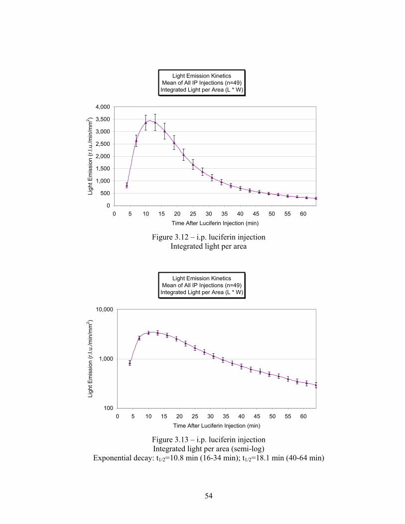
Light Emission KineticsMean of All IP Injections (n=49)Integrated Light per Area (L * W)

0

500

1,000

1,500

2,000

2,500

3,000

3,500

4,000


Ligh

t Em

issi

on (r

.l.u.

/min

/mm

2 )

Figure 3.12 – i.p. luciferin injection Integrated light per area

Light Emission KineticsMean of All IP Injections (n=49)Integrated Light per Area (L * W)

100

1,000

10,000


Ligh

t Em

issi

on (r

.l.u.

/min

/mm

2 )

Figure 3.13 – i.p. luciferin injection Integrated light per area (semi-log)


54


mice following s.c. luciferin injection

During the s.c. tumor kinetic studies, approximately 10% of the i.p. injections in the

first cohort of animals provided minimal or no light emission when tumors were present and

in which light emissions were obtained prior to or afterwards, or both. This offered the

possibility that luciferin i.p. injections could be somewhat problematic in that the injections

may have hit abdominal organs and limited the luciferin absorption through the peritoneal

tissues for distribution via the vasculature to the tumor sites. This could create an

unnecessary confound if little or no light emission is obtained when imaging bioluminescent

cells in a location otherwise inaccessible for secondary verification, the cell locations most

aided by the non-invasive BLI technique. To overcome this potentiality, subcutaneous

injection as an alternative injection route was hypothesized to minimize potential

misadministration. As discussed in the background, only i.p. and i.v. have been published as

luciferin administration routes, and there has been no discussion of the possible benefits or

drawbacks to s.c. administration.

In parallel with the second i.p. injection cohort (n=6 mice, n=49 injection) and to

allow for a direct comparison, s.c. injection of luciferin following the same protocol for

kinetic imaging was performed in the same animals (n=27 injections). The injections were in

the s.c. space on the foreback of the mice allowing the injection bolus to be easily and

visually ascertained to minimize misadministration. Of the 27 kinetic imaging experiments,

none presented indication of unacceptable injection. As in the i.p and s.c. injections, tumor

sizes were recorded immediately following imaging while the mice were still sedated.

55

Figures 3.14 and 3.15 present the relative mean (±SE) of the light emissions

normalized to the peak for each kinetic imaging set to evaluate the shape of the kinetic

profile, irrespective of emission quantity or tumor size. As shown by the small S.E., the

profiles are very similar and do not appear to be effected by either emission quantity or tumor

size.

Figures 3.16 through 3.19 present the mean (±SE) of the s.c. light emissions


life of the mean emission profile immediately after peak was 6.2 ± 0.1 (SE) min. The mean

time to peak emissions of 11.1 ± 0.3 (SE) min and the mean of the peak emissions (Vol 2) of

1,890 ± 210 (SE) rlu/min/mm3 were also calculated.

56

Light Emission KineticsMean of All SC Luciferin Injections (n=27)

Relative to Peak

0.000

0.100

0.200

0.300

0.400

0.500

0.600

0.700

0.800

0.900

1.000


Ligh

t Em

issi

on (r

.l.u.

/min

)

Figure 3.14 – s.c. luciferin injection Integrated light relative to the peak of the kinetic curves


Relative to Peak

0.010

0.100

1.000


Ligh

t Em

issi

on (r

.l.u.

/min

)

Figure 3.15 – s.c. luciferin injection Integrated light relative to the peak of the kinetic curves (semi-log)

Exponential decay: t1/2=6.8 min (16-34 min); t1/2=10.6 min (40-53min)

57



0

500

1,000

1,500

2,000

2,500


Ligh

t Em

issi

on (r

.l.u.

/min

/mm

3 )

Figure 3.16 – s.c. luciferin injection Integrated light per volume



10

100

1,000

10,000


Ligh

t Em

issi

on (r

.l.u.

/min

/mm

3 )

Figure 3.17 – s.c. luciferin injection Integrated light per volume (semi-log)


58


Integrated Light per Area (L x W)

0

1,000

2,000

3,000

4,000

5,000

6,000

7,000

8,000


Ligh

t Em

issi

on (r

.l.u.

/min

/mm

2 )

Figure 3.18 – s.c. luciferin injection Integrated light per area



100

1,000

10,000


Ligh

t Em

issi

on (r

.l.u.

/min

/mm

2 )

Figure 3.19 – s.c. luciferin injection Integrated light per area (semi-log)


59


mice following i.v. luciferin administration

When the kinetic studies were being performed, intravenous (i.v.) luciferin injections

had been reported in only three of the sample studies [68, 72, 90]. Since this route provides

luciferin directly into the circulatory system, then to the tumor cell vasculature without the

intermediate absorption through peritoneal tissues or dermal tissue, it was hypothesized that

the i.v. injections would provide a more rapid bioluminescence emission. Following

completion of this study, this hypothesis was partially confirmed by Lee et al. [72] by use of

radioiodine-labeled D-luciferin in a biodistribution study (as discussed in detail in Section

1.3.5), although no bioluminescence data was obtained.

In parallel with the second i.p. injection cohort and the s.c. injection cohort (n=6

mice), and to allow for a direct comparison, i.v. injections of luciferin following the same

protocol for kinetic imaging were performed in the same animals (n=19 injections)

interspersed in time with the other injections. Only ten successful injections were obtained

out of 19 attempts, due primarily to inexperience with and difficulty of the i.v. technique.

Tumor sizes were again recorded immediately following imaging, while the mice were still

sedated. As necessary to prevent saturation of the CCD pixels due to the higher

bioluminescence emission rate following i.v. injection, the image integration time and time

between images were reduced to as short as 15 second images every 30 seconds, over a total

of 64 minutes. To allow direct comparison, all i.v. kinetic study data were reduced and

recalculated, and are presented in 2 minute integrations every 3 minutes as in the i.p. and s.c.

studies.

60

Figures 3.20 and 3.21 present the relative mean (±SE) of the light emissions

normalized to the peak for each kinetic imaging set to evaluate the shape of the kinetic

profile, irrespective of emission quantity or tumor size. As shown by the small S.E., the

profiles are very similar and do not appear to be effected by either emission quantity or tumor

size.

Figures 3.22 through 3.25 present the mean (±SE) of the s.c. light emissions


life of the mean emission profile immediately after peak was 3.6 ± 0.5 (SE) min. The mean

time to peak emissions of 5.2 ± 0.5 (SE) min and the mean of the peak emissions (Vol 2) of

6,040 ± 1,130 (SE) rlu/min/mm3 were also calculated.

61

Light Emission KineticsMean of All IV Injections (n=10)

Relative to Peak

0.000

0.100

0.200

0.300

0.400

0.500

0.600

0.700

0.800

0.900

1.000


Ligh

t Em

issi

on (r

.l.u.

/min

)

Figure 3.20 – i.v. luciferin injection Integrated light relative to the peak of the kinetic curves


Relative to Peak

0.001

0.010

0.100

1.000


Ligh

t Em

issi

on (r

.l.u.

/min

)

Figure 3.21 – i.v. luciferin injection Integrated light relative to the peak of the kinetic curves (semi-log)


62



0

1,000

2,000

3,000

4,000

5,000

6,000

7,000

8,000


Ligh

t Em

issi

on (r

.l.u.

/min

/mm

3 )

Figure 3.22 – i.v. luciferin injection Integrated light per volume



10

100

1,000

10,000


Ligh

t Em

issi

on (r

.l.u.

/min

/mm

3 )

Figure 3.23 – i.v. luciferin injection Integrated light per volume (semi-log)

Exponential decay: t1/2=3.6 min (19-28 min); t1/2=5.6 min (31-40 min); t1/2=8.4 min (40-49 min)

63

Relative Light Signal KineticsMean of All IV Injections (n=10)


0

5,000

10,000

15,000

20,000

25,000

30,000

35,000


Rel

ativ

e Li

ght S

igna

l (r.l

.u./m

in/m

m2 )

Figure 3.24 – i.v. luciferin injection Integrated light per area

Relative Light Signal KineticsMean of All IV Injections (n=10)


10

100

1,000

10,000

100,000


Rel

ativ

e Li

ght S

igna

l (r.l

.u./m

in/m

m2 )

Figure 3.25 – i.v. luciferin injection Integrated light per area (semi-log)

Exponential decay: t1/2=3.7 min (19-28 min); t1/2=5.6 min (31-40 min); t1/2=8.7 min (40-49 min)

64


mice following a bolus s.c. luciferin injection followed by a continuous s.c. luciferin

infusion

The kinetic nature of the i.p., i.v, and s.c. luciferin injection routes provides a

potential problem in performing bioluminescence imaging studies where quantitative

information is required. To minimize this confound, it was hypothesized that the light

emissions could be stabilized by a standard bolus injection of luciferin, followed by a

continuous infusion of luciferin to offset the normal degradation or clearance of the luciferin

from the circulatory system. Given the ease of administration of the s.c. injection route, a

series of experiments was planned to test this procedure.

In parallel with the second i.p. injection cohort and the s.c. and i.v. injection cohort

(n=6 mice), and to allow for a direct comparison, s.c. bolus injections of luciferin followed

by a subcutaneous infusion following the same protocol for kinetic imaging were performed

in the same animals (n=10 injections) interspersed in time with the other injections. The

mice were injected subcutaneously with the bolus injection in the foreback, then placed in the

light-tight box on the delta-phase heating pad, and anesthetized with isoflurane. A custom

manufactured infusion set with a 30 ga needle was inserted subcutaneously into the foreback

near the location of the bolus injection. This infusion set was pre-filled with luciferin and

connected to a 1 ml syringe filled with luciferin and installed in a syringe pump. The syringe

pump had been pre-calibrated and appropriate settings made for this syringe type to infuse at

approximately 10 µl/min. Upon initiation of integration of the first image at 4 minutes post-

65

bolus injection, the syringe pump was started, and the start quantity of luciferin in the syringe

recorded. Although 10 µl/min was expected, the actual rate was approximately 11.7 µl/min.

Additionally, the tumor sizes were recorded as in previous injection route protocols.

As shown in Figures 3.26 and 3.27, eight of the ten kinetic profiles for light emission

per volume showed relatively stable light emission. Figures 3.28 and 3.29 present the

relative mean (± SE) of the light emissions normalized to the peak for each kinetic imaging

set to evaluate the shape of the kinetic profile, irrespective of emission quantity or tumor

size.

Figures 3.30 through 3.33 present the mean (± SE) of the i.p. light emissions


life of the mean emission profile immediately after peak was 11.3 min. The mean time to

peak emissions was not calculated since the intent was not to achieve a peak, and would have

been meaningless. As shown in the Figure 3.26, some profiles continued to increase

throughout the imaging. Likewise, the decay half-life was not calculated. The mean of the

peak emissions (Vol 2) of 1,660 ± 170 (SE) rlu/min/mm3 was also calculated.

66

Light Emission KineticsSC Luciferin Injections @ Time = 0 Minutes (n=10)

SC Infusion of Luciferin @ 11.5 µL/MinMean Integrated Light per Volume (W2*L/2)

0

1,000

2,000

3,000

4,000

5,000

6,000


Ligh

t Em

issi

on (r

.l.u.

/min

/mm

3 )

Figure 3.26 – s.c. bolus luciferin injection with 11.5 µl/min continuous infusion at t=4 min Integrated light per volume



100

1,000

10,000


Ligh

t Em

issi

on (r

.l.u.

/min

/mm

3 )

Figure 3.27 - s.c. bolus luciferin injection with 11.5 µl/min continuous infusion at t=4 min Integrated light per volume (semi-log)

67

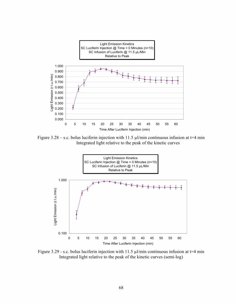
Light Emission KineticsSC Luciferin Injection @ Time = 0 Minutes (n=10)

SC Infusion of Luciferin @ 11.5 µL/MinRelative to Peak

0.0000.1000.2000.3000.4000.5000.6000.7000.8000.9001.000


Ligh

t Em

issi

on (r

.l.u.

/min

)

Figure 3.28 – s.c. bolus luciferin injection with 11.5 µl/min continuous infusion at t=4 min Integrated light relative to the peak of the kinetic curves


SC Infusion of Luciferin @ 11.5 µL/MinRelative to Peak

0.100

1.000


Ligh

t Em

issi

on (r

.l.u.

/min

)

Figure 3.29 - s.c. bolus luciferin injection with 11.5 µl/min continuous infusion at t=4 min Integrated light relative to the peak of the kinetic curves (semi-log)

68


SC Infusion of Luciferin @ 11.5 µL/MinIntegrated Light per Volume (W2*L/2)

0

500

1,000

1,500

2,000

2,500


Ligh

t Em

issi

on (r

.l.u.

/min

/mm

3 )

Figure 3.30 –s.c. bolus luciferin injection with 11.5 µl/min continuous infusion at t=4 min Integrated light per volume



100

1,000

10,000


Ligh

t Em

issi

on (r

.l.u.

/min

/mm

3 )

Figure 3.31 –s.c. bolus luciferin injection with 11.5 µl/min continuous infusion at t=4 min Integrated light per volume (semi-log)

69


SC Infusion of Luciferin @ 11.5 µL/MinMean Integrated Light per Area (L x W)

01,0002,0003,0004,0005,0006,0007,0008,0009,000

10,000


Ligh

t Em

issi

on (r

.l.u.

/min

/mm

2 )

Figure 3.32 –s.c. bolus luciferin injection with 11.5 µl/min continuous infusion at t=4 min Integrated light per area


SC Infusion of Luciferin @ 11.5 µL/MinMean Integrated Light per Area (L x W)

1,000

10,000


Ligh

t Em

issi

on (r

.l.u.

/min

/mm

2 )

Figure 3.33 –s.c. bolus luciferin injection with 11.5 µl/min continuous infusion at t=4 min Integrated light per area (semi-log)

70


mice following intra-tumoral (i.t.) luciferin injection infection

As discussed in section 1.3.5, the distribution of the luciferin to the tissue of interest

following either i.p. or i.v. injection limits the concentration to up to orders of magnitude less

than that in the blood. It was hypothesized that direct injection of luciferin into the tumors

might provide an increase in bioluminescent light emission by bypassing its distribution

through the vasculature. No studies were found in the literature discussing i.t. injections.

Following the last set of studies related to the i.p., s.c., and i.v. luciferin injection

routes, a small cohort (n=4) of mice were injected intra-tumorally with 0.06 to 0.07 mL of

150 mg/mL luciferin, approximately one-third the amount injected in other routes. Due to

the pressure and lack of available space in the tumors, some minor amount of leakage of the

luciferin also occurred. Figures 3.34 through 3.39 present the mean light emission kinetic

profiles. The magnitude of the peak light emission was 35,000 to 40,000 rlu/min/mm3, and

the decay half-life was greater than 50 minutes. For comparison purposes, the i.t. mean peak

light emission was approximately 30, 15 and 5 times higher than the peak emissions from

i.p., s.c., and i.v. injections respectively.

While the peak emissions were higher, this route of substrate injection was invasive

and difficult to administer completely. These objections led to the decision not to continue

investigations into this administration route following this limited study.

71

Relative Light Signal KineticsMean of All IT Injections (n=4)

0.000

0.100

0.200

0.300

0.400

0.500

0.600

0.700

0.800

0.900

1.000


Rel

ativ

e Li

ght S

igna

l to

Pea

k

Figure 3.34 – i.t. luciferin injection Integrated light relative to the peak of the kinetic curves


0.100

1.000


Rel

ativ

e Li

ght S

igna

l to

Pea

k

Figure 3.35 – i.t. luciferin injection Integrated light relative to the peak of the kinetic curves (semi-log)

Exponential decay: t1/2=59.2 min (16-58 min)

72


Integrated Light per Volume (a2*b/2)

0

5,000

10,000

15,000

20,000

25,000

30,000

35,000

40,000

45,000


Rel

ativ

e Li

ght S

igna

l (r.l

.u./m

in/m

m3 )

Figure 3.36 – i.t. luciferin injection Integrated light per volume


Integrated Light per Volume (a2*b/2)

10,000

100,000


Rel

ativ

e Li

ght S

igna

l (r.l

.u./m

in/m

m3 )

Figure 3.37 – i.t. luciferin injection Integrated light per volume (semi-log)


73



0

20,000

40,000

60,000

80,000

100,000

120,000

140,000

160,000


Rel

ativ

e Li

ght S

igna

l (r.l

.u./m

in/m

m2 )

Figure 3.38 – i.t. luciferin injection Integrated light per area



10,000

100,000

1,000,000


Rel

ativ

e Li

ght S

igna

l (r.l

.u./m

in/m

m2 )

Figure 3.39 – i.t. luciferin injection Integrated light per area (semi-log)


74


mice following i.p. luciferin injection at a dose three times higher than “standard” dose

There has been no standard dosage of luciferin substrate published in the literature.

The typical amount used in small animal firefly luciferase/luciferin studies (93% of samples

studies) is reported to be between 100 – 150 mg/kg [22, 25, 61-63, 65-67, 73, 76-78, 82-86,

88-91, 93, 95-97, 100], and most often either 126 mg/kg first used by Contag’s lab at

Stanford University School of Medicine [76] or 150 mg/kg. It has been reported [61, 64, 66]

and used in development of study protocols that even at low concentrations, luciferin may

reach a saturation condition in vivo because the release of oxyluciferin is rate-limiting. The

dose rate used in almost all of the studies performed by the Division of Advanced

Radiological Sciences was 125 mg/kg; however, the only basis for this dose rate was the

previous literature and no independent evaluation of the selection of this dose rate was

performed. No published studies have discussed the effect of dose rate on bioluminescence

light emission.

To determine if luciferin dose could be limiting, a small study was performed on the

penultimate day in the initial i.p. injection cohort of mice (n=4). A solution of 51 mg/ml of

D-luciferin in PBS at pH 7.0, 3 times the standard dose of 17 mg/ml, was prepared. The

mice were given an i.p. injection and imaged following the same protocol of the previous i.p.

studies. As experienced previously, and reported in Section 3.4, only 2 of the 4 i.p. injections

were successful, with 2 of the injections providing minimal light emission even though the

tumors were quite large and had previously shown a substantial light emission following i.p.

injection. While a very limited study, the light emissions from the 3X i.p injections were

75

substantially higher than the previous day’s standard i.p. injection, as shown in Figures 3.40

and 3.41. The means of the peak emission of the two 3X i.p. injections (mice 6076 and

6077) were over five times higher than the standard injections on the same mice. The kinetic

profile showed time to peak of between 15 and 20 minutes, somewhat longer than the

approximate 12 minutes seen in the larger standard dose rate injection study. Given the very

small number of images at the 3X dose, and given only two dose points for comparison, more

data is warranted prior to drawing further conclusions.

Supporting the preliminary conclusions that could be drawn from this high dose, a

study since published by Lee et al. [72] shows that luciferin levels may be limiting in light

emission. A second study by Wang and El-Diery [90], also published after the subject

dissertation study was performed, shows that increasing luciferin concentration causes a

directly related increase in light emission. A third study by Yull et al. [94], also published

after the subject dissertation study was performed using 5 escalating doses from 0.5 to 12 mg

of luciferin, states that “the magnitude of bioluminescence response was dependent on the

exact luciferin dosage.” A fourth study by Hildebrandt et al. [81], received after the subject

dissertation study was performed, states that “Intensity of the bioluminescent signal is

enhanced with an increase in the administered D-luciferin dose,” with data showing that

twice the dose increased light emission by 4 times. These additional studies in conjunction

with this subject study show that luciferin, at least within the dose rates of <450 mg/kg,

appear to be limiting in the light emission. Further, the dose rates cause a change in the light

emission and must be taken into consideration when comparison is made within and between

studies.

76

Relative Light Signal KineticsLight Emission per Volume (a2*b/2)

Comparison of Standard IP and 3X IP Injections (n=2 each)Mice 6076 & 6077, Days 29 & 30

0100020003000400050006000700080009000

10000


Rel

ativ

e Li

ght S

igna

l (r

.l.u.

/min

/mm

3 )3X 1X

Figure 3.40 – i.p. luciferin injection - Integrated light per volume Comparison of Standard Dose, 150 mg/kg (17 mg/ml) and

3 Times Standard Dose, 450 mg/kg (51 mg/ml)

Figure 3.41 – i.p. luciferin injection - Integrated light per volume (semi-log) Comparison of Standard Dose, 150 mg/kg (17 mg/ml) and

3 Times Standard Dose, 450 mg/kg (51 mg/m) Exponential decay: 1X:t1/2=44 min (19-58 min) 3X:t1/2=60 min (13-31 min); 12 min (31-58 min)

Relative Light Signal KineticsLight Emission per Volume (a2*b/2)

Comparison of Standard IP and 3X IP Injections (n=2 each)Mice 6076 & 6077, Days 29 & 30

100

1000

10000


Rel

ativ

e Li

ght S

igna

l (r

.l.u.

/min

/mm

3 )

3X 1X

77

3.9 Conclusion - Comparison of light emission kinetics from different routes of

substrate administration

Lipshutz et al. (Contag lab) reported in 2001 [65] that “Intraperitoneal injection of

luciferin results in rapid uptake into the vascular system and yields similar data, but slightly

delayed light emission, to that obtained with intravenous delivery of the substrate (data not

shown).” As previously discussed, Wang and El-Diery reported [90] in early-2003 based on

a single set of images that “Intraperitoneal injection serves an alternative and effective route

for D-luciferin delivery, although the maximal luminescent intensity was 4-10 times lower

than that from intravenous injection.” Therefore, prior the present study, no rigorous studies

were found in the literature comparing the different routes of luciferin administration effects

on light emission kinetics.

Table 3.1 presents a summary of the kinetic images and tumor sizes that were

evaluated. Table 3.2 presents the results of the peak light emissions and the decay of the

light emission following peak. For the s.c. infusion route, calculation of time to peak was not

relevant since some image sequences had a continuing slight increase in emission while

others peaked with a relatively slow decrease.

Figure 3.42 presents the means (±SE) of the kinetic emissions following i.p, s.c., and

i.v. luciferin injection demonstrating kinetic profiles of bioluminescence emissions that are

highly dynamic. Figure 3.43 presents the kinetic data on a semi-log scale and clearly shows

the differences in the exponential decays of the light emission depending upon injection

route. Figure 3.44 presents a typical sequence of images (in this case using s.c. injection)

from which all of the kinetic data was derived.

78

For the s.c. and i.p. injection routes, there was a rapid increase in integrated light

emission to a peak at about 11 minutes. The light emission then decreased in a bi-

exponential manner with near equal decay constants, yielding a simplifying single

exponential decay of approximately 6.2 minutes and 9.2 minutes for the s.c. and i.p routes,

respectively. The i.v. injection route provided a very rapid time to peak at about 5 minutes,

near the time of initiation of image acquisition, with a mean decay half-life of 3.6 minutes

between 16 and 43 minutes following injection. The kinetics beyond 43 minutes were not

included since the absolute light emissions were very near background noise levels,

potentially impacting accurate quantification.

This i.v. route of injection provided the highest mean peak of relative light emission

320% and 550% greater than s.c. and i.p. injection routes, respectively, while its decay rate

was much more rapid.

The s.c. infusion route showed a mean peak of light emission for this route of 1,660

rlu/min/mm3 and was similar to that for the single s.c. injection. Due both to the small

number of imaging sequences as well as the variability of the images, there was a large SE

associated with this injection route. This continuous infusion route shows a relatively stable

long-term emission as compared to single i.p., s.c., or i.v. injections.

The results of the study showed that there were distinctly different kinetic profiles of

bioluminescence light emission depending upon the route of the luciferin substrate injection.

I.p. injection, the route of injection used in more than 90% of the small animal BLI

studies reported in literature, provided the lowest light emission during the first 28 minutes

79

following injection, but the highest light emission following 28 minutes. The i.p. route only

had a peak emission of 20% of the i.v. injection route and 60% of the s.c. injection route.

For i.v. injection, the light emission decay was the fastest causing a high degree of

variability in quantification. The rate of change of BLI emission was greater than 10% per

minute from 19 to 37 minutes following injection, and peaked at 15% per minute at 25

minutes.

The s.c. injection route provided light emission approximately twice as high as i.p.

injection.

The final route of injection, s.c. injection followed by s.c. continuous infusion

provided relatively stable light emission over a long period, with the light emission varying

≤2% per minute following peak.

80

Table 3.1 –Kinetic Imaging Summary

Luciferin SubstrateInjection Route

Number ofKinetic

Image SetsNumber of

Images

TumorVolume Range

Vol 1 = (W x L x H)(mm3)

TumorVolume Range

Vol 2 = (W2 x L)/2(mm3)

Tumor ProjectedArea RangeA = (W x L)

(mm2)

Intravenous (i.v.) 10 543 70 to 1,270(Mean 392)

110 to 1,290(Mean 446)

40 to 220(Mean 106)

Subcutaneous (s.c.) 27 567 20 to 1,180(Mean 359)

50 to 950(Mean 356)

30 to 200(Mean 93)

Intraperitoneal (i.p.) 49 1,029 20 to 1,430(Mean 320)

20 to 1,080(Mean 344)

20 to 250(Mean 93)

Subcutaneous (s.c.)with s.c.infusion

10 312 260 to 1,740(Mean 610)

270 to 1,210(Mean 601)

70 to 260(Mean 124)

Table 3.2 – Summary of Peak Emissions and Decay for Various Luciferin Injection Routes

Luciferin SubstrateInjection Route

Mean Timeto Peak

(min ± SE)

Mean Peak(Vol. 1)

(rlu/min/mm3 ± SE)

Mean Peak(Vol. 2)

(rlu/min/mm3 ± SE)

Mean Peak(Area)

(rlu/min/mm2 ± SE)

Mean Decay Half-life after Peak (Vol 2 )

(min ± SE)

Intravenous (i.v.) 5.2 ± 0.5 7,400 ± 1,550 6,040 ± 1,130 24,280 ± 5,000 3.6 ± 0.1

Subcutaneous (s.c.) 11.1 ± 0.3 2,270 ± 300 1,890 ± 210 6,330 ± 740 6.2 ± 0.1

Intraperitoneal (i.p.) 11.4 ± 0.4 1,400 ± 100 1,090 ± 90 3,620 ± 330 9.2 ± 0.2

Subcutaneous (s.c.)with s.c.infusion

N/A 1,820 ± 240 1,660 ± 170 7,670 ± 760 N/A

81

01,0002,0003,0004,0005,0006,0007,0008,000

0 10 20 30 40 50 60Time After Luciferin Injection (min)

Bio

lum

ines

cent

Em

issi

on(r

lu/m

in/m

m3 )

i.v. (n=10) s.c. (n=27) i.p. (n=49)

Figure 3.42 – Bioluminescent Light Emission Kinetic Profiles for Various Luciferin Injection Routes (Vol 2)

10

100

1,000

10,000


Bio

lum

ines

cent

Em

issi

on(r

lu/m

in/m

m3 )

i.v. (n=10) s.c. (n=27) i.p. (n=49)

Figure 3.43 – Bioluminescent Light Emission Kinetic Profiles for Various Luciferin Injection Routes (Vol 2) - BLI emission decays exponentially for each

injection route, but at very different rates. After 43 minutes, the BLI emission following i.v. injection approaches the level of background noise which effects quantification.

82

83

Figure 3.44 – Typical kinetic bioluminescent imaging sequence overlaying a light image of the mouse showing the high level of spatial discrimination

(These images are following s.c. injection of luciferin)

CHAPTER 4

CORRELATION OF IN VIVO BIOLUMINESCENCE EMISSION

WITH TUMOR SIZE

4.1 Evaluation of the s.c tumor in vivo bioluminescent light emission at various time

points following luciferin i.p. injection as tumor size varies

Previous studies have shown for tumors in various locations a correlation between

tumor volume or mass and the bioluminescence light emission [24, 62]. One aim of this

study was to perform a more detailed evaluation to corroborate this data and attempt to

determine whether this correlation changes depending upon luciferin injection location or

tumor measurement technique.

As discussed previously, the s.c. tumors were measured in the three axes with calipers

and the sizes recorded. To determine if there is a correlation between light emission and

tumor size, regression analyses of the second cohort of mice (n=6) was performed using the

magnitudes of the kinetic images and tumor size. Further, since the light emission is

affected by tissue attenuation, the tumor sizes were considered both by tumor volume and

tumor projected surface area. The tumors were typically singular or double masses in long

ellipsoidal, irregular shapes in which accurate volumes could not be determined. Therefore,

the sizes were approximated. While there is no universally accepted tumor volume

calculation, an equation for a rectangular box (Eqn. 4.1) and an ellipsoid (Eqn. 4.4) were

used for this study.

84

LWHVV box ==1 where L, W, & H are length, width and height Eqn 4.1

ABCVellipsoid π34

= , where A,B,C are the radii of the tumor Eqn. 4.2

6

2baVellipsoid π= , where a,b are the length and width of the tumor, and a<b, Eqn 4.3

and assuming that the width and the height are equal

For simplicity, this is approximated by:

2

2

2baVV ellipsoid ≅= , where a and b are major axes lengths, and a<b Eqn. 4.4

For simplicity, the tumor projected area use for the correlation analyses was:

LWAproj = Eqn 4.5

Given that the i.p. injection kinetic curves showed a relatively rapid change in the

light emission in the first 4 to 8 minutes with the peak at approximately 11 minutes, then

followed by light emission decay with a half-life of 12 to 20 minutes, it was of interest to

determine if correlations varied over the timeframes. Regression analysis was performed at

each time point, beginning 4 minutes after luciferin i.p. injection and each 3 minutes

thereafter for 64 minutes, for integrated light emission versus both tumor volume calculations

85

and tumor projected surface area (n=1,029 images). Representative time points for the

regression of integrated light emission versus tumor volume (L x W x H) were selected at the

peak of the kinetic profile and at 4, 10, 22, and 40 minutes following luciferin i.p. injection

for each image set (n=49) and are shown in Figures 4.1 through 4.5. Additionally, the R-

values from the regression analyses at each time point for both tumor volume calculations

and tumor projected surface area are shown in Figure 4.6.

The regression analyses and related R-values show that beginning at approximately 8

to 10 minutes and for up to one hour following luciferin injection, there was a strong

correlation between tumor volume and tumor integrated light emission. Further, there was

minimal difference in using either volume calculation or projected surface area calculation.

Therefore, it is appropriate to use bioluminescence imaging of s.c. tumors following i.p.

luciferin injection at any single time point near and following the peak of the light emission.

Using this conclusion, and assuming that the light emission kinetics for s.c. tumors

could be extrapolated to the previous reported studies for all tumor locations, the studies that

use an image acquisition at a time point before the peak, or <10 minutes following luciferin

injection (about 40% of the sample studies) could have more variability that otherwise

expected or reported [22, 65, 73, 76, 77, 80, 83, 86, 87, 89, 95].

86

Integrated Light Following IP Luciferin InjectionSC Injection of HeLa-Luc on 06-23-03 (n=49)Peak Relative to Tumor Volume (L x W x H)

0

200,000

400,000

600,000

800,000

1,000,000

1,200,000

1,400,000

1,600,000

1,800,000

0 200 400 600 800 1000 1200 1400 1600

Tumor Volume (mm3)

Inte

grat

ed L

ight

(r.l.

u./m

in)

Figure 4.1 – i.p. luciferin injection Regression analysis of the integrated light emission

at the peak of the kinetic curve versus volume R-value = 0.81

Integrated Light Following IP Luciferin InjectionSC Injection of HeLa-Luc on 06-23-03 (n=49)

4 Minute Image Relative to Tumor Volume (L x W x H)

0

50,000

100,000

150,000

200,000

250,000

300,000

350,000

0 200 400 600 800 1000 1200 1400 1600

Tumor Volume (mm3)

Inte

grat

ed L

ight

(r.l.

u./m

in)

Figure 4.2 – i.p. luciferin injection Regression analysis of the integrated light emission at 4 minutes versus volume

R-value = 0.17

87



0

200,000

400,000

600,000

800,000

1,000,000

1,200,000

1,400,000

1,600,000

0 200 400 600 800 1000 1200 1400 1600

Tumor Volume (mm3)

Inte

grat

ed L

ight

(r.l.

u./m

in)


R-value = 0.79



0

200,000

400,000

600,000

800,000

1,000,000

1,200,000

1,400,000

1,600,000

0 200 400 600 800 1000 1200 1400 1600

Tumor Volume (mm3)

Inte

grat

ed L

ight

(r.l.

u./m

in)


R-value = 0.81

88



0

100,000

200,000

300,000

400,000

500,000

600,000

0 200 400 600 800 1000 1200 1400 1600

Tumor Volume (mm3)

Inte

grat

ed L

ight

(r.l.

u./m

in)


R-value = 0.8

Relative Light Signal KineticsIP Injections (n=49)

R-Value of Regressions (n=1,029 images)Integrated Light Correlated with Tumor Volume and Area

0.3

0.4

0.5

0.6

0.7

0.8

0.9

1.0

0 10 20 30 40 50 60 7Time After Luciferin Injection (min)

R-V

alue

Vol 1 (LxWxH) Vol 2 (a^2*b/2) Area (LxW)

0

Figure 4.6 – i.p. luciferin injection R-values of regression analyses of the integrated light emission

versus volume and area

89

4.2 Evaluation of the s.c tumor in vivo bioluminescent light emissions at various time

points following luciferin s.c. injection as tumor size varies

The same analyses as for the i.p. luciferin injections were performed on the second

cohort of mice (n=6) for s.c. luciferin injections on the s.c. tumors. Regression analysis was

performed at each time point, beginning 4 minutes after luciferin s.c. injection and each 3

minutes thereafter for 64 minutes, for integrated light emission versus both tumor volume

calculations and tumor projected surface area (n=567 images). Representative time points

for the regression of integrated light emission versus tumor volume (L x W x H) were

selected at the peak of the kinetic profile and at 4, 10, 22, and 40 minutes following luciferin

s.c. injection for each image set (n=27) and are shown in Figures 4.7 through 4.11.

Additionally, the R-values from the regression analyses at each time point for both tumor

volume calculations and tumor projected surface area are shown in Figure 4.12.

As in the i.p. luciferin injection analysis, R-values for the s.c. injection route are

lowest prior to peak emission at approximately 11 minutes, and show a moderately strong

correlation (0.8 < R < 0.9) for the duration of the imaging. Therefore, s.c. luciferin injection

appears to allow for sufficient biodistribution to correlate bioluminescent light emission to

tumor size near or following peak emission.

90

Integrated Light Following SC Luciferin InjectionSC Injection of HeLa-Luc on 06-23-03 (n=27)Peak Relative to Tumor Volume (L x W x H)

0

500,000

1,000,000

1,500,000

2,000,000

2,500,000

3,000,000

3,500,000

0 200 400 600 800 1000 1200 1400

Tumor Volume (mm3)

Inte

grat

ed L

ight

(r.l.

u./m

in)

Figure 4.7 – s.c. luciferin injection Regression analysis of the integrated light emission

at the peak of the kinetic curve versus volume R-value = 0.78

Integrated Light Following SC Luciferin InjectionSC Injection of HeLa-Luc on 06-23-03 (n=27)


0

100,000

200,000

300,000

400,000

500,000

600,000

700,000

800,000

900,000

1,000,000

0 200 400 600 800 1000 1200 1400Tumor Volume (mm3)

Inte

grat

ed L

ight

(r.l.

u./m

in)

Figure 4.8 – s.c. luciferin injection Regression analysis of the integrated light emission at 4 minutes versus volume

R-value = 0.56

91



0

500,000

1,000,000

1,500,000

2,000,000

2,500,000

3,000,000

3,500,000

0 200 400 600 800 1000 1200 1400Tumor Volume (mm3)

Inte

grat

ed L

ight

(r.l.

u./m

in)


R-value = 0.75



0

200,000

400,000

600,000

800,000

1,000,000

1,200,000

1,400,000

1,600,000

1,800,000

0 200 400 600 800 1000 1200 1400Tumor Volume (mm3)

Inte

grat

ed L

ight

(r.l.

u./m

in)


R-value = 0.86

92



0

50,000

100,000

150,000

200,000

250,000

300,000

0 200 400 600 800 1000 1200 1400Tumor Volume (mm3)

Inte

grat

ed L

ight

(r.l.

u./m

in)


R-value = 0.93

Relative Light Signal KineticsSC Injections (n=27)

R-Value of Regressions (n=567 Images)Integrated Light Correlated with Tumor Volume and Area

0.3

0.4

0.5

0.6

0.7

0.8

0.9

1.0


R-V

alue


0

Figure 4.12 – s.c. luciferin injection R-values of regression analyses of the integrated light emission


93


points following luciferin i.v. injection as tumor size varies

The same analyses as for the i.p. and s.c. luciferin injections were performed on the

second cohort of mice (n=6) for i.v. luciferin injections on the s.c. tumors. Regression

analysis was performed at each time point, beginning 4 minutes after luciferin i.v. injection

and each 15 seconds to 3 minutes thereafter for 61 minutes, for integrated light emission

versus both tumor volume calculations and tumor projected surface area (n=703 images).

Representative time points for the regression of integrated light emission versus tumor

volume (L x W x H) were selected at the peak of the kinetic profile and at 4, 10, 22, and 40

minutes following luciferin i.v. injection for each image set (n=27) and are shown in Figures

4.13 through 4.17. Additionally, the R-values from the regression analyses at each time point

for both tumor volume calculations and tumor projected surface area are shown in Figure

4.18.

R-values for the i.v. injection route are moderately strong correlation (0.85 < R <

0.95) in the first 10 minutes following injection and from about 35 following injection until

the end of the imaging. Between 10 minutes and 35 minutes following injection, the

correlation is much weaker (approximately 0.6 < R < 0.8). Therefore, i.v. luciferin injection

appears to allow for sufficient biodistribution to correlate bioluminescent light emission to

tumor size near the beginning or later in the one hour imaging sequence. Further analysis, as

discussed in Section 4.5, provides a basis for these correlation results.

94

Integrated Light Following IV Luciferin InjectionSC Injection of HeLa-Luc on 06-23-03 (n=10)Peak Relative to Tumor Volume (L x W x H)

0

1,000,000

2,000,000

3,000,000

4,000,000

5,000,000

6,000,000

7,000,000

8,000,000

9,000,000

10,000,000

0 200 400 600 800 1000 1200 1400

Tumor Volume (mm3)

Inte

grat

ed L

ight

(r.l.

u./m

in)

Figure 4.13 – i.v. luciferin injection Regression analysis of the integrated light emissionat the peak of the kinetic curve versus

volume R-value = 0.93

Integrated Light Following IV Luciferin InjectionSC Injection of HeLa-Luc on 06-23-03 (n=10)


0

1,000,000

2,000,000

3,000,000

4,000,000

5,000,000

6,000,000

7,000,000

8,000,000

9,000,000

10,000,000

0 200 400 600 800 1000 1200 1400

Tumor Volume (mm3)

Inte

grat

ed L

ight

(r.l.

u./m

in)

Figure 4.14 – i.v. luciferin injection Regression analysis of the integrated light emission at 4 minutes versus volume

R-value = 0.93

95



0

1,000,000

2,000,000

3,000,000

4,000,000

5,000,000

6,000,000

7,000,000

8,000,000

0 200 400 600 800 1000 1200 1400

Tumor Volume (mm3)

Inte

grat

ed L

ight

(r.l.

u./m

in)


R-value = 0.90



0

200,000

400,000

600,000

800,000

1,000,000

1,200,000

1,400,000

1,600,000

0 200 400 600 800 1000 1200 1400

Tumor Volume (mm3)

Inte

grat

ed L

ight

(r.l.

u./m

in)

Figure 4.16 – i.v. luciferin injection Regression analysis of the integrated light emission

at 22 minutes versus volume R-value = 0.70

96



0

20,000

40,000

60,000

80,000

100,000

120,000

140,000

0 200 400 600 800 1000 1200 1400

Tumor Volume (mm3)

Inte

grat

ed L

ight

(r.l.

u./m

in)


R-value = 0.86

Relative Light Signal KineticsIV Injections (n=10)

R-Value of Regressions (n=703 Images)Integrated Light per Area Correlated with Tumor Volume and Area

0.3

0.4

0.5

0.6

0.7

0.8

0.9

1.0


R-V

alue


0

Figure 4.18 – i.v. luciferin injection

R-values of regression analyses of the integrated light emission versus volume and area

97


points following a bolus s.c. luciferin injection and a continuous s.c. luciferin infusion as

tumor size varies

As for the i.p., s.c. and i.t. studies, luciferin injections were performed on the second

cohort of mice (n=6) for s.c. luciferin bolus injections followed by an s.c. infusion on the s.c.

tumors. Regression analysis was performed at each time point, beginning 4 minutes after s.c.

bolus luciferin injection and each 3 minutes thereafter for 61 minutes, for integrated light

emission versus both tumor volume calculations and tumor projected surface area (n=312

images). Representative time points for the regression of integrated light emission versus

tumor volume (L x W x H) were selected at the peak of the kinetic profile and at 4, 10, 22,

and 40 minutes following s.c. bolus luciferin injection for each image set (n=27) and are

shown in Figures 4.19 through 4.23. Additionally, the R-values from the regression analyses

at each time point for both tumor volume calculations and tumor projected surface area are

shown in Figure 4.24.

98

Integrated Light FollowingSC Injection of 1x106 HeLa-Luc on 06-23-03,

SC Bolus Injection of Luciferin at Time = 0 MinutesSC Infusion of Luciferin @ 11.5 µl/min (n=10)Peak Relative to Tumor Volume (L x W x H)

0

500,000

1,000,000

1,500,000

2,000,000

2,500,000

0 200 400 600 800 1000 1200 1400 1600 1800 2000

Tumor Volume (mm3)

Inte

grat

ed L

ight

(r.l.

u./m

in)

Figure 4.19 – s.c. luciferin bolus injection and s.c. luciferin infusion Regression analysis of the integrated light emission at the peak of the kinetic curve

versus volume R-value = 0.64


SC Bolus Injection of Luciferin at Time = 0 MinutesSC Infusion of Luciferin @ 11.5 µl/min (n=10)


0

200,000

400,000

600,000

800,000

1,000,000

1,200,000

0 200 400 600 800 1000 1200 1400 1600 1800 2000

Tumor Volume (mm3)

Inte

grat

ed L

ight

(r.l.

u./m

in)

Figure 4.20 – s.c. luciferin bolus injection and s.c. luciferin infusion Regression analysis of the integrated light emission at 4 minutes versus volume

R-value = 0.53

99




0

500,000

1,000,000

1,500,000

2,000,000

2,500,000

0 200 400 600 800 1000 1200 1400 1600 1800 2000

Tumor Volume (mm3)

Inte

grat

ed L

ight

(r.l.

u./m

in)


R-value = 0.65




0

500,000

1,000,000

1,500,000

2,000,000

2,500,000

0 200 400 600 800 1000 1200 1400 1600 1800 2000

Tumor Volume (mm3)

Inte

grat

ed L

ight

(r.l.

u./m

in)


R-value = 0.70

100




0200,000400,000600,000800,000

1,000,0001,200,0001,400,0001,600,0001,800,000

0 200 400 600 800 1000 1200 1400 1600 1800 2000

Tumor Volume (mm3)

Inte

grat

ed L

ight

(r.l.

u./m

in)


R-value = 0.64

Relative Light Signal KineticsSC Bolus Injections with SC Infusion (n=10)

R-Value of Regressions (n=312 Images)Integrated Light Correlated with Tumor Volume and Area

0.3

0.4

0.5

0.6

0.7

0.8

0.9

1.0


R-V

alue

Vol 1 (L*W*H) Vol 2 (a^2*b/2) Area (L*W)

0

Figure 4.24 – s.c. luciferin bolus injection and s.c. luciferin infusion R-values of regression analyses of the integrated light emission


101

4.5 Conclusion - Comparison of correlations of light emission with tumor size based

upon different routes of substrate administration

As previously discussed, the correlation coefficients (R) from the regression analyses

at each time point were determined for each route of luciferin administration. Each route

presented a unique profile for the regression analysis over the timeframe of imaging. It was

postulated that the correlation between light emission and tumor size could be affected by the

luciferin biodistribution, as indicated by the rate of change of the light emission. The rate of

change of change of light emission at each time point was calculated and overlaid on the

correlation profiles for each route of luciferin administration, as shown in Figures 4.25

through 4.28.

For the i.p. injection route, a weak correlation (R < 0.8) was shown during the rise to

peak emission. During this time, the absolute rate of change of light emission was much

greater than 10% until immediately prior to peak. The correlation attained an R > 0.8 by 11

minutes at peak emission, and remained nearly constant over the remaining imaging

timeframe. The absolute rate of change was between 3% and 9% during this time period.

Similar to the i.p. injection route, the s.c. injection route had a weak correlation (R <

0.8) during the rise to peak emission. Again, the absolute percent rate of change of light

emission was much greater than 10% until immediately prior to peak. Following the peak, at

approximately 11 minutes, and upon stable decay was attained after 19 minutes, the absolute

rate of change stayed between 4% and 10%. The corresponding correlation for this

timeframe through the end of imaging remained a relatively strong 0.8 < R < 0.9.

102

The i.v. injection route provided a strong correlation (R > 0.8) between light emission

and tumor size at all times that the absolute rate of change of emission remained less that 9%,

including the time of the first image at 4 minutes following luciferin injection. Even during

the period of time of most rapid change, between 15 min and 30 minutes after luciferin

injection when the rate of change was between 9% and 15%, the correlation remained at 0.65

< R < 0.8.

The s.c. injection followed by s.c. continuous infusion route surprisingly provided the

weakest correlation over the entire kinetic imaging sequence. The correlation coefficient

only attained a maximum of about 0.7 during the timeframe of 20 to 30 minute post-

injection. While the absolute rates of change of emissions were extremely stable beginning

at about 15 minutes, the correlation coefficient was below an arbitrarily acceptable level (R >

8). This unexpected result may be explained by the low number of imaging sequences in

addition to the relatively large variability. It is recommended that further study be performed

to determine the inconsistency of the results for the s.c. infusion route compared to the other

routes.

103

Figure 4.25 – i.p. luciferin injection R-values of regression analyses of the integrated light emission

versus volume (V2) and relation with the absolute rate of change of light emission

Figure 4.26 – s.c. luciferin injection R-values of regression analyses of the integrated light emission


104

0.00.10.20.30.40.50.60.70.80.91.0

0 10 20 30 40 50 60

Time After Luciferin Injection (min)

Cor

rela

tion

Coe

ffici

ent (

R)

0%2%4%6%8%10%12%14%16%18%20%

Abs

olut

e %

Rat

e of

Cha

nge

of L

ight

Em

issi

on

0.00.10.20.30.40.50.60.70.80.91.0

0 10 20 30 40 50 60


Cor

rela

tion

Coe

ffici

ent (

R)

0%2%4%6%8%10%12%14%16%18%20%

Abs

olut

e %

Rat

e of

Cha

nge

of L

ight

Em

issi

on

0.00.10.20.30.40.50.60.70.80.91.0

0 10 20 30 40 50 60


Cor

rela

tion

Coe

ffici

ent (

R)

0%2%4%6%8%10%12%14%16%18%20%

Abs

olut

e %

Rat

e of

Cha

nge

of L

ight

Em

issi

on

Figure 4.27 – i.v. luciferin injection R-values of regression analyses of the integrated light emission


Figure 4.28 – s.c. luciferin injection with s.c. infusion R-values of regression analyses of the integrated light emission


105

0.00.10.20.30.40.50.60.70.80.91.0

0 10 20 30 40 50 60


Cor

rela

tion

Coe

ffici

ent (

R)

0%2%4%6%8%10%12%14%16%18%20%

Abs

olut

e %

Rat

e of

Cha

nge

of L

ight

Em

issi

on

CHAPTER 5

EFFECTS OF ANESTHESIA ADMINISTRATION AND AMBIENT AIR HEATING

ON IN VIVO BIOLUMINESCENCE EMISSION

5.1 BACKGROUND

There have been no published studies on the effects of anesthesia on light emissions

in bioluminescence imaging. Based upon a review of a sample of 38 small animal imaging

studies, there also does not appear to be a consistent protocol for anesthesia administration

during imaging. An injected ketamine/xylazine cocktail was the most common anesthesia

(34% of the studies) [25, 66, 68, 73, 80-82, 87, 90, 91, 93, 94, 98]. The second most

common was injected pentobarbital [22, 61, 76, 83, 88, 95] with 16% . The third most

common was inhaled isoflurane (2 at 2% [62, 63] and 2 at 1%-3% [96, 97]) and injected

Avertin [67, 78, 86, 89] each with 11% of the studies. The following anesthesia agents were

injected and used in only one study each (3%): chloral hydrate [33], Nembutal [36],

Droperidol/Midazolam [65], Metofane [46, 66], Hypnorm/Dormicum [24],

Domitor/Climasol/Fentanyl [55]. Finally, seven studies (13%) did not describe the

anesthesia protocol [64, 79, 81, 87, 98, 100, 101].

Since there was no literature on anesthesia effects on bioluminescence imaging

available for review prior to my studies, anesthesia administration in the Department of

Advanced Radiological Sciences varied from study to study, and even within studies the

inhaled anesthesia was not strictly controlled. In the first study in collaboration with Dr.

Granger, an i.p. injection of Avertin was used for sedation followed by luciferin i.p. injection

106

nominally 25 minutes prior to imaging. During the imaging, the mice were maintained on

1% to 2% isoflurane with 1 l/min O2 anesthesia administered with a nose cone. In the second

study in collaboration with Dr. Granger, Avertin was not used. Instead, following luciferin

injection i.p., the mice were placed in a chamber with 1% to 3% isoflurane provided in

parallel with the nose cone and sedated up to 25 minutes prior to imaging. Therefore, the

anesthesia was not consistently regulated and instances occurred in which the inhaled

isoflurane was maintained at the sedation dose of 3% isoflurane, rather than being reduced to

nominally 1.5%. The isoflurane anesthesia fraction was recorded as 1.5%, with any effects

of not reducing the rate ignored.

In the i.p. injection for kinetic imaging study of s.c. tumors in collaboration with Drs.

Paroo and Braasch, the anesthesia protocol was sedation 3% isoflurane for 4 minutes

immediately prior to imaging, with a reduction to 1% for the hour-long kinetic imaging.

Following the protocol, the kinetics profile was as shown in Section 3.4. The same

anesthesia protocol was used for the i.p., s.c., and i.v. comparison study, with the exception

the anesthesia during imaging was set at 1.5% to 2%. There were a few instances in which

the isoflurane was inadvertently left at 3% for some or all of the kinetic image series. Upon

completion of the imaging, evaluation of the kinetics profile showed a profile different than

anticipated.

Figure 5.1 shows a representative profile of a properly applied anesthesia protocol

(1.5%-2%) and an incorrectly applied protocol (3%). The 3% anesthesia caused a delay in

achieving peak light emission, and a much slower decay in light emission. Further, the light

107

emission magnitude was subdued. Figure 5.2 shows the same profiles on a semi-log graph

which indicates the exponential decay nature of the bioluminescent light emission.

MOUSE 13, 7-08-03, Day 15

0

200,000

400,000

600,000

800,000

1,000,000

1,200,000

0 5 10 15 20 25 30 35 40 45 50 55 60Time After Injection (min.)

Inte

grat

ed L

ight

(r.l.

u./m

in)

1-1/2% Anesth. 3% Anesth.

Figure 5.1 – Representative effect of anesthesia on light emission profile Peak (1-1/2%): 1,081,610 r.l.u/min @ 10 minutes,

Peak (3%): 609,069 r.l.u./min @ 37 minutes

108

Figure 5.2 – Representative effect of anesthesia on light emission profile (semi-log) Exponential decay (1-1/2%): t1/2=3.6 min (16-22 min),

4.6 min (22-31 min), 8.4 min (31-49 min) Exponential decay (3%): t1/2=26.4 min (37-64 min)

MOUSE 13, 7-08-03, Day 15

1,000

10,000

100,000

1,000,000

10,000,000

0 5 10 15 20 25 30 35 40 45 50 55 60Time After Injection (min.)

Inte

grat

ed L

ight

(r.l.

u./m

in)

1-1/2% Anesth. 3% Anesth.

It is well understood that anesthesia can have various effects on the physiology of

laboratory animals, including some which could influence bioluminescent light emission. In

particular, changes in hemodynamics can cause increased or decreased blood flow and

oxygen availability to the tumor [102-105] affecting the luciferin/luciferase reaction as well

as change the distribution kinetics of the luciferin to the tumor. Additionally, changes in

vasodilation in the skin [106] may affect emitted light absorption and scattering. Finally, it is

recognized that use of anesthetics can cause hypothermia, that the amount of hypothermia

may be dose-dependent [107], and that the reduced core temperature affects the metabolic

rate [108], which may have additional effects on bioluminescent light emission.

109

5.2 Evaluation the light emission kinetics of s.c. HeLa-luc tumors in nude/nude mice

following luciferin injection with differing inhaled anesthesia concentrations.

To better understand the effect of anesthesia on bioluminescence light emission, a

more rigorous study was performed. The study was planned to evaluate use of the most

commonly injectable anesthesia, a ketamine/xylazine cocktail, as compared to the most

common inhaled anesthesia, isoflurane, at various concentrations. Isoflurane is also the most

common anesthetic used within the Division of Advanced Radiological Sciences for

bioluminescence studies. A further dependent condition, ambient heating of the subject

animal for temperature maintenance during the imaging, was also planned since there were

no investigations found in the literature evaluating the effect of animal temperature

maintenance on bioluminescence light emission, and to minimize effects of anesthesia-

induced hypothermia.

Following the same protocol as previously discussed, athymic nude/nude mice (n=18)

were injected s.c. over the right flank with 2 x 106 HeLa-luc cells (provided by the

Shay/Wright lab), with 9 subjects developing tumors that were of sufficient size for

quantification in this study.

A ketamine/xylazine cocktail was prepared to provide a dose of 100 mg/kg of

ketamine (Ketaset III, Fort Dodge Animal Health, Fort Dodge, IA) and 10 mg/kg of xylazine

(X-Ject SA, Phoenix Scientific, Inc., St. Joseph, MO) in a 1:4 solution of sterilized (0.22

micron filter, Millex-GS, Millipore, Carrighwohill, Ireland) PBS at 7.0 pH. For this study,

the animal was anesthetized for approximately 30 seconds with 3% isoflurane in 1 l/min O2

applied with a nose cone, followed immediately by i.p. injection of the ketamine/xylazine

110

cocktail, and termination of the isoflurane application. The nose cone continued to provide

100% oxygen.

As in the ketamine/xylazine anesthesia, isoflurane at a concentration of 3% in 1 l/min

O2, was applied using a nose cone for approximately 4 minutes for initial anesthesia. The

concentration was then reduced to one of two pre-determined concentration levels. To more

thoroughly evaluate the concentrations’ effects on bioluminescence light emission observed

on earlier studies, the “standard” 1-1/2% in 1 l/min O2 used in most of the earlier studies was

used as well as a substantially higher 2-1/2% in 1 l/min O2 concentration.

In previous studies, it was observed that mouse body temperatures tended to drop

during the kinetic imaging studies, even when placed on a delta-phase isothermal pad, due to

the anesthesia in addition to the cooled camera immediately above the animal causing a cool

downdraft circulation. To determine whether reduction of the mouse body temperatures

affected the bioluminescence light emission in concert with differing anesthesia protocols, a

second variable of ambient air heating in the light-tight box was added. For ambient air

heating, a thermostatically-controlled air heater was installed in the box, which would cycle

on and off to maintain air temperature. For the no heating condition, the air temperature in

the box started at ambient room air temperatures generally in the 21ºC to 24ºC range, and

then decreased.

A delta-phase isothermal pad heated initially to approximately 37ºC to 40ºC, covered

by a thin, black, slightly insulated pad for mouse skin surface protection, was used in all

studies, with or without ambient air heating, to prevent the animal body temperature from

falling too low. Ambient air temperature above the mouse was measured using a

111

thermocouple. Mouse core temperature was measured using a rectal probe which was

inserted following either the injection of the ketamine/xylazine cocktail or following the

initial 30 seconds of isoflurane inhalation.

Imaging was performed using the Genesis CCD camera system and following similar

protocols previously discussed. The mice were imaged for two minutes every three minutes

beginning four minutes following luciferin injection. The bioluminescence emission was

quantified using a custom, semi-automated procedure in Igor Pro based upon earlier studies.

Immediately following imaging while the mouse was still sedated, the tumors were

measured in three dimensions (length, width and height) using a digital caliper. The

volumes,V1 and V2, were calculated using Equations 4.1 and 4.4, respectively, and the

projected area was calculated using Equation 4.5.

The Genesis camera is equipped with a cooling system that is regulated to ensure that

the CCD chip maintains a constant temperature irrespective of ambient conditions. However,

to ensure that other components of the camera and image acquisition were not affected by the

ambient air temperature differences, a small study was performed to compare image

acquisition of a stable 3H low-light source (Type Ø0.9x2.5 Blau, Traser Systems,

Switzerland) under heated and unheated air conditions similar to those in the anesthesia

studies. A 10 second image was acquired every 30 seconds for 30 consecutive images, and

the ambient air temperature at the camera head was measured with a thermocouple (with a

0.1 C sensitivity) and recorded. The unheated air temperature was 23.6 ± 0.0 (SE) ºC and the

heated air temperature was 36.0 ± 0.3 ºC (SE). The associated image acquisitions were

176,599 ± 171 (SE) and 173,825 ± 165 (SE), respectively, yielding an approximately 1.5%

112

variation total over all images. This variation is much less than the variability in the

bioluminescent light emissions in repeated images of the same animal, and can be ignored for

purposes of the anesthesia and temperature effects study.

Table 5.1 provides a summary of the anesthesia and ambient heating imaging. For all

anesthesia and heating combinations, the tumor sizes spanned from small (< 100 mm3) to

quite large (>1,500 mm3).

Table 5.1 – Anesthesia and Ambient Heating Imaging Summary

Anesthesia andAmbient Air Heating

Number ofImage Sets

Number ofImages

TumorVolume Range

Vol 1 = (W x L x H)(mm3)

TumorVolume Range

Vol 2 = (W2 x L)/2(mm3)

Tumor ProjectedArea RangeA = (W x L)

(mm2)

1-1/2% IsofluraneNo Heater

12 259 84 to1,547 108 to 1,522 44 to 246


13 286 77 to 1,547 138 to 1,522 64 to 246

Ketamine/XylazineNo Heater

11 240 72 to 1,831 96 to 1,661 45 to 262

1-1/2% Isofluranewith Heater

21 458 55 to 2,618 87 to 2,566 47 to 323

2-1/2% Isofluranewith Heater

18 396 61 to 2,073 75 to 2,409 34 to 305

Ketamine/Xylazinewith Heater

12 264 54 to 2,618 78 to 2586 36 to 323

Table 5.2 provides a summary of the peak bioluminescent light emissions and the

mouse core temperatures at peak emission. As Figure 5.3 shows, for all anesthesia protocols,

the peak emissions were significantly higher when there was no ambient air heating. In the

unheated condition, the mouse core temperatures at peak were generally only between 1ºC

and 1.5ºC cooler without heating, while the peak emissions (Vol 2) were approximately

113

230%, 220% and 95% higher, for 1-1/2% isoflurane, 2-1/2% isoflurane and

ketamine/xylazene, respectively.

Table 5.2 – Peak Emission and Associated Mouse Core Temperature

Anesthesia

Mouse Mean Core Temperature at Peak

Emission(C ± SE)

Mean(min ± SE)

Median(min)

Range(min)

Mean Peak(Vol. 1)

(rlu/min/mm3 ± SE)

Mean Peak(Vol. 2)

(rlu/min/mm3 ± SE)

Mean Peak(Area)

(rlu/min/mm2 ± SE)


35.5 ± 0.3 9.3 ± 0.5 10 7 to 13 67,020 ± 13,136 54,102 ± 9,241 182,689 ± 26,416


35.2 ± 0.3 14.2 ± 0.9 13 10 to 19 61,694 ± 11,691 50,481 ± 8,969 202,318 ± 32,842

Ketamine/XylazineNo Heater

35.0 ± 0.4 13.3 ± 0.9 13 7 to 19 84,300 ± 17,665 77,173 ± 13,012 309,076 ± 44,237

1-1/2% IsofluraneHeater

36.6 ± 0.1 9.6 ± 0.4 10 7 to 13 18,605 ± 1,822 16,240 ± 1,577 71,632 ± 8,647

2-1/2% IsofluraneHeater

36.7 ± 0.2 14.4 ± 1.1 13 7 to 31 19,116 ± 3,624 15,654 ± 2,389 66,489 ± 9,397

Ketamine/XylazineHeater

36.2 ± 0.3 13.5 ± 1.1 13 7 to 19 46,713 ± 11,619 39,513 ± 8,459 147,964 ± 27,026

Time to Peak Emission

114

0

10,000

20,000

30,000

40,000

50,000

60,000

70,000

80,000

90,000

100,000

110,000

No Heated Air Circulated Heated Air

Ligh

t Em

issi

on (r

.l.u.

/min

/mm

3 )

1-1/2%Isoflurane

(n=12)

1-1/2%Isoflurane

(n=21)

2-1/2%Isoflurane

(n=18)

Ketamine/Xylazine(n=12)

2-1/2%Isoflurane

(n=13)

Ketamine/Xylazine(n=11)

35.5 ± 0.3 C 35.2 ± 0.3 C 35.0 ± 0.4 C 36.6 ± 0.1 C 36.7 ± 0.2 C 36.2 ± 0.3 C

Figure 5.3 – Anesthesia and Ambient Air Heating Effects on Peak Emission Vol. 2 (W2 * L/2) - Temperatures shown are the mouse core temperatures

at the time of peak emission

115

Figure 5.4 provides the results of the kinetic imaging for 1-1/2% isoflurane anesthesia

with no ambient are heating, showing the effect of differing calculations for volume or

projected surface area for tumor size. The relative comparisons of tumor volumes and areas

for the protocol shown are typical for all protocols, so all further discussion will be in terms

of tumor sizes based upon volume 2 (Vol 2 or V2), ellipsoidal calculations.

0

20,000

40,000

60,000

80,000

100,000

120,000

140,000

160,000

180,000

200,000

220,000


Rel

ativ

e Li

ght S

igna

l (r.l

.u./m

in/m

m3 )

0

20,000

40,000

60,000

80,000

100,000

120,000

140,000

160,000

180,000

200,000

220,000

Rel

ativ

e Li

ght S

igna

l (r.l

.u./m

in/m

m2 )

Vol 1 (W * L * H) Vol 2 (W^2 * L/2) Area (W * L)

Figure 5.4 – Kinetic Mean (±SE) Light Emission Profile Using 1-1/2% Isoflurane and No Ambient Air Heating

Figure 5.5 provides a comparison of the bioluminescence emission results for the

three anesthesia protocols with no ambient air heating, and Figure 5.6 provides the

comparison with ambient air heating.

116

0

10,000

20,000

30,000

40,000

50,000

60,000

70,000

80,000

90,000

100,000


Inte

grat

ed L

ight

(r.l.

u./m

in/m

m3 )

1-1/2% Isoflurane 2-1/2% Isoflurane Ketamine/Xylazene

Figure 5.5 – Kinetic Mean (±SE) Light Emission - No Ambient Air Heating

0

10,000

20,000

30,000

40,000

50,000

60,000

70,000

80,000

90,000

100,000


Inte

grat

ed L

ight

(r.l.

u./m

in/m

m3 )

1-1/2% Isoflurane 2-1/2% Isoflurane Ketamine/Xylazene

Figure 5.6 – Kinetic Mean (±SE) Light Emission – With Ambient Air Heating

117

As shown in Figure 5.5, in the unheated condition, the isoflurane protocols produced

mean peaks within about 10% of each other, whereas the ketamine/xylazine protocol

produced a mean peak approximately 50% higher than either of the isoflurane protocols. The

time to peak for the mean of the 1-1/2% isoflurane kinetic studies was shortest at

approximately 9 – 10 minutes, while the time to peak for the mean of the 2-1/2% isoflurane

and the ketamine/xylazene kinetic studies was delayed to approximately 13 – 14 minutes.

As shown in Figure 5.6, in the heated condition, the isoflurane protocols produced

mean peaks within about 10% of each other, whereas the ketamine/xylazine protocol

produced a mean peak substantially higher, approximately 150% more than the isoflurane

protocol.

A regression analysis was performed on the relationship between the bioluminescent

light emissions and the tumor volumes under the various anesthesia and ambient air heating

conditions for each of the 21 time points in the data acquisition. Figures 5.7 through 5.12

show one set of data and the regression line at a single representative post-peak emission

time point, 22 minutes after luciferin injection, for each protocol. Figure 5.13 though 5.15

present the R-value for the data sets at each time step for unheated versus heated ambient air

conditions for the three anesthesia protocols. The bioluminescent light emission generally

showed a moderately strong relationship (0.7 < R < 0.9) following peak emission until about

one hour post-luciferin injection. Heated ambient air generally provided either a minimal or

no increase in strength of the relationship. While there are some conditions that the data in

this study show a somewhat stronger relationship than others, the data do not show any

benefit or disadvantage of heating the ambient air as applied to tumor size correlation. One

118

anomaly to the relationship was seen from the data, however. As shown in Figure 5.14,

under 2-1/2% isoflurane in unheated ambient air, the relationship was very poor (0.3 < R <

0.4) for all time points. The data was rigorously evaluated to determine if there were outliers

responsible for this poor relationship, and none could be identified. Further studies should be

performed to determine if there is a basis for the poor relationship.

5.3 Conclusions regarding anesthesia and ambient air heating

The analyses show that the selection of anesthesia can have marked effects on the

bioluminescent light emission that should be considered in development of BLI studies. In

particular, use of a ketamine/xylazene cocktail provided between 50% and 150% more light

emission than the use of isoflurane in either 1-1/2% or 2-1/2% concentrations. The use of the

standard 1-1/2% isoflurane caused a light emission peak of about 9 to 10 minutes post-

luciferin injection, whereas the ketamine/xylazene and the 2-1/2% isoflurane caused the peak

emission to shift to about 13 to 14 minutes post-injection. This is especially important in the

design of single point imaging studies, as opposed to kinetic imaging studies, which

comprise the majority reported in literature as well as within the Division of Advanced

Radiological Sciences. The relatively fast rise and rapidly changing light emission rate prior

to peak emission leads to a poorer relationship with tumor volume. After peak emission, the

light emission changes more slowly and the tumor volume/light emission correlation remains

relatively strong. Therefore, the anesthesia protocol should be a consideration in the

selection of imaging time points.

Secondly, rate of decay of the bioluminescent light following from peak emission

varies with different anesthesia, and with differing concentrations of anesthesia. In the

119

unheated ambient air condition, the ketamine/xylazine provided a peak emission of

approximately 50 % higher than the near equal amount of light emission from the standard 1-

1/2% isoflurane and the 2-1/2% isoflurane. However, due to their slower emission decay, at

28 minutes after luciferin injection in the unheated air studies, the 2-1/2% isoflurane

anesthesia allowed a light emission of over 3 times that of the 1-1/2% isoflurane, and the

ketamine/xylazene allowed over 5 times that of the 1-1/2% isoflurane. Similar results were

found in the heated air studies. Not only is the absolute quantity of light emission important,

but especially for multiple imaging studies as in tomographic imaging, the sustenance of a

high level of light output above background over a long period of time may be important.

Finally, the analyses show that the use of ambient air heating, while not effecting the

time to peak emission, can substantially affect the quantity of peak light emission.

Surprisingly, ambient air heating, producing as little difference in mouse core temperature as

the 1.0ºC to 1.5ºC in these studies, substantially reduced the amount of bioluminescence light

emission by between 70% for the two isoflurane protocols and 50% for the

ketamine/xylazine protocol. Ambient air heating should, therefore, be a consideration in

future studies designs, especially where absolute magnitude of light emission is important.

120

Integrated Light Emission Relative to Tumor Volume (V2)(n=12 images)

0

20,000,000

40,000,000

60,000,000

80,000,000

100,000,000

120,000,000

140,000,000

0 500 1,000 1,500 2,000 2,500 3,000

Tumor Volume (mm3)

Inte

grat

ed L

ight

Em

issi

on (r

.l.u.

/min

)

R = 0.79

Figure 5.7 – Regression Analysis: 1-1/2% Isoflurane – No Ambient Air Heating

Integrated Light Emission Relative to Tumor Volume (V2)(n=21 Images)

0

20,000,000

40,000,000

60,000,000

80,000,000

100,000,000

120,000,000

140,000,000

0 500 1,000 1,500 2,000 2,500 3,000

Tumor Volume (mm3)

Inte

grat

ed L

ight

Em

issi

on (r

.l.u.

/min

)

R = 0.84

Figure 5.8 – Regression Analysis: 1-1/2% Isoflurane – With Ambient Air Heating

121


0

20,000,000

40,000,000

60,000,000

80,000,000

100,000,000

120,000,000

140,000,000

0 500 1,000 1,500 2,000 2,500 3,000

Tumor Volume (mm3)

Inte

grat

ed L

ight

Em

issi

on (r

.l.u.

/min

)

R = 0.43

Figure 5.9 – Regression Analysis: 2-1/2% Isoflurane – No Ambient Air Heating


0

20,000,000

40,000,000

60,000,000

80,000,000

100,000,000

120,000,000

140,000,000

0 500 1,000 1,500 2,000 2,500 3,000

Tumor Volume (mm3)

Inte

grat

ed L

ight

Em

issi

on (r

.l.u.

/min

)

R = 0.85

Figure 5.10 – Regression Analysis: 2-1/2% Isoflurane – With Ambient Air Heating

122


0

20,000,000

40,000,000

60,000,000

80,000,000

100,000,000

120,000,000

140,000,000

0 500 1,000 1,500 2,000 2,500 3,000

Tumor Volume (mm3)

Inte

grat

ed L

ight

Em

issi

on (r

.l.u.

/min

)

R = 0.73

Figure 5.11 – Regression Analysis: Ketamine/Xylazine – No Ambient Air Heating


0

20,000,000

40,000,000

60,000,000

80,000,000

100,000,000

120,000,000

140,000,000

0 500 1,000 1,500 2,000 2,500 3,000

Tumor Volume (mm3)

Inte

grat

ed L

ight

Em

issi

on (r

.l.u.

/min

)

R = 0.79

Figure 5.12 – Regression Analysis: Ketamine/Xylazine – With Ambient Air Heating

123

R-Value of RegressionsIntegrated Light Emission Correlated with Tumor Volume (V2)

0.0

0.1

0.2

0.3

0.4

0.5

0.6

0.7

0.8

0.9

1.0


R-V

alue

No Heater Heater

70

Figure 5.13 – R-Values of Regression Analysis at Each Time Step 1-1/2% Isoflurane


0.00.10.20.30.40.50.60.70.80.91.0


R-V

alue

No Heater Heater

70

Figure 5.14 – R-Values of Regression Analysis at Each Time Step 2-1/2% Isoflurane

124

125


0.0

0.1

0.2

0.3

0.4

0.5

0.6

0.7

0.8

0.9

1.0


R-V

alue

No Heater Heater

70

Figure 5.15 – R-Values of Regression Analysis at Each Time Step Ketamine/Xylazine

CHAPTER 6 GUIDANCE ON IN VIVO BIOLUMINESCENCE IMAGING STUDY DESIGN

6.1 Introduction

As discussed in Chapters 3 and 4, while each of the investigated routes of luciferin

administration presents unique situations with regard to administration, kinetics, magnitude

of light emission, and correlation with tumor size, the results of the these studies leads to the

conclusion that all of the luciferin substrate injection routes are useful for bioluminescence

imaging studies. Each has advantages and disadvantages which should be considered in

development of the imaging protocol. These studies further provide evidence that the start of

imaging timeframes may have an impact on the usefulness of BLI quantification.

Additionally, the studies demonstrate the novel use of subcutaneous luciferin injection for

reliable, high throughput, routine bioluminescence imaging as well as a subcutaneous

injection followed by subcutaneous luciferin continuous infusion for stable imaging of acute

treatments.

6.2 Guidance on the route of luciferin substrate administration.

Analysis of the routes of administration studies lead to the conclusion that the route

selected can have important effects on the outcome of the imaging results, and should be

considered prior to initiation of studies. For guidance in selection of route of administration,

the following may be helpful:

6.2.1 Magnitude of light emission

The magnitude of peak light emission is frequently the most important factor related

to bioluminescent imaging due to tissue absorption and scattering. The peak magnitude of

126

emission is provided by use of the i.v. route of injection, and may be most useful if light

emission is expected to be low or if maximum light output is required for the study. As

compared to s.c. and i.p. and routes, it provided approximately 2 to 5 times as much light

emission at peak, respectively. The s.c. routes, both a single bolus injection and a bolus

injection followed by infusion, provided about 1.7 times the i.p. route.

6.2.2 Kinetics of light emission

Whereas, the i.v. route provides maximum emission, it has the most dynamic kinetics

and requires the most precise control of the timing of the imaging. For the first 25 minutes,

the i.v. injection route showed the highest light emission, followed by the s.c. injection route.

Due to the slower decay, at 25 minutes and following, the i.p. route provided the highest

emission, followed by the s.c. route. The s.c. infusion route, when properly adjusted for the

particular study, can provide a stable light emission close to the peak. For studies that

require more setup time following luciferin injection, the i.p., s.c. or s.c. infusion routes

should be considered.

6.2.3 Correlation between light emission and tumor volume

All routes of administration, except the s.c. infusion, provided relatively strong

correlations, R > 8, between light emission and tumor volume. The timing of the imaging for

the strongest correlations was time dependent, though. The s.c. and i.p. emissions provided

the best correlations following peak until the end of imaging. The i.v. route, on the other

hand, provided its strongest correlation in the first 15 minutes and beginning at 30 minutes

following injection, due to the rapid change in rate of emission. If tumor size correlation is

important, the timing of the imaging should be considered in selection of the injection route.

127

6.2.4 Ease in administration and repetition of imaging

The novel s.c. administration provided the easiest administration and had the fewest

misadministrations, due to the large injection space and lack of structures which would

interfere with proper needle placement. With the s.c. injection, it was also very easy to

visually ensure that correct injection had occurred. The s.c. infusion following bolus

injection is also very easy to perform in the same space as the bolus injection. These routes

lend themselves to repeated imaging studies with minimal time between imaging sets.

The i.p. administration route is the most common route, also providing a large

injection space, and is easy is to perform; however, misadministration is possible (~10% of

the time in these studies) and it is essentially impossible to determine misadministration

during or following imaging, leading to potentially incorrect or confounding results. This

route is also useful for serial imaging sets with little time between them.

The i.v. injection route is the most challenging, and should only be performed by well

trained and experienced investigators. Due to this difficulty, repetition of imaging the same

day or within days may not be possible due to the invasiveness of the i.v. injection.

Table 6.1 provides a summary of advantages and disadvantages of the investigated

routes of injection.

128

Table 6.1 – Guidelines for Selection of Luciferin Injection Routes

Injection Route

Advantages Disadvantages

Intravenous (i.v.)

1. Highest light emission (~5 times i.p.), allowing shortest integrated imaging time 2. Strong tumor size correlation in first 10 minutes and after 30 minutes 3. Ease in verification of proper administration 4. Previously reported in literature

1. Fastest emission decay rate 2. Highest variability in emission 3. Most difficult to administer 4. Due to rapid decay rate, small variances in image start time can substantially affect quantification. Rate of change is greater than 10% per minute between 19 and 37 minutes. 5. Most difficult experimental setup for imaging immediately following administration when correlation is the best 6. Weaker tumor size correlation between 10 and 30 minutes 7. Limited number of administrations over a short period of time

Subcutaneous (s.c.)

1. Moderately high light emission (~1.7 times i.p.) 2. Due to large s.c. space, can increase volume of injection to increase light emission to that comparable for i.v. injection 3. Strong tumor size correlation after 20 minutes 4. Very easy to administer 5. Ease in repeatability of administration 6. No false negatives (due to minimal misadministration) 7. Ease in verification of proper administration

1. Moderate emission decay rate 2. Weaker tumor size correlation before 20 minutes 3. Due to rapid emission rate change, variances in image start time can substantially affect quantification prior to peak when rate of change is greater than 7% per minute. 4. Novel - Not previously reported in literature

Intraperitoneal (i.p.)

1. Strong and consistent tumor size correlation after 7 to 10 minutes 2. Due to peritoneal space, can increase volume of injection to increase light emission (but not to levels of i.v. injection) 3. Easy to administer 4. Ease in repeatability of administration 5. Most widely used method reported in literature

1. Lowest light emission (~20% of i.v. and ~60% of s.c.) 2. Weaker tumor size correlation before 7 minutes 3. Due to rapid emission rate change, variances in image start time can substantially affect quantification prior to peak when rate of change is greater than 7% per minute between 19 and 37 minutes. 4. Moderate potential for false negatives (due to misadministration in hitting organs or peritoneal structures) 5. Inability to detect misadministration prior to imaging

129

Injection Route

Advantages Disadvantages

Subcutaneous injection and continuous

infusion

1. Moderately high light emission (~1.5 times i.p.) 2. Due to large s.c. space, can increase volume of injection to increase light emission to that comparable for i.v. injection 3. Most stable light emission over imaging timeframe after peak when rate of change is always ≤2% per minute. 4. Stable light emission may allow for acute treatment effects to be monitored in parallel with imaging (e.g., vascular targeting agent, siRNA, etc.) 5. Ease in repeatability of administration 6. No false negatives (due to minimal misadministration) 7. Ease in verification of proper administration

1. Weakest tumor size correlation 2. More difficult experimental setup requiring infusion 3. More luciferin used at a higher per experiment cost

6.3 Guidance on the use of anesthesia

For s.c. luciferin injection, the magnitude of light emission was substantially higher

when an injected ketamine/xylazine cocktail rather than inhaled isoflurane. Without ambient

air heating, the ketamine/xylazine provided approximately 40% to 50% more light emission

at peak than the isoflurane, and continued to provide higher light emission until about 35 to

45 minutes after luciferin injection. With ambient air heating, the ketamine/xylazine

provided over 100% more light emission at peak than the isoflurane, and continued to

provide higher light emission until end of imaging.

The 1-1/2% and the 2-1/2% inhaled isoflurane anesthesia allowed similar peak

emissions; however, the 2-1/2% isoflurane delayed the peak emission by approximately 3

minutes. The decay of the light emission under 2-1/2% isoflurane were significantly slower

130

than with 1-1/2% isoflurane providing 2 to 3 time higher emissions beginning about 25

minutes after luciferin injection.

In regards to correlation between light emission and tumor size, the inhaled isoflurane

and the injected ketamine/xylazine cocktail anesthesias provided similar correlations,

typically R > 0.75 following peak emission. The only exception was the 2-1/2% isoflurane

in conjunction with no ambient air heating. (No basis has been found for this discrepancy,

and further study is recommended.)

Based upon the above, selection of the anesthesia, and the concentration of the

anesthesia can have a large impact on both the peak and the kinetics of the light emission.

Therefore, the anesthesia should be consistently controlled and applied during imaging, and

choice of injected or inhaled anesthesia should be considered in study design. The current

studies only compared anesthesia effects when the s.c. luciferin injection route was used, and

the guidance may not be applicable to other luciferin injection routes.

6.4 Guidance on the use of ambient air heating

The studies show a dramatic influence of ambient air heating on peak light emission.

Without ambient air heating and lower mouse core temperature of only 1ºC to 1-1/2ºC, the

peak light emissions were100% to 200% higher than with ambient air heating. Therefore, the

use of heating should be consistently controlled and considered in study design.

131

CHAPTER 7

CONCLUSIONS

7.1 Bioluminscent Imaging

This technology is providing a unique capability for in vivo cellular research that is

not currently available by any other imaging modality. With a new technology comes the

necessity for the practitioner to understand the basics of the science it incorporates, its

benefits and its limitations. Further, it is necessary to understand how to properly utilize the

technology so that the results of experimentation are valid and reproducible.

The experience gained from several years of use of two different BLI systems in

various in vivo animal imaging models has provided insight into the bioluminescent imaging

science and the proper development of imaging protocols. It is important to realize that in

vivo small animal imaging involves the myriad dynamics associated with any biological

system, as well as the particulars of the kinetics of luciferin transport and clearance. Without

complete understanding of the kinetics related to the light emission, the results obtained may

be unreliable

Therefore, while guidance has been provided herein, it is recommended that the

investigator consider pilot studies using the specific animal model, light emitting enzyme,

luciferin injection route, anesthesia method, and temperature maintenance protocol intended

for the larger study. Further, it is recommended that pilot kinetic studies be performed to

determine the appropriate image acquisition time-points to ensure consistent data quality.

Finally, additional research should be performed in the proper detection of

bioluminscent light imaging in the following areas:

132

1. Light absorption and scattering in the wavelengths of interest to BLI;

2. Reconstruction techniques to account for tissue interactions;

3. The use of three-dimensional imaging to offset the disadvantages of the planar

images of most existing BLI systems.

7.2 In vivo small animal fluorescence imaging

While this paper has discussed almost exclusively bioluminescent imaging, I have

also begun investigating the use of fluorescent imaging. Fluorescence imaging, as an

investigatory scientific technique, is a well established for both in vitro and in vivo studies,

and will not be discussed in detail. In vivo small animal imaging using fluorescence has only

in the last decade achieved significant use with the ability to transfect cells with fluorescent

proteins, and in particular green fluorescent protein (GFP) discussed in Chapter 1. With the

discovery and development of other fluorescent proteins, as well as advances in fluorescent

nonoparticles, the ability to interrogate small animals in vivo is becoming a valuable tool in

research.[109]

The principle behind fluorescent imaging is quite simple and well understood.

Fluorescent molecules absorb light at one wavelength and re-emit light at another, longer

wavelength. When fluorescent molecules receive excitation light at a specific absorption

wavelength for an electron in a given orbital, the electron rises to an excited, higher energy

level state. Since electrons in this state are unstable, they return to the ground state by

releasing energy, known as fluorescence, in the form of light and heat. Because some of the

energy is lost as heat, the emitted light contains less energy and is, therefore, at a longer

wavelength than the absorbed (or excitation) light.

133

The major drawback to small animal in vivo fluorescent imaging is the necessity to

excite the fluorescent molecules in the animals with the excitation light. To be of use, the

excitation light must penetrate the animal’s various tissues to reach the fluorescent molecules

at whatever depth they are located. As discussed in Chapter 1 related to tissue optics, light of

the typical excitation wavelength is highly scattered and absorbed in tissue. To achieve

sufficient excitation for adequate detection of emitted light, the light source often must be

quite bright. This bright excitation light must then be discriminated (or filtered) from the

possibly weak emission light of interest which itself has had to pass through the same tissue

as the excitation light. Further complicating the imaging is the fact that some animal tissues,

in particular skin, also autofluoresce at the same or near wavelength as fluorescent probes.

This autofluorescence creates a higher background “noise” level (as compared to

bioluminescence imaging) or may be mistaken for light from the reporter molecule,

especially in planar images where depth is difficult to ascertain. Therefore, substantial effort

and expense is required to ensure that appropriate excitation filters properly matched to the

fluorescent probe are used to minimize excess background light and fluorescence of non-

target tissues. Additionally, high quality emission filters are required to strictly limit the light

of interest to reach the camera. Even the highest quality emission filters are not 100%

efficient for transmittance of the fluorescent light, thereby causing some loss. Further, the

filters are not 100% efficient for blocking wavelengths outside that of interest, and some

background light will always be present, potentially affecting quantification studies. All of

these problems notwithstanding, the benefits of small animal in vivo imaging hold promise

for scientific research, and the ability was incorporated into the Genesis CCD camera system.

134

The Genesis CCD system’s was designed as the first imaging system in the Department of

Advanced Radiological Science capability to perform dual mode bioluminescence and

fluorescence imaging. Figures 1.12 and 1.13 show the Genesis CCD dual system in the

configuration for fluorescent imaging with the excitation lights and the emission filter in

place in the camera.

At this point in time, the fluorescent imaging capabilities of the Genesis CCD camera

system are being used for proof of principle to determine its capabilities, and no research

results are published in this dissertation. Figure 7.1 provides the first images using this dual

modality mode. It was also found in development of this first image that luciferin fluoresces

upon being subjected to the fluorescence imaging excitation light, and may give confounding

light emissions, as seen by the luciferin injection artifact. Therefore, consideration should be

given to fluorescence imaging first, to be followed by bioluminescence imaging, if both

modalities are to be employed in within a short time-frame. The use of the multi-modality

imaging capabilities of the Genesis camera shows promise, and substantial research is

warranted to fully utilize its capabilities.

135

Luciferin Injection Artifact

Figure 7.1 – Representative dual imaging of GFP-expressing fluorescent fibrosarcoma cells (HT1080, HTC75-htertpEGP) and luciferase-expressing tumorigenic breast epithelial cells (HME50-T-luc). The cell images were

taken serially, and overlaid on the light image of the mouse. Cells were provided by the Shay/Wright lab.

136

REFERENCES

1. Greer, L.F., 3rd and A.A. Szalay, Imaging of light emission from the expression of luciferases in living cells and organisms: a review. Luminescence, 2002. 17(1): p. 43-74.

2. Rees, J.F., B. de Wergifosse, O. Noiset, M. Dubuisson, B. Janssens, and E.M. Thompson, The origins of marine bioluminescence: turning oxygen defence mechanisms into deep-sea communication tools. J Exp Biol, 1998. 201(Pt 8): p. 1211-21.

3. Hastings, J.W., Chemistries and colors of bioluminescent reactions: a review. Gene, 1996. 173(1 Spec No): p. 5-11.

4. Haddock, S.H.D., C.M. McDougall, and J.F. Case, The Bioluminescence Web Page. http://lifesci.ucsb.edu/~biolum/, 2003.

5. Wilson, T. and J.W. Hastings, Bioluminescence. Annu Rev Cell Dev Biol, 1998. 14: p. 197-230.

6. Hastings, J.W. and K.H. Nealson, Bacterial bioluminescence. Annu Rev Microbiol, 1977. 31: p. 549-95.

7. Shimomura, O. and K. Teranishi, Light-emitters involved in the luminescence of coelenterazine. Luminescence, 2000. 15(1): p. 51-8.

8. DeLuca, M., Firefly luciferase. Adv Enzymol Relat Areas Mol Biol, 1976. 44: p. 37-68.

9. Tsien, R.Y., The green fluorescent protein. Annu Rev Biochem, 1998. 67: p. 509-44.

10. DeLuca, M. and W.D. McElroy, Kinetics of the firefly luciferase catalyzed reactions. Biochemistry, 1974. 13(5): p. 921-5.

11. DeLuca, M. and M.E. Dempsey, Mechanism of oxidation in firefly luminescence. Biochem Biophys Res Commun, 1970. 40(1): p. 117-22.

12. Branchini, B.R., R.A. Magyar, K.M. Marcantonio, K.J. Newberry, J.G. Stroh, L.K. Hinz, and M.H. Murtiashaw, Identification of a firefly luciferase active site peptide using a benzophenone-based photooxidation reagent. J Biol Chem, 1997. 272(31): p. 19359-64.

13. Branchini, B.R., R.A. Magyar, M.H. Murtiashaw, S.M. Anderson, L.C. Helgerson, and M. Zimmer, Site-directed mutagenesis of firefly luciferase active site amino acids: a proposed model for bioluminescence color. Biochemistry, 1999. 38(40): p. 13223-30.

14. McElroy, W.D. and M.A. DeLuca, Firefly and bacterial luminescence: basic science and applications. J Appl Biochem, 1983. 5(3): p. 197-209.

15. Ugarova, N.N. and L.Y. Brovko, Protein structure and bioluminescent spectra for firefly bioluminescence. Luminescence, 2002. 17(5): p. 321-30.

16. Dementieva, E.I., E.A. Fedorchuk, L.Y. Brovko, A.P. Savitskii, and N.N. Ugarova, Fluorescent properties of firefly luciferases and their complexes with luciferin. Biosci Rep, 2000. 20(1): p. 21-30.

17. Dukhovich, A., A. Sillero, and M.A. Sillero, Time course of luciferyl adenylate synthesis in the firefly luciferase reaction. FEBS Lett, 1996. 395(2-3): p. 188-90.

137

http://lifesci.ucsb.edu/~biolum/

18. Steghens, J.P., K.L. Min, and J.C. Bernengo, Firefly luciferase has two nucleotide binding sites: effect of nucleoside monophosphate and CoA on the light-emission spectra. Biochem J, 1998. 336 ( Pt 1): p. 109-13.

19. Chemical Abstracts Service, CAS Registry Database. 2004, http://www.cas.org/. 20. International Union of Biochemistry and Molecular Biology, Recommendations

on Biochemical & Organic Nomenclature, Symbols & Terminology etc. 2004, http://www.chem.qmul.ac.uk/iubmb/enzyme/EC1/13/12/7.html.

21. Contag, C.H. and M.H. Bachmann, Advances in in vivo bioluminescence imaging of gene expression. Annu Rev Biomed Eng, 2002. 4: p. 235-60.

22. Edinger, M., T.J. Sweeney, A.A. Tucker, A.B. Olomu, R.S. Negrin, and C.H. Contag, Noninvasive assessment of tumor cell proliferation in animal models. Neoplasia, 1999. 1(4): p. 303-10.

23. Thompson, J.F., L.S. Hayes, and D.B. Lloyd, Modulation of firefly luciferase stability and impact on studies of gene regulation. Gene, 1991. 103(2): p. 171-7.

24. Vooijs, M., J. Jonkers, S. Lyons, and A. Berns, Noninvasive imaging of spontaneous retinoblastoma pathway-dependent tumors in mice. Cancer Res, 2002. 62(6): p. 1862-7.

25. Wu, J.C., G. Sundaresan, M. Iyer, and S.S. Gambhir, Noninvasive optical imaging of firefly luciferase reporter gene expression in skeletal muscles of living mice. Mol Ther, 2001. 4(4): p. 297-306.

26. Hebden, J.C. and D.T. Delpy, Diagnostic imaging with light. The British Journal of Radiology, 1997. 70 Special Number: p. S206-S214.

27. Chan, K.P., B. Devaraj, M. Yamada, and H. Inaba, Coherent detection techniques in optical imaging of tissues. Phys Med Biol, 1997. 42(5): p. 855-67.

28. Delpy, D.T. and M. Cope, Quantification in tissue near-infrared spectroscopy. Phil. Trans. R. Soc. Lond. B, 1997. 352: p. 649-660.

29. Hebden, J.C., S.R. Arridge, and D.T. Delpy, Optical imaging in medicine: I. Experimental techniques. Phys Med Biol, 1997. 42(5): p. 825-40.

30. Torricelli, A., A. Pifferi, P. Taroni, E. Giambattistelli, and R. Cubeddu, In vivo optical characterization of human tissues from 610 to 1010 nm by time-resolved reflectance spectroscopy. Phys Med Biol, 2001. 46(8): p. 2227-37.

31. Wilson, B.C. and S.L. Jacques, Optical reflectance and transmittance of tissues: principles and applications. IEEE J Quantum Electronics, 1990. 26(12): p. 2186-2199.

32. Peters, V.G., D.R. Wyman, M.S. Patterson, and G.L. Frank, Optical properties of normal and diseased human breast tissues in the visible and near infrared. Physics in Medicine and Biology, 1990. 35(9): p. 1317-1334.

33. Young, A.R., Chromophores in human skin. Phys Med Biol, 1997. 42(5): p. 789-802.

34. Cheong, W.F., A review of the optical properties of biological tissues. IEEE Journal of Quantum Electronics, 1990. 26(12): p. 21662185.

35. Weissleder, R., A clearer vision for in vivo imaging. Nat Biotechnol, 2001. 19(4): p. 316-7.

36. Gillies, R.J., In vivo molecular imaging. J Cell Biochem Suppl, 2002. 39: p. 231-8.

138

http://www.cas.org/

http://www.chem.qmul.ac.uk/iubmb/enzyme/EC1/13/12/7.html

37. Riefke, B., K. Licha, and W. Semmler, Contrast media for optical mammography. Der Radiologe, 1997. 37(9): p. 749-755.

38. Tromberg, B.J., N. Shah, R. Lanning, A. Cerussi, J. Espinoza, T. Pham, L. Svaasand, and J. Butler, Non-invasive in vivo characterization of breast tumors using photon migration spectroscopy. Neoplasia (New York, N.Y.). 2(1-2): p. 26-40.

39. Weissleder, R. and V. Ntziachristos, Shedding light onto live molecular targets. Nat Med, 2003. 9(1): p. 123-8.

40. Cubitt, A.B., R. Heim, S.R. Adams, A.E. Boyd, L.A. Gross, and R.Y. Tsien, Understanding, improving and using green fluorescent proteins. Trends Biochem Sci, 1995. 20(11): p. 448-55.

41. Matz, M.V., A.F. Fradkov, Y.A. Labas, A.P. Savitsky, A.G. Zaraisky, M.L. Markelov, and S.A. Lukyanov, Fluorescent proteins from nonbioluminescent Anthozoa species. Nat Biotechnol, 1999. 17(10): p. 969-73.

42. Labas, Y.A., N.G. Gurskaya, Y.G. Yanushevich, A.F. Fradkov, K.A. Lukyanov, S.A. Lukyanov, and M.V. Matz, Diversity and evolution of the green fluorescent protein family. Proc Natl Acad Sci U S A, 2002. 99(7): p. 4256-61.

43. Fradkov, A.F., Y. Chen, L. Ding, E.V. Barsova, M.V. Matz, and S.A. Lukyanov, Novel fluorescent protein from Discosoma coral and its mutants possesses a unique far-red fluorescence. FEBS Lett, 2000. 479(3): p. 127-30.

44. Yarbrough, D., R.M. Wachter, K. Kallio, M.V. Matz, and S.J. Remington, Refined crystal structure of DsRed, a red fluorescent protein from coral, at 2.0-A resolution. Proc Natl Acad Sci U S A, 2001. 98(2): p. 462-7.

45. Yanushevich, Y.G., D.B. Staroverov, A.P. Savitsky, A.F. Fradkov, N.G. Gurskaya, M.E. Bulina, K.A. Lukyanov, and S.A. Lukyanov, A strategy for the generation of non-aggregating mutants of Anthozoa fluorescent proteins. FEBS Lett, 2002. 511(1-3): p. 11-4.

46. Baird, G.S., D.A. Zacharias, and R.Y. Tsien, Biochemistry, mutagenesis, and oligomerization of DsRed, a red fluorescent protein from coral. Proc Natl Acad Sci U S A, 2000. 97(22): p. 11984-9.

47. Gross, L.A., G.S. Baird, R.C. Hoffman, K.K. Baldridge, and R.Y. Tsien, The structure of the chromophore within DsRed, a red fluorescent protein from coral. Proc Natl Acad Sci U S A, 2000. 97(22): p. 11990-5.

48. Eidsath, A., V. Chernomordik, A. Gandjbakhche, P. Smith, and A. Russo, Three-dimensional localization of fluorescent masses deeply embedded in tissue. Phys Med Biol, 2002. 47(22): p. 4079-92.

49. Key, H., E.R. Davies, P.C. Jackson, and P.N. Wells, Optical attenuation characteristics of breast tissues at visible and near-infrared wavelengths. Phys Med Biol, 1991. 36(5): p. 579-90.

50. Key, H., E.R. Davies, P.C. Jackson, and P.N. Wells, Monte Carlo modelling of light propagation in breast tissue. Phys Med Biol, 1991. 36(5): p. 591-602.

51. Ntziachristos, V., C. Bremer, and R. Weissleder, Fluorescence imaging with near-infrared light: new technological advances that enable in vivo molecular imaging. Eur Radiol, 2003. 13(1): p. 195-208.

139

52. Rice, B.W., M.D. Cable, and M.B. Nelson, In vivo imaging of light-emitting probes. J Biomed Opt, 2001. 6(4): p. 432-40.

53. Star, W.M., Light dosimetry in vivo. Phys Med Biol, 1997. 42(5): p. 763-87. 54. Tromberg, B.J., N. Shah, R. Lanning, A. Cerussi, J. Espinoza, T. Pham, L.

Svaasand, and J. Butler, Non-invasive in vivo characterization of breast tumors using photon migration spectroscopy. Neoplasia, 2000. 2(1-2): p. 26-40.

55. Kanto, V., J. Munger, and R. Berry, The CCD Camera Cookbook, Richmond, VA: Willman-Bell, Inc.

56. Device Performance Specification, KAF-0402E/ME, 768 (H) x 512 (V) Enhanced Response Full-Frame CCD, Revision 1. 2003, Eastman Kodak Company: Rochester, NY.

57. Zhao, H., T.C. Doyle, O. Coquoz, F. Kalish, B.W. Rice, and C.H. Contag, Emission spectra of bioluminescent reporters and interaction with mammalian tissue determine the sensitivity of detection in vivo. J Biomed Opt, 2005. 10(4): p. 41210.

58. Kanto, V., J. Munger, and R. Berry, CBWinCam. 2004, Willman-Bell, Inc.: Richmond, VA, http://www.willbell.com/ccd/WinCookBook.htm,.

59. Buil, C., PISCO, Popular Imaging Software for CCD Observations. 2003, Design Audine Corp., http://www.astrosurf.com/audine/English/pisco/: France.

60. High Energy Astrophysics Science Archive Research Center, FITS, The astronomical image and table format. 2004.

61. Contag, C.H., S.D. Spilman, P.R. Contag, M. Oshiro, B. Eames, P. Dennery, D.K. Stevenson, and D.A. Benaron, Visualizing gene expression in living mammals using a bioluminescent reporter. Photochem Photobiol, 1997. 66(4): p. 523-31.

62. Rehemtulla, A., L.D. Stegman, S.J. Cardozo, S. Gupta, D.E. Hall, C.H. Contag, and B.D. Ross, Rapid and quantitative assessment of cancer treatment response using in vivo bioluminescence imaging. Neoplasia, 2000. 2(6): p. 491-5.

63. Burgos, J.S., M. Rosol, R.A. Moats, V. Khankaldyyan, D.B. Kohn, M.D. Nelson, Jr., and W.E. Laug, Time course of bioluminescent signal in orthotopic and heterotopic brain tumors in nude mice. Biotechniques, 2003. 34(6): p. 1184-8.

64. Collaco, A.M. and M.E. Geusz, Monitoring immediate-early gene expression through firefly luciferase imaging of HRS/J hairless mice. BMC Physiol, 2003. 3(1): p. 8.

65. Lipshutz, G.S., C.A. Gruber, Y. Cao, J. Hardy, C.H. Contag, and K.M. Gaensler, In utero delivery of adeno-associated viral vectors: intraperitoneal gene transfer produces long-term expression. Mol Ther, 2001. 3(3): p. 284-92.

66. Edinger, M., P. Hoffmann, C.H. Contag, and R.S. Negrin, Evaluation of effector cell fate and function by in vivo bioluminescence imaging. Methods, 2003. 31(2): p. 172-9.

67. Hasan, M.T., K. Schonig, S. Berger, W. Graewe, and H. Bujard, Long-term, noninvasive imaging of regulated gene expression in living mice. Genesis, 2001. 29(3): p. 116-22.

140

http://www.willbell.com/ccd/WinCookBook.htm,

http://www.astrosurf.com/audine/English/pisco/:

68. Bhaumik, S. and S.S. Gambhir, Optical imaging of Renilla luciferase reporter gene expression in living mice. Proc Natl Acad Sci U S A, 2002. 99(1): p. 377-82.

69. El Hilali, N., N. Rubio, M. Martinez-Villacampa, and J. Blanco, Combined noninvasive imaging and luminometric quantification of luciferase-labeled human prostate tumors and metastases. Lab Invest, 2002. 82(11): p. 1563-71.

70. Luker, G.D., V. Sharma, C.M. Pica, J.L. Dahlheimer, W. Li, J. Ochesky, C.E. Ryan, H. Piwnica-Worms, and D. Piwnica-Worms, Noninvasive imaging of protein-protein interactions in living animals. Proc Natl Acad Sci U S A, 2002. 99(10): p. 6961-6.

71. Hardy, J., M. Edinger, M.H. Bachmann, R.S. Negrin, C.G. Fathman, and C.H. Contag, Bioluminescence imaging of lymphocyte trafficking in vivo. Exp Hematol, 2001. 29(12): p. 1353-60.

72. Lee, K.H., S.S. Byun, J.Y. Paik, S.Y. Lee, S.H. Song, Y.S. Choe, and B.T. Kim, Cell uptake and tissue distribution of radioiodine labelled D-luciferin: implications for luciferase based gene imaging. Nucl Med Commun, 2003. 24(9): p. 1003-9.

73. Choy, G., S. O'Connor, F.E. Diehn, N. Costouros, H.R. Alexander, P. Choyke, and S.K. Libutti, Comparison of noninvasive fluorescent and bioluminescent small animal optical imaging. Biotechniques, 2003. 35(5): p. 1022-6, 1028-30.

74. Edinger, M., Y.A. Cao, Y.S. Hornig, D.E. Jenkins, M.R. Verneris, M.H. Bachmann, R.S. Negrin, and C.H. Contag, Advancing animal models of neoplasia through in vivo bioluminescence imaging. Eur J Cancer, 2002. 38(16): p. 2128-36.

75. Zhang, W., P.R. Contag, A. Madan, D.K. Stevenson, and C.H. Contag, Bioluminescence for biological sensing in living mammals. Adv Exp Med Biol, 1999. 471: p. 775-84.

76. Sweeney, T.J., V. Mailander, A.A. Tucker, A.B. Olomu, W. Zhang, Y. Cao, R.S. Negrin, and C.H. Contag, Visualizing the kinetics of tumor-cell clearance in living animals. Proc Natl Acad Sci U S A, 1999. 96(21): p. 12044-9.

77. Barash, I. and M. Reichenstein, Real-time imaging of beta-lactoglobulin-targeted luciferase activity in the mammary glands of transgenic mice. Mol Reprod Dev, 2002. 61(1): p. 42-8.

78. Costa, G.L., M.R. Sandora, A. Nakajima, E.V. Nguyen, C. Taylor-Edwards, A.J. Slavin, C.H. Contag, C.G. Fathman, and J.M. Benson, Adoptive immunotherapy of experimental autoimmune encephalomyelitis via T cell delivery of the IL-12 p40 subunit. J Immunol, 2001. 167(4): p. 2379-87.

79. De, A., X.Z. Lewis, and S.S. Gambhir, Noninvasive imaging of lentiviral-mediated reporter gene expression in living mice. Mol Ther, 2003. 7(5 Pt 1): p. 681-91.

80. Edinger, M., Y.A. Cao, M.R. Verneris, M.H. Bachmann, C.H. Contag, and R.S. Negrin, Revealing lymphoma growth and the efficacy of immune cell therapies using in vivo bioluminescence imaging. Blood, 2003. 101(2): p. 640-8.

81. Hildebrandt, I.J., M. Iyer, E. Wagner, and S.S. Gambhir, Optical imaging of transferrin targeted PEI/DNA complexes in living subjects. Gene Ther, 2003. 10(9): p. 758-64.

141

82. Iyer, M., M. Berenji, N.S. Templeton, and S.S. Gambhir, Noninvasive imaging of cationic lipid-mediated delivery of optical and PET reporter genes in living mice. Mol Ther, 2002. 6(4): p. 555-62.

83. Lee, S.Y., Z. Wang, C.K. Lin, C.H. Contag, L.C. Olds, A.D. Cooper, and E. Sibley, Regulation of intestine-specific spatiotemporal expression by the rat lactase promoter. J Biol Chem, 2002. 277(15): p. 13099-105.

84. Luker, G.D., J.P. Bardill, J.L. Prior, C.M. Pica, D. Piwnica-Worms, and D.A. Leib, Noninvasive bioluminescence imaging of herpes simplex virus type 1 infection and therapy in living mice. J Virol, 2002. 76(23): p. 12149-61.

85. Luker, G.D., C.M. Pica, J. Song, K.E. Luker, and D. Piwnica-Worms, Imaging 26S proteasome activity and inhibition in living mice. Nat Med, 2003. 9(7): p. 969-73.

86. Nakajima, A., C.M. Seroogy, M.R. Sandora, I.H. Tarner, G.L. Costa, C. Taylor-Edwards, M.H. Bachmann, C.H. Contag, and C.G. Fathman, Antigen-specific T cell-mediated gene therapy in collagen-induced arthritis. J Clin Invest, 2001. 107(10): p. 1293-301.

87. Ray, P., H. Pimenta, R. Paulmurugan, F. Berger, M.E. Phelps, M. Iyer, and S.S. Gambhir, Noninvasive quantitative imaging of protein-protein interactions in living subjects. Proc Natl Acad Sci U S A, 2002. 99(5): p. 3105-10.

88. Scheffold, C., M. Kornacker, Y.C. Scheffold, C.H. Contag, and R.S. Negrin, Visualization of effective tumor targeting by CD8+ natural killer T cells redirected with bispecific antibody F(ab')(2)HER2xCD3. Cancer Res, 2002. 62(20): p. 5785-91.

89. Tarner, I.H., A. Nakajima, C.M. Seroogy, J. Ermann, A. Levicnik, C.H. Contag, and C.G. Fathman, Retroviral gene therapy of collagen-induced arthritis by local delivery of IL-4. Clin Immunol, 2002. 105(3): p. 304-14.

90. Wang, W. and W.S. El-Deiry, Bioluminescent molecular imaging of endogenous and exogenous p53-mediated transcription in vitro and in vivo using an HCT116 human colon carcinoma xenograft model. Cancer Biol Ther, 2003. 2(2): p. 196-202.

91. Weng, Y.H., A. Tatarov, B.P. Bartos, C.H. Contag, and P.A. Dennery, HO-1 expression in type II pneumocytes after transpulmonary gene delivery. Am J Physiol Lung Cell Mol Physiol, 2000. 278(6): p. L1273-9.

92. Wetterwald, A., G. van der Pluijm, I. Que, B. Sijmons, J. Buijs, M. Karperien, C.W. Lowik, E. Gautschi, G.N. Thalmann, and M.G. Cecchini, Optical imaging of cancer metastasis to bone marrow: a mouse model of minimal residual disease. Am J Pathol, 2002. 160(3): p. 1143-53.

93. Wu, J.C., M. Inubushi, G. Sundaresan, H.R. Schelbert, and S.S. Gambhir, Optical imaging of cardiac reporter gene expression in living rats. Circulation, 2002. 105(14): p. 1631-4.

94. Yull, F.E., W. Han, E.D. Jansen, M.B. Everhart, R.T. Sadikot, J.W. Christman, and T.S. Blackwell, Bioluminescent detection of endotoxin effects on HIV-1 LTR-driven transcription in vivo. J Histochem Cytochem, 2003. 51(6): p. 741-9.

142

95. Zhang, W., P.R. Contag, J. Hardy, H. Zhao, H.J. Vreman, M. Hajdena-Dawson, R.J. Wong, D.K. Stevenson, and C.H. Contag, Selection of potential therapeutics based on in vivo spatiotemporal transcription patterns of heme oxygenase-1. J Mol Med, 2002. 80(10): p. 655-64.

96. Jenkins, D.E., Y. Oei, Y.S. Hornig, S.F. Yu, J. Dusich, T. Purchio, and P.R. Contag, Bioluminescent imaging (BLI) to improve and refine traditional murine models of tumor growth and metastasis. Clin Exp Metastasis, 2003. 20(8): p. 733-44.

97. Jenkins, D.E., S.F. Yu, Y.S. Hornig, T. Purchio, and P.R. Contag, In vivo monitoring of tumor relapse and metastasis using bioluminescent PC-3M-luc-C6 cells in murine models of human prostate cancer. Clin Exp Metastasis, 2003. 20(8): p. 745-56.

98. Bertera, S., X. Geng, Z. Tawadrous, R. Bottino, A.N. Balamurugan, W.A. Rudert, P. Drain, S.C. Watkins, and M. Trucco, Body window-enabled in vivo multicolor imaging of transplanted mouse islets expressing an insulin-Timer fusion protein. Biotechniques, 2003. 35(4): p. 718-22.

99. Paroo, Z., R.A. Bollinger, D.A. Braasch, E. Richer, D.R. Corey, P.P. Antich, and R.P. Mason, Validating bioluminescence imaging as a high-throughput, quantitative modality for assessing tumor burden. Mol Imaging, 2004. 3(2): p. 117-24.

100. Adams, J.Y., M. Johnson, M. Sato, F. Berger, S.S. Gambhir, M. Carey, M.L. Iruela-Arispe, and L. Wu, Visualization of advanced human prostate cancer lesions in living mice by a targeted gene transfer vector and optical imaging. Nat Med, 2002. 8(8): p. 891-7.

101. Wu, J.C., I.Y. Chen, G. Sundaresan, J.J. Min, A. De, J.H. Qiao, M.C. Fishbein, and S.S. Gambhir, Molecular imaging of cardiac cell transplantation in living animals using optical bioluminescence and positron emission tomography. Circulation, 2003. 108(11): p. 1302-5.

102. Janssen, B.J., T. De Celle, J.J. Debets, A.E. Brouns, M.F. Callahan, and T.L. Smith, Effects of anesthetics on systemic hemodynamics in mice. Am J Physiol Heart Circ Physiol, 2004. 287(4): p. H1618-24.

103. Szczesny, G., A. Veihelmann, S. Massberg, D. Nolte, and K. Messmer, Long-term anaesthesia using inhalatory isoflurane in different strains of mice-the haemodynamic effects. Lab Anim, 2004. 38(1): p. 64-9.

104. Johnson, R., J.F. Fowler, and G.D. Zanelli, Changes in mouse blood pressure, tumor blood flow, and core and tumor temperatures following nembutal or urethane anesthesia. Radiology, 1976. 118(3): p. 697-703.

105. Kelleher, D.K., C. Nauth, O. Thews, W. Krueger, and P. Vaupel, Localized hypothermia: impact on oxygenation, microregional perfusion, metabolic and bioenergetic status of subcutaneous rat tumours. Br J Cancer, 1998. 78(1): p. 56-61.

106. Fizanne, L., B. Fromy, M.P. Preckel, D. Sigaudo-Roussel, and J.L. Saumet, Effect of isoflurane on skin-pressure-induced vasodilation. J Vasc Res, 2003. 40(4): p. 416-22.

143

107. Bagis, H., H. Odaman Mercan, and A. Dinnyes, Exposure to warmer postoperative temperatures reduces hypothermia caused by anaesthesia and significantly increases the implantation rate of transferred embryos in the mouse. Lab Anim, 2004. 38(1): p. 50-4.

108. Reitman, M.L., Metabolic lessons from genetically lean mice. Annu Rev Nutr, 2002. 22: p. 459-82.

109. Hoffman, R.M., The multiple uses of fluorescent proteins to visualize cancer in vivo. Nat Rev Cancer, 2005. 5(10): p. 796-806.

144

APPENDIX A SUMMARY OF SOME REFERENCED SMALL ANIMAL BIOLUMINESENCE

IMAGING STUDIES

Route of Luciferin Administration IV [68, 72, 90, 98] IP [22, 24, 25, 61-70, 73, 76-97, 101] Transdermal [61] None [100] Amount of Luciferin Substrate Administered < 100 mg/kg [90, 94] 25, 50 100 mg/kg [67, 69, 72, 73, 94] 126 [25, 61, 72, 76-78, 86, 89] 150 [22, 62, 63, 65, 66, 68, 70, 80, 82-85, 88, 91, 95-97] >= 175 mg/kg [24, 94] None [64, 79, 81, 87, 98, 100, 101] Time to Start Kinetics [25, 63, 64, 68, 90] <5 [69] 5 [22, 65, 73, 76, 77, 80, 83, 86, 87, 89] 5 – <10 [24, 96] 10 -30 [61, 62, 67, 70, 79, 81, 82, 84, 85, 91, 92, 94, 95, 97] None [78, 88, 93, 98, 100, 101] Anesthesia Ketamine/Xylazine [25, 66, 68, 73, 80-82, 87, 90, 91, 93, 94, 98] Isoflurane 2% [62, 63] Isoflurane 1-3% [96, 97] Avertin [67, 78, 86, 89] Pentobarbital [22, 61, 76, 83, 88, 95] Chloral Hydrate [77] Nembutal [64] Droperidol/Midazolam [69] Metofane [70, 84] Hypnorm/Dormicum [24] Domitor/Climasol/Fentanyl [92] None [65, 79, 85, 100, 101] Toxicology Described/Discussed [61, 67, 68, 70, 73, 74] Biodistribution Described/Discussed [21, 61, 63, 64, 66-73] Author Contag Total [21, 22, 61, 62, 65, 66, 71, 74, 76, 78, 80, 83, 86, 88, 89, 91, 95-97] Gambhir Total [25, 68, 79, 81, 82, 87, 93, 100, 101] Other Total [24, 63, 64, 67, 69, 70, 72, 73, 77, 83-85, 90, 92, 94, 98]

145

APPENDIX B

IGOR PRO® CUSTOM PROCEDURE FOR SEMI-AUTOMATED GENERATION OF IMAGES AND INTEGRATION OF LIGHT EMISSIONS

146

#pragma rtGlobals=1 // Use modern global access method. #include <Autosize Images> #include <CopyImageSubset> #include <All IP Procedures> #include <Cross Hair Cursors> Macro ExperimentInitiation() //******************************* Variable/G TestSubject, TimeStep, NoExperimentImagesOutput, TimeStepOutput=0, ImageNo=0, ImageNoNow=0 Variable/G FirstImageTimeOutput=0, ImageTime=0, FirstImageTime=0, FinalBkgdSubtrOutput Variable/G ImageLength=1, ImageLengthOutput=1 String/G PathName, ExperimentName, ExperimentNameOutput, ExperimentDate, ExperimentDateOutput String/G FirstRawImageFile, FirstRawImageFileOutput DeletePoints 0,500, Time_Since_Injection, Integration1, Integration2, Integration3 ExperimentInit() ImageNo=0 Print "Load Dark Image" LoadFirstDarkImage() Print "Load Light Image" LoadLightImage() do ImageNo=ImageNo+1 ProcessImage() while (ImageNo<NoExperimentImagesOutput) FirstImageTime=0 End Macro Function ExperimentInit() //*************************** Variable/G TestSubject, TimeStepOutput, NoExperimentImagesOutput, FirstImageTimeOutput=8, FinalBkgdSubtrOutput=10 Variable/G ImageLengthOutput=1 Variable TestSubjectInput=265, NoExperimentImages=21, TimeStep=3, FirstImageTime=4, FinalBkgdSubtr=20, ImageLengthInput=2 String PathName="D:Optical Imaging:Bollinger:Anesthesia:265:05-11-04" String ExperimentDate="05-11-04", ExperimentName="265-051104b" String FirstRawImageFile="265-051104b"

147

String/G ExperimentNameOutput, ExperimentDateOutput, FirstRawImageFileOutput Prompt PathName, "Enter Experiment Path: " Prompt ExperimentName, "Enter Experiment Name: " Prompt TestSubjectInput, "Enter Test Subject Number: " Prompt ExperimentDate, "Enter Experiment Date: " Prompt FirstRawImageFile, "Enter First Raw Image File: " Prompt NoExperimentImages, "Enter Number of Images This Experiment: " Prompt FirstImageTime, "Enter Time After Injection for the First Image (Min): " Prompt ImageLengthInput "Enter Image Length (Min): " Prompt TimeStep, "Enter the Time Step Between Images (Min): " Prompt FinalBkgdSubtr, "Enter Background Subtraction (rlu) :" DoPrompt "Enter Experiment Initiation Information", PathName, ExperimentName, TestSubjectInput, ExperimentDate, FirstRawImageFile, NoExperimentImages, FirstImageTime, ImageLengthInput, TimeStep, FinalBkgdSubtr if (V_Flag) return -1 endif NewPath Path1, PathName FirstImageTimeOutput=0 TestSubject=TestSubjectInput ExperimentNameOutput=ExperimentName ExperimentDateOutput=ExperimentDate FirstRawImageFileOutput=FirstRawImageFile NoExperimentImagesOutput=NoExperimentImages TimeStepOutput=TimeStep FirstImageTimeOutput=FirstImageTime FinalBkgdSubtrOutput=FinalBkgdSubtr ImageLengthOutput=ImageLengthInput End Macro ProcessImage() //************************* Variable/G TestSubject, FirstInj, ImageNo, ImageNoNow, TimeStepOutput, ImageLengthOutput Variable/G FirstImageTimeOutput, ImageTime, FirstImageTime, FinalBkgdSubtrOutput String/G ExperimentNameOutput String ImageDesc, ExperimentSaveName, ExperimentSaveAsName InsertPoints numpnts(Time_Since_Injection),1, Time_Since_Injection InsertPoints numpnts(Integration1),1, Integration1 InsertPoints numpnts(Integration2),1, Integration2 InsertPoints numpnts(Integration3),1, Integration3 ImageNoNow=ImageNo-1 ImageTime=FirstImageTimeOutput+(ImageNoNow*TimeStepOutput) Time_Since_Injection[ImageNoNow]=ImageTime

148

LoadRawImage() SubtractDarkImage() SubtractBackground(0) MakeOverlayImage() DoWindow/F Graph3 //ImageConvolv() Integration1[ImageNoNow]=ImageSumation(OverlayImage) DoWindow/F Graph4 if (NoExperimentImagesOutput==1) ImageDesc=ExperimentNameOutput+".jpg" endif if (NoExperimentImagesOutput!=1) if (ImageNo<=9) ImageDesc=ExperimentNameOutput+"0"+num2str(ImageNo)+".jpg" endif if (ImageNo>=10 && ImageNo<=99) ImageDesc=ExperimentNameOutput+num2str(ImageNo)+".jpg" endif if (ImageNo>=100 && ImageNo<=999) ImageDesc=ExperimentNameOutput+num2str(ImageNo)+".jpg" endif endif if (NoExperimentImagesOutput==1) ExperimentSaveName=ExperimentNameOutput+".pxp" endif if (NoExperimentImagesOutput!=1) if (ImageNo<=9) ExperimentSaveName=ExperimentNameOutput+"0"+num2str(ImageNo)+".pxp" endif if (ImageNo>=10 && ImageNo<=99) ExperimentSaveName=ExperimentNameOutput+num2str(ImageNo)+".pxp" endif if (ImageNo>=100 && ImageNo<=999) ExperimentSaveName=ExperimentNameOutput+num2str(ImageNo)+".pxp" endif endif SavePICT/T="JPEG"/B=72/P=Path1 as ImageDesc SaveExperiment /P=Path1 as ExperimentSaveName SubtractDarkImage() SubtractBackground(FinalBkgdSubtrOutput) MakeOverlayImage() DoWindow/F Graph3 //ImageConvolv() Integration2[ImageNoNow]=ImageSumation(OverlayImage)

149

DoWindow/F Graph4 if (NoExperimentImagesOutput==1) ImageDesc=ExperimentNameOutput+"bkg.jpg" endif if (NoExperimentImagesOutput!=1) if (ImageNo<=9) ImageDesc=ExperimentNameOutput+"0"+num2str(ImageNo)+"bkg.jpg" endif if (ImageNo>=10 && ImageNo<=99) ImageDesc=ExperimentNameOutput+num2str(ImageNo)+"bkg.jpg" endif if (ImageNo>=100 && ImageNo<=999) ImageDesc=ExperimentNameOutput+num2str(ImageNo)+"bkg.jpg" endif endif SavePICT/T="JPEG"/B=72/P=Path1 as ImageDesc SaveExperiment /P=Path1 if (NoExperimentImagesOutput==1) ExperimentSaveName=ExperimentNameOutput+".pxp" endif if (NoExperimentImagesOutput!=1) if (ImageNo<=8) ExperimentSaveAsName=ExperimentNameOutput+"0"+num2str(ImageNo+1)+".pxp" endif if (ImageNo>=9 && ImageNo<=98) ExperimentSaveAsName=ExperimentNameOutput+num2str(ImageNo+1)+".pxp" endif if (ImageNo>=99 && ImageNo<=998) ExperimentSaveAsName=ExperimentNameOutput+num2str(ImageNo+1)+".pxp" endif endif SaveExperiment /P=Path1 as ExperimentSaveAsName SubtractDarkImage() SubtractBackground(FinalBkgdSubtrOutput) MakeOverlayImage() DoWindow/F Graph3 MatrixFilter gauss OverlayImage Integration3[ImageNoNow]=ImageSumation(OverlayImage) DoWindow/F Graph4 if (NoExperimentImagesOutput==1) ImageDesc=ExperimentNameOutput+"bkgCF.jpg" endif if (NoExperimentImagesOutput!=1) if (ImageNo<=9)

150

ImageDesc=ExperimentNameOutput+"0"+num2str(ImageNo)+"bkgCF.jpg" endif if (ImageNo>=10 && ImageNo<=99) ImageDesc=ExperimentNameOutput+num2str(ImageNo)+"bkgCF.jpg" endif if (ImageNo>=100 && ImageNo<=999) ImageDesc=ExperimentNameOutput+num2str(ImageNo)+"bkgCF.jpg" endif endif if (NoExperimentImagesOutput==1) ExperimentSaveName=ExperimentNameOutput+".pxp" endif if (NoExperimentImagesOutput!=1) if (ImageNo<=9) ImageDesc=ExperimentNameOutput+"0"+num2str(ImageNo)+"bkgCF.jpg" endif if (ImageNo>=10 && ImageNo<=99) ImageDesc=ExperimentNameOutput+num2str(ImageNo)+"bkgCF.jpg" endif if (ImageNo>=100 && ImageNo<=999) ImageDesc=ExperimentNameOutput+num2str(ImageNo)+"bkgCF.jpg" endif endif SavePICT/T="JPEG"/B=72/P=Path1 as ImageDesc SaveExperiment /P=Path1 if (NoExperimentImagesOutput==1) ExperimentSaveName=ExperimentNameOutput+".pxp" endif if (NoExperimentImagesOutput!=1) if (ImageNo<=8) ExperimentSaveAsName=ExperimentNameOutput+"0"+num2str(ImageNo+1)+".pxp" endif if (ImageNo>=9 && ImageNo<=98) ExperimentSaveAsName=ExperimentNameOutput+num2str(ImageNo+1)+".pxp" endif if (ImageNo>=99 && ImageNo<=998) ExperimentSaveAsName=ExperimentNameOutput+num2str(ImageNo+1)+".pxp" endif endif SaveExperiment /P=Path1 as ExperimentSaveAsName End Macro LoadRawImage()

151

//************************** Variable k; Variable i; Variable/G ImageNo, NoExperimentImagesOutput String BaseWaveName; String WName String GetFirstRawImageFile String/G FirstRawImageFileOutput if (NoExperimentImagesOutput==1) GetFirstRawImageFile=FirstRawImageFileOutput+".fit" endif if (NoExperimentImagesOutput!=1) if (ImageNo<=9) GetFirstRawImageFile=FirstRawImageFileOutput+"0"+num2str(ImageNo)+".fit" endif if (ImageNo>=10 && ImageNo<=99) GetFirstRawImageFile=FirstRawImageFileOutput+num2str(ImageNo)+".fit" endif if (ImageNo>=100 && ImageNo<=999) GetFirstRawImageFile=FirstRawImageFileOutput+num2str(ImageNo)+".fit" endif endif Silent 1; PauseUpdate; Make /O/D/N=(768,512) RawImage BaseWaveName="wave"; GBLoadWave/O/Q/N=$BaseWaveName/T={80,80}/S=2880/W=512/U=768/U=768 /P=Path1 GetFirstRawImageFile k=0; do WName = BaseWaveName+num2str(k); RawImage[][k] = $WName[p]; KillWaves $WName; k=k+1; while (k<=511); ResumeUpdate; EndMacro Macro LoadFirstDarkImage() //******************************** Variable k; Variable i; String BaseWaveName; String WName Silent 1; PauseUpdate; Make /O/D/N=(768,512) Dark1 BaseWaveName="wave"; GBLoadWave/O/Q/N=$BaseWaveName/T={80,80}/S=2880/W=512/U=768 /I

152

k=0; do WName = BaseWaveName+num2str(k); Dark1[][k] = $WName[p]; KillWaves $WName; k=k+1; while (k<=511); Dark=Dark1/ImageLengthOutput EndMacro Macro LoadSecondDarkImage() //************************************ Variable k; Variable i; String BaseWaveName; String WName Silent 1; PauseUpdate; Make /O/D/N=(768,512) Dark2 BaseWaveName="wave"; GBLoadWave/O/Q/N=$BaseWaveName/T={80,80}/S=2880/W=512/U=768 /I k=0; do WName = BaseWaveName+num2str(k); Dark2[][k] = $WName[p]; KillWaves $WName; k=k+1; while (k<=511); Dark=(Dark1+Dark2)/2/ImageLengthOuptut; EndMacro Macro SubtractDarkImage() //******************************* Silent 1; PauseUpdate; Duplicate/O RawImage, CalibImage; CalibImage=RawImage/ImageLengthOutput-Dark; ResumeUpdate; EndMacro Macro NoDarkImageSubtract() //********************************** Silent 1; PauseUpdate; Duplicate/O RawImage, CalibImage;

153

ResumeUpdate; EndMacro Macro LoadLightImage() //************************************ Variable k; Variable i; String BaseWaveName; String WName Silent 1; PauseUpdate; Make /O/D/N=(768,512) LightImage BaseWaveName="wave"; GBLoadWave/O/Q/N=$BaseWaveName/T={80,80}/S=2880/W=512/U=768 /I k=0; do WName = BaseWaveName+num2str(k); LightImage[][k] = $WName[p]; KillWaves $WName; k=k+1; while (k<=511); EndMacro Macro SubtractBackground(BackgroundLevel) //***************************************************** Variable BackgroundLevel Silent 1; PauseUpdate; // CalibImage=max(CalibImage-BackgroundLevel,0) MakeBackgroundZero(CalibImage, BackgroundLevel) ResumeUpdate; End Macro MakeOverlayImage() //********************************** Silent 1; PauseUpdate; // Variable/G TestSubject, ImageTime, ImageNo String TitleText Duplicate/O CalibImage, OverlayImage; EraseZeros(OverlayImage); TitleTextBox(TestSubject,ImageNo,ImageTime,FinalBkgdSubtrOutput,ImageLengthOutput) ResumeUpdate;

154

EndMacro Function EraseZeros(Wave) //******************************* wave Wave; Variable i Variable j i=0; do j=0; do if (Wave[i][j] == 0) Wave[i][j] = NaN; endif j = j + 1; while (j < DimSize(Wave,1)) i = i + 1; while (i <DimSize(Wave,0)) End Function MakeBackgroundZero(Wave, Background) //********************************************************** Variable Background wave Wave Variable i = 0 Variable j i=0; do j=0; do if (Wave[i][j] <= Background) Wave[i][j] = 0; endif j = j + 1; while (j < DimSize(Wave,1)) i = i + 1; while (i <DimSize(Wave,0)) End

155

Macro ColorLegend(Lmin, Lmax) //*************************************** Variable Lmin, Lmax // Make/O/N=(1,4096) vlegend // 1 row, 4096 columns // WaveStats/Q OverlayImage // V_min and V_max contain image data range SetScale/I y,Lmin,Lmax,"" vlegend vlegend= y // Build ramp from min to max ModifyImage OverlayImage ctab= {Lmin,Lmax,Rainbow,1};DelayUpdate ModifyImage vlegend ctab= {Lmin,Lmax,Rainbow,1} SetAxis vright Lmin,Lmax EndMacro Macro IntegrateImage() //************************* Print ImageSumation(OverlayImage) End Macro IntegrateROI() //********************** Duplicate/o CalibImage, IntImage IntImage=CalibImage*M_ROIMask Print ImageSumation(IntImage) End Function ImageSumation(WName) //************************************** Wave WName Variable NColumns, NRows, i,j Variable/G ImageSum NRows = DimSize(WName,0) NColumns = DimSize(WName,1) ImageSum = 0 For(i = 0;i<NRows;i=i+1) For(j = 0;j<NColumns;j=j+1) if(WName[i][j]>0) ImageSum=ImageSum+WName[i][j]

156

157

endif endfor endfor return ImageSum End Function TitleTextBox(TestSubject,ImageNo,ImageTime,FinalBkgdSubtrOutput,ImageLengthOutput) //*********************************************************** Variable TestSubject, ImageNo, ImageTime, FinalBkgdSubtrOutput,ImageLengthOutput String TitleText, AxisNote String/G ExperimentDate, ExperimentNameOutput, ExperimentDateOutput sprintf TitleText, "\\JCMouse #%4d, %s\r\\JCTime Following SC Luciferin and 2-1/2%% Isoflurane Anesthesia = %3d Min\r\\JCImage Length = %3.1f Min, Bkgd. Subtr. = %3d rlu\r\JC(Image and Scale in rlu/min)", TestSubject, ExperimentDateOutput, ImageTime,ImageLengthOutput,FinalBkgdSubtrOutput TextBox/W=Graph4/C/N=TitleBox/A=LT/S=1 TitleText // sprintf AxisNote, "\\Z08Scale and Image\rin RLU/Min" // TextBox/W=Graph4/C/N=AxisNote/A=LT/S=0 AxisNote End Function ImageConvolv() //*************************** WMCreateImageFilterPanel() PauseForUser Panel2 DoWindow/K Panel2 //Kill Panel2, Filters window //DoWindow/B Panel2 End Window Integrated_Images() : Table //**************************************** PauseUpdate; Silent 1 // building window... Edit/W=(5.25,41.75,510,216.5) Time_Since_Injection,Integration1,Integration2 EndMacro

evaluation of the light emission kinetics in luciferin

Documents