evaluation of wrf and artificial intelligence models in

Evaluation of WRF and artiBcial intelligence modelsin short-term rainfall, temperature and Cood forecast(case study)

EMADEDDIN SHIRALI1, ALIREZA NIKBAKHT SHAHBAZI

1,* , HOSSEIN FATHIAN1,

NARGES ZOHRABI1 and ELHAM MOBARAK HASSAN

2

1Department of Water Resources Engineering, Ahvaz Branch, Islamic Azad University, Ahvaz, Iran.

2Department of Environment, Ahvaz Branch, Islamic Azad University, Ahvaz, Iran.*Corresponding author. e-mail: [email protected] [email protected]

MS received 16 July 2019; revised 25 May 2020; accepted 26 May 2020

Flood prediction is very critical for eDcient use of Cood control reservoirs, and earthen and concrete leveessystems. As a result, Cood prediction has a great importance in catchment areas. In this study, rainfalland air temperature were predicted in Karun-4 basin in southwest of Iran by using three different modelsincluding WRF numerical model, ANN, and SVM model in order to evaluate accuracy in Cood fore-casting. The rainfall and air temperature prediction and Cood forecasting results using different schemasof WRF model indicated that MYJLG schema has more accuracy than other schemas. Partial mutualinformation (PMI) algorithm was used in order to determine the eAective input variables in ANN andSVM models. The results of using PMI algorithm showed that rainfall at rain gauge stations in the next6 hrs indicated that the eAective variables included relative humidity, current rain status (present rainfall),rainfall in 6 hrs ago, and rainfall and temperature of 12 hrs ago. Also, the PMI algorithm results forpredicting air temperature in the next 6 hrs showed that the eAective input variables including thetemperature of 18 hrs ago, current temperature, temperature of 12 hrs ago, and temperature of 6 hrs ago.The comparison between the peak discharge and runoA height values of the predicted Cood hydrograph indifferent models showed that SVM model had more eDciency and accuracy than the other two models inpredicting rainfall, air temperature, and Cood hydrograph.

Keywords. Rainfall prediction; WRF model; support vector machine; Cood events.

1. Introduction

An accurate Cood forecasting with long lead timecould have a great value for Cood prevention andutilization. The rainfall short-term prediction isvery important for watershed hydrologic forecast-ing with a short response time, especially, underthe global warming and extreme weather condi-tion. Warning of extreme atmospheric phenomenalike heavy rainfall caused by storms, is one of

the reasons for developing the very short-termprediction systems along with the radar data use,in which lots of studies have been accomplished forthat Beld. Accurate Cood forecasting depends onaccurate precipitation and temperature estimation.Extremely heavy rainfall at shorter time scalesis particularly difBcult to predict in mountainousterrains, and continue to be a challenge to opera-tional and research community (Das et al. 2008; Liet al. 2017). Rainfall and temperature (two factors

J. Earth Syst. Sci. (2020) 129:188 � Indian Academy of Scienceshttps://doi.org/10.1007/s12040-020-01450-9 (0123456789().,-volV)(0123456789().,-volV)

http://orcid.org/0000-0003-4211-8317

http://crossmark.crossref.org/dialog/?doi=10.1007/s12040-020-01450-9&domain=pdf

https://doi.org/10.1007/s12040-020-01450-9

inCuencing Cood forecasting) are predicted bydifferent models. Many studies have been con-ducted for the precipitation forecast using diversetechniques including WRF models and remotesensing, statistical model, non-parametric nearest-neighbours method, and soft computing-basedmethods including artiBcial neural networks(ANN), support vector regression (SVR) and fuzzylogic (FL). The Weather Research and Forecasting(WRF) model is a next-generation mesoscalenumerical weather prediction system, which wasdesigned for both atmospheric research and oper-ational forecasting requirements. The WRF modelmethod should be compared with other methods,and at the end the best predicting Cood methodshould be provided and applied by using the pre-dicted rainfall data. In recent years, manyresearchers around the world have begun studyingparameterization schemes for a mesoscale numeri-cal weather predication system. Furthermore, withan instructive precipitation forecast (such as WRFmodel) as the input of Cood forecast system, a Coodforecast with high precision and long lead time canbe estimated. Mourre et al. (2015) showed that theWRF model was unrealistic for daily rainfall andlargely overestimated the strong daily rainfall inCordillera Blanca, Peru. Inaccurate rainfall pro-duct also causes negative impacts on hydrologicalforecasts, especially in small mountainous catch-ments with quick responses of runoA. Afandi et al.(2013) investigated heavy rainfall events thatoccurred over Sinai peninsula and caused CashCood, using the WRF model. The test resultsshowed that the WRF model was able to capturethe heavy rainfall events over different regions ofSinai and predict rainfall in significant consistencywith in-situ measurement. Lu et al. (2016) used theWRF Model to conBrm the uncertainty of the rainprediction in Kinu watershed Brst, then will modifythe WRF to suit the 6, 12, 24 hrs rainfall predictionin Kinu watershed. Also, radar rainfall data will beemployed to correct the WRF prediction in real-time meaning. Some successful rainfall forecast byWRF model causing Cash Coods also was investi-gated in Iran. Taghavi et al. (2013) evaluated24- and 48-hr predictions of WRF-ARW numericalmodel in different regions of Iran, with quantitativeprecipitation during one-month period in February2007. Results showed that model evaluation pointswere better in predicting 24-hr rainfall predictionsthan the 48-hr rainfall predictions. Zakeri et al.(2014) veriBed the WRF model output for therainfalls over the period from February to the end

of May 2009 in Iran. This study result indicatedthat the model skill differed in the rainfall predic-tion for different thresholds, and when the rainfallthreshold increased, model skill in predicting therainfall amount would decrease. Sassanian et al.(2015) evaluated the WRF model performancewith nine different physical conBgurations, in orderto predict winter rainfall in southwest of Iran.The Cood forecasts can be obtained through the

forecasting system using the WRF’s precipitationas input. Only a few modelling studies haveinvestigated rainfall forecast by WRF as an inputfor hydrological models. Successful rainfall fore-casting can lead to accurate Cood forecasts throughan atmospheric hydrological modelling system inreal-time Cood forecasting (Wu et al. 2014;Yesubabu et al. 2016). Zhou et al. (2018) investi-gated WRF model for precipitation simulation andits application in real-time Cood forecasting in theJinshajiang River Basin. Results showed that theone-way coupled hydro-meteorological modelcould be used for precipitation simulation andCood prediction in the Jinshajiang River Basinbecause of its relatively high precision and longlead time. Moser et al. (2015) selected 12 heavyrainfall events which were simulated by theWeather Research and Forecasting model (WRF)with data assimilation, and the distributedhydrological model CUENCAS was used to simu-late the Coods caused by the 12 rainfall events. Theresults indicated that data assimilation couldimprove the WRF’s ability in capturing the char-acter of rainfall, providing more accurate guidancefor Cood warnings. Papadopoulos et al. (2009) alsoindicated that data assimilation can oAer sufBcientinformation to increase the mesoscale model skilland make the rainfall forecasts more suitable foroperational Cood forecasting. Givati et al. (2012)examined the horizontal separation eAect on theWRF model rainfall accuracy to apply in runoAprediction. They performed WRF model for eightrainfall events and four different basins with hori-zontal separation of 36, 12, 4, and 1.3 km, andfound that basins with a horizontal separation of4 and 1.3 km had a high correlation, in comparisonwith the monitored rainfall; their correlationcoefBcient was calculated to be at 0.96 and 0.92.Tian et al. (2019) examined WRF model andthe Hebei rainfall-runoA model together with theWRF three-dimensional variational (3DVar) dataassimilation module for Cood forecast. The resultsshowed that the atmospheric–hydrological mod-elling system can provide satisfactory Cood

188 of 16 J. Earth Syst. Sci. (2020) 129:188

forecasts. Yucel et al. (2015) have used fully-distributed, multi-physics, multi-scale hydrologic andhydraulic modelling system, WRF-Hydro to assessthe potential for skillful Cood forecasting based onprecipitation inputs derived from the WRF modeland the EUMETSAT Multi-sensor PrecipitationEstimates (MPEs). Results showed that the WRF-Hydro system was capable of skillfully reproducingobserved Cood hydrographs in terms of the volumeof the runoA produced and the overall shape of thehydrograph. StreamCow simulation skill was sig-nificantly improved for those WRF model simula-tions where storm precipitation was accuratelydepicted with respect to timing, location andamount.The contemporary studies also focused on soft

computing-based methods to forecast rainfall andrunoA. Several examples of such methods can bementioned. Venkatesan et al. (1997) employed theANN to predict the all India summer monsoonrainfall with different meteorological parameters asmodel inputs. Wu and Chau (2013) employedseveral soft computing approaches for rainfallprediction. Sivapragasam et al. (2001) establisheda hybrid model of support vector machine (SVM)and the singular spectrum analysis (SSA) forrainfall and runoA predictions. The hybrid modelresulted in a considerable improvement in themodel performance in comparison with the originalSVM model. Recently, due to SVM’s excellentcharacteristics of robustness and generalizationperformance, many researchers considered theSVM method in order to improve the accuracy ofthe rainfall prediction model (Lu and Wang 2011;Kisi and Cimen 2012; Du et al. 2017; Young et al.2017). Accordingly, selecting the appropriate pre-dictors for the prediction model accuracy has agreat importance (Seo et al. 2014; Chang et al.2017; Tan et al. 2018).According to recent studies conducted so far, no

study has been conducted on comparison andevaluation of different models based on data drivenincluding ANN and SVM and numerical modelWRF in short-term forecast of precipitation andair temperature in ground stations. This studyconcentrates on short-term rainfall prediction sys-tem construction development in watershed, bycomparing the prediction results with observedrainfall intensity, and soft computing rainfallforecast, for providing a reliable tool for disaster.This research used WRF, SVR, and ANN model inorder to predict heavy rainfall and temperature.HEC-HMS hydrological model was used for

simulating Cood hydrograph in the Karun-4 dambasin, which is located in the southwest of Iran.

2. Materials and methodology

2.1 Area of study

The catchment area of the Karun river is located inKarun-4 dam in southwest of Iran, between thenorthern latitude of 20�3100 to 32�4100, and theeastern longitude of 33�4900 to 45�5100 in the ZagrosMountain range. The basin is almost mountainouswith an average height of 2354 m, and height of itshighest point is 4200 m. The Karun river basin areain Karun-4 dam is 12,854 km2. Karun-4 basin isdistributed into 10 sub-basins based on the topo-graphic maps, rivers network, and hydrometricstations location. The Karun-4 basin’s averageannual rainfall is estimated at about 680 mm. Also,the average evaporation from the surface of the lakeis 1811.2 mm. The average annual Cow of the riveris 49.427 m3 and the minimum and maximumtemperature of the dam site is estimated at 8�C,4.32�C, respectively. Figure 1 shows the sub-basinmap of Karun-4 basin to Karun-4 dam site, basedon the maps 1:250,000, the number for each sub-basin, and the stations location. Summary ofKarun-4 basin physiographic and elevation char-acteristics and its sub-basins is displayed in table 1.Karun-4 dam basin is located in the middle of

the Middle Zagros and is considered as one of theareas with considerable precipitation in the coun-try. The type of precipitation of this watershedvaries according to geographical location and alti-tude, and in the highlands, about half of the annualprecipitation is snowfall. For example, the snowfallof Koohrang station has been between 34% and59% of all precipitation in different years, and forthis reason, the combined eAects of snow and rainin the region’s hydroclimate may be of specialinterest. Most of the rainfall falls between Decem-ber and the end of April.Karun-4 basin is one of the coldest regions of the

country and the average annual temperature indifferent parts of it is different due to differentclimatic factors which is mentioned in table 2. Thecoldest station is Koohrang that the temperaturereaches 9.2�C, and in the tropical parts of thebasin, such as Lordegan, it reaches 15.2�C. Due tothe presence of significant heights and the estab-lishment of huge water reserves, as well as theexistence of numerous rivers and water resources,

J. Earth Syst. Sci. (2020) 129:188 of 16 188

humidity is relatively suitable in rainy seasons.The data used in this study include hourly pre-cipitation, average air temperature, relative humi-dity, air pressure, wind speed and wind direction atthe meteorological stations of the Iran Meteoro-logical Organization and hourly river Cow at thehydrometric stations.

2.2 Methodology

In this study, three different models includingWRF numerical model, ANN and SVM models

were used to predict rainfall and air temperature atdifferent stations in Karun-4 dam basin. Modeloutputs were used as an input for HEC-HMShydrological model to predict runoA hydrograph.The eAective input variables for ANN and SVMmodel were also determined using the PMI algo-rithm. Then, the optimal structure of ANN andSVM models for precipitation and air temperaturewas obtained. The HEC-HMS hydrological modelwas calibrated and veriBed in terms of rainfall-runoA simulation. Then, by applying the hourlyvalues of precipitation and air temperature

Figure 1. Sub-basins boundary to Karun-4 dam site.

Table 1. Summary of physiographic and elevation characteristics of Karun-4 basin and its sub-basins.

Sub-

watershed

Area

(km2)

Parameter

(m)

Minimum

height (m)

Maximum

height (m)

Average height

(m)

Main river

length (m)

Main river

slope (%)

1 1430.9 188.5 1988.0 3207 2328.5 58.5 3.1

2 1156.0 172.5 1984 3267 2246.2 58.6 3.2

3 1376.2 261.3 1648 3727 2389.1 61.8 5.4

4 1277.9 227.3 1647 4191 2667.5 99.8 8.4

5 1514.2 216.3 1127 3982 2357.6 69.5 8.0

6 1230.3 170.0 2072 3702 2526.5 48.1 4.1

7 951.8 162.9 2073 3594 2464.9 63.6 2.8

8 943.5 192.6 1128 3870 2478.2 75.8 6.3

9 802.0 146.2 852 3231 1855.8 47.8 9.2

10 2171.1 342.2 850 4132 2206.1 149.3 14.3


predicted by WRF, ANN and SVM models inHEC-HMS, Cood hydrograph was predicted foreach model. By comparing the graphs and statis-tical indices, the accuracy of the models in Coodforecasting was evaluated.

2.3 WRF model

The WRF system is a non-hydrostatic model (witha hydrostatic option) using terrain-following ver-tical coordinate based on the hydrostatic pressure.The model uses higher-order numeric. Thisincludes the Runge-Kutta 2nd- and 3rd-order timeintegration schemes, and also 2nd- to 6th-orderadvection schemes in its both horizontal and ver-tical directions. It uses a time-split step for theacoustic and gravity-wave models. It has been usedin tandem with hydrological models for simulationand forecasting the rainfall (Hong and Lee 2009;Ratna et al. 2014). In this study, rainfall and airtemperature amounts associated with the March2016 event (heavy rainfall) were predicted with the6-hr intervals. The WRF model used with eightdifferent conBgurations, including a convergentschema, two planetary boundary layer schema, twosub-physical schemes, a surface layer scheme, andtwo shortwave radiation schemas to obtain theappropriate conBguration for March 2016 precipi-tation. Table 3 mention the conBguration of thephysical part of the WRF model in eight differentimplementations. The conBgurations are namedusing the letters of each scheme.The model implementation start date was

determined at 12:00 UTC on the March 14, and theprediction process had continued until 12:00 UTCon the March 16. The WRF model has beenimplemented with a domain basin and a horizontalspatial separation of 23 km. The Brst domain

depicted in Bgure 2 extended from easternMediterranean to the east of Iran, and the PersianGulf in south of Iran, and also to the Caspian Sea innorth of Iran.Data of the regular model network prediction was

interpolated to the monitoring station points forvalidation and performance of different conBgura-tions in the rainfall prediction, and it was comparedto the observed rainfall. Due to the time intervalbetween the model implementation and rainfallstart date, the 12-hr interval from 12:00 UTC on theday 14 until the 00:00 UTC on the day 15 was con-sidered as the model setting time, and also elimi-nated from the calculation. Observational data usedin this study included 6-hr rainfall observationaldata provided by the Meteorological Organization.According to the selected basin, the Farrokhshahr,Koohrang, Shahrekord, Boroujen, and Lordeganstations were considered as the synoptic stationsand also Armand gauge-discharge station as dis-played in Bgure 1. Due to the proximity of Far-rokhshahr and Shahrekord stations, and the samethe model output in these two cities, Farakhshahrstation was deleted during the analysis process.

2.4 ANN and SVM models

2.4.1 PMI algorithm

PMI algorithm was used in order to select the mosteAective predictive variables for the rainfall and airtemperature in ANN and SVM models (these mod-els are described in details in literature, for moredetails refer to Nayak et al. (2013) and Du et al.(2017). The PMI algorithm was developed bySharma et al. (2000) for identifying the eAectiveinput variables in hydrologic models. The onlynonlinear algorithm for selecting the input variables

Table 2. SpeciBcations of stations in the area of study.

Station Type Latitude Longitude

Height

(m)

Rainfall

(mm)

Mean

temperature (�C)Relative

humidity (%)

Wind speed

(m/s)

Shahrekord Raingague 32�1700 50�5100 2048.9 310 11.5 46 4.1

Boroojen Raingague 31�5700 51�1800 2197 238 10.5 38 3.1

Koohrang Raingague 32�2600 50�0700 2285 1314 9.2 46 3.6

Lordegan Raingague 31�3100 50�4900 1580 520 15.2 7.45 3.8

Farokh shahr Raingague 32�1800 50�5600 2065 280 11 50 4.5

Saman Raingague 32�2700 50�5600 2057 320 11.5 47 3.5

Armand Hydrometery 50�4600 31�4000 1082 – – – –

Marghak Hydrometery 50�2700 31�3900 913 – – – –

Beheshtabad Hydrometery 50�3700 32�0100 1680 – – – –

Soolgan Hydrometery 51�1400 31�3800 2086 – – – –


is PMI algorithm in order to determine the eAectiveinput variables in data-driven models. The PMIalgorithm made each iteration by considering oneinput (C) and one output (Y) and Bnding Cs (as-suming that Cs differs from C), which maximize thePMI amount with respect to the output variable(considering inputs was selected previously). Thestatistical concept estimated that PMI provided forCs is based on the conBdence ranges determined bythe distribution, which was generated by a boot-strap loop. If the input is significant, Cs will beadded to S (the set of selected input variables), andthe selection process will continue until no signifi-cant inputs remain, and after that the algorithm isgoing to stop consequently.

2.4.2 Estimation of partial mutual information(PMI)

According to the random output variable Y, thereis some uncertainty about Y observation, which is

a member of Y, which can be deBned according tothe Shannon’s entropy (Shannon 1948). But byassuming the random input variable X on the sit-uation that Y is dependent, the mutual observa-tions (x, y) decrease this uncertainty, knowingx allows the value y to be deduced, and vice versa.According to the mutual information definitionI(X;Y), reduction in the variable Y uncertainty isbecause of the X observation (Cover and Thomas1991). This problem is represented as a commonpart between the two circles in Bgure 3.This common part is where the reduced uncer-

tainty around X and Y is speciBed by the condi-tional entropy H(X—Y) and H(Y—X), respectively.Mutual Information (MI) can be calculated byusing the following formula directly (May et al.2008):

I X ;Yð Þ ¼ZZ

p x; yð Þlog p x; yð Þp xð Þp yð Þ dxdy; ð1Þ

f (y) and p(x) are the marginal probability densityfunctions (pdfs) of X and Y, respectively, andp(x, y) is joint probability density function.However, in practice, the probability densityfunctions correct form in equation (1) is unknown.Hence, probability densities estimating are usedinstead of that. By inserting the probability densityestimates with integral numerical approximation inequation (1), the following formula can be attained(May et al. 2008):

I X ;Yð Þ � 1

n

Xni¼1

logf xi; yið Þf xið Þf yið Þ

� �; ð2Þ

where f is the estimated density based on a sample ofn observation of (x, y). By assuming the relationship(2), it can be said that the accurate and eAectiveestimation of MI (mutual information) largelydepends on the method, which was used for estimat-ing marginal and joint probability density functions.

Table 3. ConBguration of the physical part of the WRF model in eight different implementations.

Schema

Boundary

condition Subphysical

Shortwave

radiation

Longwave

radiation Surface cover

Surface

layer Convection

YSULG YSU Lin Goddard RRTM UniBed Noah MM5 Kf

MYJLG MYJ Lin Goddard RRTM UniBed Noah MM5 Kf

YSUWG YSU WMS5-class(4) Goddard RRTM UniBed Noah MM5 Kf

MYJWG MYJ WMS5-class(4) Goddard RRTM UniBed Noah MM5 Kf

YSULD YSU Lin Dudhia RRTM UniBed Noah MM5 Kf

MYJLD MYJ Lin Dudhia RRTM UniBed Noah MM5 Kf

YSUWD YSU WMS5-class(4) Dudhia RRTM UniBed Noah MM5 Kf

MYJWD MYJ WMS5-class(4) Dudhia RRTM UniBed Noah MM5 Kf

Figure 2. The domain considered in WRF model.


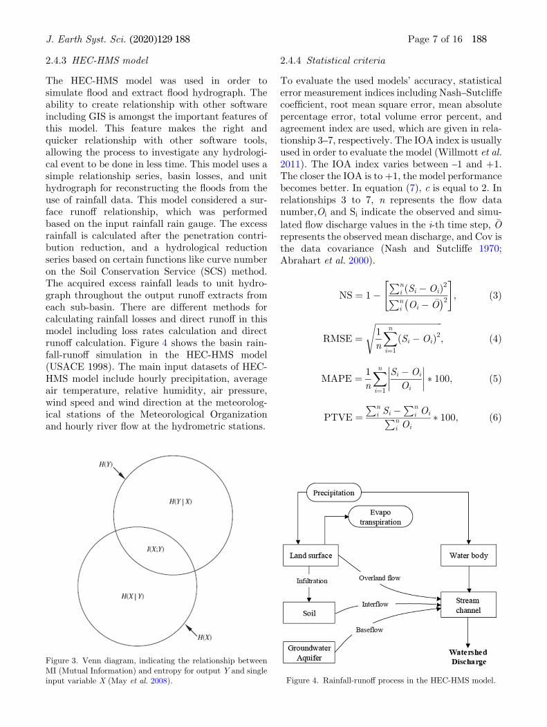
2.4.3 HEC-HMS model

The HEC-HMS model was used in order tosimulate Cood and extract Cood hydrograph. Theability to create relationship with other softwareincluding GIS is amongst the important features ofthis model. This feature makes the right andquicker relationship with other software tools,allowing the process to investigate any hydrologi-cal event to be done in less time. This model uses asimple relationship series, basin losses, and unithydrograph for reconstructing the Coods from theuse of rainfall data. This model considered a sur-face runoA relationship, which was performedbased on the input rainfall rain gauge. The excessrainfall is calculated after the penetration contri-bution reduction, and a hydrological reductionseries based on certain functions like curve numberon the Soil Conservation Service (SCS) method.The acquired excess rainfall leads to unit hydro-graph throughout the output runoA extracts fromeach sub-basin. There are different methods forcalculating rainfall losses and direct runoA in thismodel including loss rates calculation and directrunoA calculation. Figure 4 shows the basin rain-fall-runoA simulation in the HEC-HMS model(USACE 1998). The main input datasets of HEC-HMS model include hourly precipitation, averageair temperature, relative humidity, air pressure,wind speed and wind direction at the meteorolog-ical stations of the Meteorological Organizationand hourly river Cow at the hydrometric stations.

2.4.4 Statistical criteria

To evaluate the used models’ accuracy, statisticalerror measurement indices including Nash–SutcliAecoefBcient, root mean square error, mean absolutepercentage error, total volume error percent, andagreement index are used, which are given in rela-tionship 3–7, respectively. The IOA index is usuallyused in order to evaluate the model (Willmott et al.2011). The IOA index varies between –1 and +1.The closer the IOA is to +1, the model performancebecomes better. In equation (7), c is equal to 2. Inrelationships 3 to 7, n represents the Cow datanumber,Oi and Si indicate the observed and simu-

lated Cow discharge values in the i-th time step, �Orepresents the observed mean discharge, and Cov isthe data covariance (Nash and SutcliAe 1970;Abrahart et al. 2000).

NS ¼ 1�Pn

i Si �Oið Þ2Pni Oi � �O� �2

" #; ð3Þ

RMSE ¼ffiffiffiffiffiffiffiffiffiffiffiffiffiffiffiffiffiffiffiffiffiffiffiffiffiffiffiffiffiffiffiffi1

n

Xni¼1

Si �Oið Þ2s

; ð4Þ

MAPE ¼ 1

n

Xni¼1

Si �Oi

Oi

�� 100; ð5Þ

PTVE ¼Pn

i Si �Pn

i OiPni Oi

� 100; ð6Þ

Figure 3. Venn diagram, indicating the relationship betweenMI (Mutual Information) and entropy for output Y and singleinput variable X (May et al. 2008). Figure 4. Rainfall-runoA process in the HEC-HMS model.


IOA ¼1�

Pni¼1 Si �Oij j

cPn

i¼1 Oi � �O�� ;when

Xni¼1

Si �Oij j � cXni¼1

Oi � �O��

Pni¼1 Si �Oij jPni¼1 Oi � �O

�� 1;whenXni¼1

Si �Oij j[ cXni¼1

Oi � �O��

8>>>><>>>>:

ð7Þ

3. Results and discussion

3.1 Synoptic analysis: Rainfall and Coodon March 14 and 15, 2016

The synoptic structure at 00:00 on March 14presented a low pressure (state) of 1005 hPa withan elevation trough the 500 hPa levels in easternMediterranean (Bgure 5). On the same day at 12:00UTC, it extended to the east in the low-pressurestate, and one of its troughs extended to the centerof Iran and the second trough extended to the westof Iraq. Because of extending the elevation troughto Iran in the next 6 hr – 18:00 UTC – rainfall hadbegun in Karun-4 basin on March 14. It reinforcedin the low-pressure state and decreased to 995 hPaat 00:00 UTC on March 15. Its central core waslocated in the north of Iran and its elevation troughextended to the center of Iran. During this time,rainfall had increased in the basin. In the nextfew hours, it was transmitted to higher latitudesin the low-pressure state, and a pressure stackwas installed on Iran. Consequently, the highestamount of rainfall reported in Koohrang was at 46mm at 12:00 on March 15, after that the amount ofrainfall decreased and at 00:00 UTC on March 16,raining was over.

3.2 Calibration and validation of HEC-HMSmodel

First, before applying the HEC-HMS model forpredicting the Cood hydrograph, it was calibratedand veriBed. Calibration and veriBcation processcontinue to determine the optimal values of theparameters in HEC-HMS model. This processbegins with data collection. The required data forprecipitation-runoA models include rainfall data,current time series, air temperature time series,and so on. The next step in the calibration processis to select the initial values for the parameters. Bygiving the initial values of the model, it is able tocalculate the hydrograph of the basin runoA in allparts of the basin, especially the location of sta-tions with observational data. At this point, theobserved and the computational hydrograph were

compared. The main purpose of this comparisonwas to judge the good compliance with the actualhydrological system. If the compliance of thehydrographs was not satisfactory, the parametersshould be corrected and modiBed by an optimiza-tion method and the process repeated. Optimiza-tion operations can be performed manually andusing engineering judging by the frequent correc-tion of parameters or automatically by the model.When compliance is good and satisfactory, theoptimal and Bnal values of the parameters will bereported.In this model, some other models were used to

simulate the conversion of rainfall to runoA, pene-tration losses, baseline Cow and snow melting insub-basins known as the Clark unit hydrographmethod, soil conservation service (SCS) curvenumber method, subsidence method, and degree-day method, respectively. The Muskingum–Kungehydrologic model was also used for the Cow routingin rivers. Figure 6 indicates the sub-basins and theKarun-4 dam rivers upstream schematic con-structed in the HEC-HMS hydrologic model envi-ronment. Two heavy rainfall events of 9 Mar 2014and 8 Mar 2011 were considered for calibration andvalidation of HEC-HMS model, respectively. Thebasin monthly average rainfall of March 2011 andMarch 2014 was 88 and 82 mm, respectively.Figure 7 displays the comparison between the

observed and simulated Cood hydrograph on 9 Mar2014 event at the Armand hydrometric station formodel calibration. Rainfall-runoA simulation wascarried out for the validation time period with theBnal parameter’s values obtained from calibration,in order to validate the HEC-HMS calibratedmodel. Figure 7 presents the observed and simu-lated Cood hydrograph comparison on 8 Mar 2011event for model veriBcation at Armand hydro-metric station. In Bgure 7, it can be seen that Coodhydrograph variations, which were simulated byHEC-HMS model on 9 Mar 2014 event at theArmand hydrometric station were close to theobserved Cood hydrograph and HEC-HMS modelwas well calibrated in terms of rainfall-runoA sim-ulation. Also, due to the information of Bgure 8, itcan be found that Cood hydrograph variationssimulated by HEC-HMS model on 8 Mar 2011 isnear to observed Cood hydrograph.Table 4 displays the goodness-of-Bt statistical

criteria for calibration and veriBcation period ofHEC-HMS model in simulating Cow hydrograph atArmand hydrometric station. According to table 4,the Nash–SutcliAe coefBcient values, total volume


error percent, and mean absolute percentage errorbetween the observed and simulated hydrograph inthe calibration step were equal to 0.91, –4.27%, and8.85%, respectively. In addition, the negative valueof PTVE (percent of total volume error) indicateda low volume runoA estimate with the HEC-HMSmodel. Regarding Nash coefBcient and PTVE intable 4, which equals to 0.74, 0.19, respectively,can be demonstrated that HEC-HMS model waswell calibrated in the veriBcation step.

3.3 PMI algorithm results

In order to predict rainfall and air temperature atdifferent Karun-4 basin synoptic stations, hourlyrainfall, average air temperature, relative humid-ity, air pressure, wind speed, and wind direction foreach station were used. Each input variables

including rainfall hourly statistics, average airtemperature, relative humidity, air pressure, windspeed and wind direction at each station wereconsidered up to 24 hrs ago to provide the potentialset of input variables.The PMI algorithm was used in order to deter-

mine the input variables eAect on output variables(rainfall and air temperature amounts in the next6 hrs at each station). This algorithm determinesthe eAectiveness of input variables by calculatingthe PMI value. Table 5 displays the PMI algorithmresults for six eAective variables, by the order ofpriority in predicting rainfall at different stations.Table 6 shows the PMI algorithm results for sixeAective variables by the order of priority inpredicting air temperature at different stations.In tables 5 and 6, R(t) represents the current

rain status (current rainfall amounts), R(t�1)represents the rainfall amount of 6 hrs ago, R(t�2)

Figure 5. Free sea level pressure (Blled black line) hectopascal, geopotential height of 500 hPa levels (dashed line), winddirection 925 hPa (Picamen) for the times of 00:00 on March 14 (a), 12:00 on March 14 (b), 00:00 on March 15 (c), and 12:00 onMarch 15 (d).


represents the rainfall amount of 12 hrs ago,R(t�3) represents the rainfall amount of 18 hrsago, H(t) represents the current relative humidity,H(t�1) represents the relative humidity of 6 hrsago, T(t) represents the average amount of currentair temperature, T(t�1) represents the averageamount of air temperature 6 hrs ago, T(t�2) rep-resents the average amount of air temperature 12hrs ago, T(t�3) represents the average amount ofair temperature 18 hrs ago, WS(t) represents thecurrent wind speed, WS(t�1) represents the windspeed of 6 hrs ago, WS(t�2) represents the windspeed of 12 hrs ago, WD(t�4) represents the winddirection of 24 hrs ago, P(t�1) represents the airpressure of 6 hrs ago, and P(t�2) represents the airpressure of 12 hrs ago.According to table 5 and based on the

AIC(p) criterion, eAective input variables for

predicting rainfall at Shahrekord station areH(t) and R(t). The eAective input variables forpredicting rainfall at Borujen station are H(t),R(t) and R(t�1), respectively. The eAective inputvariables for predicting rainfall at Lordegan stationare R(t), R(t�1), and R(t�2), respectively. Also,the eAective input variables for predicting rainfallat Koohrang station are T(t�2), R(t), and R(t�1),respectively, for the temperature of 12 hrs ago.

Figure 6. Topology of sub-basins and rivers upstream of Karun-4 dam made in HEC-HMS model.

0

50

100

150

200

250

300

350

400

450

0 24 48 72 96 120 144 168 192 216 240 264 288

stre

amflo

w (c

ms)

�me (hr)

Observed

Simulated

Figure 7. Comparison between the observed and simulatedCood hydrograph in 9 Mar 2014 event at Armand station formodel calibration.

0

100

200

300

400

500

600

700

800

0 24 48 72 96 120 144 168 192 216 240 264

Stre

amflo

w (c

ms)

�me (hr)

Observed

Simulated

Figure 8. Comparison between the observed and simulatedCood hydrograph in 8 Mar 2011 event at Armand station formodel veriBcation.

Table 4. Goodness-of-Bt statistical criteria for calibration andvalidation period of HEC-HMS model.

Stage NS

PTVE

(%)

RMSE

(cms)

MAPE

(%)

Calibration 0.91 –4.27 21.5 8.85

Validation 0.74 0.19 63.5 25.70


Furthermore, as per the information of table 6,and also based on the AIC(p) criterion, theeAective input variables for predicting the airtemperature at Shahrekord and Boroujen stationsare T(t�3), T(t), and T(t�2), respectively. TheeAective input variables for predicting the airtemperature at Lordegan station are T(t�3), T(t),T(t�2), and T(t�1), respectively. Also, the eAec-tive input variables for predicting the air temper-ature at Koohrang station are T(t), T(t�3), andT(t�2), respectively.

3.4 ANN and SVM model structure

The model parameters in this study are the numberof hidden nodes (HN), themomentum (MM), and thelearning rate (a) for the ANN.Moreover, the positivetrade-oA parameter (C), the tolerance of the lossfunction (e), and the kernel function parameter (r)are used for the SVM. The trial-and-error methodwas employed for selecting the weighting factors andmodel parameters, which were allowed to vary asfollows: wTR, wCA[ [0.0, 1.0], HN [ [2, 20], a [ [0.0005,0.005], MM [ [0.0, 0.9], C [ [6.0, 14.0], e [ [0.07, 0.16],and r [ [2.0, 4.0]. The parameter set for each modelwas selected among 1000 combination sets of

parameters. The initial distribution of weights andbiases is also an important factor for the BPA-basedANN model building process when considering thelocal minimum problem. In this study, 100 randomsets were explored for each combination of modelparameters to select the best initial distribution ofweights and biases for ANN models. Table 7 sum-marizes the selected weighting factors and modelparameter sets for the Bve stations.

3.5 Comparison of model performances

The one-step ahead direct prediction results andthe recursive prediction results were systematicallycompared with the station observations. The modelperformance criteria using direct prediction withthe selected model parameters for the six stationswas estimated. Precipitation and temperaturedirect prediction results are shown in tables 8 and9. The Nash–SutcliAe model eDciency coefB-cient (NS) and Root Mean Square Error (RMSE)were used to assess the predictive power of hy-drological models. According to NS and RMSE,rainfall and temperature prediction by SVM isbetter than the ANN in some stations and for twoevents.

Table 5. Results of PMI algorithm to determine the eAective input variables for predicting rainfall atdifferent stations.

Shahrekord Boroojen Lordegan Koohrang

Variable AIC(p) Variable AIC(p) Variable AIC(p) Variable AIC(p)

H(t) –312.3 H(t) –738.6 R(t) –674.7 T(t–2) –1376.4

R(t) –492.9 R(t) –839.3 R(t–1) –733.3 R(t) –2153.5

R(t–1) –483.6 R(t–1) –840.3 R(t–2) –745.0 R(t–1) –2159.3

T(t) –1472.4 WS(t–2) –838.3 R(t–3) –721.9 R(t–2) –2099.9

T(t–1) –1386.8 WS(t–1) –978.2 H(t) –679.1 T(t) –2487.1

WS(t–1) –1205.1 WS(t) –1246.3 WS(t) –801.5 WD(t–4) –2442.8

Table 6. Results of PMI algorithm to determine the eAective input variables for predicting airtemperature at different stations.

Shahrekord Boroojen Lordegan Koohrang

Variable AIC(p) Variable AIC(p) Variable AIC(p) Variable AIC(p)

T(t–3) –7379.1 T(t–3) –7379.1 T(t–3) –3155.7 T(t) –8427.7

T(t) –8968.6 T(t) –8968.6 T(t) –3703.4 T(t–3) –11195.4

T(t–2) –9468.3 T(t–2) –9468.3 T(t–2) –4014.8 T(t–2) –11549.2

H(t) –9423.8 H(t) –9423.8 T(t–1) –4034.4 P(t–2) –11292.6

T(t–1) –9314.9 T(t–1) –9314.9 H(t–1) –3929.8 H(t) –10858.9

H(t–1) –9182.9 H(t–1) –9182.9 P(t–1) –3416.8 T(t–1) –10585.6


3.6 Results of WRF model

3.6.1 Comparison of the observed rainfalland temperature and model output

Table 10 shows the IOA index for the hourly pre-dicted rainfall with different schemas. The IOAcoefBcient of the observed rainfall and the modelwith eight schemas had a value of more than 0.5indicating their coordination at all stations exceptBoroujen. Out of eight schemes, the four MYJLD,MYJLG, MYJWD, and MYJWG schemes had thehighest values. The best IOA values were attainedat the amounts of 0.77, 0.76, 0.74, and 0.52 inShahrekord, Saman, Koohrang, and Lordegan,respectively, with the MYJLD schema. Boroujenhas a negative coefBcient and indicates a lack ofoutput coordination of the model with theobservation.Table 11 displays the r and IOA index for the

hourly predicted air temperature with differentschemas. The IOA index did not provide an

appropriate value for the hourly temperature esti-mation by the model. This means that the WRFmodel does not perform well on the temperatureprediction. Except the two stations of Saman andShahrekord, which had a coefBcient of 0.47 and0.52, respectively, all other stations, had the coef-Bcient of \0.5. The four MYJLG, MYJWG,YSULG, and YSUWG schemas provided a betterresult than the other four schemas.According to the information of table 12, the

observed peak discharge was 200 m3/s, andthe other two MYJLG and MYJWD schemas withthe values of about 6.220 and 3.233 m3/s werethe closest to the observation. The MYJLG schemaprovided a good result in the former cases, and theMYJWD schema had a good coordination with theobservational data in the case of rainfall. Conse-quently, the schemas predicted rainfall well duringthe whole period, and also had a good performanceon peak discharge. Moreover, the observed runoAheight was 3.45 mm and the two MYJLG and

Table 7. Selected input structure and model parameters.

Model ANN model parameters SVM model parameters

Station Variable HN LR MM W C e r

Shahrekord Rainfall 12 0.005 0.1 0.4 7 0.1 2.9

Temperature 10 0.002 0.5 0.3 5 0.04 2

Lordegan Rainfall 12 0.004 0.6 0.5 6.5 0.05 3.5

Temperature 10 0.001 0.2 0.4 7.5 0.09 4

Koohrang Rainfall 12 0.002 0.1 0.3 12 0.2 4

Temperature 10 0.004 0.2 0.4 14 0.1 3.5

Farsan Rainfall 12 0.001 0.1 0.3 10 0.09 4

Temperature 11 0.001 0.3 0.5 8 0.05 4

Boroojen Rainfall 12 0.004 0.4 0.4 9 0.07 3

Temperature 10 0.002 0.2 0.3 7 0.08 2

Ardal Rainfall 12 0.001 0.6 0.4 8 0.09 3.5

Temperature 10 0.002 0.4 0.3 7.5 0.1 4

Table 8. Direct prediction results for precipitation.

Event 15 Mar 2016

Model SVM ANN

Station RMSE NS RMSE NS

Shahrekord 0.62 1 1.2 0.9

Loordegan 1 0.9 0.48 1

Koohrang 2.62 1 2.65 1

Farsan 1.18 0.6 0.55 0.9

Broojen 0.16 0.8 0.41 –0.4

Ardal 1.79 0.7 0.8 0.9

Table 9. Direct prediction results for temperature.

Event 15 Mar 2016

Model SVM ANN

Station RMSE NS RMSE NS

Shahrekord 3.71 0 1.48 3.7

Loordegan 0.84 0.9 0.89 0.9

Koohrang 1.23 0.8 1.36 0.7

Farsan 1.36 0.7 0.8 1

Broojen 0.87 0.9 1.01 0.9

Ardal 1.65 0.7 0.92 0.9


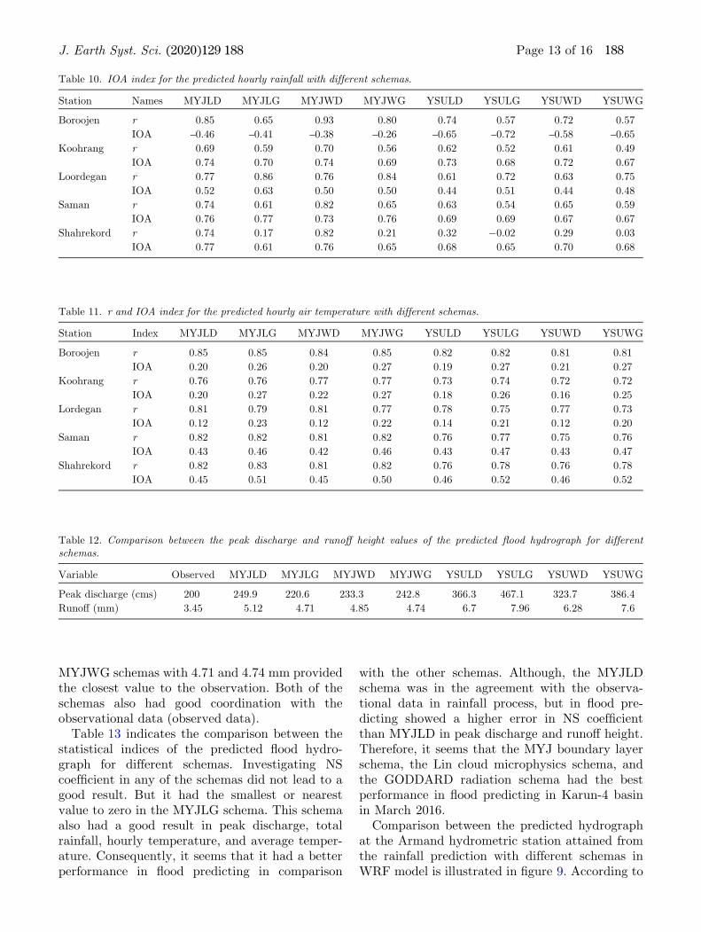
MYJWG schemas with 4.71 and 4.74 mm providedthe closest value to the observation. Both of theschemas also had good coordination with theobservational data (observed data).Table 13 indicates the comparison between the

statistical indices of the predicted Cood hydro-graph for different schemas. Investigating NScoefBcient in any of the schemas did not lead to agood result. But it had the smallest or nearestvalue to zero in the MYJLG schema. This schemaalso had a good result in peak discharge, totalrainfall, hourly temperature, and average temper-ature. Consequently, it seems that it had a betterperformance in Cood predicting in comparison

with the other schemas. Although, the MYJLDschema was in the agreement with the observa-tional data in rainfall process, but in Cood pre-dicting showed a higher error in NS coefBcientthan MYJLD in peak discharge and runoA height.Therefore, it seems that the MYJ boundary layerschema, the Lin cloud microphysics schema, andthe GODDARD radiation schema had the bestperformance in Cood predicting in Karun-4 basinin March 2016.Comparison between the predicted hydrograph

at the Armand hydrometric station attained fromthe rainfall prediction with different schemas inWRF model is illustrated in Bgure 9. According to

Table 10. IOA index for the predicted hourly rainfall with different schemas.

Station Names MYJLD MYJLG MYJWD MYJWG YSULD YSULG YSUWD YSUWG

Boroojen r 0.85 0.65 0.93 0.80 0.74 0.57 0.72 0.57

IOA –0.46 –0.41 –0.38 –0.26 –0.65 –0.72 –0.58 –0.65

Koohrang r 0.69 0.59 0.70 0.56 0.62 0.52 0.61 0.49

IOA 0.74 0.70 0.74 0.69 0.73 0.68 0.72 0.67

Loordegan r 0.77 0.86 0.76 0.84 0.61 0.72 0.63 0.75

IOA 0.52 0.63 0.50 0.50 0.44 0.51 0.44 0.48

Saman r 0.74 0.61 0.82 0.65 0.63 0.54 0.65 0.59

IOA 0.76 0.77 0.73 0.76 0.69 0.69 0.67 0.67

Shahrekord r 0.74 0.17 0.82 0.21 0.32 �0.02 0.29 0.03

IOA 0.77 0.61 0.76 0.65 0.68 0.65 0.70 0.68

Table 11. r and IOA index for the predicted hourly air temperature with different schemas.

Station Index MYJLD MYJLG MYJWD MYJWG YSULD YSULG YSUWD YSUWG

Boroojen r 0.85 0.85 0.84 0.85 0.82 0.82 0.81 0.81

IOA 0.20 0.26 0.20 0.27 0.19 0.27 0.21 0.27

Koohrang r 0.76 0.76 0.77 0.77 0.73 0.74 0.72 0.72

IOA 0.20 0.27 0.22 0.27 0.18 0.26 0.16 0.25

Lordegan r 0.81 0.79 0.81 0.77 0.78 0.75 0.77 0.73

IOA 0.12 0.23 0.12 0.22 0.14 0.21 0.12 0.20

Saman r 0.82 0.82 0.81 0.82 0.76 0.77 0.75 0.76

IOA 0.43 0.46 0.42 0.46 0.43 0.47 0.43 0.47

Shahrekord r 0.82 0.83 0.81 0.82 0.76 0.78 0.76 0.78

IOA 0.45 0.51 0.45 0.50 0.46 0.52 0.46 0.52

Table 12. Comparison between the peak discharge and runoA height values of the predicted Cood hydrograph for differentschemas.

Variable Observed MYJLD MYJLG MYJWD MYJWG YSULD YSULG YSUWD YSUWG

Peak discharge (cms) 200 249.9 220.6 233.3 242.8 366.3 467.1 323.7 386.4

RunoA (mm) 3.45 5.12 4.71 4.85 4.74 6.7 7.96 6.28 7.6


the all schemas prediction, the amount of runoAwas more than the observed one (observationaldata). Also, runoA start time in the model wasearlier than the observed one (observational data).The runoA variations process obtained from eachof the eight schemes was similar, but their runoAheight was different. The most inappropriateschema was the YSULG.

3.7 Comparison between the predicted Coodhydrograph with SVM and ANN and WRFmodels

Figure 10 displays the predicted Cood hydrographat the Armand hydrometric station with inputweather variables from including WRF, SVM andANN models. SVM model hydrograph variationswere nearer to the observed hydrograph than theother models.Table 14 displays the comparison between the

peak discharge and runoA height values of thepredicted Cood hydrograph in different models.According to the data shown in table 15, SVMmodel had more accuracy in runoA height pre-dicting than the other two models of WRF andANN. Table 15 also shows the comparison betweenthe statistical indices of the predicted Coodhydrograph in different models. The Nash–SutcliAe

coefBcient value for WRF, SVM, and ANN modelswas –0.293, 0.548, and –0.607, respectively. TheRMSE value between the observed and predictedCow discharge values by WRF, SVM, and ANNmodels was as 37, 21.9, and 41.3 m3/s, respectively.Also, percent of total volume error (PTVE)between the observed and predicted Cow dischargevalues by the use of WRF, SVM, and ANN modelswas 30.95, 15.59, and 32.14%, respectively.Therefore, the SVM model had more accuracy inrainfall and air temperature predicting, and alsoCood hydrograph in comparison with the othermodels.

Table 13. Comparison between the predicted Cood hydrograph statistical indices for different schemas.

Criteria MYJLD MYJLG MYJWD MYJWG YSULD YSULG YSUWD YSUWG

NS –1.208 –0.293 –0.519 –0.483 –8.893 18.471 –6.082 –14.657

RMSE std dev 1.5 1.1 1.2 1.2 3.1 4.4 2.7 4

PTVE (%) 42.73 30.95 34.96 31.81 88.29 124.7 76.15 114.29

RMSE (cms) 48.4 37.0 40.1 39.7 102.4 143.7 86.7 128.9

MAPE (%) 42.91 31.93 35.92 32.79 82.70 116.60 73.00 109.62

0

50

100

150

200

250

300

350

400

450

500

0 20 40 60 80 100

Fore

cast

ed st

ream

flow

(cm

s)

Time (hr)

ObservedMYJLDMYJLGMYJWDMYJWGYSULDYSULGYSUWDYSUWG

Figure 9. Comparison between the predicted hydrograph at Armand hydrometric station obtained from rainfall prediction withdifferent schemas in WRF model.

0

50

100

150

200

250

300

0 24 48 72 96

fore

cast

ed st

ream

flow

(cm

s)

�me (hr)

observed

WRF model (MYJLG)

SVM

ANN

Figure 10. Comparison between the predicted hydrograph atthe Armand hydrometric station in different models.


4. Discussion and conclusion

The purpose of this paper was to evaluate andcompare different models based on data drivenmodel including ANN and SVM and WRFnumerical model in short-term prediction of pre-cipitation values and air temperature in groundstations in order to evaluate more accurate modeland using output of these model to forecast of Coodhydrograph. According to the results of this study,the accuracy of the SVM model in predicting pre-cipitation and air temperature and Cood hydro-graphy is higher than the WRF model. In addition,the time required to run the SVM model in theshort-term forecast of precipitation and air tem-perature is much lower than the WRF model. Theresults obtained from the rainfall and air temper-ature prediction and also the prediction of Cood byusing different schemas of WRF model, indicatedthat MYJLG scheme was more accurate than theother schemas. Therefore, it seems that the MYJboundary layer scheme, the Lin cloud micro phy-sics scheme, and the GODDARD radiationscheme had the best performance in Cood predict-ing in Karun-4 basin on March 2016. The results ofusing PMI algorithm for determining the eDcientinput variables in order to predict rainfall at raingauge stations in the next 6 hrs, revealed theeAective variables as relative humidity, the currentrainfall (the current rain status), the rainfall of

6 hrs ago, and the rainfall and temperature of12 hrs ago. Also, the PMI algorithm results for airtemperature predicting in the next 6 hrs indicatedthat the eAective input variables included thetemperature of 18 hrs ago, the current tempera-ture, the temperature of 12 hrs ago, and the tem-perature of 6 hrs ago. The results indicated thatusing the PMI algorithm for determining theeAective input variables in ANN and SVM models,caused a significant reduction in the time needed todetermine the eAective variables, and consequentlyallowed the model development. Comparisonbetween the peak discharge and runoA height val-ues of the predicted Cood hydrograph in differentmodels revealed that the SVM model had moreeDciency and accuracy in rainfall, air temperature,and Cood hydrograph predicting than other mod-els. In addition, the WRF model accuracy in rain-fall, air temperature, and Cood hydrographpredicting was more than ANN model. Due to thefact that the WRF model requires a relatively longtime to run to predict rainfall and air temperature,using the simple SVM model reduces the timerequired for short-term forecasting of rainfall andair temperature values and the results could beused for Cood forecast.

References

Abrahart R J and See L 2000 Comparing neural network andautoregressive moving average techniques for the provisionof continuous river Cow forecasts in two contrastingcatchments; Hydrol. Process. 14 2157–2172.

Afandi G E, Mostafa M and Hussieny F E 2013 Heavy rainfallsimulation over Sinai peninsula using the weather researchand forecasting model; Int. J. Atmos. Sci. 2013 1–11.

Chang T K, Talei A, Alaghmand S and Ooi M P L 2017 Choiceof rainfall inputs for event-based rainfall-runoA modelingin a catchment with multiple rainfall stations using data-driven techniques; J. Hydrol. 545 100–108.

Cover T M and Thomas J A 1991 Information theory andstatistics. Elements of Information Theory (1st edn) Cover TM and Thomas J A (eds); JohnWiley and Sons, pp. 279–335.

Das S, Ashrit R, Iyengar G R, Mohandas S, Gupta M D,George J P, Rajagopal E and Dutta S K 2008 Skills ofdifferent mesoscale models over Indian region duringmonsoon season: Forecast errors; J. Earth Syst. Sci. 117603–620.

Du J, Liu Y, Yu Y and Yan W 2017 A prediction ofprecipitation data based on support vector machine andparticle swarm optimization (PSO-SVM) algorithms;Algorithms 10 57.

Givati A, Lyan B, Liu Y and Rimmer A 2012 Using the WRFmodel in an operational streamCow forecast system for theJordan River; J. Appl. Meteorol. Climatol. 51 285–299.

Table 14. Comparison between peak discharge and runoAheight values of the predicted Cood hydrograph in differentmodels.

Variable Observed

WRF

(MYJLG) SVM ANN

Peak discharge

(cms)

200 220.6 244.2 285.2

RunoA height

(mm)

3.45 4.71 4.05 4.62

Table 15. Comparison between the statistical indices of thepredicted Cood hydrograph in different models.

Statistical criteria WRF (MYJLG) SVM ANN

NS –0.293 0.548 –0.607

RMSE std dev 1.1 0.7 1.3

PTVE (%) 30.95 15.59 32.14

RMSE (cms) 37.0 21.9 41.3

MAPE (%) 31.93 14.33 29.26


Hong S Y and Lee J W 2009 Assessment of the WRF model inreproducing a Cash-Cood heavy rainfall event over Korea;Atmos. Res. 93 818–831.

Kisi O and Cimen M 2012 Precipitation forecasting by usingwavelet-support vector machine conjunction model; Eng.Appl. Artif. Intell. 25 783–792.

Li L, Gochis D J, Sobolowski S and Mesquita M D 2017Evaluating the present annual water budget of a Himalayanheadwater river basin using a high-resolution atmosphere-hydrology model; J. Geophys. Res. 122 4786–4807.

Lu K and Wang L 2011 A Novel Nonlinear CombinationModel Based on Support Vector Machine for RainfallPrediction, 2011 Fourth International Joint Conference onComputational Sciences and Optimization, Yunnan,pp. 1343–1346, https://doi.org/10.1109/CSO.2011.50.

Lu T, Yamada T and Yamada T 2016 Fundamental study ofreal-time short-term rainfall prediction system in water-shed: Case study of Kinu watershed in Japan; ProcediaEngineering 154 88–93.

May R J, Dandy G C, Maier H R and Nixon J B 2008Application of partial mutual information variable selectionto ANN forecasting of water quality in water distributionsystems; Environ. Model. Softw. 23(10–11) 1289–1299.

Moser B A, Gallus W A J and Mantilla R 2015 An initialassessment of radar data assimilation on warm seasonrainfall forecasts for use in hydrologic models; Wea.Forecasting 30 1491–1520.

Mourre L, Condom T, Junquas C, Lebel T, Sicart J E,Figueroa R and Cochachin A 2015 Spatio-temporal assess-ment of WRF, TRMM and in-situ precipitation data in atropical mountain environment (Cordillera Blanca, Peru);Hydrol. Earth Syst. Sci. 12 6635–6681.

Nash J E and SutcliAe J V 1970 River Cow forecasting throughconceptual model. Part 1 – A discussion of principles;J. Hydrol. 10 282–290.

Nayak D R, Mahapatra A and Mishra P 2013 A Survey onrainfall prediction using artiBcial neural network; Int.J. Comput. Appl. 72 32–40.

Papadopoulos A, Serpetzoglou E and Anagnostou E N 2009Evaluating the impact of lightning data assimilation onmesoscale model simulations of a Cash Cood inducing storm;Atmos. Res. 94 715–725.

Ratna S B, Ratnam J V, Behera S K, Rautenbach C J,Ndarana T, Takahashi K and Yamagata T 2014 Perfor-mance assessment of three convective parameterizationschemes in WRF for downscaling summer rainfall overSouth Africa; Clim. Dyn. 42 2931–2953.

Sassanian S, Azadi M, Asgarishirazi H and Mirzai A 2015Evaluation of the performance of the WRF model with ninedifferent physical conBgurations to predict winter precipi-tation in southwestern Iran; J. Sci. Technol. 90 1–11.

Seo J H, Lee J H and Kim J H 2014 Feature selection for veryshort-term heavy rainfall prediction using evolutionarycomputation; Adv. Meteorol. 2014 1–15.

Shannon C E 1948 A mathematical theory of communication;Bell Syst. Tech. J. 27 379–423.

Sharma A, Luk K C, Cordery I and Lall U 2000 Seasonal tointerannual rainfall probabilistic forecasts for improvedwater supply management: Part 2 – Predictor identiBcationof quarterly rainfall using ocean-atmosphere information;J. Hydrol. 239 240–248.

Sivapragasam C, Liong S and Pasha M 2001 Rainfall andrunoA forecasting with SSA-SVM approach; J. Hydroinf.141–152.

Taghavi F, Neyestani A and Ghader S 2013 Short rangeprecipitation forecasts evaluation of WRF model over Iran;J. Earth Space Phy. 39(2) 145–170.

Tan Q F, Lei X H, Wang X, Wang H, Wen X, Ji Y and KangA Q 2018 An adaptive middle and long-term runoA forecastmodel using EEMD-ANN hybrid approach; J. Hydrol. 567767–780.

Tian J, Jia L, Denghua Y, Liuqian D and Chuanzhe L 2019Ensemble Cood forecasting based on a coupled atmospheric-hydrological modeling system with data assimilation;Atmos. Res. 224 127–137.

Venkatesan C, Raskar S D and Tambe S S 1997 Prediction ofall India summer monsoon rainfall using error-back-propa-gation neural networks;Meteorol. Atmos. Phys. 62 225–240.

Willmott C J, Robeson S M and Matsuura K 2011 A reBnedindex of model performance; Int. J. Climatol. 32 2088–2094.

Wu C L and Chau K W 2013 Prediction of rainfall time seriesusing modular soft computing methods; Eng. Appl. ArtiB-cial Intelligence 26 997–1007.

Wu J, Lu G and Wu Z 2014 Flood forecasts based on multi-model ensemble precipitation forecasting using a coupledatmospheric-hydrological modeling system; Nat. Hazards74 325–340.

Yesubabu V, Srinivas C V, Langodan S and Hoteit I 2016Predicting extreme rainfall events over Jeddah, SaudiArabia: Impact of data assimilation with conventionaland satellite observations; Quart. J. Roy. Meteorol. Soc.142 327–348.

Young C C, Liu W C and Wu M C 2017 A physically basedand machine learning hybrid approach for accurate rainfall-runoA modeling during extreme typhoon events; Appl. SoftComput. 53 205–216.

Yucel I, Onen A, Yilmaz K K and Gochis D J 2015 Calibrationand evaluation of a Cood forecasting system: Utility ofnumerical weather prediction model, data assimilation andsatellite-based rainfall; J. Hydrol. 523 49–66.

Zakeri Z, Freedom M and Sahraeian F 2014 VeriBcation of theWRF output for rainfall in Iran during February-end ofMay 2009; J. Sci. Technol. 9 86–87.

Zhou J, Zhang H, Zhang J, Zeng X, Ye L, Liu Y, Tayyab Mand Chen Y 2018 WRF model for precipitation simulationand its application in real-time Cood forecasting in theJinshajiang River Basin, China; Meteorol. Atmos. Phys.130 635–674.

Corresponding editor: N V CHALAPATHI RAO


https://doi.org/10.1109/CSO.2011.50

evaluation of wrf and artificial intelligence models in

Documents