evla radio frequency interference survey from 1-8 ghz...
TRANSCRIPT

National Radio Astronomy Observatory Student Cooperative Education Program
EVLA Radio Frequency Interference Survey From 1 -8 GHz, Analysis of EMS System Noise
Figure and VLA L-Band Feed Horns
V UA X. <r\ ~1 * r < f t/vx ( eC. rv\"o
Eric Reynolds University of New Mexico Undergraduate
Albuquerque, NM December 28,2001
National Radio Astronomy Observatory (NRAO) VLA/VLBA Electronics Division
Interference Protection Group (Front End)
University of New Mexico Department of Electrical and Computer Engineering


EVLA Radio Frequency Interference Survey From 1 -8 GHz, Analysis of EMS System Noise
Figure and VLA L-Band Feed Horns
Eric ReynoldsCo-op Period: August 1,2001 through December 28, 2001
Mr. Daniel Mertely, EE NRAO Project Supervisor


Acknowledgements
I would like to thank everyone that helped me during my co-op period. I would
like to thank everyone that let me borrow tools and parts. I greatly appreciate the
assistance I received from the antenna mechanics. I would also like to thank Clifford
Serna, for providing interesting conversation and spotting wildlife on the many trips I
made to the VLA. Thanks to Bill Brundage for helping me determine the EMS system
noise temperature, and for checking my work with the EVLA RFI survey. Special thanks
to Kerry Shores and Nathan Thomas for showing me the ropes of IPG and NRAO.
Thanks to Dan Mertely for his supervision and guidance. And thanks to Raul
Armendariz, Dan Mertely, Clint Janes, and the National Science Foundation for giving
me this co-op opportunity.


Summary
This document covers the work done during my co-op employment at NRAO.
Two major projects were accomplished: an RF interference survey from 1 - 8 GHz for
the Expanded VLA, and digitizing the radiation patterns of the VLA L-band feed horns.
Included in this document are examples of RF Engineering theory that I learned
throughout my co-op experience. Perhaps this document this document will be of use for
future co-op employees of NRAO.


Table of Contents
Part 1: Radio Frequency Interference Survey 1 - 8 GHz at the VLA......................1-36Abstract, Introduction................................................................................................1Section I: The Environmental Monitoring Station (EMS)........................................2-5
1.1 Introduction...................................................................................................... 21.2 Current EMS Components................................................................................3-4
1.2.1 Antennas.................................................................................................. 31.2.2 Cable “EMS-2”.........................................................................................31.2.3 Front End................................................................................................. 31.2.4 Cable “EMS-X”....................................................................................... 3-41.2.5 Receiver................................................................................................... 4
1.3 Predicted System Noise Figure.........................................................................4-51.3.1 System Setup for Noise Floor Prediction.................................................41.3.2 Theoretical Noise Floor Calculation........................................................4-5
1.4 Data Acquisition.............................................................................................. 5Section II: Power Flux Density Plots 1 - 8 GHz.......................................................6-31
2.1 Introduction....................................................................................................... 62.2 DME (1-1 .2 GHz).......................................................................................... 6-7
2.2.1 DME Frequency Allocations....................................................................62.2.2 RFI Summary, DME............................................................................... 62.2.3 DME PFD Plots...................................................................................... 7
2.3 L-Band.............................................................................................................8-142.3.1 RFI Summary, L-Band........................................................................... 82.3.2 Frequency Allocations, 1.2 - 1.4 GHz....................................................92.3.3 Frequency Allocations, 1.4 - 1.6 GHz....................................................92.3.4 PFD Plots, 1.2- 1.6GHz...................................................................... 10-112.3.5 RFI Summary, 1.2 - 1.6 GHz.................................................................112.3.6 Frequency Allocations, 1.6 - 1.8 GHz...................................................122.3.7 RFI Summary, 1.6 - 1.8 GHz................................................................122.3.8 PFD Plots, 1 .6- 1.8 GHz...................................................................... 132.3.9 Frequency Allocations, 1.8 - 2 GHz.....................................................142.3.10 PFD Plots, 1 .8 -2 GHz.........................................................................14
2.4 S-Band...........................................................................................................15-222.4.1 RFI Summary, S-Band.......................................................................... 122.4.2 Frequency Allocations, 2 - 2.4 GHz......................................................162.4.3 PFD Plots, 2 - 2.4 GHz..........................................................................172.4.4 Frequency Allocations, 2.4 - 2.6 GHz.................................................. 182.4.5 PFD Plots, 2.4 - 2.6 GHz......................................................................182.4.6 Frequency Allocations, 2.6 - 3 GHz.....................................................192.4.7 RFI Summary, 2.6 - 3 GHz................................................................. 192.4.8 PFD Plots, 1.6 - 3 GHz....................................................................... 202.4.9 Frequency Allocations, 3 - 4 GHz...................................................... 21
v


2.4.10 RFI Summary, 3 - 4 GHz.................................................................... 212.4.11 PFD Plots, 3 - 4 GHz...........................................................................22
2.5 C-Band.......................................................................................................... 23-302.5.1 Frequency Allocations, 4 - 5 GHz.......................................................232.5.2 RFI Summary, 4 - 5 GHz..................................................................... 232.5.3 PFD Plots, 4 - 5 GHz...........................................................................242.5.4 Frequency Allocations, 5 - 6 GHz.......................................................252.5.5 RFI Summary, 5 - 6 GHz.................................................................... 252.5.6 PFD Plots, 5 - 6 GHz...........................................................................262.5.7 Frequency Allocations, 6 - 7 GHz....................................................... 272.5.8 RFI Summary, 6 - 7 GHz.................................................................... 272.5.9 PFD Plots, 6 - 7 GHz.......................................................................... 282.5.10 Frequency Allocations, 7 - 8 GHz...................................................... 292.5.11 PFD Plots, 7 - 8 GHz..........................................................................30
2.6 RFI Summary, 1 - 8 GHz............................................................................31Section III Analysis of the EMS System Noise Temperature............................. 32-34
3.1 Introduction.................................................................................................323.2 Actual Noise Figure Calculation................................................................. 32-333.3 Comparison of Theoretical and Actual Noise Figures................................ 34
Section IV: Recommendations for Monitoring Above 8 GHz............................35-364.1 Introduction.................................................................................................354.2 RFI Monitoring 8 -1 2 GHz........................................................................354.3 RFI Monitoring 12-18 GHz......................................................................35-364.4 RFI Monitoring 18-40 GHz......................................................................36
Part 2: Analysis of the Pattern Characteristics in the L-Band Feed Horns.........37-42Introduction..........................................................................................................37Section I: Method for Directivity and Beam Efficiency Calculations................38-39Section II: Summary of Directivity and Beam Efficiency Approximations.......39-42
APPENDIX A: EMS Path and Antenna Characterizations...................................43-46APPENDIX B: List of References and Sources.................................................... 48


List of Figures
Figure 1: EMS System Block Diagram.......................................................................2Figure 2: DME Peak Hold Plots...................................................................................7Figure 3: 24 Hour Peak Hold L-Band Plot...................................................................8Figure 4: Peak Hold Plots, 1.2 - 1.5 GHz...................................................................10Figure 5: Peak Hold Plots, 1.4 - 1.6 GHz...................................................................11Figure 6: Peak Hold Plots, 1.5 - 1.8 GHz...................................................................13Figure 7: Peak Hold Plots, 1 .8 -2 GHz..................................................................... 14Figure 8: 24 Hour Peak Hold S-Band Plot...................................................................15Figure 9: Peak Hold Plots, 2 - 2.4 GHz..................................................................... 17Figure 10: Peak Hold Plots, 2.4 - 2.6 GHz................................................................. 18Figure 11: Peak Hold Plots, 2.6 - 3 GHz..................................................................... 20Figure 12: 24 Hour Peak Hold Plots, 3 - 4 GHz...........................................................22Figure 13: 24 Hour Peak Hold Plots, 4 - 5 GHz...........................................................24Figure 14: 24 Hour Peak Hold Plots, 5 - 6 GHz...........................................................26Figure 15: 24 Hour Peak Hold Plots, 6 - 7 GHz...........................................................28Figure 16: 24 Hour Peak Hold Plots, 7 - 8 GHz...........................................................30Figure 17: Example Radiation Pattern of a VLA L-Band Feed Horn...........................37
List o f TablesTable 1: EMS Setup for 2 - 3 GHz Monitoring...........................................................4Table 2: Frequency Allocations, 960 - 1215 MHz.......................................................6Table 3: Frequency Allocations, 960 - 1400 MHz.......................................................9Table 4: Frequency Allocations, 1 4 0 0 -1530 MHz................................................... 9Table 5: Frequency Allocations, 1610-1715 MHz................................................... 12Table 6: Frequency Allocations, 1710-2110 MHz................................................... 14Table 7: Frequency Allocations, 2110 - 2400 MHz................................................... 16Table 8: Frequency Allocations, 2400 - 2655 MHz................................................... 18Table 9: Frequency Allocations, 2655 - 3100 MHz................................................... 19Table 10: Frequency Allocations, 3.1 -4 .2 GHz........................................................ 21Table 11: Frequency Allocations, 4.2 - 5 GHz............................................................. 23Table 12: Frequency Allocations, 5 - 5.925 GHz........................................................ 25Table 13: Frequency Allocations, 5.925 - 7.075 GHz................................................. 27Table 14: Frequency Allocations, 7.9 - 8.025 GHz.................................................... 29Table 15: RFI Summary, 1 - 8 GHz............................................................................ 31Table 16: Comparison of Theoretical and Actual Noise Figures................................ 34Table 18: Summary of Directivity Calculations, 1.35 GHz..........................................40Table 19: Summary of Directivity Calculations, 1.53 GHz..........................................41Table 20: Summary of Directivity Calculations, 1.72 GHz..........................................42


Part 1
Radio Frequency Interference Survey 1-8 GHz at the VLA
Abstract
The IPG group at the AOC has been assigned to determine characteristics of
external RF interference that the expanded VLA should expect. The plan was to survey
RFI from 1-50 GHz, covering each of the eight EVLA receiver bands. As of August,
2001, the survey has begun. Data is now available from 1-8 GHz, and preparations are
being made to survey frequencies above 8 GHz. New sources of RFI have been observed
and located. Plots of RFI power flux density (PFD) versus frequency are available for
public viewing on the NRAO web page at:
http://www.aoc.nrao.edu/via/interference/survey
The data sets for each of the PFD plots are also available from the above URL.
Many of the RFI plots are also in this document along with frequency allocation
information, and a description of some of the strongest interference signals.
Introduction
Radio Astronomy has always been very vulnerable to RF interference. Radar,
wireless communication, mobile satellite service, and other radio technology continue to
develop, causing more interference to radio astronomy and the EVLA. With the
characteristics of interference known, one can compensate in EVLA development and
design. Hopefully the data in the survey will also be useful to astronomers in observing.
This document consists of four sections:
Section I describes the current Environmental Monitoring Station (EMS) used in the
survey. The method of acquiring and processing the data is also discussed.
1

Section II contains power flux density (PFD) plots of RF interference from 1-8 GHz.
Frequency allocation information and an RFI analysis accompany each plot. Section III
contains an analysis of the EMS system noise figure. Section IV contains
recommendations for acquiring RF interference data for frequencies above 8 GHz.
Section I: The Environmental Monitoring Station (EMS)
1.1 Introduction
The EMS was created by students in the NRAO co-op program. Each semester
new improvements have been added. After many ups and downs, the system is now
operating from 1-12 GHz. Some of the downs include periodic receiver failure, non
existent characterization data for antennas, and the collapse of the tower. Replacements,
repairs, and adjustments have been made to get the system operational. Figure (1) is a
block diagram of the system. The system is located at the southeast side of the VLA,
near the dormitories. The antennas are located on a 50-foot Rohn Tower. The receiver
and PC’s are located in the RFI shelter, a metal building located near the tower.
Antenna
heliaxCable
FrontEnd
HefiaxCable
SpectrumAnalyzer
Figure 1: EMS System Block Diagram
2

1.2 Current EMS Components
In order of signal path, here is a brief description of each component in the EMS. See
Appendix A for the EMS characterization data. Detailed characterization information on
the components of EMS is available in the IPG office.
1.2.1 Antennas
For 1-8 GHz data, the antenna used was a Dome & Margolinl-8 GHz RCP omni
directional, conical log spiral. The antenna has right hand circular polarization. Its
azimuth and elevation patterns have been professionally characterized at 2.1 GHz, 4
GHz, and 8 GHz. Raul Armendariz & Nathan Thomas from the IPG GROUP
characterized its gain versus frequency. See Appendix A for a table of gain and effective
aperture versus frequency. The effective aperture was used in calculating power flux
density. An antenna was not available for measurements above 8 GHz. Two standard
gain horns (8.2-12.4 and 12.4-18 GHz) have been ordered for survey use from 8-18 GHz.
A dual ridged waveguide horn is available for monitoring from 18-40 GHz.
1.2.2 Cable “EMS-2” LDF2-50Q
“EMS-2” is an 11 ft., 7 in. long 3/8” heliax cable that runs from the output of the
1-8 GHz omni antenna to the input of the front end.
1.2.3 Front End
The front end was designed by Kerry Shores and built by Raul Armendariz. It
operates from 5 MHz to 13 GHz. It is remotely switchable from seven different bands
starting with P-band and ending with X-band. Complete characterization data for the
front end is available in the IPG office.
1.2.4 Cable “EMS-X”
3

“EMS-X” is a 62 ft. long 3/8” heliax cable that runs from the output of the front
end to the input of the spectrum analyzer.
1.2.5 Receiver
The receiver is an HP 70001 spectrum analyzer. The internal preamplifier was
used and the spectrum analyzer was in peak hold mode. As a whole, the receiver noise
temperature at 2.5 GHz is approximately 2300 K.
1.3 Predicted System Noise Figure
Here is the calculation to predict the EMS system noise figure at 2500 MHz. This
prediction is done assuming system settings identical to the system settings used to obtain
one of the plots in Section II (see Figure 8, pg 15). This is the system setup:
1.3.1 System Setup for Noise Floor Prediction
EMS path S-Band
Frequency Range 2 - 3 GHz
Resolution Bandwidth 215 kHz
Video Bandwidth 300 kHz
Spectrum Analyzer Attenuation OdB
Spectrum Analyzer Preamplifier On
Spectrum Analyzer Mode Peak Hold
Table 1: EMS setup for 2-3 GHz monitoring
1.3.2 Theoretical Noise Fioor Calculation
The following equation was used to predict the system temperature (refer to Figure 1):
T sys = T a + T c i + T lna + T c2_____ + ______ T sa________G ci (G ci)(G lna) (G ci)(G ln a)(G c2)
Where:
4

T a = 150 K (approximate noise temperature of the antenna)
G lna = 38 dB = 6309 (gain of the S-Band amplifier at 2.5 GHz)
Gci = -2 dB = 0.631 (loss of cable “EMS-2” at 2.5 GHz)
Gc2 = -5 dB = 0.316 (loss of cable “EMS-X” at 2.5 GHz)
T lna = 260 K (noise temp, of the S-Band low noise amplifier in the EMS front end)
Tci = (290/Gci) - 290 = 169.59 K (noise temperature of cable “EMS-2” at 2.5 GHz)
T c 2 = (290/GC2) - 290 = 627.72 K (noise temperature of cable “EMS-X” at 2.5 GHz)
T sa = 2290 K (approximate noise temperature of the spectrum analyzer at 2.5 GHz)
Plugging in the parameters to the equation yields:
T sys = 150K + 169.59K + 260K + 627.72K + 2290K_______0.631 (0.631)(6309) (0.631 )(6309)(0.316)
T sys = 734 K
This is a prediction of what the system noise temperature will be at 2500 MHz. In
Section III a comparison will be made between the above predicted noise temperature
and the approximate actual noise temperature.
1.4 Data Acquisition
A serial connection from the spectrum analyzer to a PC transfers the data in
ASCH text format. A program was written to display two columns: frequency bin (0-
1023) and power (dBm). Knowing the frequency settings (span and center frequency)
from the spectrum analyzer, each frequency bin can be associated with a frequency. The
data is then calibrated, accounting for the net loss and gain and the antenna effective
aperture, resulting with power flux density (W/mA2). The following equation was used:
PFD * Ae = Prx The calibration was done manually in Microsoft Excel.
Appendix A contains the system losses and gains, and the antenna effective aperture.
5

Section II: Power Flux Density (PFD) Plots 1-8 GHz
2.1 PFD Plots.. Allocation Information, RFI Analysis
This section contains RF interference plots obtained through the EMS system.
Frequency allocation information is also provided. The plots are organized according to
their associated band. There are plots for L-Band, S-Band, and C-Band. Low L-Band
plots (1-1.2 GHz) have been given their own section because of the significant interest in
DME radar interference. All of the following plots are taken with the spectrum analyzer
in peak hold mode. The interference may look worse than it actually is because of
intermittent signals detected in peak hold mode. A signal that occurs briefly will be
recorded in peak hold mode. Above each plot is information on when and for how long
the data was taken.
2.2 DME (1-1.2 GHz)
2.2.1 DME Frequency Allocations
Allocation Information RFI Description, Characteristic960 -1215 MHz1
• Aeronautical RadionavigationIntermittent
Table 2: Frequency Allocations, 960 -1215 MHz2.2.2 RFI Summary, DME
DME (Distance Measuring Equipment) provides pilots with range in nautical
miles. It also contributes a large amount of interference to the VLA. The interrogator
signals are intermittent. The two transponder signals are at 1030 and 1090 MHz. The
IPG group is working on a way to retrieve data at high resolution to study transient
characteristics of DME and other interfering signals.
1 AH frequency allocations in bold letters indicate bands where RFI was detected. Allocations obtained from Spectrum Guide, by Bennett Z. Kobb. 3rd Edition, New Signals Press, 1996
6

2.2.3 DME PFD Plots
DME (1-1.2 GHz)
Data taken week of 8/12/01 by Eric Reynolds (AOC).Power Flux Density (PFD) calculated to produce measured dBm power into Spectrum Analyzer.
EM S Path: L-Band Low Gain & M'rteq 18dB amplifier at SA input.Spectrum Analyzer set in Peak-Hold mode for 20 minutes.
SPAN: 200MHz RBW: 10kHz
Frequency (MHz)
DME (1-1.2 GHz)Data taken week of 8/19/01 by Eric Reynolds (AOC).
Power Flux Density (PFD) calculated to produce measured dBm power into Spectrum Analyzer. EMS Path: L-Band Low Gain
Spectrum Analyzer set in Peak-Hold mode for 20 minutes.
SPAN: 200MHz RBW: 10kHz
Frequency (MHz)
Figure 2: DME Peak Hold Plots
7

2.3 L-Band ( 1 - 2 GHz)
1-2GHZData taken week of 10/01/01 by Eric Reynolds (AOC).
Power Flux Density (PFD) calculated to produce measured dBm power into Spectrum Analyzer. EM S Path: L-Band Low Gain
Spectrum Analyzer set in Peak-Hold mode for 24 hours.
SPAN: 1000MHz RBW: 215kHz
Frequency (MHz)
Figure 3: 24 Hour Peak Hold L-Band Plot
2.3.1 RFI Summary. L-Band
The most significant RFI in L-band is from the low frequencies (1000 - 1200
MHz). The low L-band signals are Distance Measuring Equipment (DME). Other
sources of RFI in L-band are the Global Positioning System (GPS) from 1215 - 1240
MHz, aeronautical radionavigation from 1300 - 1350 MHz, and the Iridium satellite
communications system from 1621.35 - 1626.5 MHz. Many studies have already been
made with L-band RFI and can be found in the IPG office.
8

2.3.2 Frequency Allocations, 1.2 -1 .4 GHz
Allocation Information RFI Description, Characteristic960-1215 MHz
• Aeronautical RadionavigationIntermittent
1215-1240 MHz• Radionavigation Satellite• Global Positioning System (GPS)
Intermittent
1240-1300 MHz• Radiolocation• Amateur Radio
1300-1350 MHz• Aeronautical Radionavigation• Radiolocation
Intermittent
1350-1400 MHz• Radiolocation• Fixed and Mobile services• FAA and Air Force JSS radar network
Table 3: Frequency Allocations, 960 -1400 MHz
2.3.3 Frequency Allocations. 1.4 -1 .6 GHz
Allocation Information RFI Description, Characteristic1400-1427 MHz
• Radio Astronomy1427 - 1429 MHz
• Space Operation• Fixed and Mobile services• Private Land Mobile• Satellite Communications
1429- 1435 MHz• Fixed and Mobile services• Private Land Mobile
1435 - 1525 MHZ• Mobile services
1525-1530 MHz• Mobile services• Satellite Communications
Table 4: Frequency Allocations, 1400 - 1530 MHz
9

2.3.4 PFD Plots. 1.2 - 1.6 GHz
PFD(dBWAnA2)
PFD(dBWAnA2)
1.2-1.4 GHzData taken week of 10A31A31 by Eric Reynolds (AOC).
Power Flux Density (PFD) calculated to produce measured dBm power into Spectrum Analyzer. EMS Path: L-Band Low Gain
Spectrum Analyzer set in Peak-Hold mode for 20 minutes.
Frequency (MHz)
1.3-1.5 GHzData taken week of 10A31A31 by Eric Reynolds (AOC).
Power Flux Density (PFD) calculated to produce measured dBm power into Spectrum Analyzer. EMS Path: L-Band High Gain
Spectrum Analyzer set in Peak-Hold mode for 20 minutes.
SPAN. 200MHz RBW. 100kHz
Frequency (MHz)
Figure 4: Peak Hold Plots, 1.2 - 1.5 GHz
10

1.4-1.6 GHzData taken week of 10/01£)1 by Eric Reynolds (AOC).
Power Flux Density (PFD) calculated to produce measured dBm power from Spectrum Analyzer. EM S Path: L-Band Low Gain
Spectrum Analyzer set in Peak-Hold mode for 20 minutes.
SPAN: 200 MHz RBW: 100kHz
Frequency (MHz)
Figure 5: Peak Hold Plots, 1.4 - 1.6 GHz
2.3.5 RFI Summary. 1.2 - 1.6 GHz:
Most of the RFI from 1.2 - 1.4 GHz is caused by aeronautical radionavigation.
The signals are intermittent and relatively strong. No RFI was detected from 1.4 - 1.6
GHz.
11

2.3.6 Frequency Allocations, 1.6 - 1.8 GHz
Allocation Information RFI Description, Characteristic1610-1626.5 MHz
• Satellite Communication.Big LEO Spectrum (Iridium, Glonass)
• Aeronautical Radionavigation
Continual
1626.5 -1645.5 MHz• Maritime Mobile Satellite• Satellite Communication
1645.5 -1646.5 MHz • Mobile Satellite
1646.5 -1660 MHz• Aeronautical Mobile Satellite
1660-1660.5 MHz• Aeronautical Mobile Satellite• Radio Astronomy
1660.5 -1668.4 MHz• Radio Astronomy• Space Research
1668.4 - 1670 MHz• Radio Astronomy• Meteorological Aids (radiosonde)
1670 - 1700 MHz• Meteorological Aids (radiosonde)• Meteorological Satellite
1700-1710 MHz• Fixed Services• Meteorological Satellite
Table 5: Frequency Allocations, 1610 -1715 MHz
2.3.7 RFI Summary, 1.6 - 1.8 GHz:
The only RFI found in 1.6 - 1.8 GHz is from 1621.65 - 1626.5 GHz from the
Iridium satellite communications system.
12

2.3.8 PFD Plots. 1.6 - 1.8 GHz
1.5-1.7 GHzData taken week of 1CMD1/01 by Eric Reynolds (AOC).
Power Flux Density (PFD) calculated to produce measured dBm power into Spectrum Analyzer. EM S Path: L-Band High Gain
Spectrum Analyzer set in Peak-Hold mode for 20 minutes.
Frequency (MHz)
1.6-1.8 GHzData taken week of 10AD1 A)1 by Eric Reynolds (AOC)
Power Flux Density (PFD) calculated to produce measured dBm power into Spectrum Analyzer. EMS Path: L-Band Low Gain
Spectrum Analyzer set in Peak-Hold mode for 20 minutes
Frequency (MHz)
Figure 6: Peak Hold Plots, 1.5 - 1.8 GHz
13

2.3.9 Frequency Allocations, 1.8 - 2 GHz
Allocation Information RFI Description,Characteristic1710-1850 MHz
• Fixed and Mobile servicesContinual
1850-1990 MHz• Fixed and Mobile services• Personal Communications Services• Private Operational Fixed Services• RF Devices
1990-2110 MHz• Fixed and Mobile services• Auxiliary Broadcast (74) Cable Television (78)
Table 6: Frequency Allocations, 1710 - 2110 MHz
2.3.10 PFD Plots, 1.8 - 2 GHz
1.8-2 GHzData taken week of 10AJ1/01 by Eric Reynolds (AOC).
Power Flux Density (PFD) calculated to produce measured dBm power into Spectrum Analyzer. EMS Path: L-Band Low Gain
Spectrum Analyzer set in Peak-Hold mode for 20 minutes.
Frequency (MHz)
Figure 7: Peak Hold Plot, 1.8 - 2 GHz
14

2.4 S-Band ( 2 - 4 GHz)
PFD(dBMMnA2)
PFD(dBWftnA2)
2-3GHZData taken week of 10/01AD1 by Eric Reynolds (AOC).
Power Flux Oensity (PFD) calculated to produce measured dBm power into Spectrum Analyzer. EM S Path: S-Band
Spectrum Analyzer set in Peak-Hold mode for 24 hours.
SPAN: 1000MHz RBW: 215kHz
Frequency (MHz)
3-4GHzData taken week of 11A3&01 by Enc Reynolds (AOC).
Power Flux Density (PFD) calculated to produce measured dBm power into Spectrum Analyzer. EMS Path: S-Band
Spectrum Analyzer set in Peak-Hold mode for 24 hours.
SPAN: 1000MHz RBW. 215kHz
Frequency (MHz)
Figure 8: 24 Hour Peak Hold S-Band Plots
15

2.4.1 RFI Summary. S-Band
The major RFI in S-Band is from radars. NEXRAD Doppler Radar operates at
2740 and 2790 MHz, resulting in strong, intermittent RFI at the VLA. Defense radar
signals were found from 3.1 - 3.6 GHz. They were strong, but seldom present.
2.4.2 Frequency Allocations. 2 -2 .4 GHzAllocation Information RFI Description,Characteristic2110-2150 MHz
• Fixed and Mobile services• Private Operational Fixed Services• Domestic Public Fixed Services• Public Mobile Services
2150-2160 MHz• Fixed Services• Private Operational Fixed Services• Multipoint Distribution
2160 - 2200 MHz• Fixed and Mobile services• Domestic Public Fixed Services• Private Operational Fixed Services• Public Mobile Services
2200-2290 MHz• Fixed and Mobile services• Space Research and Operation• Earth Exploration Satellite
2290-2300 MHz• Fixed and Mobile services• Space Research
2300-2310 MHz• Amateur Radio
2310 - 2360 MHz• Fixed and Mobile services• Radiolocation• Broadcasting-Satellite• Digital Audio Radio Services
Continual
2360-2390 MHz• Fixed and Mobile services• Radiolocation
2390 - 2400 MHz• Amateur Radio
Table 7: Frequency Allocations, 2110 - 2400 MHz
16

2.4.3 PFD Plots. 2 - 2.4 GHz242 GHz
Data taken week of 1CMD1/01 by Eric Reynolds (AOC).Power Flux Density (PFD) calculated to produce measured dBm power into Spectrum Analyzer.
EMS Path: S-Band Spectrum Analyzer set in Peak-Hold mode for 20 minutes.
22-2.4 GHzData taken week of 10/01A31 by Eric Reynolds (AOC).
Power Flux Density (PFD) calculated to produce measured dBm power into Spectrum Analyzer. EMS Path: S-Band
Spectrum Analyzer set in Peak-Hold mode for 20 minutes.
PFD (dBW/mA2)
-40
-50
-60
-70
-80
-90
-100
-110
-120
-130
-140
SPAN: 200MHz RBW: 100kHz
Frequency (MHz)
Figure 9: Peak Hold Plots, 2 - 2.4 GHz
17

2.4.4 Frequency Allocations, 2.4 - 2.6 GHz
Allocation Information RFI Description,Characteristic2400 - 2402 MHz
• Amateur Radio2402-2417 MHz
• Amateur Radio• Radiolocation
2450-2483.5 MHz• Fixed and Mobile services• Radiolocation
2483.5-2500 MHz• Radiodetermination Satellite• Mobile Satellite• Satellite Communication
2500-2655 MHz• Fixed services• Broadcasting-Satellite• Auxiliary Broadcasting• Domestic Public Fixed Services
Table 8: Frequency Allocations, 2400 - 2655 MHz 2.4.5 PFD Plots. 2.4 - 2.6 GHz
2.4-2.6GHZ Data taken week of 11/05AJ1 by Eric Reynolds (AOC).
Power Flux Density (PFD) calculated to produce measured dBm power into Spectrum Analyzer. EMS Path. S-Band
Spectrum Analyzer set in Peak-Hold mode for 20 minutes.
SPAN: 200MHz RBW: 100kHz
Frequency (MHz)
Figure 10: Peak Hold Plot 2.4 - 2.6 GHz
18

2.4.6 Frequency Allocations, 2.6 - 3 GHzAllocation Information RFI Description,Characteristic2655-2690 MHz
• Earth Exploration Satellite• Radio Astronomy• Space Research• Fixed services• Broadcasting-Satellite• Auxiliary Broadcasting• Private Operational Fixed Services
2690 - 2700 MHz• Earth Exploration Satellite• Radio Astronomy• Space Research
2700-2900 MHz• Aeronautical Radionavigation• Meteorological Aids• Radiolocation
Intermittent
2900-3100 MHz• Maritime Radionavigation• Radiolocation
Table 9: Frequency Allocations, 2655 - 3100 MHz
2.4.7 RFI Summary. 2.6 - 3 GHz
The RFI in this band is from the next generation Doppler radar (NEXRAD) at 2740 and
2790 MHz. The signals are intermittent and relatively strong.
19

2.4.8 PFD Plots, 2,6 - 3 GHz
2.6-2.8GHZData taken week of 11/05A)1 by Eric Reynolds (AOC).
Power Flux Density (PFD) calculated to produce measured dBm power into Spectrum Analyzer. EMS Path: S-Band
Spectrum Analyzer set in Peak-Hold mode for 20 minutes.
SPAN: 200MHz RBW: 100kHz
Frequency (MHz)
2.8-3GHZData taken week of 11^35 5̂1 by Eric Reynolds (AOC).
Power Flux Density (PFD) calculated to produce measured dBm power into Spectrum Analyzer. EMS Path: S-Band
Spectrum Analyzer set in Peak-Hold mode for 20 minutes.
SPAN: 200MHz RBW: 100kHz
Frequency (MHz)
Figure 11: Peak Hold Plots, 2.6 - 3 GHz
20

2.4.9 Frequency Allocations, 3 - 4 GHz
Allocation Information RFI Description,Characteristic3.1-3 .3 GHz
• RadiolocationSeldom Present
3.3-3.5 GHz• Radiolocation• Amateur Radio
Seldom Present
3.5-3 .6 GHz• Aeronautical Radionavigation• Radiolocation
3 .6 -3 .7 GHz• Aeronautical Radionavigation• Radiolocation• Fixed Satellite
3 .7 -4 .2 GHz• Fixed Services• Fixed Satellite• Domestic Public Fixed Services• Satellite Communications• Private Operational Fixed Services
Table 10: Frequency Allocations, 3.1 - 4.2 GHz
2.4.10 RFI Summary, 3 - 4 GHz
The RFI (3.1 - 3.3 GHz) in this band is from defense radar. The signals are detected only when the monitoring system is set in peak hold mode for 24 hours.
21

2.4.11 PFD Plots. 3 - 4 GHz
3-4GHZData taken week of 10/01A31 by Eric Reynolds (AOC).
Power Flux Density (PFD) calculated to produce measured dBm power into Spectrum Analyzer. EM S Path: S-Band
Spectrum Analyzer set in Peak-Hold mode for 24 hours.
34GHzData taken week of 11/DS/01 by Eric Reynolds (AOC).
Power Flux Density (PFD) calculated to produce measured dBm power into Spectrum Analyzer. EMS Path: S-Band
Spectrum Analyzer set in Peak-Hold mode for 24 hours.
SPAN 1000MHz RBW 215kHz
Frequency (MHz)
Figure 12: 24 Hour Peak Hold Plots, 3 -4 GHz
22

2.5 C-Band (4- 8 GHz)
2.5.1 Frequency Allocations. 4 - 5 GHz
Allocation Information RFI Description,Characteristic4 .2 -4 .4 GHz
• Aeronautical Radionavigation• Aviation
Continual
4 .4 -4 .5 GHz• Fixed and Mobile Services
4 .5-4 .66 GHz• Fixed and Mobile Services• Fixed-Satellite
4 .66-4 .8 GHz• Fixed and Mobile Services• Fixed-Satellite
4 .8-4 .99 GHz• Fixed and Mobile Services
Intermittent
4 .9 9 -5 GHz• Radio Astronomy• Space Research
Table 11: Frequency Allocations, 4.2 - 5 GHz
2.5.2 RFI Summary. 4 - 5 GHz:
Interference in the 4.2 - 4.4 GHz band is caused by aeronautical radionavigation. The
4.8 - 4.99 GHz band sees interference from communication services from the
Departments of Defense, Energy, and the Treasury.
23
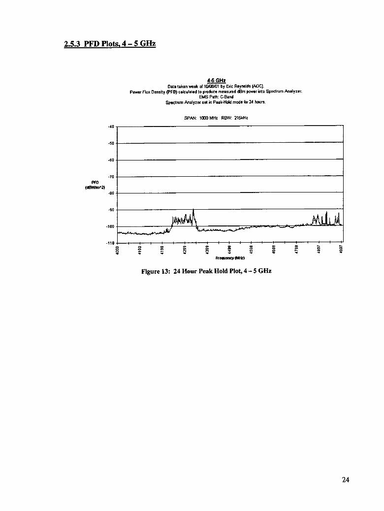
2.5.3 PFD Plots. 4 - 5 GHz
PFD(dflWAnA2)
Data taken week of 10A38/D1 by Eric Reynolds (AOC).Power Flux Density (PFD) calculated to produce measured dBm power into Spectrum Analyzer.
EMS Path: 0-Band Spectrum Analyzer set in Peak-Hold mode for 24 hours.
4-6 GHz
SPAN: 1000 MHz RBW: 215kHz
Figure 13: 24 Hour Peak Hold Plot, 4 - 5 GHz
24

2.5.4 Frequency Allocations, 5 - 6 GHz
Allocation Information RFI Description,Characteristic5 - 5.25 GHz
• Aeronautical Radionavigation• Aviation
Seldom Present
5.25-5.35 GHZ• Radiolocation
5.35 - 5.46 GHz• Aeronautical Radionavigation• Aviation• Radiolocation
Seldom Present
5.46-5.47 GHz• Radionavigation• Radiolocation
Seldom Present
5.47-5.6 GHz• Maritime Radionavigation• Radiolocation
Seldom Present
5.6-5.65 GHz• Maritime Radionavigation• Radiolocation• Meteorological Aids
Seldom Present
5.65-5.85 GHz• Radiolocation• Amateur Radio
Seldom Present
5.85 - 5.925 GHz• Radiolocation• Amateur Radio• Fixed-Satellite
Table 12: Frequency Allocations, 5 - 5.925 GHz
2.5.5 RFI Summary. 5 - 6 GHz
The RFI from 5 - 6 GHz is only detected when the system is in peak hold mode
for 24 hours.
25

2.5.6 PFD Plots. 5 - 6 GHz
Data taken week of 10A38/01 by Eric Reynolds (AOC).Power Flux Density (PFD) calculated to produce measured dBm power into Spectrum Analyzer.
EMS Path: C-Band Spectrum Analyzer set in Peak-Hold mode for 24 hours.
5-6 GHz
SPAN: 1000MHz RBW: 215kHz
Frequency (MHz)
Figure 14: 24 Hour Peak Hold Plot, 5 - 6 GHz
26

2.5.7 Frequency Allocations, 6 - 7 GHz
Allocation Information RFI Description,Characteristic5.925-6.425 GHz
• Fixed Services• Fixed-Satellite• Domestic Public Fixed Services• Satellite Communications• Private Operational Fixed Services
6.425 - 6.525 GHz• Fixed-Satellite• Mobile Services• Domestic Public Fixed Services• Auxiliary Broadcast Cable Television• Private Operational Fixed Services
Seldom Present
6.525-6.875 GHz• Fixed Services• Fixed-Satellite• Domestic Public Fixed Services• Satellite Communications• Private Operational Fixed Services
6.875-7.075 GHz• Fixed and Mobile Services• Fixed-Satellite• Domestic Public Fixed Services• Auxiliary Broadcast Cable Television
Table 13: Frequency Allocations, 5.925 - 7.075 GHz
2.5.8 RFI Summary. 6 - 7 GHz
The RFI from 6 - 7 GHz is only detected when the system is in peak hold mode
for 24 hours. The source is unknown.
27

2.5.9 PFD Plots. 6 - 7 GHz
PFD(d8WAnA2)
6-7 GHzData taken week of KMD8/01 by Eric Reynolds (AOC).
Power Flux Density (PFD) calculated to produce measured dBm power into Spectrum Analyzer. EMS Path: C-Band
Spectrum Analyzer set in Peak-Hold mode for 24 hours.
Frequency (MHz)
Figure 15: 24 Hour Peak Hold Plot, 6 - 7 GHz
28

2.5.10 Frequency Allocations, 7 - 8 GHz
Allocation Information RFI Description,Characteristic7.075-7.125 GHz
• Fixed and Mobile Services• Domestic Public Fixed Services• Auxiliary Broadcast Cable Television
7.125-7.19 GHz• Fixed Services
7.19-7.235 GHz• Fixed Services• Space Research
7.235-7.25 GHz• Fixed Services
7.25-7.3 GHz• Fixed-Satellite• Mobile-Satellite
7 .3-7.45 GHz• Fixed Services• Fixed-Satellite• Mobile-Satellite
7.45-7.55 GHz• Fixed Services• Fixed-Satellite• Meteorological-Satellite• Mobile-Satellite
7.55-7.75 GHz• Fixed Services• Fixed-Satellite• Mobile-Satellite
7.75-7.9 GHz• Fixed Services
7.9 - 8.025 GHz• Fixed Services• Fixed-Satellite• Mobile-Satellite
Table 14: Frequency Allocations, 7.9 - 8.025 GHz
29
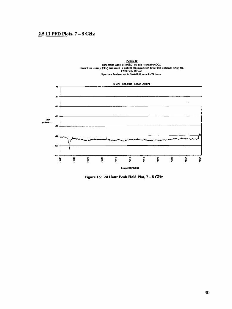
2.5.11 PFD Plots. 7 - 8 GHz
PFO(d8UttnA2)
Data taken week of 10A36/D1 by Eric Reynolds (AOC).Power Flux Density (PFD) calculated to produce measured dBm power into Spectrum Analyzer.
EMS Path: C-Band Spectrum Analyzer set in Peak-Hold mode for 24 hours.
7-8 GHz
SPAN. 1000MHz RBW: 215kHz
Frequency (MHz)
Figure 16: 24 Hour Peak Hold Plot, 7 - 8 GHz
30

The following table summarizes the RFI found in the survey. For each band that
had RH, the frequency and power flux density of the strongest peaks are recorded in the
table below.
2.6 RFI Summary, 1 - 8 GHz
Band(MHz)
Frequency(MHz)
PFD(dBW/mA2)
SignalCharacteristic
Source
960-1215 1030.1 -107 intermittent DME960-1215 1103.4 -96 intermittent DME960-1215 1090.5 -103 intermittent DME960-1215 1202.5 -103 intermittent GPS1215-1240 1233.2 -92 intermittent GPS1240-13001300-1350 1309.5 -93 intermittent aeronautical radionavigation1300-1350 1329.5 -91 intermittent aeronautical radionavigation1350-1610
1610-1626.5 1626 -99 continual Iridium1626-17101710-1850 1838.5 -104 continual Unknown1850 - 23102310-2360 2328.6 -100 continual unknown2360 - 2700
2700 - 2900 2740..6 -82 intermittentN EXRAD Doppler Radar,
aeronautical radionavigation
2700 - 2900 2789.1 -94 intermittentNEXRAD Doppler Radar,
aeronautical radionavigation2900-31003100 -3500 3218.9 -57 intermittent radiolocation, amateur3700 - 42004200 - 4400 4337.2 -90 continual aeronautical radionavigation4400 - 48004800 - 4990 4932.6 -92 intermittent Fixed & Mobile Services4990 - 52505250 - 5850 5338 -90 intermittent airborne weather radar5250 - 5850 5622.7 -74 intermittent airborne weather radar5850 - 64256425 - 6875 6439.9 -44 seldom present unknown6425 - 6875 6699.9 -48 seldom present unknown6875 - 79007900 - 8025 7991.2 -88 seldom present FAA
Table 15: RFI Summary, 1 - 8 GHz
31

Section III: Analysis of the EMS System Noise Temperature
3.1 Introduction
This section contains an approximate calculation of the EMS system noise
temperature at selected frequencies based on some of the PFD plots from Section II.
These values will be compared to the predicted noise temperature calculations from
Section I. The method of approximating the noise temperature will be shown using the
same frequency and system settings from the calculation of Section I (pg. 4). The system
settings produced the plot in Figure 8.
3.2 Actual Noise Figure Calculation
The following equations were used for frequency 2500 MHz:
(1) Pnoise = PFD * Ae
(2) Pnoise = k*Tpk*B, Tpk = Pnoise(k*B)
where:
Tpk = noise temperature with the spectrum analyzer in peak hold.
PFD = -106 dBW/mA2 = 2.5E-11 W/mA2 (approximate average value from plot, Fig. 8)
Ae = 1.4E-3 mA2 (Measured value for l-8GHz omni conical spiral. Used in calibrating
PFD data at 2.5GHz)
k= 1.38E-23 W*s/K (Boltzmann’s constant)
B = 215 kHz (Resolution bandwidth used)
32

Plugging in to equation (1), Pnoise = PFD * Ae:
Pnoise = (2.5E-11 W/mA2)*(1.4E-3 mA2)
Pnoise = 3.57E-14W
Plugging into equation (2), Tpk = Pnoise(k*B)
Tpk= ________(3.57E-14 W)_______[(1.38E-23 W*s/K)*(215000Hz)]
Tpk = 12,032 K
This is for peak hold data. In order to estimate the average system noise temperature, an
approximate ratio of peak/average data for the same spectrum analyzer settings was
obtained at 2500 MHz:
peak/a vg. = 12dB =16
Now an approximation for the average system noise temperature can be made:
T sys = Tpk/16
T sys = 12.032 K 16
T sys= 752 K
This is an approximation of the system noise temperature at 2500 MHz based on
the measurements in Figure 8. This value is fairly close to the predicted value of
734 K obtained in Section I. Table 16 is a comparison of predicted and actual
noise temperature approximations at selected frequencies in other EMS bands.
33

3.3 Comparison of Theoretical and Actual Noise Figures
EMS Band Plot
(Figure #)
Frequency Theoretical
Noise Figure
Actual
Noise Figure
L-Band Low Gain
( 1 - 2 GHz)
Fig. 3 1500 MHz 9.7 dB = 2400 K 11.9 dB = 4183 K
L-Band High Gain
(1.265 -1.835 GHz)
Fig. 5 1500 MHz 4.9 dB = 609 K 3.2 dB = 318 K
S-Band
( 2 - 4 GHz)
Fig. 8 2500 MHz 5.5 dB = 734 K 5.6 dB = 752 K
C-Band
(4 -1 0 GHz)
Fig. 15 6000 MHz 6.9 dB = 1141 K 8.6 dB = 1830 K
Table 16: Comparison of Theoretical and Actual Noise Figures
The second column in the above table refers to the plot used to calculate the noise
figure. The noise temperature in the L-Band Low Gain path is very high. This is because
the amplifier in this path has a very small gain (= 8 dB) and a fairly high noise
temperature (= 750 K). The gain of the LNA is not high enough to contribute in lowering
the noise floor of the spectrum analyzer. The actual noise floor was higher than the
predicted noise floor for a number of reasons. Some noise was unaccounted for and
could not be predicted. Also, the existence of RF interference will raise the noise floor of
the system.
34

4.1 Introduction
Due to the current setup of the Environmental Monitoring System, RF
interference data could not be taken for frequencies higher than 8 GHz. This section
contains suggestions for surveying these higher frequencies.
4.2 RFI Monitoring 8 - 1 2 GHz:
An RFI survey from 8 - 1 2 GHz can be accomplished in the near future. The
only two items needed are a low noise amplifier (LNA) and an antenna.
A Miteq 35 dB amplifier is available in the IPG lab that operates from 6 - 1 8
GHz. It has a noise figure close to 1.2 dB (92 K). A path has been included in the
current EMS front end for an amplifier to operate from 10 - 12 GHz. This amplifier
simply needs to be installed in the current front end.
Two standard gain horn antennas have been purchased and are expected to arrive
some time in January 2002. One of the antennas operate from 8 - 12.4 GHz and will be
used for RFI monitoring.
4.3 RFI Monitoring 12 - 18 GHz:
The Miteq 6 - 1 8 GHz amplifier described above can be used in the front end.
The other standard gain horn that was purchased operates from 12.4 - 18 GHz, and will
arrive in January. Two significant changes will need to be done for monitoring above 12
GHz. The two parts of EMS that will need to be replaced are the RF coaxial switches in
the front end and the heliax cables.
The RF switches in the front end operate up to 12.4 GHz. These will need to be
replaced with switches that can operate at higher frequencies.
Section IV: Recommendations for Monitoring Above 8 GHz
35

There are two heliax cables in EMS. EMS-2 is the 3/8” cable from the antenna to
the front end and EMS-X is the 3/8” cable from the front end to the spectrum analyzer.
These cables operate up to 13 GHz. The cables can be replaced with Vi” heliax, which
generally operates up to 20 GHz.
4.4 RFI Monitoring 18 - 40 GHz
The spectrum analyzer operates up to 22 GHz. Spectrum analyzers are very
expensive, so it is impractical to purchase a new spectrum analyzer that operates up to 40
GHz. Perhaps IPG can borrow one or find one in government surplus. A better solution
is down converting. This will require a mixer and a local oscillator (LO) between the
antenna and the front end. The signals would need to be down converted to a maximum
of 20 GHz in order to use the EMS front end, V6” heliax cables, and spectrum analyzer.
This means that an LO of 20 GHz would be required. Kerry Shores and Nathan Thomas
are currently working on the design of a renovated EMS system.
An antenna is available that operates from 18-40 GHz. The antenna is an
EMCO double-ridged waveguide horn that was purchased by IPG in June 2001.
36

Part 2
Analysis of the Pattern Characteristics in the L-Band Feed Horns
Introduction
A small project I did as a co-op was digitize the antenna radiation patterns of
three of the L-Band feed horns currently used in the VLA. Sri Srikanth, the designer of
the new L-Band feed horns for the EVLA, requested this. The radiation patterns of the
VLA L-band feed horns were measured in the 1970’s. These patterns are just analog
plots. Sri wanted discrete data points to put in the software he uses. I took samples of 1°
for H-plane and E-plane cuts at three frequencies for three different feed horns. This
helped in the design of the EVLA L-band feed horns. Here is an example of what one of
the patterns looks like:
Part No. 727000 Serial No. 4 H-Plane Cut 1.35 GHz
azimuth angle (theta)
Figure 17: Example Radiation Pattern of a VLA L-Band Feed Horn
37

Section I: Method for Directivity and Beam Efficiency Calculations
With the normalized power radiation patterns digitized, there is now a way to
approximate the directivity and beam efficiency of the VLA L-band feed horns. The
directivity is the value of the directive gain in the direction of its maximum value.
The following equation was used to calculate the directivity2:
D = ______ 4n______ = ______ 4n______ (1)Q a jf Pn (8, <j>)sin0d0d<j>
where: Qa = H Pn (0, (j>)sin0d0d<)) = beam area
Pn (0, <|>) = normalized power radiation pattern
d0 = change in 0 from 0 to n
d<j> = change in <j> from 0 to 2n
The patterns that were digitized were 2-dimensional cuts in E-plane and H-plane.
Assuming that the patterns are symmetrical and there is no variation in <j>, the integral
with respect to <J> is 2n. Equation (1) reduces to:
D = ______ 4k______2n I Pn (0)sin0d0
where 0 is from 0 to n (0° to 180°)
Pn (0) has been digitized, and the integral of a discrete function is the sum of each
discrete value. Discrete samples were taken every 1° from 0° to 90°. For points between
90° and 180°, an average value of -40dB, -50dB, or -60dB was assumed. The
approximate directivity can then be given by:
_________ 4k___________
2 Antennas, by John D. Kraus 2nd Edition, McGraw-Hill 1988, pg.101 - 102
38

D = m=18027t(7t/l 80) X Pn (0m)sin0m
m=0
This is an approximation using discrete samples from half (0° to 180°) of a radiation
pattern similar to the one in Figure 17. This approximation was done on the other half of
the radiation pattern as well, and similar values were obtained. The same method was
used for H-plane and E-plane cuts, and similar values were obtained. Due to the dynamic
range of the pattern measurement, data that had a value less than -40 dB could not be
recorded. For this data, an approximate average value of -4 0 , -50, or -60 dB was
assumed.
Beam efficiency can also be approximated. Beam efficiency is the ratio of the
main beam area to the total beam area. The following equation was used:
8 m = Q m
Qa
Where:
m=180
Ha = 27c(7c/l 80) £ Pn (0m)sin0m = The total beam area from 0° to 180°.m=0
m=9
Qm = 27t(7i;/9) X Pn (0m)sin0m = The main beam area from 0° to 9°.m=0
Section II; Summary of Directivity and Beam Efficiency Approximations
On the next page is a summary of the directivity and beam efficiency calculations
for one of the L-band feed horns. The directivity and beam efficiency are approximated
from radiation patterns from three L-band frequencies; 1.35, 1.53, and 1.72 GHz. For
each frequency, there is an H-Plane cut and an E-Plane cut. For both E-Plane and H-
39

Plane cuts, an approximation of directivity is made using the right and left hand half of
the pattern.
Part No. 727000 Serial No. 4
-40 dB: Condition where the approximate average value assumed for gains less than -40 dB was -4(-50 dB: Condition where the approximate average value assumed for gains less than -40 dB was -5C-60 dB: Condition where the approximate average value assumed for gains less than -40 dB was -6C+: Condition where the total beam area was approximated using 1 degree samples from 0 to 1£
degrees on the right hand half of the pattern.- : Condition where the total beam area was approximated using 1 degree samples from 0 to U
degrees on the left hand half of the pattern.avg: The average of right and left hand values
Table 17: Explanations of the Assumed Conditions for Directivity Calculations
Directivity and Beam Efficiency Approximations
1.35 GHZ __ ___Table 18
ConditionDirectivityApproximation
Directivity Approximation (dB)
BeamEfficiency Approximation
E-Plane Cut455.14 26.58145005 0.766-40 dB +
-40 dB - 434.69 26.38179649 0.739-40 dB avg 444.915 26.48277048 0.7525-50 dB + 464.74 26.67210054 0.783-50 dB - 443.75 26.47138366 0.755-50 dB avg 454.245 26.57290156 0.769-60 dB + 465.73 26.68134214 0.784-60 dB - 444.67 26.4803783 0.757-60 dB avg 455.2 26.58202253 0.7705H-Plane Cut-40 dB + 451.45 26.54609657 0.818-40 dB - 505.54 27.03755524 0.829-40 dB avg 478.495 26.79877404 0.8235-50 dB + 463.54 26.66087216 0.839-50 dB - 522.34 27.17953285 0.857-50 dB avg 492.94 26.92794061 0.848-60 dB + 464.78 26.67247432 0.842-60 dB - 524.08 27.19397586 0.86-60 dB avg 494.43 26.94104814 0.851
40

1.53 GHzCondition
DirectivityApproximation
Directivity Approximation (dB)
BeamEfficiency Approximation
E-Plane Cut518.79 27.14991596 0.797-40 dB +
-40 dB - 456.92 26.59840168 0.802-40 dB avg 487.855 26.8829076 0.7995-50 dB + 539.81 27.32240926 0.829-50 dB - 471.71 26.73675083 0.828-50 dB avg 505.76 27.03944478 0.8285-60 dB + 542 27.33999287 0.832-60 dB - 473.24 26.75081446 0.83-60 dB avg 507.62 27.05538725 0.831H-Plane Cut-40 dB + 502.03 ' 27.0072967 0.859-40 dB- 598.19 27.76839149 0.838-40 dB avg 550.11 27.4044954 0.8485-50 dB + 519.25 27.15376505 0.889-50 dB - 623.05 27.945229 0.873-50 dB avg 571.15 27.56750181 0.881-60 dB + 521.03 27.1686273 0.892-60 dB - 625.66 27.9633839 0.876-60 dB avg 573.345 27.58416029 0.884
Table 19: Summary of Directivity Calculations, 1.53 GHz
41
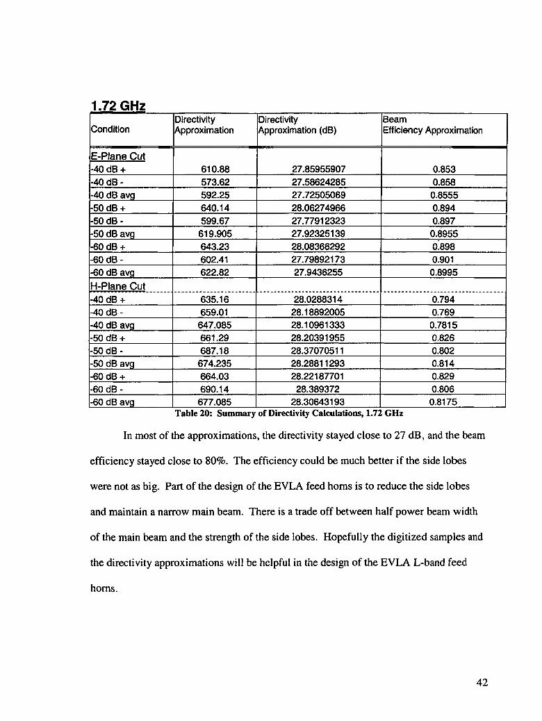
1.72 GHzCondition
DirectivityApproximation
Directivity Approximation (dB)
BeamEfficiency Approximation
E-Plane Cut610.88 27.85955907 0.853-40 dB +
-40 dB - 573.62 27.58624285 0.858-40 dB avg 592.25 27.72505069 0.8555-50 dB + 640.14 28.06274966 0.894-50 dB - 599.67 27.77912323 0.897-50 dB avg 619.905 27.92325139 0.8955-60 dB + 643.23 28.08366292 0.898-60 dB - 602.41 27.79892173 0.901-60 dB avg 622.82 27.9436255 0.8995H-Plane Cut-40 dB + 635.16 28.0288314 0.794-40 dB - 659.01 28.18892005 0.769-40 dB avg 647.085 28.10961333 0.7815-50 dB + 661.29 28.20391955 0.826-50 dB - 687.18 28.37070511 0.802-50 dB avg 674.235 28.28811293 0.814-60 dB + 664.03 28.22187701 0.829-60 dB - 690.14 28.389372 0.806-60 dB avg 677.085 28.30643193 0.8175
Table 20: Summary of Directivity Calculations, 1.72 GHz
In most of the approximations, the directivity stayed close to 27 dB, and the beam
efficiency stayed close to 80%. The efficiency could be much better if the side lobes
were not as big. Part of the design of the EVLA feed horns is to reduce the side lobes
and maintain a narrow main beam. There is a trade off between half power beam width
of the main beam and the strength of the side lobes. Hopefully the digitized samples and
the directivity approximations will be helpful in the design of the EVLA L-band feed
horns.
42

APPENDIX A
APPENDIX A: EMS Path and Antenna Characteristics
Injected Signal Power: -60 dBm Data obtained by Eric Reynolds and Raul Armendariz, 8/14/01
Band(in FE)
InjectedSignal
(frequency)
MeasuredOutput(dBm)
Measured Net Gain
(dB)
Theoretical Net Gain
(1) - (2) - (3)DifferenceTHE - MEA
Band 1 20 MHz -51 9 11 - .3 - .05 = 10.7 1.7200 MHz -50 10 11 -1 .0 -.17 = 9.8 -0.2
P-Band 400 MHz -51 9 11 -1.5 - .24 = 9.3 0.3Low 600 MHz -51 9 11 -1.8 - .29 = 8.9 -0.1
Gain 800 MHz -51 9 11-2.1 - .35 = 8.6 -0.41000 MHz -51 9 11 - 2.4 - .39 = 8.2 -0.8
Band 2 100 MHz -27 33 34 - .3 - .05 = 33.7 0.7200 MHz -27 33 34 -1 .0 -.17 = 32.8 -0.2
P-Band 400 MHz -28 32 34 -1 .5 -.24 = 32.3 0.3High 600 MHz -28 32 34 -1 .8 -.29 = 31.9 -0.1Gain 800 MHz -28 32 34-2.1 - .35 = 31.6 -0.4
1000 MHz -28 32 34 -2 .4 -.39 = 31.2 -0.8Band 3 1 GHz -59 1 3 .8 -2 .4 -.39 = 1.0 0
1.2 GHz -55 5 7.2 - 2.7 - .44 = 4.1 -0.9L-Band 1.4 GHz -55 5 7.2 - 2.9 - .47 = 3.8 -1.2
Low 1.6 GHz -57 3 7.2 - 3.1 - .51 = 3.6 0.6Gain 1.8 GHz -58 2 7.2 - 3.3 - .55 = 3.4 1.4
2 GHz -59 1 5.1 -3 .5 -.57 = 3.1 2.1Band 4 1 GHz -64 -4 -2.4 - 2.4 - .39 = -5.2 -1.2
1.2 GHz -45 15 20-2.7- .44 = 16.9 1.9L-Band 1.4 GHz -28 32 34 - 2.9 - .47 = 30.6 -1.4
High 1.6 GHz -30 30 34 - 3.1 - .51 = 30.4 0.4Gain 1.8 GHz -31 29 34 - 3.3 - .55 = 30.2 1.2
2 GHz -71 -11 -6.7-3.5-.57 = -10.8 0.2Band5 2 GHz -34 26 30 - 3.5 - .57 = 25.9 -0.1
2.2 GHz -35 25 30 - 3.6 - .61 = 25.8 0.82.4 GHz -35 25 30 - 3.8 - .63 = 25.6 0.6
S-Band 2.6 GHz -35 25 30 - 3.9 - .66 = 25.4 0.42.8 GHz -34 26 30 - 4.1 - .69 = 25.2 -0.83 GHz -36 24 30 - 4.4 - .72 = 24.9 0.9
3.2 GHz -37 23 30 - 4.5 - .75 = 24.8 1.83.4 GHz -36 24 30 - 4.7 - .77 = 24.5 0.53.6 GHz -36 24 30 - 4.8 - .80 = 24.4 0.43.8 GHz -37 23 30 - 4.9 - .83 = 24.3 1.34 GHz -38 22 30 - 5.2 - .85 = 23.9 1.9
43

Band 6 4 GHz -32 28 35 - 5.2 - .85 = 28.9 0.9
4.5 GHz
COCO1 27 35-5 .6 - .91 =28.5 1.55 GHz -33 27 35 -5 .9 - .9 7 = 28.1 1.1
5.5 GHz -35 25 35-6.3-1 .03 = 27.7 2.76 GHz -36 24 33-6.6-1 .08 = 25.3 1.3
C-Band 6.5 GHz -36 24 33-6.9-1.14 = 24.9 0.97 GHz -37 23 33-7.3-1 .19 = 24.5 1.5
7.5 GHz -37 23 33-7.6-1 .25 = 24.2 1.28 GHz -37 23 35-7.9-1 .29 = 25.8 2.8
8.5 GHz -37 23 33-8.2-1 .34 = 23.5 0.59 GHz -38 22 32-8.5-1.39 = 22.1 0.1
9.5 GHz -39 21 32-8.8-1 .44 = 21.8 0.810 GHz -41 19 32-9.1 -1.49 = 21.4 2.4
Band 7 10 GHz -77 -17 0 1 CD 1 CO II i u o b) 6.411 GHz -78 -18 0 - 9.6 -1.57 = -11.2 5.812 GHz -78 -18 0-10.2 - 1.67 = -11.9 6.113 GHz
o00• oCM• 0 1 0
■ ____
___k
■nJ 01
II ■ ro cn 7.5X-Band 14 GHz -79 -19
15 GHzo001 -20
16 GHz -85 -2517 GHz -85 -2518 GHz -86 -26
44
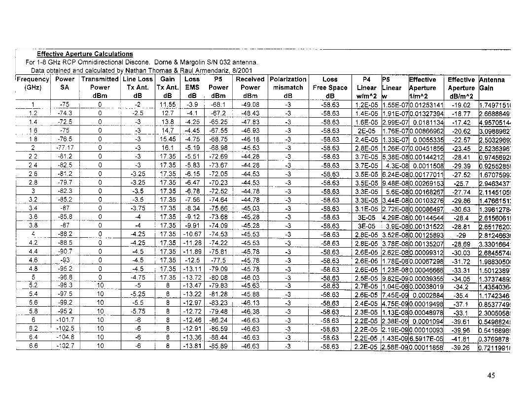
Effective Aperture CalculationsFor 1-8 GHz RCP Omnidirectional Discone. Dome & Margolin S/N 032 antenna.
Data obtained and calculated by Nathan Thomas & Raul Armendariz, 8/2001Frequency
(GHz)Power
SATransmitted
PowerdBm
Line Loss Tx Ant.
dB
Gain Tx Ant.
dB
LossEMSdB
P5PowerdBm
ReceivedPowerdBm
Polarizationmismatch
dB
Loss Free Space
dB
P4Linearw/mA2
P5Linearw
EffectiveAperture1/mA2
EffectiveAperturedB/mA2
AntennaGain
1 -75 0 -2 11.55 -3.9 -68.1 -49.08 -3 -58.63 1.2E-05 1.55E-07 0.01253141 -19.02 1.749715111.2 -74.3 0 -2.5 12.7 -4.1 -67.2 -48.43 -3 -58.63 1.4E-05 1.91E-07 0.01327394 -18.77 2.66888491.4 -72.5 0 -3 13.8 -4.25 -65.25 -47.83 -3 -58.63 1.6E-05 2.99E-07 0.0181134 -17.42 4.9570514'1.6 -75 0 -3 14.7 -4.45 -67.55 -46.93 -3 -58.63 2E-05 1.76E-07 0.00866962 -20.62 3.0988982'1.8 -76.5 0 -3 15.45 -4.75 -68.75 -46.18 -3 -58.63 2.4E-05 1.33E-07 0.0055335 -22.57 2.5032969:2 -77.17 0 -3 16.1 -5.19 -68.98 -45.53 -3 -58.63 2.8E-05 1.26E-07 0.00451856 -23.45 2.5236396'
2.2 -81.2 0 -3 17.35 -5.51 -72.69 -44.28 -3 -58.63 3.7E-05 5.38E-08 0.00144212 -28.41 0.9745692I2.4 -82.5 0 -3 17.35 -5.83 -73.67 -44.28 -3 -58.63 3.7E-05 4.3E-08 0.0011508 -29.39 0.9255285!2.6 -81.2 0 -3.25 17.35 -6.15 -72.05 -44.53 -3 -58.63 3.5E-05 6.24E-08 0.00177011 -27.52 1.6707599:2.8 -79.7 0 -3.25 17.35 -6.47 -70.23 -44.53 -3 -58.63 3.5E-05 9.48E-08 0.00269153 -25.7 2.9463437'3 -82.3 0 -3.5 17.35 -6.78 -72.52 -44.78 -3 -58.63 3.3E-05 5.6E-08 0.00168267 -27.74 2.1145105!
3.2 -85.2 0 -3.5 17.35 -7.56 -74.64 -44.78 -3 -58.63 3.3E-05 3.44E-08 0.00103276 -29.86 1.4766151:3.4 -87 0 -3.75 17.35 -8.34 -75.66 -45.03 -3 -58.63 3.1E-05 2.72E-08 0.00086497 -30.63 1.3961278-3.6 -85.8 0 -4 17.35 -9.12 -73.68 -45.28 -3 -58.63 3E-05 4.29E-08 0.00144544 -28.4 2.6156061!3.8 -87 0 -4 17.35 -9.91 -74.09 -45.28 -3 -58.63 3E-05 3.9E-08 0.00131522 -28.81 2.6517620:4 -88.2 0 -4.25 17.35 -10.67 -74.53 -45.53 -3 -58.63 2.8E-05 3.52E-08 0.00125893 -29 2.8124663(
4.2 -88.5 0 -4.25 17.35 -11.28 -74.22 -45.53 -3 -58.63 2.8E-05 3.78E-08 0.00135207 -28.69 3.3301664'4.4 -90.7 0 -4.5 17.35 -11.89 -75.81 -45.78 -3 -58.63 2.6E-05 2.62E-08 0.00099312 -30.03 2.6845574I4.6 -93 0 -4.5 17.35 -12.5 -77.5 -45.78 -3 -58.63 2.6E-05 1.78E-08 0.00067298 -31.72 1.988305014.8 -95.2 0 -4.5 17.35 -13.11 -79.09 -45.78 -3 -58.63 2.6E-05 1.23E-08 0.00046666 -33.31 1.5012389'5 -96.8 0 -4.75 17.35 -13.72 -80.08 -46.03 -3 -58.63 2.5E-05 9.82E-09 0.00039355 -34.05 1.3737489:
5.2 -96.3 10 -5 8 -13.47 -79.83 -45.63 -3 -58.63 2.7E-05 1.04E-08 0.00038019 -34.2 1.4354036-5.4 -97.5 10 -5.25 8 -13.22 -81.28 -45.88 -3 -58.63 2.6E-05 7.45E-09 0.0002884 -35.4 1.17423465.6 -99.2 10 -5.5 8 -12.97 -83.23 -46.13 -3 -58.63 2.4E-05 4.75E-09 0.00019498 -37.1 0.8537749!5.8 -95.2 10 -5.75 8 -12.72 -79.48 -46.38 -3 -58.63 2.3E-05 1.13E-08 0.00048978 -33.1 2.3005058!6 -101.7 10 -6 8 -12.46 -86.24 -46.63 -3 -58.63 2.2E-05 2.38E-09 0.0001094 -39.61 0.5498824!
6.2 -102.5 10 -6 8 -12.91 -86.59 -46.63 -3 -58.63 2.2E-05 2.19E-09 0.00010093 -39.96 0.5416898!6.4 -104.8 10 -6 8 -13.36 -88.44 -46.63 -3 -58.63 2.2E-05 1.43E-09 6.5917E-05 -41.81 0.37698786.6 -102.7 10 -6 8 -13.81 -85.89 -46.63 -3 -58.63 2.2E-05 2.58E-09 0.00011858 -39.26 0.72119911
45


6.8 -105.7 10 -6 8 -14.26 -88.44 -46.63 -3 -58.63 2.2E-05 1.43E-09 6.5917E-05 -41.81 0.4255838!7 -105.8 10 -6.5 8 -14.72 -88.08 -47.13 -3 -58.63 1.9E-05 1.56E-09 8.0353E-05 -40.95 0.5497477!
7.2 -103.2 10 -6.5 8 -14.76 -85.44 -47.13 -3 -58.63 1.9E-05 2.86E-09 0.00014757 -38.31 1.0681502!7.4 -103.2 10 -6.75 8 -14.8 -85.4 -47.38 -3 -58.63 1.8E-05 2.88E-09 0.00015776 -38.02 1.2062318(7.6 -102.3 10 -7 8 -14.84 -84.46 -47.63 -3 -58.63 1.7E-05 3.58E-09 0.00020749 -36.83 1.6733798'7.8 -103.5 10 -7 8 -14.88 -85.62 -47.63 -3 -58.63 1.7E-05 2.74E-09 0.00015885 -37.99 1.3494492(8 -104.2 10 -7.25 8 -14.91 -86.29 -47.88 -3 -58.63 1.6E-05 2.35E-09 0.00014421 -38.41 1.2886866!
46


47


APPENDIX B: List of References and Sources
Spectrum Guide. Frequency Allocations in the United States. 30 MHz - 300GHz Bennet Z. KobbThird Edition, New Signals Press, 1996
Antennas John D. Kraus2nd Edition, McGraw-Hill, 1988
Measuring the Radio Frequency EnvironmentE. Skomal & A. SmithVon Nonstrand Reinhold Company, 1985
Spectrum Monitoring Handbook International Telecommunications Union, 1995
48