evolution leads to kantian morality
TRANSCRIPT
Evolution leads to Kantian morality∗
Ingela Alger† and Jörgen W. Weibull‡
June 3, 2015
Abstract
What preferences or moral values should one expect evolution to favor? We provide
a generalized definition of evolutionary stability of heritable traits in arbitrarily large
aggregative interactions under random matching that may be assortative. We establish
stability results when these traits are strategies in games, and when they are preferences
or moral values in games in which each player’s preferences or moral values are the
player’s private information. We show that certain moral preferences, of a kind that
exactly reflects the assortativity in the matching process, are evolutionarily stable. In
particular, selfishness is evolutionarily unstable as soon as there is any assortativity.
We also establish that evolutionarily stable strategies are the same as those played
in equilibrium by rational individuals with evolutionarily stable moral preferences.
We provide simple operational criteria for evolutionary stability and apply these to
canonical examples.
Keywords: Evolutionary stability, assortativity, morality, homo moralis, public
goods, contests, helping.
JEL codes: C73, D01, D03.
∗Support by Knut and Alice Wallenberg Research Foundation and by ANR - Labex IAST is gratefully
acknowledged. Ingela Alger also thanks Agence Nationale de la Recherche (ANR) for funding (Chaire
d’Excellence). We are grateful for comments from seminar participants at EconomiX, WZB, GREQAM,
ETH Zürich, Nottingham, OECD, Séminaire Roy (PSE), IGIER Bocconi, Bern, and École Polytechnique,
and from participants at the 2nd Toulouse Economics and Biology Workshop, the 2014 EEA meeting, and
the 2014 ASSET meeting.
†Toulouse School of Economics (LERNA, CNRS) and Institute for Advanced Study in Toulouse
‡Stockholm School of Economics, KTH Royal Institute of Technology, and Institute for Advanced Study
in Toulouse
1
1 Introduction
Economics provides a rich set of powerful theoretical models of human societies. Since these
models feature individuals whose motivations–preferences and/or moral values–are given,
their predictive power depends on the assumptions made regarding these motivations. But if
preferences are inherited from past generations, the formation of these preferences may itself
be studied theoretically. In particular, one may ask what preferences or moral values have
a survival value, and thus what preferences and moral values humans should be expected to
have from first principles.
Should we expect pure self-interest, altruism (Becker, 1976), warm glow (Andreoni, 1990),
reciprocal altruism (Levine, 1998), inequity aversion (Fehr and Schmidt, 1999), self-image
concerns (Bénabou and Tirole, 2006), moral motivation (Brekke, Kverndokk, and Nyborg,
2003), or something else? This question is at the heart of the literature on preference
evolution initiated by Güth and Yaari (1992). In a recent contribution to this literature,
we found that evolution under certain conditions favors a class of preferences that we called
homo moralis (Alger andWeibull, 2013).1 We derived this result in a model where individuals
interact in pairs. Homo moralis then attaches some weight to his material self-interest but
also to what is “the right thing to do if others would do what I do”. But in real life
many interactions involve more than two persons. Can the methods and results for pairwise
interactions be generalized, and if so, how? What preferences and/or moral values does
evolution lead to then? These are the questions we address in this paper.
Two major issues drive this quest. First, since (to the best of our knowledge) this
exploration has not been made before, we simply did not know what preferences to find. Like
in Alger and Weibull (2013), we will let the mathematics show us the way to the preferences
that evolution favors, but now for groups of arbitrary size. Our finding, arguably not easy
to anticipate and expressing a form of social preference-cum-morality that we have not seen
before, will be reported and examined here. The second major reason for pursuing this work
is to find out whether moral motivation is evolutionarily viable only in small groups.
More precisely, we propose a general model for the study of the evolutionary founda-
tions of human motivation in strategic interactions in arbitrarily large groups. We define
evolutionary stability as a property of abstract “traits” or “types” that can be virtually
any characteristic of an individual, such as a behavior pattern or strategy, a goal function,
1See also the discussion in Bergstrom (1995).
2
preference, moral value, belief, or cognitive capacity. Individuals live in a infinite population
and are randomly matched in groups of size to play an -player game. Each player gets a
material payoff that depends on his or her own strategy and on some aggregate of the others’
strategies; formally, individuals play an aggregative game in material payoffs.2 Each player’s
strategy set may be simple, such as in a simultaneous-move game, or very complex, such as
in a extensive-form game with many information sets. Strategies may be pure or mixed. A
type is evolutionarily stable if it materially outperforms other types, when the latter appear
as rare mutants in the population, and a type is evolutionarily unstable if it is materially
outperformed by some rare mutant type.
A key assumption in our model is that the random matching may be assortative in the
sense that individuals who are of a vanishingly rare (“mutant”) type may face a positive
probability of being matched with others of their own rare type, even in the limit as the rare
type vanishes. While such matching patterns may at first appear counter-intuitive or even
impossible, it is not difficult to think of reasons for why they can arise. First, while distance is
not explicitly modeled here, geographic, cultural, linguistic and socioeconomic space imposes
(literal or metaphoric) transportation costs, which imply that (1) individuals tend to interact
more with individuals in their (geographic, cultural, linguistic or socioeconomic) vicinity,3
and (2) cultural or genetic transmission of types (say, behavior patterns, preferences or
moral values) from one generation to the next also has a natural tendency to take place in
the vicinity of where the rare type originally appeared. Taken together, these two tendencies
imply the assortativity that we here allow for.4 In the present model we formalize the
2The notion of aggregative games is, to the best of our knowledge, due to Dubey, Mas-Colell and Shubik
(1980). See also Corchón (1996). The key feature is that the payoff to a player depends only on the players’
own strategy and some (symmetric) aggregation of others’ strategies. For a recent paper on aggregative
games, see Acemoglu and Jensen (2013). For work on aggregative games more related to ours, see Haigh and
Cannings (1989) and Koçkesen, Ok and Sethi (2000a,b).
3Homophily has been documented by sociologists (e.g., McPherson, Smith-Lovin, and Cook, 2001, and
Ruef, Aldrich, and Carter, 2003) and economists (e.g., Currarini, Jackson, and Pin, 2009, 2010, and Bra-
moullé and Rogers, 2009). In particular, in a study about race and gender-based choice of friends and meeting
chances in U.S. high schools, Currarini, Jackson, and Pin (2009) find that there are strong within-group bi-
ases not only in the inferred utility from meetings but also in meeting probabilities. This is particularly
relevant for us, since we assume away partner choice.
4In biology, the concept of assortativity is known as relatedness, and the propensity to interact with
individuals locally is nicely captured in the infinite island model, originally due to Wright (1931); see also
Rousset (2004).
3
assortativity of a random matching process in terms of what we call the assortativity profile;
a probability vector for the events that none, some, or all the individuals in a (vanishingly
rare) mutant’s group also are mutants, thus generalizing Bergstrom’s (2003) definition of
assortativity from pairwise encounters to -person encounters.5
Our analysis delivers three main results. First, although we impose minimal restrictions
on potential preferences or moral values, our analysis, when applied to preference evolution
under incomplete information shows that evolution favors a particular class of preferences.
An individual with preferences in this class evaluates what would happen to her own mate-
rial payoff if with some probability others were to do as she does. Such preferences allow a
distinct moral interpretation, and accordingly we use the name homo moralis for this class
of preferences.6 In particular they generalize Kantian morality in a probabilistic direction.
Indeed, in his Grundlegung zür Metaphysik der Sitten (1785), Immanuel Kant wrote “Act
only according to that maxim whereby you can, at the same time, will that it should be-
come a universal law.” Similarly, homo moralis can be interpreted to “act according to that
maxim whereby you can, at the same time, will that others should do likewise with some
probability.”7
Importantly, homo moralis preferences for groups of size above two are qualitatively
different from those for groups of size two. For arbitrary group size , a homo moralis
individual maximizes a weighted average of terms, where the term, for = 1 2 , is
the (hypothetical) material payoff that the individual would obtain if −1 other individualswould use the same strategy as the individual uses. For evolutionary stability the weights
must exactly reflect the assortativity profile. Furthermore, and this is the second main
result, any preferences that lead to equilibrium behaviors that differ from those of homo
moralis are evolutionarily unstable. In particular, then, our results imply that material self-
interest is evolutionarily inviable as soon as the probability is positive that at least one of the
individuals with whom a mutant interacts also is a mutant (when mutants are vanishingly
rare).
Our third main result is that the equilibrium behaviors among homo moralis whose
morality profile exactly reflects the assortativity profile are the same as the behaviors selected
5See Bergstrom (2013) and Alger and Weibull (2013) for further discussions of assortativity when = 2.
6For a discussion of several ethical principles, see Bergstrom (2009).
7Homo moralis preferences have got nothing to do with the equilibrium concept “Kantian equilibrium”
proposed by Roemer (2010).
4
for under strategy evolution. This result establishes that evolutionarily stable strategies
(under uniform or assortative random matching) need not be interpreted only as resulting
when individuals are “programmed” to certain strategies, but can also be interpreted as
resulting when individual are rational and free to choose whatever strategy they like, but
whose preferences have emerged from natural selection. Together with a first- and second-
order characterization for games in Euclidean strategy spaces under conditional independence
in the assortativity, we obtain operational methods to find the (symmetric) equilibria of -
player games among homo moralis, methods we illustrate in various canonical examples.
The general model is described in the next section. This model is then applied to prefer-
ence evolution under incomplete information (Section 3) and strategy evolution (Section 4).
In Section 5 we present a characterization result, which we then apply to several commonly
studied games in Section 6. Prior to concluding (Section 8), we review the literature in
Section 7.
2 Model
Consider an infinite (continuum) population of individuals who are randomly matched into
groups of ≥ 1 individuals to interact according to some game given in normal form Γ =
h i, where = 1 2 is the set of players, is the set of strategies available
to each player and : ×−1 → R is the material payoff function.8 The material payoff
to any player ∈ from using strategy ∈ against the strategies ∈ ( 6= ) of
the others in the group is denoted (x−). We assume that (x−) is invariant under
permutations of the components of x−, the strategy profile of all other individuals in the
group. These games may thus be called aggregative.9 We will assume throughout that the
set is a non-empty, compact and convex set in some topological vector space, and that the
function is continuous.10 The generality of the strategy set allows for simultaneous-move
8This game will subsequently serve as a “game protocol” in the sense of Weibull (2004), that is, partici-
pants will be allowed to have their own personal preferences over strategy profiles, preferences that are not
required to be functions of the material payoff outcomes.
9More precisely: for any ∈ and x− ∈ −1, and any bijection : 2 3 → 2 3 :¡ (2) (3) ()
¢= (x−).
10More precisely, it is sufficient for the subsequant analysis that is a locally convex Hausdorff space, see
Aliprantis and Border (2006).
5
games, games with sequential moves and asymmetric information etc. Indeed, Γ may be any
symmetric and finite -player extensive-form game with perfect recall and its the set of
mixed or behavior strategies.
Each individual has some type (or trait) ∈ Θ, which may influence his/her choice of
strategy, or behavior in the game Γ, where Θ is the set of potential types. Consider a
population in which at most two types from Θ are present. For any types and , and any
∈ (0 1), let = ( ) be the population state in which the two types are represented inpopulation shares 1− and , respectively. Let = Θ2× (0 1) denote the set of populationstates. We are particularly interested in states = ( ) in which is small, then calling
the resident type, being predominant in the population, and , being rare, the mutant type.
In a given population state ∈ , the behavioral outcomes, or, more precisely, strategy
profiles used, may, but need not, be uniquely determined. For each population state , let
() ⊂ R2 be the set of (average) material-payoff pairs that can arise in population state, where, for any = (1 2) ∈ ( ), the first component, 1, is the average material
payoff to individuals of type , and the second component, 2, that to individuals of type .
We assume that () is non-empty and compact for all states = ( ). Then
( ) = min∈ ( )
(1 − 2) (1)
is well-defined. In words, ( ), is the material payoff difference between residents and
mutants, in the residents’ worst possible outcome as compared with mutants (in terms of
material payoffs), across all behavioral outcomes that are possible in state = ( ). In
particular, () 0 if and only if the residents earn a (strictly) higher (average) material
payoff than the mutants in all possible outcomes in that state.11
The following definitions of evolutionary stability and instability are generalizations of
the definitions in Alger and Weibull (2013), from = 2 to ≥ 2, and from preferences to
arbitrary types.
Definition 1 A type is evolutionarily stable against a type if ( ) 0 for
all 0 sufficiently small. A type is evolutionarily stable if it is evolutionarily stable
against all types 6= . A type is evolutionarily unstable if there exists a type such
that ( ) 0 for arbitrarily small 0.
11The function is a generalization of the so-called score function in evolutionary game theory, see, e.g.,
Bomze and Pötscher (1989).
6
Our requirement for stability is demanding; the residents should earn a higher material
payoff in all behavioral outcomes for all sufficiently small population shares of the mutant
type. By contrast, the requirement for instability is relatively weak; it suffices to find one
type that would earn a higher material payoff in some behavioral outcome in some pop-
ulation state with arbitrarily few mutants.12 Clearly, by these definitions no type is both
evolutionarily stable and unstable, and there may, in general, exist types that are neither
stable nor unstable.
2.1 Matching
The matching process is exogenous. In any population state = ( ) ∈ , the number
of mutants–individuals of type –in a group that is about to play game Γ = h i,is a random variable that we will denote . For any resident drawn at random from the
population let () be the conditional probability Pr [ = | ] that the total numberof mutants in the resident’s group is , for = 0 1 − 1.13 Likewise, for any mu-
tant, also drawn at random from the population, let () be the conditional probability
Pr [ = | ] that the total number of mutants in his or her group is , for = 1 .
We assume that each function and each function is continuous and has a limit as
→ 0, which we denote 0 and 0, respectively.
In order to get a grip on these limiting probabilities, we use the algebra of assortative
encounters developed by Bergstrom (2003) for pairwise interactions. For a given population
state = ( ), let Pr [| ] denote the conditional probability for an individual of type that another, uniformly randomly drawn member of his or her group also is of type .
Likewise, let Pr [| ] denote the conditional probability for an individual of type thatany other uniformly randomly drawn member of his or her group has type . Let () be
the difference between the two probabilities:
() = Pr [| ]− Pr [| ] (2)
12More precisely, for any given 0 there should exist some 0 ∈ (0 ) such that ( 0) 0.13The first random draw cannot, technically, be uniform, in an infinite population. The reasoning in this
section is concerned with matchings in finite populations in the limit as the total population size goes to
infinity. We refer the reader to the appendix for a detailed example.
7
This defines the assortment function : (0 1)→ [−1 1]. We assume that
lim→0
() = (3)
for some ∈ R, the index of assortativity of the matching process (Bergstrom, 2003).
Moreover, by setting (0) = we henceforth extend the domain of from (0 1) to [0 1).
The following equation is a necessary balancing condition:
(1− ) · [1− Pr [| ]] = · Pr [| ] (4)
Each side of the equation equals the probability for the following event: draw at random an
individual from the population at large and then draw at random another individual from
the first individual’s group, and observe that these two individuals are of different types.
Equations (2) and (4) together give(Pr [| ] = () + (1− ) [1− ()]
Pr [| ] = (1− ) [1− ()] (5)
Now let → 0. Then, from (4), Pr [| ] → 1, and hence 0 () → 1. In other words,
residents virtually never meet mutants when the latter are vanishingly rare. Without loss
of generality we may thus uniquely extend the domain of from (0 1) to [0 1), while
preserving its continuity, by setting 0 (0) = 1. We also note that together with (5), this
property implies that ∈ [0 1].14
Turning now to the limit of () as tends to zero (for = 1 ), we first note that
in the special case = 2,
02 = lim→0
Pr [ | ] = 1− lim→0
Pr [| ] = 1−h1− lim
→0 ()
i=
However, for 2 there remains a statistical issue, namely whether or not, for a given
mutant, the types of any two other members in her group are statistically dependent or not
(in the given population state). We will not make any specific assumption about this in the
general analysis, and we will refer to the vector q0 = (01 0) as the assortativity profile
of the matching process.
14This contrasts with the case of a finite population, where negative assortativity can arise for population
states with few mutants (see Schaffer, 1988).
8
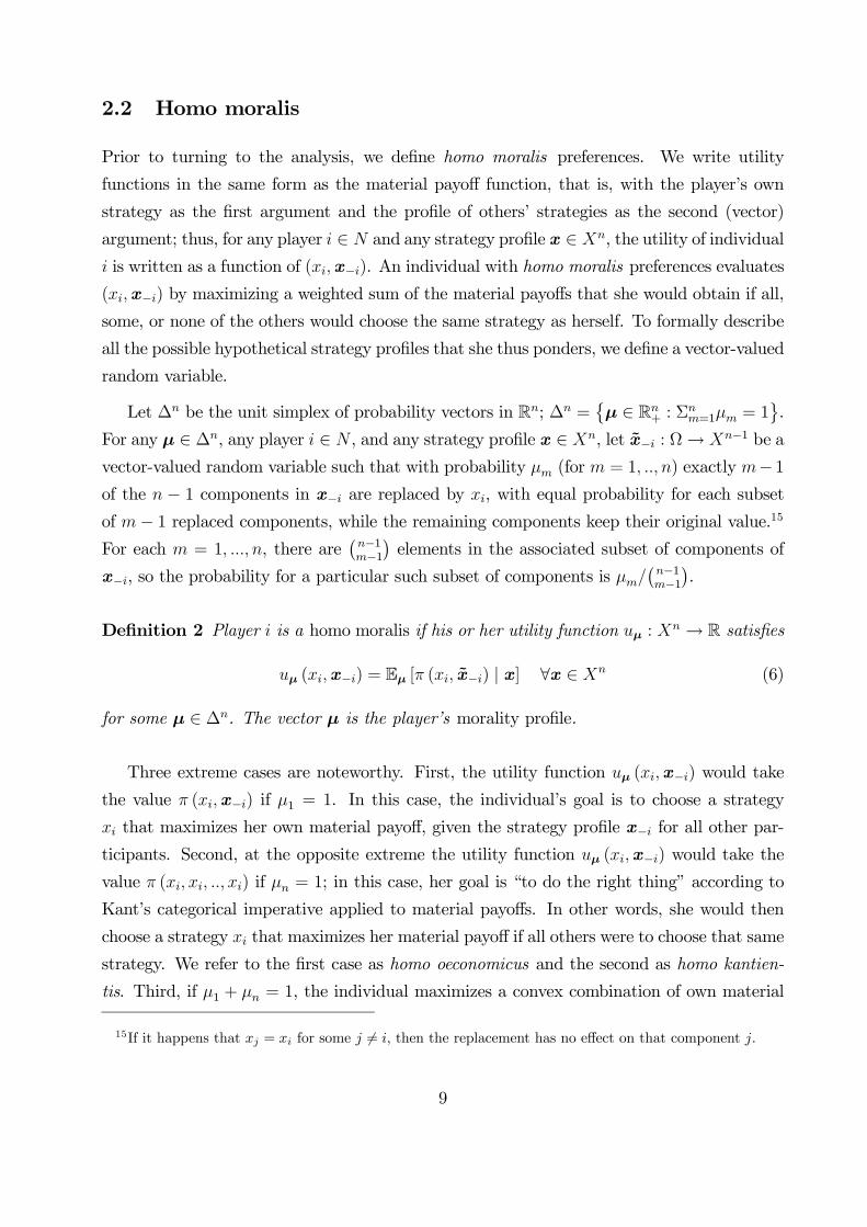
2.2 Homo moralis
Prior to turning to the analysis, we define homo moralis preferences. We write utility
functions in the same form as the material payoff function, that is, with the player’s own
strategy as the first argument and the profile of others’ strategies as the second (vector)
argument; thus, for any player ∈ and any strategy profile x ∈ , the utility of individual
is written as a function of (x−). An individual with homo moralis preferences evaluates
(x−) by maximizing a weighted sum of the material payoffs that she would obtain if all,
some, or none of the others would choose the same strategy as herself. To formally describe
all the possible hypothetical strategy profiles that she thus ponders, we define a vector-valued
random variable.
Let ∆ be the unit simplex of probability vectors in R; ∆ =©μ ∈ R
+ : Σ=1 = 1
ª.
For any μ ∈ ∆, any player ∈ , and any strategy profile x ∈ , let x− : Ω→ −1 be a
vector-valued random variable such that with probability (for = 1 ) exactly − 1of the − 1 components in x− are replaced by , with equal probability for each subset
of − 1 replaced components, while the remaining components keep their original value.15For each = 1 , there are
¡−1−1
¢elements in the associated subset of components of
x−, so the probability for a particular such subset of components is ¡−1−1
¢.
Definition 2 Player is a homo moralis if his or her utility function : → R satisfies
(x−) = E [ ( x−) | x] ∀x ∈ (6)
for some μ ∈ ∆. The vector μ is the player’s morality profile.
Three extreme cases are noteworthy. First, the utility function (x−) would take
the value (x−) if 1 = 1. In this case, the individual’s goal is to choose a strategy
that maximizes her own material payoff, given the strategy profile x− for all other par-
ticipants. Second, at the opposite extreme the utility function (x−) would take the
value ( ) if = 1; in this case, her goal is “to do the right thing” according to
Kant’s categorical imperative applied to material payoffs. In other words, she would then
choose a strategy that maximizes her material payoff if all others were to choose that same
strategy. We refer to the first case as homo oeconomicus and the second as homo kantien-
tis. Third, if 1 + = 1, the individual maximizes a convex combination of own material
15If it happens that = for some 6= , then the replacement has no effect on that component .
9
payoff and the material payoff that would arise should all players use the same strategy
: (x−) = 1 · (x−) + · ( ). In particular, if = 2 the equality1 + = 1 always holds and one then obtains ( ) = (1− ) · ( ) + · ( ) for = 2, the same expression as in Alger and Weibull (2013). However, for 2 a homo
moralis may also attach a positive weight to the material payoff that she would obtain if
some but not all others were to use the same strategy as herself. Morality still has a distinct
Kantian flavor, since the individual evaluates what would happen to her material payoff if
others were to behave as she does.
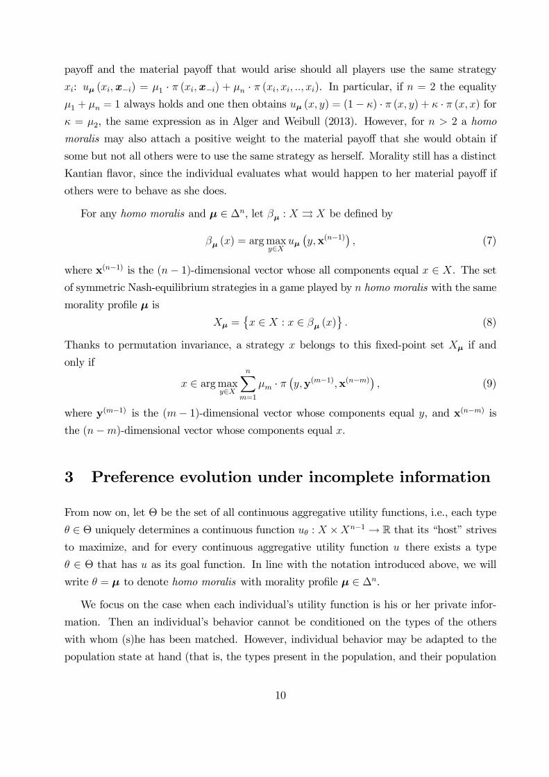
For any homo moralis and μ ∈ ∆, let : ⇒ be defined by
() = argmax∈
¡x(−1)
¢ (7)
where x(−1) is the (− 1)-dimensional vector whose all components equal ∈ . The set
of symmetric Nash-equilibrium strategies in a game played by homo moralis with the same
morality profile μ is
=© ∈ : ∈ ()
ª (8)
Thanks to permutation invariance, a strategy belongs to this fixed-point set if and
only if
∈ argmax∈
X=1
· ¡y(−1)x(−)
¢ (9)
where y(−1) is the (− 1)-dimensional vector whose components equal , and x(−) isthe (−)-dimensional vector whose components equal .
3 Preference evolution under incomplete information
From now on, let Θ be the set of all continuous aggregative utility functions, i.e., each type
∈ Θ uniquely determines a continuous function : ×−1 → R that its “host” strives
to maximize, and for every continuous aggregative utility function there exists a type
∈ Θ that has as its goal function. In line with the notation introduced above, we will
write = μ to denote homo moralis with morality profile μ ∈ ∆.
We focus on the case when each individual’s utility function is his or her private infor-
mation. Then an individual’s behavior cannot be conditioned on the types of the others
with whom (s)he has been matched. However, individual behavior may be adapted to the
population state at hand (that is, the types present in the population, and their population
10
shares). Arguably, Bayesian Nash equilibrium is a natural criterion to delineate the set ()
of (average) material-payoff pairs that can arise in a population state .16
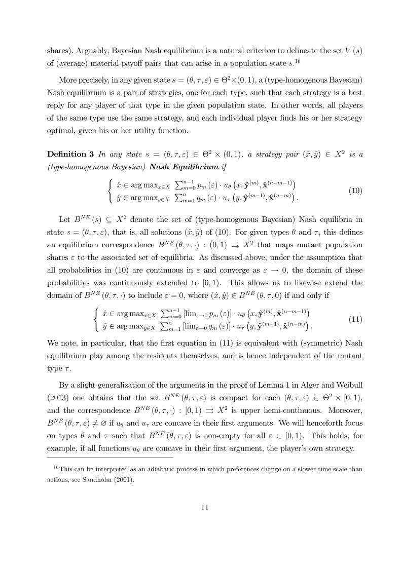
More precisely, in any given state = ( ) ∈ Θ2×(0 1), a (type-homogenous Bayesian)Nash equilibrium is a pair of strategies, one for each type, such that each strategy is a best
reply for any player of that type in the given population state. In other words, all players
of the same type use the same strategy, and each individual player finds his or her strategy
optimal, given his or her utility function.
Definition 3 In any state = ( ) ∈ Θ2 × (0 1), a strategy pair ( ) ∈ 2 is a
(type-homogenous Bayesian) Nash Equilibrium if( ∈ argmax∈
P−1=0 () ·
¡ y() x(−−1)
¢ ∈ argmax∈
P
=1 () · ¡ y(−1) x(−)
¢
(10)
Let () ⊆ 2 denote the set of (type-homogenous Bayesian) Nash equilibria in
state = ( ), that is, all solutions ( ) of (10). For given types and , this defines
an equilibrium correspondence ( ·) : (0 1) ⇒ 2 that maps mutant population
shares to the associated set of equilibria. As discussed above, under the assumption that
all probabilities in (10) are continuous in and converge as → 0, the domain of these
probabilities was continuously extended to [0 1). This allows us to likewise extend the
domain of ( ·) to include = 0, where ( ) ∈ ( 0) if and only if( ∈ argmax∈
P−1=0 [lim→0 ()] ·
¡ y() x(−−1)
¢ ∈ argmax∈
P
=1 [lim→0 ()] · ¡ y(−1) x(−)
¢
(11)
We note, in particular, that the first equation in (11) is equivalent with (symmetric) Nash
equilibrium play among the residents themselves, and is hence independent of the mutant
type .
By a slight generalization of the arguments in the proof of Lemma 1 in Alger and Weibull
(2013) one obtains that the set ( ) is compact for each ( ) ∈ Θ2 × [0 1),and the correspondence ( ·) : [0 1) ⇒ 2 is upper hemi-continuous. Moreover,
( ) 6= ∅ if and are concave in their first arguments. We will henceforth focuson types and such that ( ) is non-empty for all ∈ [0 1). This holds, forexample, if all functions are concave in their first argument, the player’s own strategy.
16This can be interpreted as an adiabatic process in which preferences change on a slower time scale than
actions, see Sandholm (2001).
11
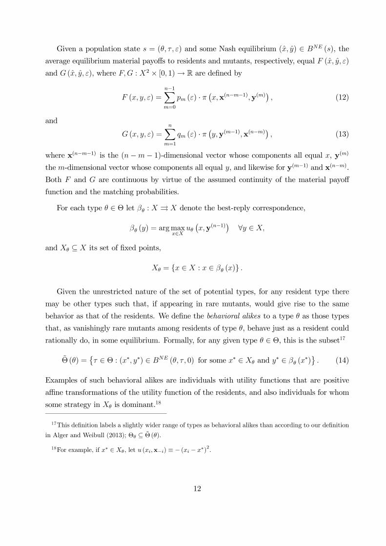
Given a population state = ( ) and some Nash equilibrium ( ) ∈ (), the
average equilibrium material payoffs to residents and mutants, respectively, equal ( )
and ( ), where : 2 × [0 1)→ R are defined by
( ) =
−1X=0
() · ¡x(−−1)y()
¢ (12)
and
( ) =
X=1
() · ¡y(−1)x(−)
¢ (13)
where x(−−1) is the (−− 1)-dimensional vector whose components all equal , y()the -dimensional vector whose components all equal , and likewise for y(−1) and x(−).
Both and are continuous by virtue of the assumed continuity of the material payoff
function and the matching probabilities.
For each type ∈ Θ let : ⇒ denote the best-reply correspondence,
() = argmax∈
¡y(−1)
¢ ∀ ∈
and ⊆ its set of fixed points,
= ∈ : ∈ ()
Given the unrestricted nature of the set of potential types, for any resident type there
may be other types such that, if appearing in rare mutants, would give rise to the same
behavior as that of the residents. We define the behavioral alikes to a type as those types
that, as vanishingly rare mutants among residents of type , behave just as a resident could
rationally do, in some equilibrium. Formally, for any given type ∈ Θ, this is the subset17
Θ () =© ∈ Θ : (∗ ∗) ∈ ( 0) for some ∗ ∈ and ∗ ∈ (
∗)ª (14)
Examples of such behavioral alikes are individuals with utility functions that are positive
affine transformations of the utility function of the residents, and also individuals for whom
some strategy in is dominant.18
17This definition labels a slightly wider range of types as behavioral alikes than according to our definition
in Alger and Weibull (2013); Θ ⊆ Θ ().18For example, if ∗ ∈ , let (x−) ≡ − ( − ∗)2.
12
We are now in a position to state and prove our main result, namely, that homo moralis
with morality profile that reflects the assortativity profile of the matching process is evolu-
tionarily stable against all types that are not its behavioral alikes, and any type that does
not behave like this particular variety of homo moralis when resident is unstable:
Theorem 1 Homo moralis with morality profile μ = q is evolutionarily stable against all
types ∈ Θ (q). A type ∈ Θ is evolutionarily unstable if ∩ = ∅.
Proof : Since is continuous, and all functions and (given ∈ Θ) are continuous
in by hypothesis, also the two functions : 2 × [0 1) → R (given ∈ Θ) are
continuous.
For the first claim, let = μ for μ = q and ∈ Θ (q), and suppose that ( )
∈ (q 0). Then ∈ so ¡x(−1)
¢ ≥ ¡x(−1)
¢. Since ∈ Θ (q):
∈ (). Hence, ¡x(−1)
¢
¡x(−1)
¢, or, equivalently, ( 0) ( 0).
Let : 2 → R be defined by ( ) = ( 0) − ( 0). By continuity of and
, also is continuous. Since (q 0) is compact and ( ) 0 on (q 0),
we have min()∈( 0) ( ) = for some 0. Again by continuity of and ,
there exists a neighborhood ⊆ 2 × [0 1) of the compact set (q 0) × 0 suchthat ( ) − ( ) 2 for all ( ) ∈ . Since (q ·) : [0 1) ⇒ 2 is
compact-valued and upper hemi-continuous, there exists an 0 such that (q )×[0 ] ⊂ for all ∈ [0 ). It follows that ( ) − ( ) 2 for all ∈ [0 )and all ( ) ∈ (q ). For (q ) defined as the set of vectors = (1 2) ∈ R2such that 1 = ( ) and 2 = ( ) for some ( ) ∈ (q ), we thus have
(q ) 2 for all ∈ [0 ). This establishes the first claim.For the second claim, let ∈ Θ be such that ∩ = ∅ and let ∈ . Then
(x(−1) ) (x
(−1) ) for some ∈ . Since Θ is the set of all continuous (ag-
gregative) functions, there exists a type ∈ Θ for which is a strictly dominant strategy
(for example ¡x(−1)
¢ ≡ − (− )2), so individuals of that type will always play . By
definition of ,
( 0) = (x(−1) ) (x
(−1) ) = ( 0)
Let hi∈N be any sequence from (0 1) such that → 0. By upper hemi-continuity of
( ·) there exists a sequence h i∈N from2 such that → ∈ and ( ) ∈ ( ) for all ∈ N. By definition of type , = for all ∈ N. Since and are
13
continuous, there exists a 0 such that ( ) ( ) for all , and thus
( ) 0 for all such . Hence, for any given 0 there exist infinitely many ∈ (0 )such that ( ) 0. Q.E.D.
The theorem establishes that as long as there is some assortativity, in the sense that
01 6= 1, evolutionary stability requires homo moralis preferences of a morality profile that
precisely reflects this assortativity (or any preferences that would give rise to precisely the
same behavior). In particular, then, this result provides a novel insight about a question
of particular interest for economists, namely, whether the common assumption of selfishness
has an evolutionary justification. In a nutshell, the theorem says that if preferences are
unobservable and individuals play some Bayesian Nash equilibrium, selfishness (individuals
with (x−) as their utility function) is evolutionarily stable (modulo behavioral alikes)
if and only if there is no assortativity at all in the matching process, i.e., 01 = 1.
The intuition for this result is that in a population that consists almost solely of homo
moralis with the “right” morality profile, individuals play a strategy that would maximize
the average material payoff to a vanishingly rare mutant in this population. In a sense, thus,
a population consisting of such homo moralis preempts entry by rare mutants, rather than
doing what would be best (in terms of material payoff) for the residents if there were no
mutants around.19
4 Strategy evolution
Here we adopt the assumption that was used for the original formulation of evolutionary
stability (Maynard Smith and Price, 1973), namely, that an individual’s type is a strategy
that she always uses. A question of particular interest is whether strategy evolution gives
guidance to the behaviors that result under preference evolution.
Formally, let the set of potential types be Θ = , the strategy set for the game Γ =
h i. Thus, in a population where some types = and = are present, is
always played the residents and is always played by the mutants. The material payoff to a
resident who belongs to a group with mutants can be written ¡x(−−1)y()
¢, where
x(−−1) is the (−− 1)-dimensional vector whose components all equal , and y() is
19See also Alger and Weibull (2013) and Robson and Szentes (2014) for a similar observation. Importantly,
this logic is very different from that of group selection.
14
the -dimensional vector whose components all equal . Likewise, the material payoff to
a mutant who belongs to such a group is ¡y(−1)x(−)
¢. Hence, given any pair of
strategies ( ), for each the average material payoff to a resident is ( ) and the
average material payoff to a mutant is ( ), see (12) and (13).
Under strategy evolution, then, the set of (average) material-payoff pairs that can arise
in population state , () ⊂ R2, is a singleton for all population states ∈ = 2× (0 1),and
( ) = ( )− ( )
Furthermore, for any ∈ , ( ) converges (to some real number) as tends to zero.
A necessary condition for to be an evolutionarily stable strategy is
lim→0
( ) ≥ 0 ∀ ∈ (15)
In other words, it is necessary that the residents on average do not earn a lower material
payoff than the mutants when the latter are virtually absent from the population. Likewise,
a sufficient condition for evolutionary stability is that this inequality holds strictly for all
strategies 6= .
Let : 2 → R be the function defined by
( ) = lim→0
( ) (16)
The function value ( ) is the average material payoff to a mutant with strategy in a
population where the resident strategy is and where the population share of mutants is van-
ishingly small. Since ( ) = lim→0 ( ) = lim→0 ( ) = lim→0 ( ),
the necessary condition (15) for a strategy to be evolutionarily stable may be written
( ) ≥ ( ) ∀ ∈ (17)
or, equivalently,
∈ argmax∈
( ) (18)
This condition says that for a strategy to be evolutionarily stable, its users have to earn the
same average material payoff as the “the most threatening mutants”, those with the highest
average material payoff that any vanishingly rare mutant can obtain against the resident.
As under preference evolution, then, an evolutionarily stable type preempts entry by rare
mutants.
15
A sufficient condition for a strategy to be evolutionarily stable is that
( ) ( ) (19)
for all 6= . Interestingly, then, irrespective of , evolutionarily stable types may be
interpreted as Nash equilibrium strategies in a derived two-player game, where “nature”
plays strategies against each other:
Proposition 1 Let Θ = . If is an evolutionarily stable strategy in Γ = h i, then( ) is a Nash equilibrium of the symmetric two-player game in which the strategy set is
and the payoff function is . If ( ) is a strict Nash equilibrium of the latter game,
then is an evolutionarily stable strategy in Γ = h i, while if ( ) is a not a Nashequilibrium, then is evolutionarily unstable.
This proposition allows us to make a first connection between strategy evolution and homo
moralis preferences. Indeed, while under strategy evolution each individual mechanistically
plays a certain strategy–is “programmed” to execute a certain strategy–we will now see
that any evolutionarily stable strategy may be viewed as if emerging from individuals’ free
choice, as if they were striving to maximize a specific utility function. To see this, note that
thanks to permutation invariance, ( ) writes
( ) =
X=1
0 · ¡y(−1)x(−)
¢ (20)
Combining this observation with Proposition 1 and the fixed-point equation (18), we obtain
the following proposition:
Corollary 1 Let Θ = (strategy evolution). If is an evolutionarily stable strategy, then
it belongs to . Every strategy ∈ for which () is a singleton is evolutionarily
stable. Every strategy ∈ is evolutionarily unstable.
This corollary establishes that the behavior induced under strategy evolution is as if
individuals were equipped with homo moralis preferences with a morality profile that ex-
actly reflects the assortativity profile. More formally, in games Γ = h i where homomoralis of morality profile q has a unique best reply to each strategy in , preference evo-
lution under incomplete information induces the same behaviors as strategy evolution. This
establishes a second connection between strategy evolution and homo moralis preferences;
16
evolutionarily stable strategies may be viewed as emerging from preference evolution when
individuals are not programmed to strategies but instead are (game-theoretically) rational
and play equilibria under incomplete information.
5 Conditional independence and differentiability
How does homo moralis behave in comparison with homo oeconomicus? In this section we
focus on conditionally independent random matching. For this class of matching processes
we determine the set of equilibrium strategies among homo moralis with the same morality
profile for aggregative games in Euclidean spaces.
5.1 Conditional independence
By conditional independence we here mean that the matching process is such that, for a
given mutant, the types of any two other members in her group are statistically independent
(in the given population state). Then,
0 = lim→0
µ− 1− 1
¶(Pr [ | ])−1 (1− Pr [ | ])−
=
µ− 1− 1
¶−1 (1− )
−(21)
for any ≥ 2 and all ∈ 1 , and where was defined in (3). In the appendix wepresent a matching process with the conditional statistical independence property.
Under conditional independence, evolution favors homo moralis preferences of a partic-
ularly simple morality profile, one that can be described with a single parameter, ∈ [0 1].Indeed, the goal of evolutionarily stable homo moralis preferences is then to maximize her
expected material payoff if others were to choose the same strategy as she does with proba-
bility and statistically independently of each other. From a mathematical viewpoint, homo
moralis then defines a homotopy (see e.g. Munkres, 1975), parametrized by , between self-
ishness = 0 and Kantian morality, = 1. In this case, we refer to as the individual’s
degree of morality.
17
5.2 Differentiability
Suppose that is a non-empty subset of R for some ∈ N. We will say that is strictlyevolutionarily stable (SES) if (19) holds for all 6= , and we will call a strategy ∈
locally strictly evolutionarily stable (LSES) if (19) holds for all 6= in some neighborhood
of . If, moreover, : → R is differentiable, then so is : 2 → R, and standard
calculus can be used to find evolutionarily stable strategies. Let ∇ ( ) be the gradient
of with respect to . We call this the evolution gradient; it is the gradient of the (average)
material payoff to a mutant strategy in a population state with residents playing , and
vanishingly few mutants. Writing “·” for the inner product and boldface 0 for the origin,the following result follows from standard calculus:20
Proposition 2 Let ⊂ R for some ∈ N, and let ∈ (). If : 2 → R
is continuously differentiable on a neighborhood of ( ) ∈ 2, then condition (i) below
is necessary for to be LSES, and conditions (i) and (ii) are together sufficient for to
be LSES. Furthermore, any strategy for which condition (i) is violated is evolutionarily
unstable.
(i) ∇ ( )|= = 0
(ii) (− ) ·∇ ( ) 0 for all 6= in some neighborhood of .
The first condition says that there should be no direction of marginal improvement in
material payoff for a rare mutant at the resident type. The second condition ensures that
if some nearby rare mutant 6= were to arise in a vanishingly small population share,
then the mutant’s material payoff would be increasing in the direction leading back to the
resident type, .
Conditions (i) and (ii) in Proposition 2 can be used to obtain remarkably simple and
operational and conditions for evolutionarily stable strategies if the strategy set is one-
dimensional ( = 1) and is continuously differentiable. Writing for the partial derivative
of with respect to its argument, one obtains:21
20See, e.g., Theorem 2 in Section 7.4 of Luenberger (1969), which also shows that Proposition 2 in fact
holds when the gradient is the Gateaux derivative in general vector spaces
21Symmetry of implies that (x) = (x) for all 1.
18
Proposition 3 Assume conditionally independent matching with index of assortativity ,
and suppose that is continuously differentiable on a neighborhood of x ∈ , where ⊆ R.If ∈ () is evolutionarily stable, then
1 (x) + · (− 1) · (x) = 0 (22)
where x is the -dimensional vector whose components all equal . If ∈ () does not
satisfy (22), then is evolutionarily unstable.
Proof : If is continuously differentiable, is continuously differentiable. Hence, if
∈ (), Proposition 2 holds, and the following condition is necessary for to be an
evolutionarily stable strategy:
∇ ( )|= =X
=1
µ− 1− 1
¶−1 (1− )
−"
X=1
¡y(−1)x(−)
¢#|=
= 0
Since is aggregative, this equation may be written
X=1
µ− 1− 1
¶−1 (1− )
−[1 (x) + (− 1) (x)] = 0 (23)
where x is the -dimensional vector whose components all equal . Since
X=1
µ− 1− 1
¶−1 (1− )
−(− 1) = (− 1) ·
the expression in (23) simplifies to 1 (x) + (− 1) · · (x) = 0. Q.E.D.
Let = denote homo moralis with degree of morality . Together with Corollaries 1
and ??, the preceding proposition implies:
Corollary 2 Suppose that ⊂ R is an open set, that is continuously differentiable,
and that () is a singleton for each ∈ . Then the set coincides with the set of
evolutionarily stable strategies. Moreover, each ∈ must satisfy (22).
6 Examples
6.1 Public goods
Consider a game in which each individual makes a contribution (or exerts an effort) at some
personal cost, and where the sum of all contributions give rise to a benefit to all. More
19
specifically, letting ≥ 0 denote the contribution of individual , x− the vector of others’contributions, and with = (0+∞), let
(x−) = ³X
=1
´− ()
for some continuous (benefit and cost) functions : (0+∞) → R+ that are twice
differentiable with 0 0 0, 00 ≤ 0 and 00 ≥ 0, with at least one of the two last
inequalities strict. Under conditionally independent assortativity, the associated function
(see (20)) is strictly concave, implying that (22) is both necessary and sufficient for an
individual contribution 0 to be evolutionarily stable. The relevant partial derivatives
are
1 (x) = 0 ()− 0 () and (x) = 0 ()
so a contribution 0 is evolutionarily stable if and only if
[1 + (− 1)] ·0 () = 0 () (24)
This equation has at most one solution, and it has a unique solution 0 if [1 + (− 1)] ·0 (0) 0 (0), an arguably natural condition in many applications, and which we henceforth
assume to be met.22 Under this condition, the unique evolutionarily stable contribution is
increasing in the index of assortativity.
Since the conditions stated in Corollary 2 are satisfied, = . For = 0, equation(24) is nothing but the standard formula according to which “own marginal benefit” equals
“own marginal cost”; then corresponds to what homo oeconomicus would do when playing
against other homo oeconomicus. At the other extreme, for = 1, the benevolent social
planner’s solution obtains; then solves max∈ [ ()− ()]. For intermediary values
of , intermediary values of obtain, and this may or may not be decreasing in group size
.
To see this, consider the case when both and are power functions; let () ≡
and () ≡ for some ∈ (0 1] and ≥ 1 such that . Then the unique evolutionarily
stable individual contribution is
=
µ
· £(1− )−1 +
¤¶1(−)
22We also note that this holds true even if would be linear, granted 00 0. For although others’
contributions are then strategically irrelevant for the individual player, a positive index of assortativity
makes the individual willing to contribute more than under uniform random matching.
20
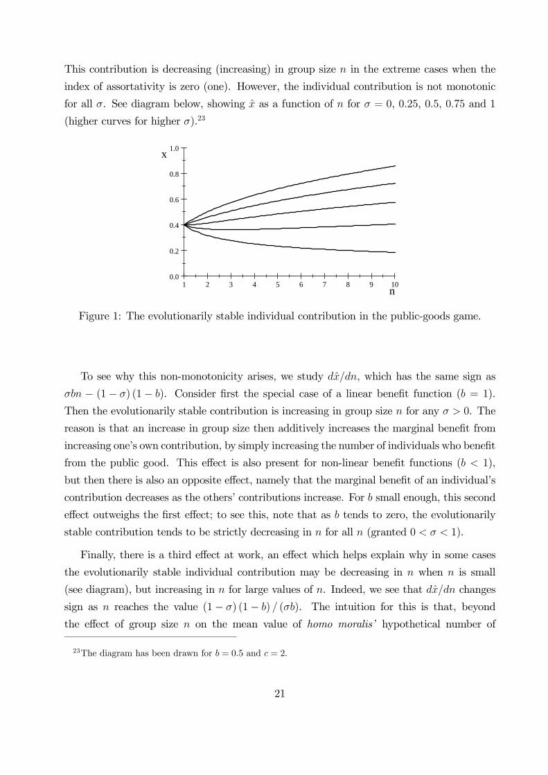
This contribution is decreasing (increasing) in group size in the extreme cases when the
index of assortativity is zero (one). However, the individual contribution is not monotonic
for all . See diagram below, showing as a function of for = 0, 025, 05, 075 and 1
(higher curves for higher ).23
1 2 3 4 5 6 7 8 9 100.0
0.2
0.4
0.6
0.8
1.0
n
x
Figure 1: The evolutionarily stable individual contribution in the public-goods game.
To see why this non-monotonicity arises, we study , which has the same sign as
− (1− ) (1− ). Consider first the special case of a linear benefit function ( = 1).
Then the evolutionarily stable contribution is increasing in group size for any 0. The
reason is that an increase in group size then additively increases the marginal benefit from
increasing one’s own contribution, by simply increasing the number of individuals who benefit
from the public good. This effect is also present for non-linear benefit functions ( 1),
but then there is also an opposite effect, namely that the marginal benefit of an individual’s
contribution decreases as the others’ contributions increase. For small enough, this second
effect outweighs the first effect; to see this, note that as tends to zero, the evolutionarily
stable contribution tends to be strictly decreasing in for all (granted 0 1).
Finally, there is a third effect at work, an effect which helps explain why in some cases
the evolutionarily stable individual contribution may be decreasing in when is small
(see diagram), but increasing in for large values of . Indeed, we see that changes
sign as reaches the value (1− ) (1− ) (). The intuition for this is that, beyond
the effect of group size on the mean value of homo moralis’ hypothetical number of
23The diagram has been drawn for = 05 and = 2.
21
others who contribute likewise, (− 1), there is an effect on the variance of this number,(− 1) (1− ), and hence on the risk that others might not contribute much. Indeed, a
vanishingly rare mutant faces considerable uncertainty as to the contributions his opponents
will make, when is small. For = 2, the uncertainty is hefty; a mutant’s opponent either
makes the same contribution or the resident contribution. As increases, the mutant’s
uncertainty becomes less hefty, since then the variance of the share of other contributors
tends to zero. For small, the riskiness may strong enough to reduce homo moralis’ incentive
to contribute more when when the group is larger.
Remark 1 The public goods interaction described here is symmetric. However, as noted
before, our general model also applies to asymmetric interactions as long as these are ex
ante symmetric, i.e. such that each individual at the outset is just as likely to be cast in
either player role (as, for instance, in a laboratory experiment). To illustrate, suppose that
only some individuals are free to give a contribution. More precisely, let ⊂ 1 denote the random set of active players. Suppose further that ex ante, each individual faces
the same probability ∈ (0 1) to get an active player role, that is, to be in the set . Aplayer’s strategy, is then a contribution to make if called upon to be active (without being
told who else is active). Let denote player ’s strategy so defined. We may then write the
ex ante payoff function of any player in the symmetric form
(x−) = ·Eh³X
∈
´| ∈
i− · ()+ (1− ) ·E
h³X
∈
´| ∈
i
where the expectation is taken with respect to the random draw of the subset .
6.2 Team work
Suppose instead that the jointly produced good in the previous example is a private good,
split evenly between the members of the group or team. The same analysis applies, with the
only difference that the individual benefit be divided by . One then obtains the following
necessary and sufficient condition for the evolutionarily stable individual contribution:
[1 + (− 1)] ·0 () = · 0 ()
Comparing this with the public goods case (equation (24)), we note that the evolution-
arily stable individual contribution now is smaller, that it is still increasing in the index of
assortativity, and that it is now necessarily decreasing in group size.
22
6.3 Contests
Many real interactions involve competing for a prize. Examples include competition between
job seekers for a vacancy, between firms for a contract, between employees for promotion, etc.
Such interactions may be modeled as a contest in which each participant makes a nonnegative
effort at some personal cost, and where each participant’s effort probabilistically translates
to a “result,” and the participant with the “best” result wins the prize. More specifically, let
≥ 0 be participant 0s effort, x− the vector of efforts of the others, and let = + be
participant ’s result (as valued by the “umpire”). With absolutely continuously distributed
random terms, ties occur with probability zero. For quadratic costs of effort, the material
payoff to participant is:
(x−) = · Pr [ ∀ 6= ]− 122 (25)
where 0 is the value of the prize in question. This defines a continuously and (infinitely)
differentiable function on = R+. For Gumbel distributed random terms, the winning
probability for each participant satisfies24
Pr [ ∀ 6= ] =P
=1 ∀ ∈
From this it is easily verified that a necessary condition (22) for an effort level 0 to be
evolutionarily stable boils down to
=1−
·µ1− 1
¶· (26)
The evolutionarily stable individual effort is proportional to the value of the price, linearly
decreasing (towards zero) in the index of assortativity, , and decreasing in (for all ≥ 2).Aggregate effort, however, is increasing in .
6.4 Helping others
People often help others, also when no reward or reciprocation is expected. To model such
behaviors, consider a group of ex ante identical individuals, and suppose that with some
exogenous probability ∈ (0 1) exactly one individual loses one unit of wealth, with equalprobability for all individuals when this happens. The − 1 others observe this event, and
24This is a standard result in random utility theory, see, e.g., Anderson et al. (1992).
23
each of them may then help the unfortunate individual by transferring some personal wealth.
These decisions are voluntary and simultaneous. For any individual level of wealth ≥ 0,let () be the individual’s indirect utility from consumption, where meets the usual
Inada conditions.
We model this as a game where initial wealth is normalized to unity:
(x−) = (1− ) · (1) + ·"µ1− 1
¶ (1− ) +
1
ÃX 6=
!#Here ≥ 0 is ’s voluntary transfer in case another individual is hit by the wealth loss.
Applying equation (24), for an individual transfer ∈ (0 1) to be evolutionarily stable, itmust satisfy
0 (1− ) = · 0 [(− 1) ] (27)
This equation uniquely determines ∈ (0 1), since the left-hand side is continuously andstrictly increasing in , from 0 (1) towards plus infinity, and the right-hand side is contin-
uously and strictly decreasing in , from plus infinity to 0 (− 1). It follows immediatelyfrom (27) that this transfer is an increasing function of the index of assortativity and a
decreasing function of group size . Both effects are intuitively expected; higher assortativ-
ity makes helpfulness more worthwhile and more individuals watching the wealth-loss makes
free-riding among them the more severe. In the special case when indirect utility is a power
function, () ≡ for some ∈ (0 1), one obtains
=1(1−)
− 1 + 1(1−)
While no transfers are given under uniform random matching ( = 0), post-transfer wealth
levels are equalized when = 1, so full insurance then holds, while partial insurance obtains
for intermediate values of . Furthermore, it is easy to verify that the aggregate transfer,
, is increasing in and converges to 1(1−) as →∞.
7 Literature
When introduced by Maynard Smith and Price (1973) the concept of evolutionary stability
was defined as a property ofmixed strategies in finite and symmetric two-player games played
under uniform random matching in an infinite population, where uniform random matching
means that the probability for an opponent’s strategy does not depend on one’s own strat-
egy. Broom, Cannings and Vickers (1997) generalized Maynard Smith’s and Price’s original
24
definition to finite and symmetric -player games, for ≥ 2 arbitrary, while maintainingthe assumption of uniform random matching in an infinite population.25 They noted the
combinatorial complexity entailed by this generalization, and reported some new phenom-
ena that can arise when interactions involve more than two parties. Evolutionary stability
and asymptotic stability in the replicator dynamic, in the same setting, was further analyzed
by Bukowski and Miekisz (2004). Schaffer (1988) extended the definition of Maynard Smith
and Price to the case of uniform random matching in finite populations, and also consid-
ered interactions involving all individuals in the population (“playing the field”). Grafen
(1979) and Hines and Maynard Smith (1979) generalized the definition of Maynard Smith
and Price from uniform random matching to the kind of assortative matching that arises
when strategies are genetically inherited and games are played among kin.
Our model generalizes most of the above work within a unified framework. To see this,
note first how our definition of evolutionarily stability relates to Maynard Smith’s and Price’s
(1973) original definition of an evolutionarily stable (mixed) strategy in a symmetric and
finite two-player game under uniform randommatching. Suppose thus that is the unit sim-
plex of mixed strategies in such a game and let Θ = , that is, let a type be a mixed strategy
(as if individuals were “programmed” to strategies). For any population state = ( ) ∈2 × (0 1), the set () of possible material-payoff pairs is then a singleton. Its uniqueelement ∈ () has components 1 = (1− ) ( )+ ( ) = [ (1− ) + ] and
2 = (1− ) ( ) + ( ) = [ (1− )+ ]. In other words, 1 (resp. 2) is the
“post-entry” expected material payoff to strategy (resp. ). By Definition 1, is evolu-
tionarily stable against if ( ) 0 for all 0 sufficiently small, which is equivalent
with being evolutionarily stable in the sense of Maynard Smith and Price (1973). Suppose
a strategy is unstable in the sense of Definition 1. Since is here continuous, there then
exists a strategy 6= such that ( ) 0 for all 0 sufficiently small, that is, such
that this mutant’s post-entry expected material payoff exceeds that of the resident strategy
whenever the mutant appears in sufficiently small population shares. Second, note that
the functions and (see (12) and (13)) are generalizations, from uniform to assortative
matching, of the functions used by Broom, Cannings and Vickers (1997) in their definition
of an evolutionarily stable strategy in symmetric and finite -player games (here and
may be mixed strategies in a finite game).
25Precursors to their work are Haigh and Cannings (1989), Cannings and Whittaker (1995) and Broom,
Cannings and Vickers (1996).
25
In a pioneering study, Güth and Yaari (1992) defined evolutionary stability for para-
metrized utility functions, assuming uniform random matching and complete information.26
This approach is often referred to as “indirect evolution.” The literature on preference evo-
lution now falls into four broad classes, depending on whether the focus is on interactions
where information is complete27 or incomplete28, and whether non-uniform randommatching
is considered.29 Few models deal with interactions involving more than two individuals. Like
here, the articles in this category focus exclusively on interactions that are symmetric in ma-
terial payoffs, the payoffs that drive evolution. Unlike us, they restrict attention to uniform
random matching. Koçkesen, Ok, and Sethi (2000a,b) show that under complete informa-
tion about opponents’ preferences, players with a specific kind of interdependent preferences
fare better materially than players who seek to maximize their material payoff. Sethi and
Somanathan (2001) go one step further and characterize sufficient conditions for a popula-
tion of individuals with the same degree of reciprocity to withstand the invasion of selfish
individuals, again in a complete information framework. By contrast, Ok and Vega-Redondo
(2001) analyze the case of incomplete information. They identify sufficient conditions for a
population of selfish individuals to withstand the invasion by non-selfish individuals, and for
selfish individuals to be able to invade a population of identical non-selfish individuals.
8 Conclusion
To understand human societies it is necessary to understand humanmotivation. In this paper
we build on a large literature in biology and in economics, initiated by Maynard Smith and
Price (1973), to propose a theoretical framework within which one may study the evolution
of human motivational types by way of natural selection. The framework is based upon a
26See also Frank (1987).
27See Robson (1990), Güth and Yaari (1992), Ockenfels (1993), Huck and Oechssler (1996), Ellingsen
(1997), Bester and Güth (1998), Fershtman and Judd (1987), Fershtman and Weiss (1998), Koçkesen, Ok
and Sethi (2000a,b), Bolle (2000), Possajennikov (2000), Sethi and Somanathan (2001), Heifetz, Shannon
and Spiegel (2007a,b), Akçay et al. (2009), Alger (2010), and Alger and Weibull (2010, 2012).
28See Ok and Vega-Redondo (2001), Dekel, Ely and Yilankaya (2007), and Alger and Weibull (2013).
29In the literature cited in the preceding two footnotes, only Alger (2010), Alger and Weibull (2010, 2012,
2013) allow for non-uniform random matching. Bergstrom (1995, 2003) also allows for such assortative
matching, but he restricts attention to strategy rather than preference evolution.
26
general definition of an evolutionarily stable type, where an individual’s type guides his or her
behavior in interactions in groups of any size. The framework may be applied to interactions
where others’ preferences are known or unknown, and it allows for assortativity in the process
by which individuals are matched together to interact. Since our analysis focuses on whether
a homogenous population may withstand a small-scale invasion of individuals of a different
type, a key factor is the probability with which mutants are matched with other mutants
when these are vanishingly rare. In two-player interactions, such assortativity is simply the
probability that the individual with whom a mutant interacts also is a mutant (the index
of assortativity; Bergstrom, 2003). We generalize this notion to -player interactions by
defining the assortativity profile of an -party matching process, for which the assortativity
profile is a vector that provides the probabilities that none, some, or all the individuals
with whom a mutant interacts also are mutants, in the limit as the share of mutants in the
population tends to zero. There is some assortativity as soon as the probability that at least
one of the individuals with whom a mutant interacts also is a mutant is positive.
We apply the framework to preference evolution when an individual’s preferences are
his or her private information. The set of potential preferences is taken to be the set of
all continuous and aggregative preferences over strategy profiles. Our analysis shows that a
particular preference comes out as a clear winner in the evolutionary race. This preference
belongs to the class of homo moralis preferences, according to which an individual maximizes
a weighted sum of the material payoff that she would obtain if none, some, or all the indi-
viduals with whom she interacts would do as she does; the weights represent the individual’s
morality profile. More precisely, we find that (a) homo moralis preferences with a morality
profile that reflects the assortativity in the matching process are evolutionarily stable, and
(b) under quite weak assumptions, any preferences that lead to different behaviors from that
of this homo moralis are evolutionarily unstable. Furthermore, equilibrium behavior in a
homogeneous population consisting of homo moralis with this type of morality is the same
as under strategy evolution.
Interestingly, then, our analysis shows that group size has no effect on what class of
preferences is favored by evolution when preferences are the interacting individuals’ private
information; homo moralis preferences with a morality profile equal to the assortativity
profile stand out as the clear winner in the evolutionary race, independent of group size and
of the (material) game played. By contrast, as shown in the examples, group size does affect
equilibrium behavior, in groups consisting of identical homo moralis. Assuming conditional
independence in the matching process, we found that, for any positive index of assortativity
27
, the evolutionarily stable variety of homo moralis contributes more than homo oeconomicus
in public-goods games and also when in team work. By contrast, she exerts less effort in
contests and supplies less output in Cournot markets. She is also helpful to others who have
been exposed to an exogenous hazard. Moreover, these effects do not generally vanish as
group size increases. This is because homo moralis behaves as if she, roughly speaking
thought “what would happen if the share of the other group members would do like me?”
when contemplating her strategy choice.30
Although quite general, our model relies on a number of simplifying assumptions. Relax-
ation of these is a task that has to be left for future research. Moreover, we only apply our
general definition of evolutionary stability to two cases, strategy evolution and preference
evolution when preferences are private information. Applications to complete or partially
incomplete information are called for, in particular in settings where the random matching is
not exogenous, as here, but at least partly endogenous. This is a major analytical challenge,
however, opening the door to signalling and mimicry, a very rich, important and exciting
research area. Yet another challenge would be to investigate evolutionary neutrality, setwise
evolutionary stability and/or evolutionary stability properties of heterogenous population
states.
For the past twenty years or so economists have proposed varieties of pro-social or other-
regarding preference in order to explain certain observed behaviors, mostly in laboratory
experiments but sometimes in the field, that are at odds with maximization of one’s own
material payoff. Our research has so far delivered two results of relevance for behavioral
economics. First, the result that natural selection selects preferences with a distinct Kantian
flavor; it is as if individuals in their strategy choice attach some importance to “what would
happen if others did what I do?” Homo oeconomicus is an extreme case; to place no impor-
tance at all to this Kantian morality aspect. Second, we have the result that the importance
that individuals attach to this Kantian morality aspect depends on the assortativity in the
matching process, and is independent of the interaction in question. Since historically, as-
sortativity arguably has varied between populations and over time (depending on geography,
technology and social structure), this second result suggests that one should expect the im-
portance of morality to differ accordingly. Likewise, our results suggest that if in a population
30We here invoke the law of large numbers, which holds under conditional independence, but arguing
heuristically, as if the expected value of the average of a function has the same qualitative features as the
function evaluated at the average point.
28
individuals interact in several different games, and assortativity differs between the games
(e.g., sharing with relatives, and engaging in market interactions with strangers), then one
should expect different levels of morality in the different games. We hope that our theoretical
results, combined with empirical and experimental work, will enhance the understanding of
human behavior and motivation.
9 Appendix: A class of matching processes
Let , and be integers greater than one, and imagine a finite population consisting of
individuals. The population is divided into “islands,” each island consisting of
individuals, and is some multiple of . Initially all individuals are of type . Suddenly
a mutation to another type occurs in one of the islands, and only there. Each individual
on that island has probability of mutating, and individual mutations are statistically
independent. Hence, the random number of mutants is binomially distributed ∼ ( ). We note that in this mutation process the random number is also the total
number of mutants in the population at large, so the population share of mutants is
a random variable with expectation = E [ ] = . A group of size is now formed
to play a game Γ = h i (as described in Section 2) as follows, and this is an eventthat is statistically independent of the above-mentioned mutation. First, one of the islands
is selected, with equal probability for each island. Secondly, individuals from the selected
island are recruited to form the group, drawn as a random sample without replacement from
amongst the islanders and with equal probability for each islander to be sampled.
Consider an individual who has been recruited to the group. Let ∈ denote theindividual’s type. If = , it is necessary that 0 and that the individual is from the
island where the mutation occurred, so the random number of other mutants in her group
is binomially distributed, (− 1 ). With denoting the total number of mutants in
her group, we have, for = 1 2 :
Pr [ = | = ] =
Ã− 1− 1
!−1 (1− )
− (28)
If instead = , then = 0 is possible and she may well be from another island than
where the mutation occurred. We thus have
Pr [ = | = ] ≤
·Ã
− 1
! (1− )
−−1
29
for all 0. Moreover, for any two group members and :
Pr [ = | = ] = and Pr [ = | = ] ≤
Keeping , and constant, we may write Pr [| ] for Pr [ = | = ] andPr [| ]for Pr [ = | = ], and these conditional probabilities are continuous functions of =
. In addition, we have 1− ≤ Pr [| ] ≤ 1 and Pr [| ] = 1− . Letting →∞,we obtain → 0 and Pr [| ] → 1. Hence, lim→0 () = , so in this example the index
of assortativity is = .
References
Acemoglu, D. and M.K. Jensen (2013) “Aggregate comparative statics,” Games and
Economic Behavior, 81, 27 - 49.
Akçay, Erol, Jeremy Van Cleve, Marcus W. Feldman, and Joan Roughgarden (2009) “A
Theory for the Evolution of Other-Regard Integrating Proximate and Ultimate Perspectives,”
Proceedings of the National Academy of Sciences, 106, 19061—19066.
Alger, I. (2010): “Public Goods Games, Altruism, and Evolution,” Journal of Public
Economic Theory, 12, 789-813.
Alger, I. and J. Weibull (2010): “Kinship, Incentives and Evolution,”American Economic
Review, 100, 1725-1758.
Alger, I. and J. Weibull (2012): “A Generalization of Hamilton’s Rule–Love Others How
Much?” Journal of Theoretical Biology, 299, 42-54.
Alger, I. and J. Weibull (2013): “Homo Moralis–Preference Evolution under Incomplete
Information and Assortative Matching,” Econometrica, 81:2269-2302.
Aliprantis, C.D. and K.C. Border (2006): Infinite Dimensional Analysis, 3rd ed. New
York: Springer.
Anderson, S.P., A. de Palma, and J.-F. Thisse (1992): Discrete Choice Theory of Product
Differentiation. VCambridge (USA): MIT Press.
Andreoni, J. (1990): “Impure Altruism and Donations to Public Goods: A Theory of
Warm-Glow Giving,” Economic Journal, 100, 464-477.
Becker, G. (1976): “Altruism, Egoism, and Genetic Fitness: Economics and Sociobiol-
ogy,” Journal of Economic Literature, 14, 817—826.
30
Bénabou, R. and J. Tirole (2006): “Incentives and Prosocial Behavior,” American Eco-
nomic Review, 96, 1652-1678.
Bergstrom, T. (1995): “On the Evolution of Altruistic Ethical Rules for Siblings,” Amer-
ican Economic Review, 85, 58-81.
Bergstrom, T. (2003): “The Algebra of Assortative Encounters and the Evolution of
Cooperation,” International Game Theory Review, 5, 211-228.
Bergstrom, T. (2009): “Ethics, Evolution, and Games among Neighbors,” Working Pa-
per, UCSB.
Bergstrom, T. (2013): “Measures of Assortativity,” Biological Theory, 8, 133-141.
Bester, H. and W. Güth (1998): “Is Altruism Evolutionarily Stable?” Journal of Eco-
nomic Behavior and Organization, 34, 193—209.
Bolle, F. (2000): “Is Altruism Evolutionarily Stable? And Envy and Malevolence? Re-
marks on Bester and Güth” Journal of Economic Behavior and Organization, 42, 131-133.
Bomze, I., and B. Pötscher (1989): Game Theoretical Foundations of Evolutionary Sta-
bility. New York: Springer.
Bramoullé, Y., and B. Rogers (2009): “Diversity and Popularity in Social Networks,”
Discussion Papers 1475, Northwestern University, Center for Mathematical Studies in Eco-
nomics and Management Science.
Brekke, K.A., S. Kverndokk, and K. Nyborg (2003): “An economic model of moral
motivation,” Journal of Public Economics, 87, 1967-1983.
Broom, M., C. Cannings and G.T. Vickers (1996): “Choosing a Nest Site: Contests and
Catalysts”, Amer. Nat. 147, 1108-1114.
Broom, M., C. Cannings and G.T. Vickers (1997): “Multi-Player Matrix Games”, Bul-
letin of Mathematical Biology 59, 931-952.
Bukowski, M., and J. Miekisz (2004): “Evolutionary and asymptotic stability in sym-
metric multi-player games”, International Journal of Game Theory 33, 41-54.
Cannings, C., and J.C. Whittaker (1995): “The Finite Horizon War of Attrition", Games
and Economic Behavior 11, 193-236.
Corchón, L. (1996): Theories of Imperfectly Competitive Markets. Berlin: Springer Ver-
lag.
31

Currarini, S., M.O. Jackson, and P. Pin (2009): “An Economic Model of Friendship:
Homophily, Minorities and Segregation,” Econometrica, 77, 1003—1045.
Currarini, S., M.O. Jackson, and P. Pin (2010): “Identifying the Roles of Race-Based
Choice and Chance in High School Friendship Network Formation,” Proceedings of the Na-
tional Academy of Sciences, 107, 4857—4861.
Day, T., and P.D. Taylor (1998): “Unifying Genetic and Game Theoretic Models of Kin
Selection for Continuous types,” Journal of Theoretical Biology, 194, 391-407.
Dekel, E., J.C. Ely, and O. Yilankaya (2007): “Evolution of Preferences,” Review of
Economic Studies, 74, 685-704.
Dubey, P., A. Mas-Colell, and M. Shubik (1980): “Efficiency Properties of Strategic
Market Games”, Journal of Economic Theory 22, 339-362.
Duffie, D. and Y. Sun (2012): “The Exact Law of Large Numbers for Independent Ran-
dom Matching", Journal of Economic Theory 147, 1105-1139.
Ellingsen, T. (1997): “The Evolution of Bargaining Behavior,” Quarterly Journal of
Economics, 112, 581-602.
Fehr, E., and K. Schmidt (1999): “A theory of Fairness, Competition, and Cooperation,”
Quarterly Journal of Economics, 114, 817-868.
Fershtman, C. and K. Judd (1987): “Equilibrium Incentives in Oligopoly,” American
Economic Review, 77, 927—940.
Fershtman, C., and Y. Weiss (1998): “Social Rewards, Externalities and Stable Prefer-
ences,” Journal of Public Economics, 70, 53-73.
Frank, R.H. (1987): “If Homo Economicus Could Choose His Own Utility Function,
Would He Want One with a Conscience?” American Economic Review, 77, 593-604.
Grafen, A. (1979): “The Hawk-Dove Game Played between Relatives,” Animal Behavior,
27, 905—907.
Grafen, A. (2006): “Optimization of Inclusive Fitness,” Journal of Theoretical Biology,
238, 541—563.
Güth, W., and M. Yaari (1992): “An Evolutionary Approach to Explain Reciprocal Be-
havior in a Simple Strategic Game,” in U.Witt. Explaining Process and Change — Approaches
to Evolutionary Economics. Ann Arbor: University of Michigan Press.
32
Haigh, J., and C. Cannings (1989): “The n-Person War of Attrition”, Acta Applic. Math.
14, 59-74.
Hamilton, W.D. (1964a): “The Genetical Evolution of Social Behaviour. I.” Journal of
Theoretical Biology, 7:1-16.
Hamilton, W.D. (1964b): “The Genetical Evolution of Social Behaviour. II.” Journal of
Theoretical Biology, 7:17-52.
Heifetz, A., C. Shannon, and Y. Spiegel (2007a): “The Dynamic Evolution of Prefer-
ences,” Economic Theory, 32, 251-286.
Heifetz, A., C. Shannon, and Y. Spiegel (2007b): “What to Maximize if You Must,”
Journal of Economic Theory, 133, 31-57.
Hines, W.G.S., and J. Maynard Smith (1979): “Games between Relatives,” Journal of
Theoretical Biology, 79, 19-30.
Huck, S., and J. Oechssler (1999): “The Indirect Evolutionary Approach to Explaining
Fair Allocations,” Games and Economic Behavior, 28, 13—24.
Jackson, M.O., and A. Watts (2010): “Social Games: Matching and the Play of Finitely
Repeated Games,” Games and Economic Behavior, 70, 170-191.
Koçkesen, L., E.A. Ok, and R. Sethi (2000a): “The Strategic Advantage of Negatively
Interdependent Preferences,” Journal of Economic Theory, 92, 274-299.
Koçkesen, L., E.A. Ok, and R. Sethi (2000b): “Evolution of Interdependent Preferences
in Aggregative Games,” Games and Economic Behavior 31, 303-310.
Levine, D. (1998): “Modelling Altruism and Spite in Experiments,” Review of Economic
Dynamics, 1, 593-622.
Luenberger, D.G. 1969. Optimization by Vector Space Methods. New York: John Wiley
& Sons.
Maynard Smith, J., and G.R. Price (1973): “The Logic of Animal Conflict,” Nature,
246:15-18.
McPherson, M., L. Smith-Lovin, and J.M. Cook (2001): “Birds of a Feather: Homophily
in Social Networks,” Annual Review of Sociology, 27, 415-444.
Munkres, James (1975): Topology, a First Course. London: Prentice Hall.
Ockenfels, P. (1993): “Cooperation in Prisoners’ Dilemma–An Evolutionary Approach”,
33
European Journal of Political Economy, 9, 567-579.
Ok, E.A., and F. Vega-Redondo (2001): “On the Evolution of Individualistic Preferences:
An Incomplete Information Scenario,” Journal of Economic Theory, 97, 231-254.
Possajennikov, A. (2000): “On the Evolutionary Stability of Altruistic and Spiteful Pref-
erences” Journal of Economic Behavior and Organization, 42, 125-129.
Robson, A.J. (1990): “Efficiency in Evolutionary Games: Darwin, Nash and the Secret
Handshake,” Journal of Theoretical Biology, 144, 379-396.
Robson, A.J., and B. Szentes (2014): “A Biological Theory of Social Discounting,” forth-
coming, American Economic Review.
Roemer, J.E. (2010): “Kantian equilibrium,” Scandinavian Journal of Economics, 112,
1-24.
Ruef, M., H.E. Aldrich, and N.M. Carter (2003): “The Structure of Founding Teams:
Homophily, Strong Ties, and Isolation among U.S. Entrepreneurs,” American Sociological
Review, 68, 195-222.
Sandholm, W. (2001): “Preference Evolution, Two-Speed Dynamics, and Rapid Social
Change,” Review of Economic Dynamics, 4, 637-679.
Schaffer, M.E. (1988): “Evolutionarily Stable Strategies for Finite Populations and Vari-
able Contest Size,” Journal of Theoretical Biology, 132, 467-478.
Schelling, T. (1960): The Strategy of Conflict. Cambridge: Harvard University Press.
Sethi, R., and E. Somanathan (2001): “Preference Evolution and Reciprocity” Journal
of Economic Theory, 97, 273-297.
Weibull, J.W. (1995): Evolutionary Game Theory. Cambridge: MIT Press.
Weibull, J.W. (2004): “Testing Game Theory”, in S. Huck (ed.): Advances in Under-
standing Strategic Behaviour: Game Theory, Experiments, and Bounded Rationality - Essays
in Honor of Werner Güth. Palgrave MacMillan.
34