evolution of regression ols to gps to mars
TRANSCRIPT
1Salford Systems ©2013
Evolution of Regression:From Classical Least Squares to
Regularized Regression to Machine Learning Ensembles
Covering MARS®, Generalized PathSeeker®,
TreeNet® Gradient Boosting and Random Forests®
A Brief Overview the 4 Part Webinarat www.salford-systems.com
May 2013Dan Steinberg
Mikhail Golovnya
Salford Systems

Salford Systems ©2013 2
Full Webinar Outline
• Regression Problem – quick overview• Classical Least Squares – the starting point• RIDGE/LASSO/GPS – regularized regression• MARS – adaptive non-linear regression splines
• CART Regression tree– quick overview• Random Forest decision tree ensembles• TreeNet Stochastic Gradient Boosted Trees• Hybrid TreeNet/GPS (trees and regularized regression)
Webinar Part 1
Webinar Part 2

Salford Systems ©2013 3
Regression• Regression analysis at least 200 years old
o most used predictive modeling technique (including logistic regression)
• American Statistical Association reports 18,900 memberso Bureau of Labor Statistics reports more than 22,000 statisticians in 2008
• Many other professionals involved in the sophisticated analysis of data not included in these countso Statistical specialists in marketing, economics, psychology, bioinformaticso Machine Learning specialists and ‘Data Scientists’o Data Base professionals involved in data analysiso Web analytics, social media analytics, text analytics
• Few of these other researchers will call themselves statisticianso but may make extensive use of variations of regression
• One reason for popularity of regression: effective

Salford Systems ©2013 4
Regression Challenges• Preparation of data – errors, missing values, etc.
o Largest part of typical data analysis (modelers often report 80% time)
o Missing values a huge headache (listwise deletion of rows)
• Determining which predictors to include in modelo Text book examples typically have 10 predictors availableo Hundreds, thousands, even tens and hundreds of thousands available
• Transformation or coding of predictorso Conventional approaches: logarithm, power, inverse, etc..o Required to obtain a good model
• High correlation among predictorso With increasing numbers of predictors this complication
becomes more serious

Salford Systems ©2013 5
More Regression Challenges
• Obtaining “sensible” results (correct signs, no wild outcomes)
• Detecting and modeling important interactionso Typically never done because too difficult
• “Wide” data has more columns than rows• Lack of external knowledge or theory to guide
modeling as more topics are modeled

Salford Systems ©2013 6
Boston Housing Data Set• Concerns the housing values in Boston area• Harrison, D. and D. Rubinfeld. Hedonic Prices and
the Demand For Clean Air. o Journal of Environmental Economics and Management, v5, 81-102 , 1978
• Combined information from 10 separate governmental and educational sources to produce data set
•506 census tracts in City of Boston for the year 1970o Goal: study relationship between quality of life variables and property valueso MV median value of owner-occupied homes in tract ($1,000’s)o CRIM per capita crime rateso NOX concentration nitric oxides (p.p. 10 million) proxy for air pollution generallyo AGE percent built before 1940o DIS weighted distance to centers of employmento RM average number of rooms per houseo LSTAT % lower status of population (without some high school and male laborers)o RAD index of accessibility to radial highwayso CHAS borders Charles River (0/1)o INDUS percent of acreage non-retail businesso TAX property tax rate per $10,000o PT pupil teacher ratioo ZN proportion of neighborhood zoned for large lots (>25K sq ft)

Salford Systems ©2013 7
Ten Data Sources Organized
• US Census (1970)• FBI (1970)• MIT Boston Project• Metropolitan Area Planning Commission (1972)• Voigt, Ivers, and Associates (1965) (Land Use Survey)• US Census Tract Maps• Massachusetts Dept Of Education (1971-1972)• Massachusetts Tax Payer’s Foundation (1970)• Transportation and Air Shed Simulation Model, Ingram, et. al. Harvard
University Dept of City and Regional Planning (1974)• A. Schnare: An Empirical Analysis of the dimensions of neighborhood
quality. Ph.D. Thesis. Harvard. (1974)
• An excellent example of creative data blending• Also excellent example of careful model construction• Authors emphasize the quality (completeness of their data)

Salford Systems ©2013 8
Least Squares Regression• LS – ordinary least squares regression
o Discovered by Legendre (1805) and Gauss (1809) o Solve problems in astronomy using pen and papero Statistical foundation by Fisher in 1920so 1950s – use of electro-mechanical calculators
• The model is always of the form
• The response surface is a hyper-plane!• A – the intercept term• B1, B2, B3, … – parameter estimates
• A usually unique combination of values exists which minimizes the mean squared error of predictions on the learn sample
• Experimental approach to model building
Response = A + B1X1 + B2X2 + B3X3 + …
Salford Systems ©2013 9
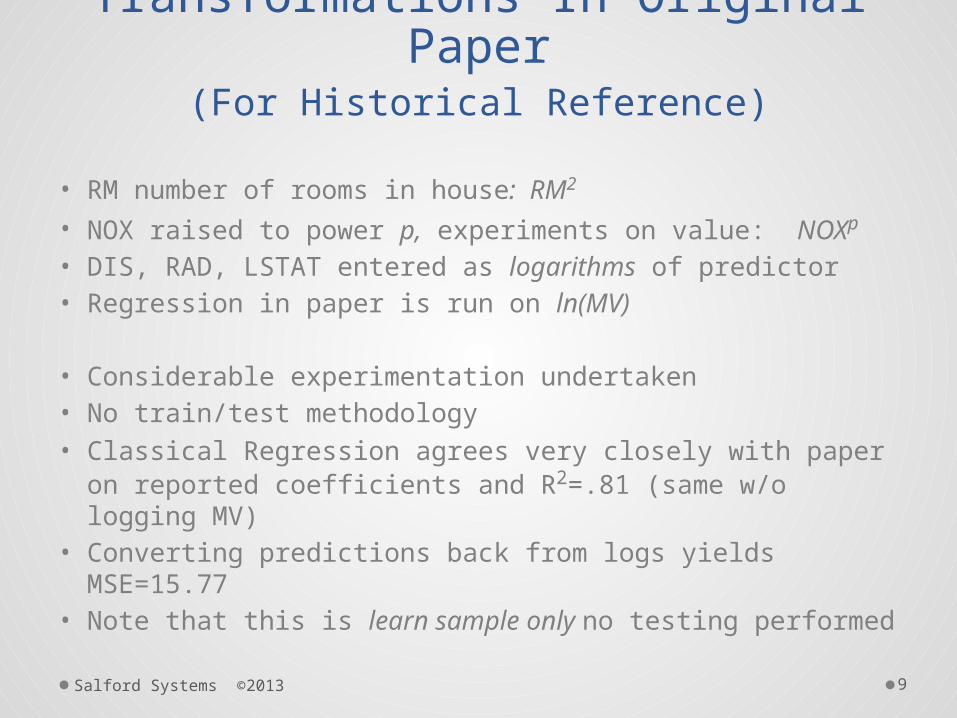
Transformations In Original Paper(For Historical Reference)
• RM number of rooms in house: RM2
• NOX raised to power p, experiments on value: NOXp
• DIS, RAD, LSTAT entered as logarithms of predictor• Regression in paper is run on ln(MV)
• Considerable experimentation undertaken• No train/test methodology• Classical Regression agrees very closely with paper on
reported coefficients and R2=.81 (same w/o logging MV)• Converting predictions back from logs yields
MSE=15.77• Note that this is learn sample only no testing performed
Salford Systems ©2013 10
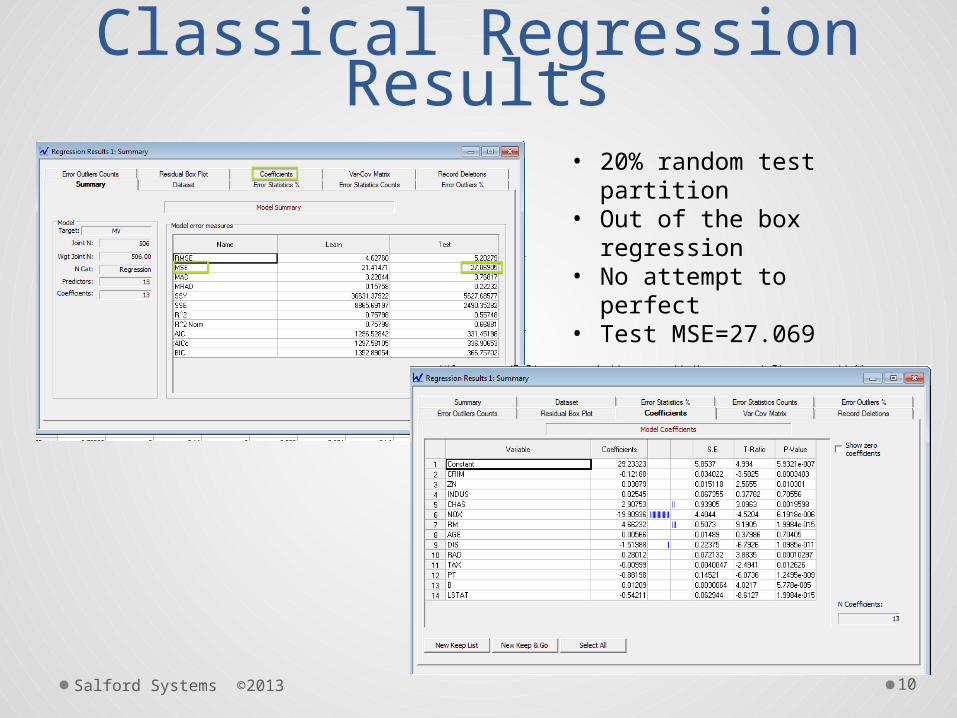
Classical Regression Results
• 20% random test partition
• Out of the box regression
• No attempt to perfect • Test MSE=27.069

Salford Systems ©2013 11
BATTERY PARTITION: Rerun 80/20 Learn test 100
times
Note partition sizes are constantAll three partitions change each cycleMean MSE=23.80
Salford Systems ©2013 12
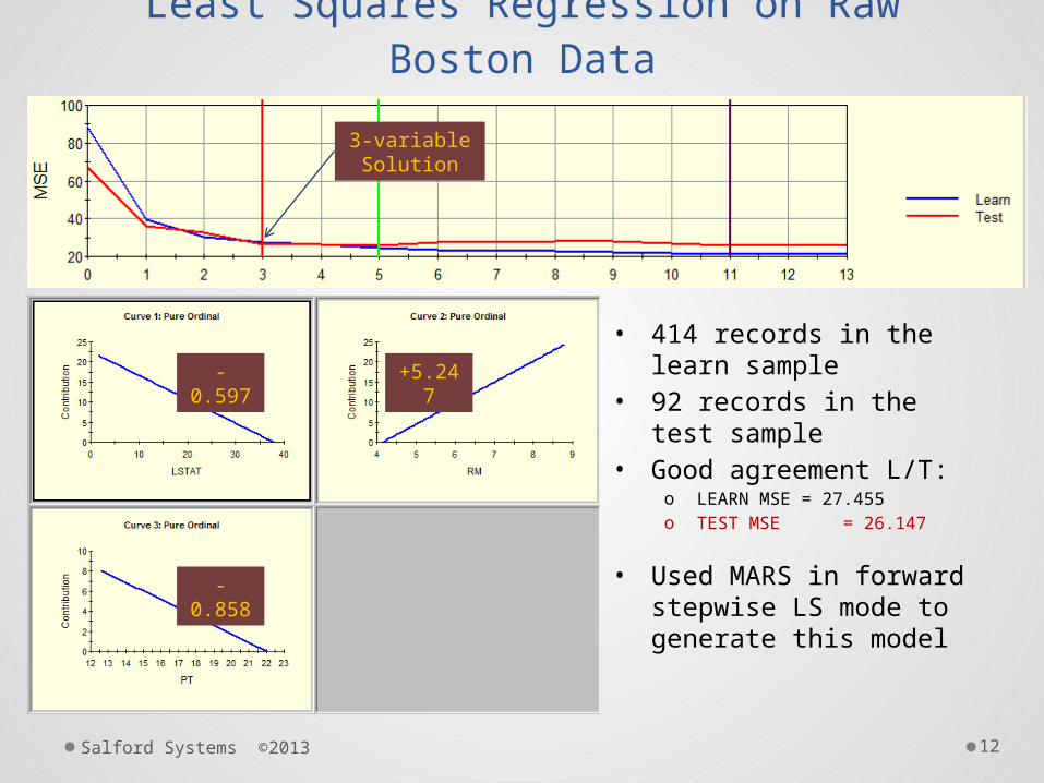
Least Squares Regression on Raw Boston Data
• 414 records in the learn sample
• 92 records in the test sample
• Good agreement L/T:o LEARN MSE = 27.455o TEST MSE = 26.147
• Used MARS in forward stepwise LS mode to generate this model
3-variable Solution
-0.597 +5.247
-0.858

Salford Systems ©2013 13
Motivation for Regularized Regression1960s and 1970s
• Unsatisfactory results based modeling physical processes o Coefficients changed dramatically with small changes in datao Some coefficients judged to be too largeo Appearance of coefficients with “wrong sign”o Severe with substantial correlations among predictors
(multicollinearity)
• Solution (1970) Hoerl and Kennard, “Ridge Regression”
• Earlier version just for stabilization of coefficients 1962o Initially poorly received by statistics profession

Salford Systems ©2013 14
Regression Formulas• X matrix of potential predictors (NxK)• Y column: the target or dependent variable (Nx1)
• Estimated b = (X’X)-1(X’y) standard formula• Ridge = b (X’X + rI)-1(X’y)• Simplest version: constant added to diagonal
elements of the X’X matrix• r=0 yields usual LS
• r=∞ yields degenerate model =0b• Need to find r that yields best generalization error• Observe that there is a potentially distinct
“solution” for every value of the penalty term r• Varying r traces a path of solutions

Salford Systems ©2013 15
Ridge Regression
• “Shrinkage” of regression coefficients towards zero• If zero correlation among all predictors then shrinkage
will be uniform over all coefficients (same percentage)• If predictors correlated then while the length of the
coefficient vector decreases some coefficients might increase (in absoluter value)
• Coefficients intentionally biased but yields both more satisfactory estimates and superior generalizationo Better performance (test MSE) on previously unseen data
• Coefficients much less variable even if biased• Coefficients will be typically be closer to the “truth”
Salford Systems ©2013 16
Ridge Regression Features
• Ridge frequently fixes the wrong sign problem• Suppose you have K predictors which happen to
be exact copies of each other• RIDGE will give each a coefficient equal to 1/K
times the coefficient that would be given to just one copy in a model
Salford Systems ©2013 17
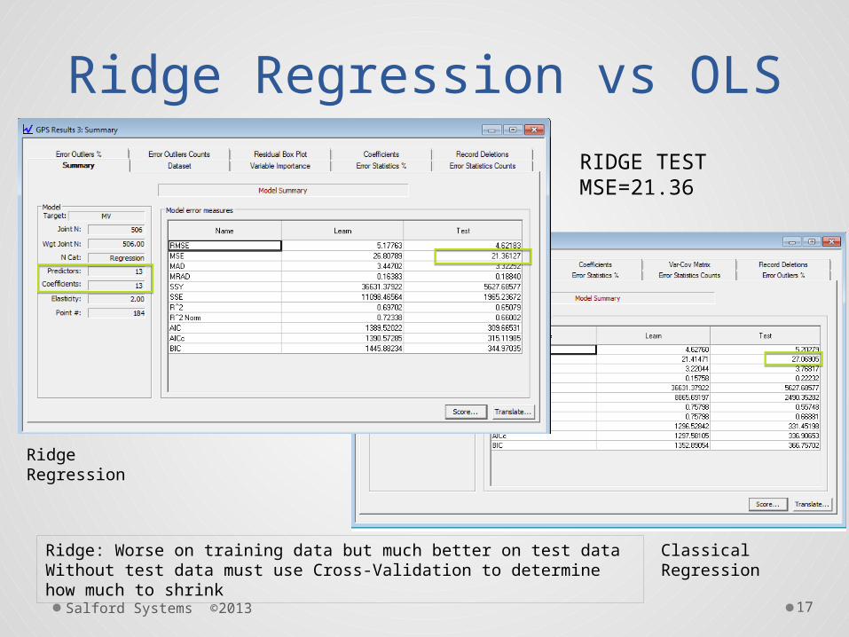
Ridge Regression vs OLS
Ridge Regression
Classical Regression
Ridge: Worse on training data but much better on test dataWithout test data must use Cross-Validation to determine how much to shrink
RIDGE TEST MSE=21.36

Salford Systems ©2013 18
Lasso Regularized Regression
• Tibshirani (1996) an alternative to RIDGE regression
• Least Absolute Shrinkage and Selection Operator
• Desire to gain the stability and lower variance of ridge regression while also performing variable selection
• Especially in the context of many possible predictors looking for a simple, stable, low predictive variance model
• Historical note: Lasso inspired by related work (1993) by Leo Breiman (of CART and RandomForests fame) ‘non-negative garotte’.
• Breiman’s simulation studies showed the potential for improved prediction via selection and shrinkage

Salford Systems ©2013 19
Regularized Regression -
Concepts
• Any regularized regression approach tries to balance model performance and model complexity
• λ – regularization parameter, to be estimatedo λ = ∞ Null model zero-coefficients (maximum possible penalty)o λ = 0 LS solution (no penalty)
Mean Squared Error Model Complexity
LS Regression
Minimize
Minimize
Regularized Regression
Ridge: Sum of squared
coefficients
Lasso: Sum of absolute
coefficients
Compact: Number of coefficients
λ

Salford Systems ©2013 20
Regularized Regression: Penalized Loss
Functions
• RIDGE penalty Sb2 squared b
• LASSO penalty |S b| absolute value b
• COMPACT penalty |S b|0 count of bs
• General penalty |S b| r 0<= <=2r
• RIDGE does no selection but Lasso and Compact select
• Power on b is called the “elasticity” ( 0, 1, 2)• Penalty to be estimated is a constant multiplying one of
the above functions of the b vector• Intermediate elasticities can be created: e.g. we
could have a 50/50 mix of RIDGE and LASSO yielding an elasticity of 1.5
Salford Systems ©2013 21
LASSO Features• With highly correlated predictors the LASSO will tend
to pick just one of them for model inclusion
• Dispersion of b greater than for RIDGE
• Unlike AIC and BIC model selection methods that penalize after the model is built these penalties
influence the bs
• A convenient trick for estimating models with regularization |S b| r is weighted average of any two of the major elasticities 0, 1, and 2. e.g.:
• wSb2 + (1-w) |S b| (the “elastic net”)

Salford Systems ©2013 22
Computational Challenge
• For a given regularization (e.g LASSO) find the optimal penalty on the b term
• Find the best regularization from the family |S b|r
• Potentially very many models to fit

Salford Systems ©2013 23
Computing Regularized Regressions -
1
• Earliest versions of regularized regressions required considerable computation as the penalty parameter is unknown and must be estimated
• Lasso was originally computed by starting with no penalty and gradually increasing the penaltyo So start with ALL vars in the modelo Gradually tighten the noose to squeeze predictors outo Infeasible for problems with thousands of possible predictors
• Need to solve a quadratic programming problem to optimize the Lasso solution for every penalty value
Salford Systems ©2013 24
Computing Regularized Regressions -
2
• Work by Friedman and others introduced very fast forward stepping approaches
• Start with maximum penalty (no predictors)• Progress forward with stopping rule
o Dealing with millions of predictors possible
• Coordinate gradient descent methods (next slides)• Will still want test sample or cross-validation for
optimization • Generalized PathSeeeker full range of regularization
from compact to Ridge (elasticies from 0 thru 2)• Glmnet in R partial range of regularization from Lasso
to Ridge (elasticities from 1 to 2)

Salford Systems ©2013 25
GPS Algorithm• Start with NO predictors in model• Seek the path b( ) n of solutions as function of
penalty strength
• Define pj( )=n dP/dbj marginal change in Penalty
• Define gj( ) = - n dR/dbj marginal change in Loss
• Define qj( )=n gj( )/n pj( ) n ratio (benefit/cost)
• Find max|qj( )| n to identify coefficient to update (j*)
• Update bj* in the direction of sign qj*
• - dR/dbj requires computing inner products of
current residual with available predictorso Easily parallelizable

Salford Systems ©2013 26
How to Forward Step• At any stage of model development choose between
• Add a new variable to Update an existing model variable coefficient
• Step sizes are small, initial coefficients for any model are very small and are updated in very small increments
• This explains why the Ridge elasticity can have solutions with less than all the variableso Technically ridge does not select variables, it only shrinkso In practice it can only add one variable per step

Salford Systems ©2013 27
Regularized Regression – Practical
Algorithm
• Start with the zero-coefficient solution• Look for best first step which moves one coefficient away from zero
o Reduces Learn Sample MSEo Increases Penalty as the model has become more complex
• Next step: Update one of the coefficients by a small amounto If the selected coefficient was zero, a new variable effectively enters into the modelo If the selected coefficient was not zero, the model is simply updated
CurrentModel
X1 0.0
X2 0.0
X3 0.2
X4 0.0
X5 0.4
X6 0.5
X7 0.0
X8 0.0
X1 0.0
X2 0.0
X3 0.2
X4 0.1
X5 0.4
X6 0.5
X7 0.0
X8 0.0
Introducing New Variable
NextModel
CurrentModel
X1 0.0
X2 0.0
X3 0.2
X4 0.0
X5 0.4
X6 0.5
X7 0.0
X8 0.0
X1 0.0
X2 0.0
X3 0.3
X4 0.1
X5 0.4
X6 0.5
X7 0.0
X8 0.0
Updating Existing Model
NextModel

Salford Systems ©2013 28
Path Building Process
• Elasticity Parameter – controls the variable selection strategy along the path (using the LEARN sample only), it can be between 0 and 2, inclusiveo Elasticity = 2 – fast approximation of Ridge Regression, introduces
variables as quickly as possible and then jointly varies the magnitude of coefficients – lowest degree of compression
o Elasticity = 1 – fast approximation of Lasso Regression, introduces variables sparingly letting the current active variables develop their coefficients – good degree of compression versus accuracy
o Elasticity = 0 – fast approximation of Best Subset Regression, introduces new variables only after the current active variables were fully developed – excellent degree of compression but may loose accuracy
ZeroCoefficient
Model
A Variableis Added
Sequence of
1-variablemodels A Variable
is Added
Sequence of
2-variablemodels
A Variableis Added
Sequence of
3-variablemodels
FinalOLS
Solution
Variable Selection Strategy
λ = ∞ λ = 0…

Salford Systems ©2013 29
Points Versus Steps
• Each path(elasticity) will have different number of steps• To facilitate model comparison among different paths,
the Point Selection Strategy extracts a fixed collection of models into the points grido This eliminates some of the original irregularity among individual paths and
facilitates model extraction and comparison
Path 2: Steps OLSSolution
Points
Path 1Path 2Path 3
ZeroSolution
Path 1: Steps
Path 3: Steps
Point Selection Strategy
1 2 3 4 5 6 7 8 9 10
1 2 3 4 5 6 7 8 9 10
1 2 3 4 5 6 7 8 9 10
Salford Systems ©2013 30
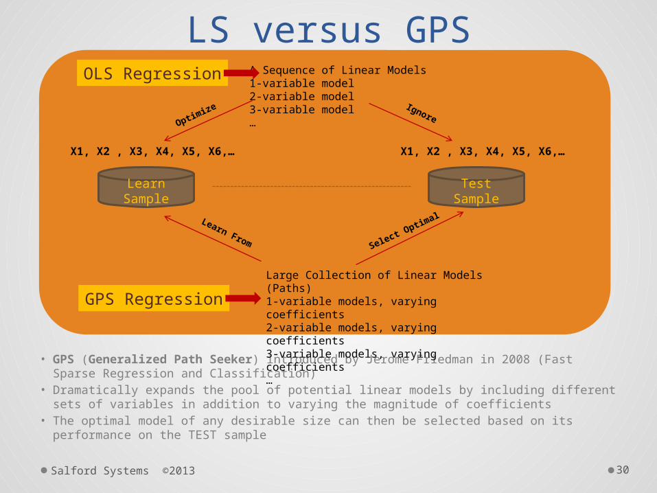
LS versus GPS
• GPS (Generalized Path Seeker) introduced by Jerome Friedman in 2008 (Fast Sparse Regression and Classification)
• Dramatically expands the pool of potential linear models by including different sets of variables in addition to varying the magnitude of coefficients
• The optimal model of any desirable size can then be selected based on its performance on the TEST sample
Learn Sample
OLS Regression
X1, X2 , X3, X4, X5, X6,…
Test Sample
X1, X2 , X3, X4, X5, X6,…
A Sequence of Linear Models1-variable model2-variable model3-variable model…Optim
ize Ignore
GPS Regression
Large Collection of Linear Models (Paths)1-variable models, varying coefficients2-variable models, varying coefficients3-variable models, varying coefficients…
Learn From Select Optim
al

31
Paths Produced by SPM GPS
• Example of 21 paths with different variable selection strategies
Salford Systems ©2013

Salford Systems ©2013 32
Path Points on Boston Data
• Each path uses a different variable selection strategy and separate coefficient updates
Point 30 Point 100 Point 150 Point 190
Path Development
Salford Systems ©2013 33
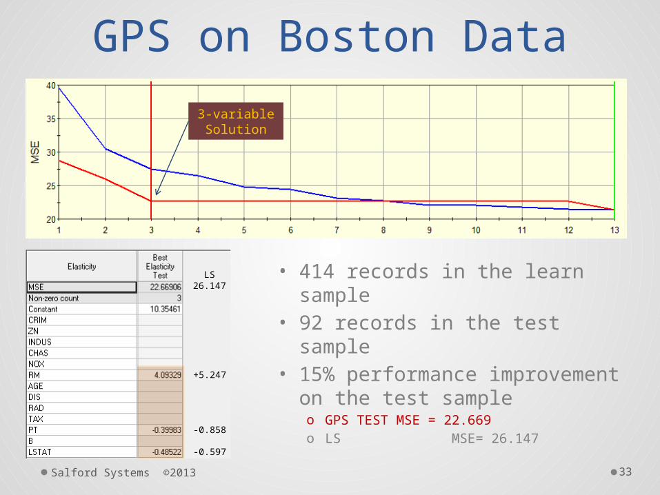
GPS on Boston Data
3-variable Solution
• 414 records in the learn sample
• 92 records in the test sample• 15% performance
improvement on the test sampleo GPS TEST MSE = 22.669o LS MSE= 26.147
+5.247
-0.858
-0.597
LS26.147
Salford Systems ©2013 34
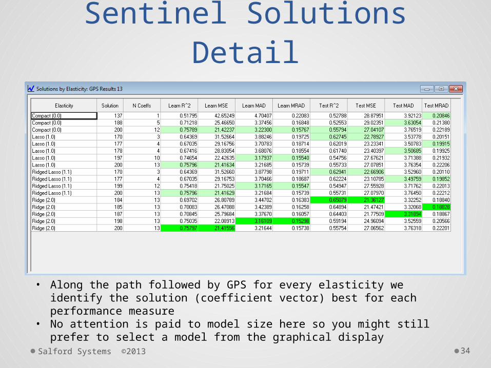
Sentinel Solutions Detail
• Along the path followed by GPS for every elasticity we identify the solution (coefficient vector) best for each performance measure
• No attention is paid to model size here so you might still prefer to select a model from the graphical display

Salford Systems ©2013 35
Regularized Logistic RegressionAll the same GPS ideas apply
Specify Logistic Binary Analysis
Specify optimality criterion

Salford Systems ©2013 36
How To Select a Best Model• Regularized regression was originally invented to
help modelers obtain more intuitively acceptable models
• Can think of the process as a search engine generating predictive models
• User can decide based on o Complexity of modelo Acceptability of coefficients magnitude, signs, predictors included)
• Clearly can be set to automatic mode• Criterion could well be performance on test data
Salford Systems ©2013 37
Key Problems with GPS• Still a linear regression!• Response surface is still a global hyper-plane• Incapable of discovering local structure in the
data
• Develop non-linear algorithms that build response surface locally based on the data itselfo By trying all possible data cuts as local boundarieso By fitting first-order adaptive splines locallyo By exploiting regression trees and their ensembles
Salford Systems ©2013 38
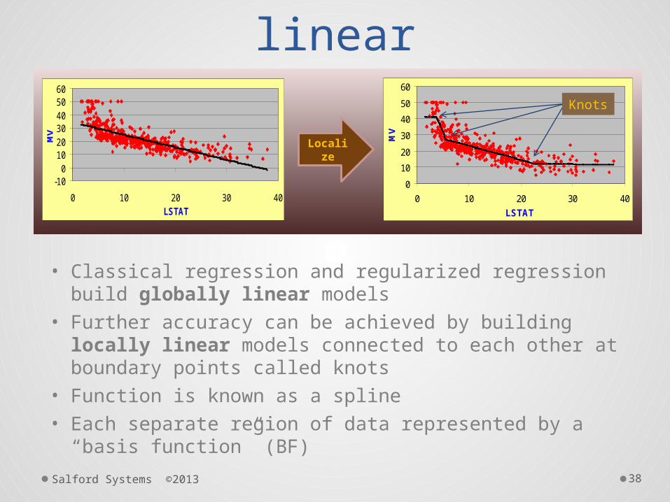
From Linear to Non-linear
• Classical regression and regularized regression build globally linear models
• Further accuracy can be achieved by building locally linear models connected to each other at boundary points called knots
• Function is known as a spline• Each separate region of data represented by a “basis
function” (BF)
-100
102030405060
0 10 20 30 40LSTAT
MV
0
10
20
30
40
50
60
0 10 20 30 40
LSTAT
MV
Localize
Knots
Salford Systems ©2013 39
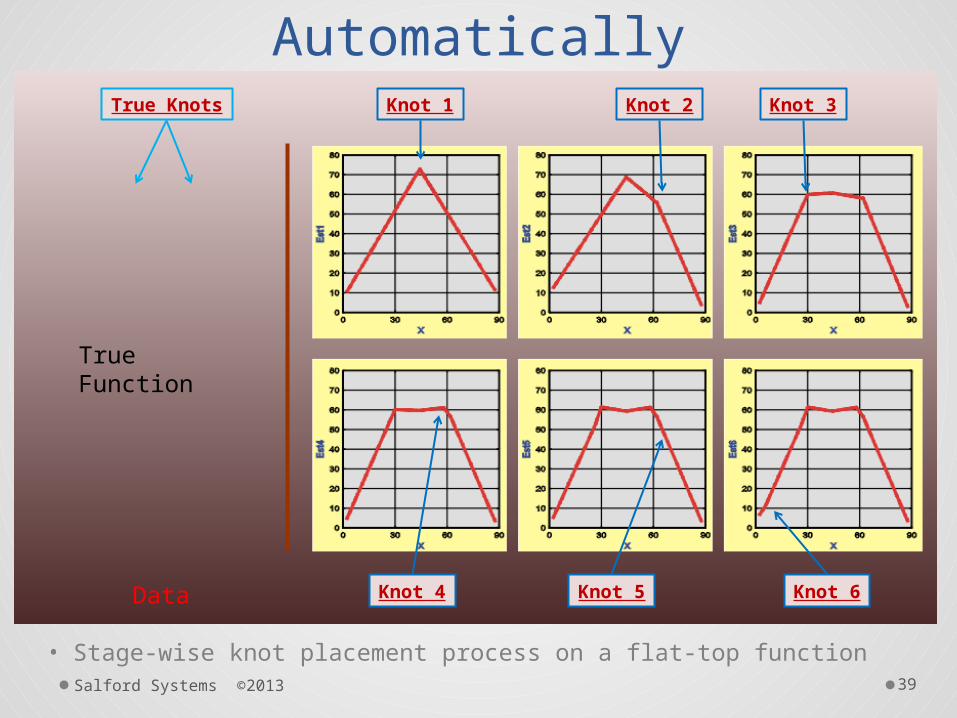
Finding Knots Automatically
• Stage-wise knot placement process on a flat-top function
True Knots Knot 1 Knot 2 Knot 3
Knot 4 Knot 5 Knot 6Data
True Function

Salford Systems ©2013 40
MARS Algorithm• Multivariate Adaptive Regression Splines• Introduced by Jerome Friedman in 1991
o (Annals of Statistics 19 (1): 1-67) (earlier discussion papers from 1988)
• Forward stage:o Add pairs of BFs (direct and mirror pair of basis functions represents a
single knot) in a step-wise regression mannero The process stops once a user specified upper limit is reached
• Backward stage:o Remove BFs one at a time in a step-wise regression mannero This creates a sequence of candidate models of declining complexity
• Selection stage:o Select optimal model based on the TEST performance (modern approach)o Select optimal model based on GCV criterion (legacy approach)
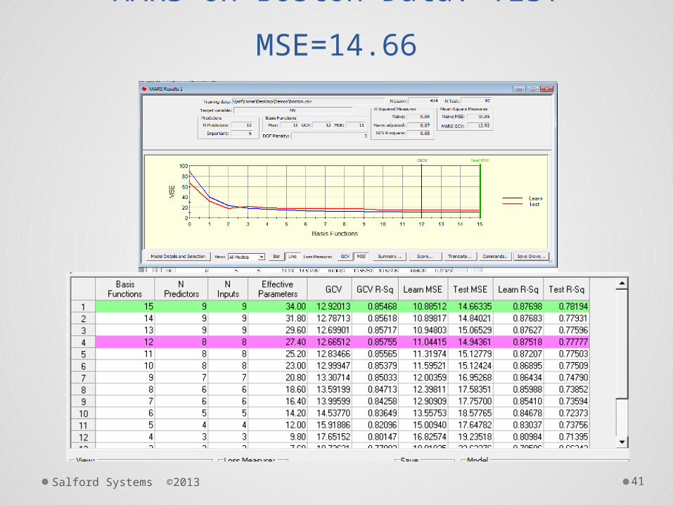
Salford Systems ©2013 41
MARS on Boston Data: TEST
MSE=14.66
9-BF (7-variable) Solution

Salford Systems ©2013 42
Non-linear Response Surface
• MARS automatically determined transition points between various local regions
• This model provides major insights into the nature of the relationship• Observe in this model NOX appears linearly

Salford Systems ©2013 43
200 Replications Learn/Test
Partition
• Models were repeated with 200 randomly selected 20% test partitions
• GPS shows marginal performance improvement but much smaller model
• MARS shows dramatic performance improvement
Regression
GPS
MARS
Distribution of TEST MSE across runs
Salford Systems ©2013 44
Combining MARS and GPS
• Use MARS as a search engine to break predictors into ranges reflecting differences in relationship between target and predictors
• MARS also handles missing values with missing value indicators and interactions for conditional use of a predictor (only when not missing)
• Allow the MARS model to be large• GPS can then select basis functions and shrink
coefficients• We will see that this combination of the best of
both worlds will also apply to ensembles of decision trees

Salford Systems © Copyright 2005-2013
45
Running Score: Test Sample MSEMethod 20%
randomParametric Bootstrap
Battery Partition
Regression 27.069 27.97 23.80
MARS Regression Splines
14.663 15.91 14.12
GPS Lasso/ Regularized
21.361 21.11 23.15

Salford Systems © Copyright 2005-2013
46
Regression TreeOut of the box results, no tuning of
controls
9 regions (terminal nodes)
Test MSE= 17.296
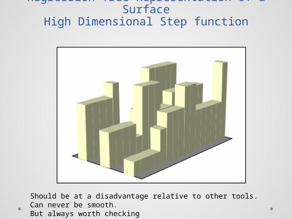
Regression Tree Representation of a Surface
High Dimensional Step function
Should be at a disadvantage relative to other tools. Can never be smooth.But always worth checking

Regression Tree Partial Dependency
Plot
LSTAT NOX
Use model to simulate impact of a change in predictorHere we simulate separately for every training data record and then averageFor CART trees is essentially a step functionMay only get one “knot” in graph if variable appears only once in tree
See appendix to learn how to get these plots
Salford Systems © Copyright 2005-2013
49
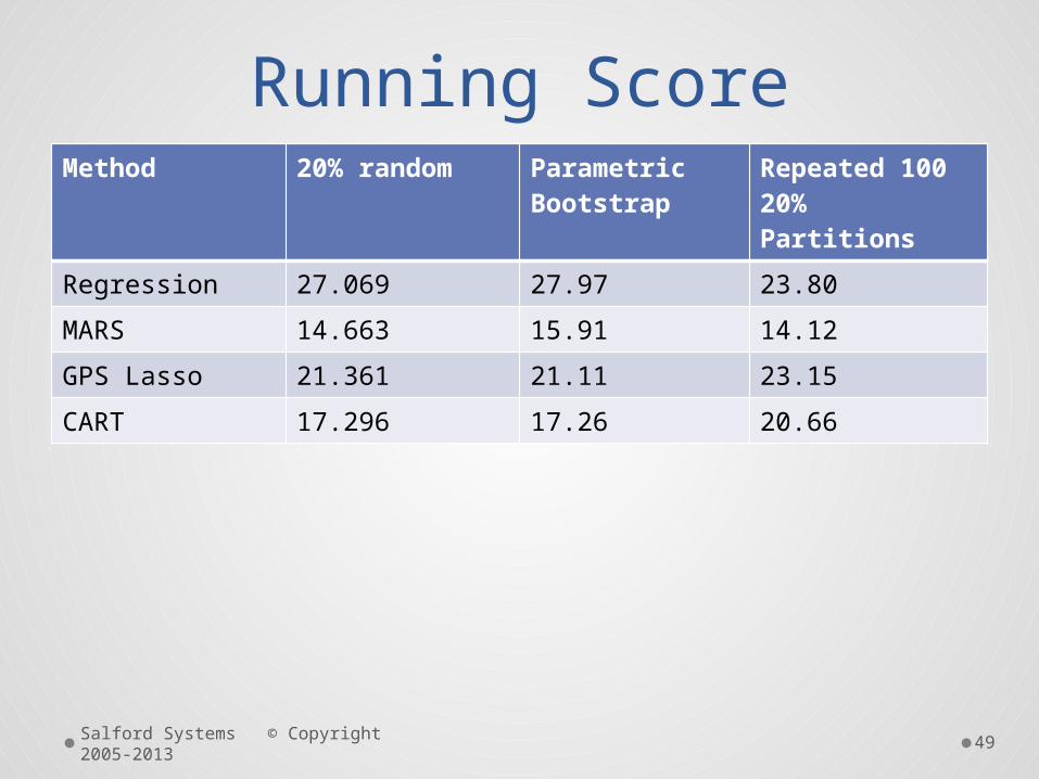
Running ScoreMethod 20% random Parametric
BootstrapRepeated 100 20% Partitions
Regression 27.069 27.97 23.80
MARS 14.663 15.91 14.12
GPS Lasso 21.361 21.11 23.15
CART 17.296 17.26 20.66

Salford Systems © Copyright 2005-2013
50
Bagger Mechanism• Generate a reasonable number of bootstrap samples
o Breiman started with numbers like 50, 100, 200
• Grow a standard CART tree on each sample• Use the unpruned tree to make predictions
o Pruned trees yield inferior predictive accuracy for the ensemble
• Simple voting for classificationo Majority rule voting for binary classificationo Plurality rule voting for multi-class classificationo Average predicted target for regression models
• Will result in a much smoother range of predictionso Single tree gives same prediction for all records in a terminal nodeo In bagger records will have different patterns of terminal node results
• Each record likely to have a unique score from ensemble
Salford Systems © Copyright 2005-2013
51
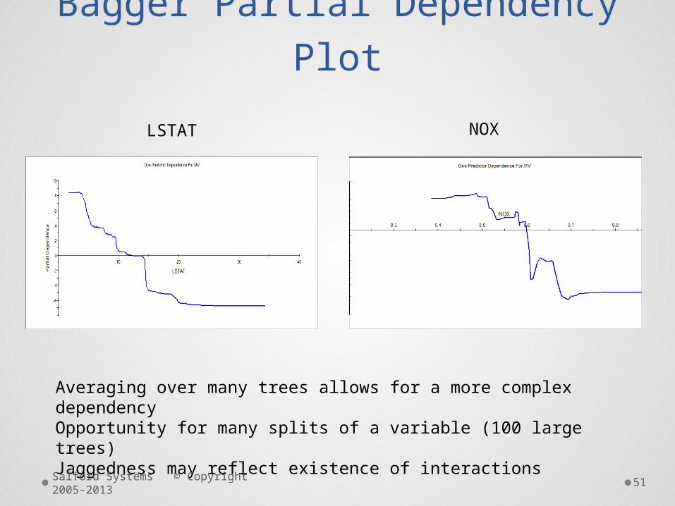
Bagger Partial Dependency Plot
LSTAT NOX
Averaging over many trees allows for a more complex dependencyOpportunity for many splits of a variable (100 large trees)Jaggedness may reflect existence of interactions
Salford Systems © Copyright 2005-2013
52
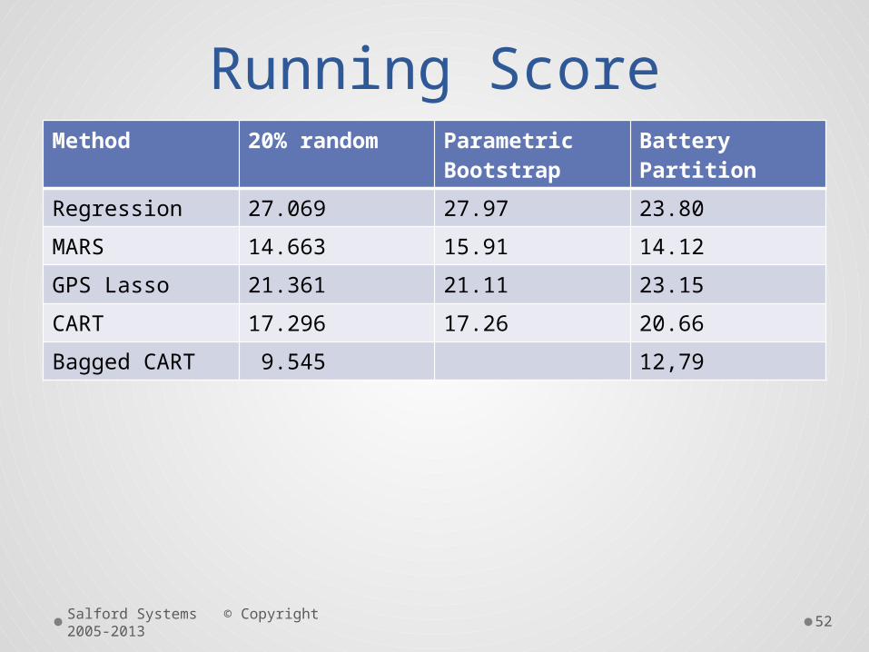
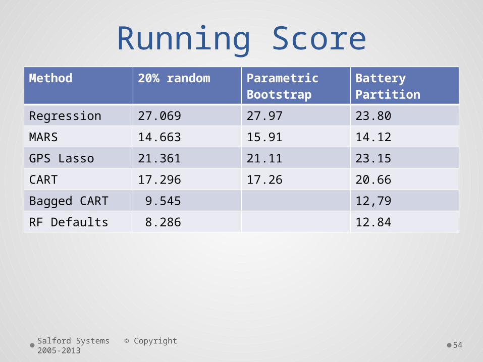
Running ScoreMethod 20% random Parametric
BootstrapBattery Partition
Regression 27.069 27.97 23.80
MARS 14.663 15.91 14.12
GPS Lasso 21.361 21.11 23.15
CART 17.296 17.26 20.66
Bagged CART 9.545 12,79
Salford Systems © Copyright 2005-2013
53
RandomForests: Bagger on
Steroids
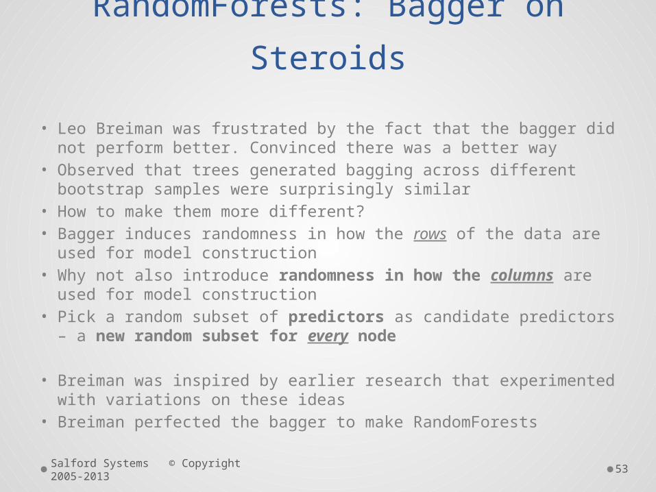
• Leo Breiman was frustrated by the fact that the bagger did not perform better. Convinced there was a better way
• Observed that trees generated bagging across different bootstrap samples were surprisingly similar
• How to make them more different?• Bagger induces randomness in how the rows of the data are
used for model construction• Why not also introduce randomness in how the columns are
used for model construction• Pick a random subset of predictors as candidate predictors – a
new random subset for every node
• Breiman was inspired by earlier research that experimented with variations on these ideas
• Breiman perfected the bagger to make RandomForests
Salford Systems © Copyright 2005-2013
54
Running ScoreMethod 20% random Parametric
BootstrapBattery Partition
Regression 27.069 27.97 23.80
MARS 14.663 15.91 14.12
GPS Lasso 21.361 21.11 23.15
CART 17.296 17.26 20.66
Bagged CART 9.545 12,79
RF Defaults 8.286 12.84

Salford Systems © Copyright 2005-2013
55
Stochastic Gradient Boosting (TreeNet )
• SGB is a revolutionary data mining methodology first introduced by Jerome H. Friedman in 1999
• Seminal paper defining SGB released in 2001o Google scholar reports more than 1600 references to this paper and a further
3300 references to a companion paper
• Extended further by Friedman in major papers in 2004 and 2008 (Model compression and rule extraction)
• Ongoing development and refinement by Salford Systemso Latest version released 2013 as part of SPM 7.0
• TreeNet/Gradient boosting has emerged as one of the most used learning machines and has been successfully applied across many industries
• Friedman’s proprietary code in TreeNet

Trees incrementally revise predictions
First tree grown on original target. Intentionally “weak” model
2nd tree grown on residuals from first. Predictions made to improve first tree
3rd tree grown on residuals from model consisting of first two trees
+ +
Tree 1 Tree 2 Tree 3
Every tree produces at least one positive and at least one negative node. Red reflects a relatively large positive and deep blue reflects a relatively negative node. Total “score” for a given record is obtained by finding relevant terminal node in every tree in model and summing across all trees
Salford Systems © Copyright 2005-2013
56

Salford Systems © Copyright 2005-2013
57
Gradient Boosting Methodology: Key
points
• Trees are usually kept small (2-6 nodes common)o However, should experiment with larger trees (12, 20, 30
nodes)
o Sometimes larger trees are surprisingly good
• Updates are small (downweighted). Update factors can be as small as .01, .001, .0001. o Do not accept the full learning of a tree (small step size, also GPS
style)
o Larger trees should be coupled with slower learn rates
• Use random subsets of the training data in each cycle. Never train on all the training data in any one cycleo Typical is to use a random half of the learn data to grow each tree

Salford Systems © Copyright 2005-2013
58
Running ScoreMethod 20% random Parametric
BootstrapBattery Partition
Regression 27.069 27.97 23.80
MARS 14.663 15.91 14.12
GPS Lasso 21.361 21.11 23.15
CART 17.296 17.26 20.66
Bagged CART 9.545 12,79
RF Defaults 8.286 12.84
RF PREDS=6 8.002 12.05
TreeNet Defaults
7.417 8.67 11.02
Using cross-validation on learn partition to determine optimal number of trees and then scoring the test partition with that model: TreeNet MSE=8.523
Salford Systems © Copyright 2005-2013
59
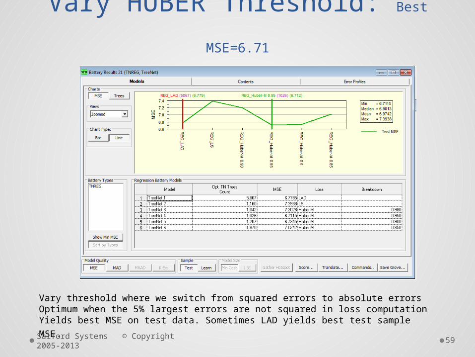
Vary HUBER Threshold: Best
MSE=6.71
Vary threshold where we switch from squared errors to absolute errorsOptimum when the 5% largest errors are not squared in loss computation
Yields best MSE on test data. Sometimes LAD yields best test sample MSE.
Salford Systems © Copyright 2005-2013
60
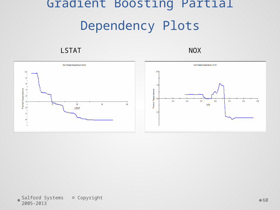
Gradient Boosting Partial Dependency
Plots
LSTAT NOX
Salford Systems © Copyright 2005-2013
61
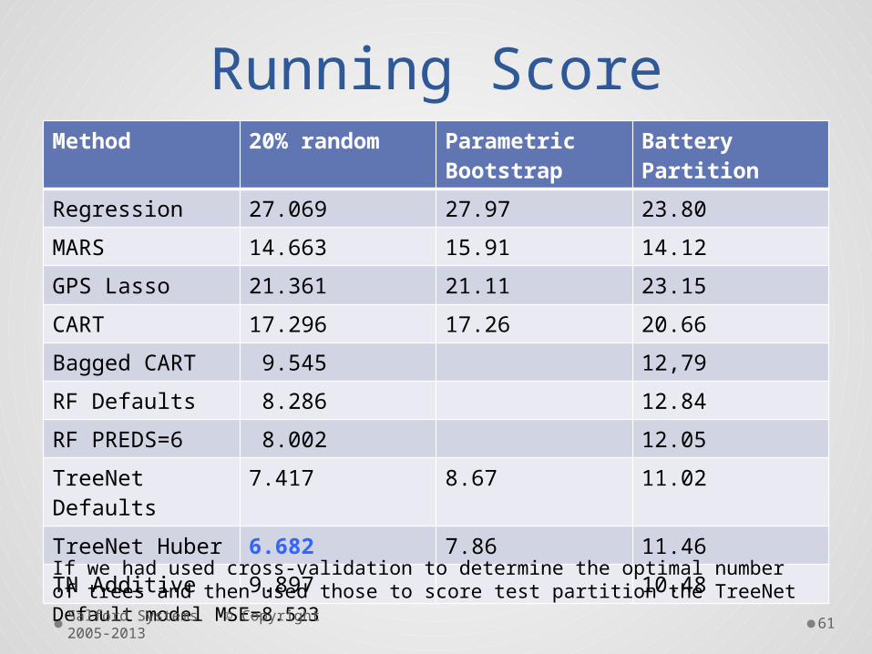
Running ScoreMethod 20% random Parametric
BootstrapBattery Partition
Regression 27.069 27.97 23.80
MARS 14.663 15.91 14.12
GPS Lasso 21.361 21.11 23.15
CART 17.296 17.26 20.66
Bagged CART 9.545 12,79
RF Defaults 8.286 12.84
RF PREDS=6 8.002 12.05
TreeNet Defaults
7.417 8.67 11.02
TreeNet Huber 6.682 7.86 11.46
TN Additive 9.897 10.48If we had used cross-validation to determine the optimal number of trees and then used those to score test partition the TreeNet Default model MSE=8.523

Salford Systems ©2013 62
References MARS
• Friedman, J. H. (1991a). Multivariate adaptive regression splines (with discussion). Annals of Statistics, 19, 1-141 (March).
• Friedman, J. H. (1991b). Estimating functions of mixed ordinal and categorical variables using adaptive splines. Department of Statistics,Stanford University, Tech. Report LCS108.
• De Veaux R.D., Psichogios D.C., and Ungar L.H. (1993), A Comparison of Two Nonparametric Estimation Schemes: Mars and Neutral Networks, Computers Chemical Engineering, Vol.17, No.8.

Salford Systems ©2013 63
References Regularized
Regression
• Arthur E. HOERL and Robert W. KENNARD. Ridge Regression: Biased Estimation for Nonorthogonal Problems TECHNOMETRICS, 1970, VOL. 12, 55-67
• Friedman, Jerome. H. Fast Sparse regression and Classification. http://www-stat.stanford.edu/~jhf/ftp/GPSpaper.pdf
• Friedman, J. H., and Popescu, B. E. (2003). Importance sampled learning ensembles. Stanford University, Department of Statistics. Technical Report. http://www-stat.stanford.edu/~jhf/ftp/isle.pdf
• Tibshirani, R. (1996). Regression shrinkage and selection via the lasso. J. Royal. Statist. Soc. B. 58, 267-288.

Salford Systems ©2013 64
References Regression via Trees
• Breiman, L., J. Friedman, R. Olshen and C. Stone (1984), Classification and Regression Trees, CRC Press.
• Breiman, L (1996), Bagging Predictors, Machine Learning, 24, 123-140
• Breiman, L. (2001) Random Forests. Machine Learning. 45, pp 5-32.
• Friedman, J. H. Greedy function approximation: A gradient boosting machine http://www-stat.stanford.edu/~jhf/ftp/trebst.pdf Ann. Statist. Volume 29, Number 5 (2001), 1189-1232.
• Friedman, J. H., and Popescu, B. E. (2003). Importance sampled learning ensembles. Stanford University, Department of Statistics. Technical Report. http://www-stat.stanford.edu/~jhf/ftp/isle.pdf

Salford Systems ©2013 65
What’s Next• Visit our website for the full 4-hour video series• https://www.salford-systems.com/videos/tutorials/the-
evolution-of-regression-modeling o 2 hours methodologyo 2 hours hands-on running of exampleso Also other tutorials on CART, TreeNet gradient boosting
• Download no-cost 60-day evaluationo Just let the Unlock Department know you participated in the on-demand
webinar series
• Contains many capabilities not present in open source renditionso Largely the source code of the inventor of today’s most important data
mining methods: Jerome H. Friedmano We started working with Friedman in 1990 when very few people were
interested in his work

© Salford Systems 2012
Salford Predictive Modeler SPM
• Download a current version from our website http://www.salford-systems.com
• Version will run without a license key for 10-days
• For more time request a license key [email protected]
• Request configuration to meet your needso Data handling capacityo Data mining engines made available