evolution strategies for the next generation passive optical networks
TRANSCRIPT

Evolution Strategies for the Next Generation Passive Optical
Networks
Jorge Manuel Patrocínio Galveias
Dissertation to obtain the degree of
Master in Electrical and Computer Engineering
Jury
President: Prof. Fernando Duarte Nunes
Supervisor : Prof. João José de Oliveira Pires
Co- Advisor : António Miguel Barata Da Eira
Members : Prof. Armando Humberto Moreira Nolasco Pinto
October 2012

ii
Acknowledgements
First of all, I would like to thank Professor João Pires for all the patience and time, Antório Eira, of
Nokia Siemens Networks, for his absolutely crucial help at the start of this Thesis.
I want to thank my family, for having contributed for the person I am, my father, Jorge Rodrigues
Galveias, for teach me that life was not meant to be easy, my mother, Margarida Patrocínio, for the
sweetness and affection, my grandmother, Maria Amélia Rodrigues, for the lessons and affection, all my
uncles, specially, Luis Galveias and Paulo Galveias, for the link that has connected us from the day I was
born, my cousins, specially, Rodrigo Matafome Galveias, João Paulo Galveias and Susana Galveias
Santos.
A special word to my grandmother for all the care she has given to every single member of our
family, for the permanent state of affection towards us, for the smiles, for the lessons, and for much much
more, thank you very much dear grandmother.
I would like to thank all my friends, specially Luis Ribeiro, José Marona and Maria Fonseca, for
all the moments we´ve spent together and thing they have taught me.
Finally, I want to say a special word to Ana, just to tell her that she is the one my heart cares about.

iii
Abstract
In the near future, current passive optical networks (PONs) will need capacity upgrades
due to the increasing demand by customers. More precisely, the existing wavelength channels
may need to be upgraded or/and other wavelengths may need to be added.
This thesis makes an extensive use of integer linear programming (ILP) formulations
alongside with pricing policies for optical receivers and transmitters in order to understand what
will be the cost of the next generation passive optical networks and the required bandwidth per
wavelength channel. Each ILP formulation runs under a multi-period simulation, in which from
period to period the traffic of the network´s upstream channels increase by a certain value.
The study begins by analyzing an hybrid TDM/WDM PON using a previously published
ILP formulation. Such formulation is extended and three ILP models were developed, in order to
study the network behavior when tunable lasers are used in the ONUs as well as a CWDM grid.
Two of the models use channels working at 10 Gbps, whereas in the other one the channels
can work at 10 or 40 Gbps. In each simulation setup, the network is studied with 16, 32 and 64
ONUs, as well as tunable lasers with 2, 4 and 8 wavelengths.
The last ILP model developed in this thesis considers one PON, which uses an arrayed
waveguide grating (AWG) with a range of 32 DWDM channels at the central office and single
wavelength DWDM lasers working at 10 Gbps. Nine simulations are presented, resulting from
the combination of three number of ONUs in the PON (16, 32 and 64) and three number of
output ports of the AWG (4, 8 and 16).
Keywords : Hybrid TDM/WDM PON, CWDM, DWDM, AWG, Mixed Integer Linear Programming

iv
Resumo
Num futuro próximo, as redes ópticas passivas (PONs) necessitarão de serem
actualizadas devido ao crescente tráfego exigido pelos clientes destas redes. Em particular, os
canais ópticos existentes poderão precisar de serem actualizados ou/e novos canais ópticos
precisarão de ser adicionados.
Esta dissertação utiliza as formulações de programação linear inteira (ILP) em conjunto
com políticas de custo anexadas aos receptores e transmissores ópticos de forma a perceber
qual será o custo das redes passivas ópticas de nova geração e a largura de banda necessária
para cada canal de comprimento de onda. Cada formulação ILP usa uma simulação do tipo
multi período em que de período para período o trafego dos canais ascendentes das redes
aumenta por um determinado factor.
O estudo começou pela análise da rede híbrida TDM/WDM PON usando uma
formulação ILP de um artigo publicado anteriormente. O âmbito dessa formulação foi alargado
desenvolvendo-se três modelos por forma a perceber o comportamento da rede, em termos de
custo, quando se usam lasers sintonizáveis nos terminais ópticos dos clientes e se utilizava a
grelha CWDM. Dois desses modelos utilizavam canais ópticos a 10 Gbps enquanto num
terceiro modelo esses canais podiam funcionar a 10 Gbps ou a 40 Gbps. Em configuração de
simulação a rede é estudada com 16, 32 ou 64 ONUs e lasers sintonizáveis de 2,4 ou 8
comprimentos de onda.
O último modelo desenvolvido contempla uma PON que utiliza um equipamento,
denominado em Inglês arrayed waveguide grating (AWG), funcionando numa janela de 32
comprimentos de onda e usando uma grelha DWDM. Nove simulações são apresentadas, que
resultam da combinação de três números diferentes de ONUs na PON ( 16, 32 e 64 ) e três
números de portos de saída do AWG (4,8 and 16).
Palavras Chave: PON híbrida TDM/WDM, CWDM, DWDM, AWG, Programação Linear Inteira
v
Table of Contents
1. Introduction ............................................................................................................................ 1
1.1. Optical Access Networks ............................................................................................... 2
1.2. Next Generation Passive Optical Networks ..................................................................... 7
1.3. State Of the Art .............................................................................................................. 9
1.4. Motivation, Objectives and Structure ........................................................................... 11
1.5. Original Contributions ................................................................................................. 12
2. Migration Scenario to the Next Generation PON ................................................................ 13
3. Migration scenario reformulated .......................................................................................... 26
3.1. Wavelength grids ......................................................................................................... 27
3.5.1. Results for Model I ............................................................................................... 37
3.5.2. Results for Model II ............................................................................................. 43
3.5.3. Analysis ................................................................................................................ 48
3.6. Conclusion ................................................................................................................... 49
4. Moving towards the 40 Gbps technology ............................................................................ 50
4.2. MILP Model III ........................................................................................................... 52
4.3. Improving the Performance of the Model III ................................................................ 54
4.4. Results and discussion .................................................................................................. 60
4.5. Conclusion ................................................................................................................... 65
5. The AWG at the Access Level ............................................................................................ 66
5.1. Introducing the problematic ......................................................................................... 67
5.2. MILP Model Number IV .............................................................................................. 69
5.3. Results and Discussion.................................................................................................. 71
5.4. Conclusion ................................................................................................................... 75
6. Conclusions and Future Work .............................................................................................. 76
6.1. Conclusions .................................................................................................................. 76
6.2. Future Work ................................................................................................................ 77
References .................................................................................................................................. 78
A. Information about the simulation of the MILP Model IV ...................................................... 80

vi
List of Figures
Figure 1.1 – Hybrid fiber-coax network[3] ..................................................................................... 2 Figure 1.2 – Several Types of FTTx[3] Figure 1.3 - Point-to-Point FTTH network[5] ................. 3 Figure 1.4 – P2P Ethernet FTTH network[3] ................................................................................. 4 Figure 1.5 – Architecture of a typical passive optical network (PON) ........................................... 5 Figure 1.6 - Wavelength allocation pattern for 10GEPON [16] ..................................................... 8 Figure 1.7 - XG-PON architecture[20] ........................................................................................... 8 Figure 1.8 - XG-PON and GPON wavelength band representation [20]....................................... 8 Figure 1.9 – a) legacy PON, b) partial upgrade for 10G-PON, c) extending capacity by adding
downstream (and/or upstream) channel to a set of ONUs, d) extending capacity by adding more
channels to sets of ONUs as needed[21] .................................................................................... 10 Figure 2.1 - Hybrid TDM/WDM PON (upstream perspective) ..................................................... 14 Figure 2.2 – Simulation´s flowchart ............................................................................................. 18 Figure 2.3 - Number of wavelengths assigned to the PON per period and its total traffic
occupation in Mbps for 16 ONUs ................................................................................................ 21 Figure 2.5 – the same information given by Table 2.1 but directly from [24] .............................. 24 Figure 2.4 - Same information given by Figure 2.3 but taken directly from [24] ......................... 24 Figure 3.1 - Distribution of the wavelengths per lasers, using lasers of two, four and eight
wavelengths (Model One) ........................................................................................................... 29 Figure 3.2 - Number of laser types, five (but only 3 are represented in the figure), for eigth
wavelength channels and four wavelengths per laser (Second Model) ...................................... 29 Figure 3.3 - Flowchart for the simulation of the model one and two ........................................... 34 Figure 3.4 - Graphic information about the introduction of receivers .......................................... 36 Figure 3.5 - Cost and Number of upgrading ONUs along the time for the Model I at 16 ONUs . 37 Figure 3.6 - Percentage of bandwidth allocated along time for the Model I at 16 ONUs ............ 38 Figure 3.7 - Cost and Number of upgrading ONUs along the time for the Model I at 32 ONUs . 39 Figure 3.8 - Percentage of bandwidth allocated along time for the Model I at 32 ONUs ............ 40 Figure 3.9 - Cost and Number of upgrading ONUs along the time for the Model I at 64 ONUs . 40 Figure 3.10 - Percentage of bandwidth allocated along time for the Model I at 64 ONUs .......... 41 Figure 3.11 - Total Cost for the simulations of the Model I ......................................................... 42 Figure 3.12 - Cost and Number of upgrading ONUs along the time for the Model II at 16 ONUs
..................................................................................................................................................... 43 Figure 3.13 - Percentage of bandwidth allocated along time for the Model I at 16 ONUs .......... 44 Figure 3.14 - Cost and Number of upgrading ONUs along the time for the Model II at 32 ONUs
..................................................................................................................................................... 45 Figure 3.15 - Percentage of bandwidth allocated along time for the Model I at 32 ONUs .......... 46 Figure 3.16 - Cost and Number of upgrading ONUs along the time for the Model II at 64 ONUs
..................................................................................................................................................... 46 Figure 3.17 - Percentage of bandwidth allocated along time for the Model I at 64 ONUs .......... 47 Figure 3.18 - Total Cost for the simulations of the Model II ........................................................ 47 Figure 4.1 - Wavelength channels (Upstream wavelengths), data rates and Lasers, when each
tunable laser has two wavelengths per laser. ............................................................................. 51 Figure 4.2 – Algorithm´s new working flowchart ......................................................................... 56 Figure 4.3 – State Diagram for a simulation using Lp=4 with optimization ................................. 59 Figure 5.1 - AWG working as Multiplexer/Demultiplexer and Router .......................................... 67 Figure 5.2 - FSR cyclic pattern for a 32 wavelengths and 4 FSRs and M=8 .............................. 67 Figure 5.3 - Network Architecture................................................................................................ 68 Figure 5.4 - Average Load of the channels (Model IV) for 16 ONUs .......................................... 73 Figure 5.5 - Average Load of the channels (Model IV) for 32 ONUs .......................................... 73 Figure 5.6 - Average Load of the Channels (Model IV) for 64 ONUs ......................................... 74

vii
List of Tables
Table 1.1 – Power budget classes of the 10GEPON .................................................................... 8 Table 1.2 – XG-PON 1 information about the classes of the XG-PON1 ....................................... 9 Table 2.1 – wavelength allocation per ONU and period for the 1xTx mode and 16 ONUs
(Notation [x Mbps]λi, x upstream traffic demand by ONU i ; the bold text represents a new
wavelength at 10 Gbps in the ONU i, blue text represents wavelengths at 40 Gbps in the ONU i,
and bold blue text gathers the information of the blue and bold text already explained) ............ 20 Table 2.2 – Details about the simulation with 16 ONUs .............................................................. 22 Table 2.3 – Details about the simulation with 32 ONUs .............................................................. 22 Table 2.4 – Details about the simulation with 64 ONUs .............................................................. 23 Table 2.5 – Total Cost for 16, 32 and 64 ONUs in the PON ....................................................... 23 Table 3.1 – ITU-T G694.2 CWDM grid ........................................................................................ 28 Table 3.2 - Relative Cost of the Tunable lasers .......................................................................... 35 Table 3.3 - Relative cost of the receivers .................................................................................... 35 Table 3.4 - Cost Difference [Model I – Model II] between the model one and two, for the initial
values of Z and W ....................................................................................................................... 48 Table 4.1 – ONU costs for the model III ...................................................................................... 61 Table 4.2 – OLT costs for the model III ....................................................................................... 61 Table 4.3 - Information about the simulation with 16 Onus. ........................................................ 62 Table 4.4 - Information about the simulation with 32 ONUs ....................................................... 63 Table 4.5 - Information about the simulation with 64 ONUs ....................................................... 63 Table 4.6 – Ratio Between the 40 Gbps side and the 10 Gbps side of the simulations ............. 64 Table 5.1 - Equipment OPEX and CAPEX costs ........................................................................ 71 Table 5.2 - Simulation Cases ...................................................................................................... 72 Table 5.3 – Simulation Results(Model IV) for 16 ONUs .............................................................. 72 Table 5.4 – Simulation Results (Model IV) for 32 ONUs ............................................................. 72 Table 5.5 – Simulation Results (Model IV) for 64 ONUs ............................................................. 73 Table A.1 – Simulation information, M=4 and 16 ONUs (Model IV) ........................................... 80 Table A.2 - Simulation information, M=8 and 16 ONUs (Model IV) ............................................ 81 Table A.3 - Simulation information, M=16 and 16 ONUs (Model IV) .......................................... 81 Table A.4 - Simulation information, M=4 and 32 ONUs (Model IV) ............................................ 82 Table A.5 - Simulation information, M=8 and 32 ONUs (Model IV) ............................................ 82 Table A.6 - Simulation information, M=16 and 32 ONUs (Model IV) .......................................... 83 Table A.7 - Simulation information, M=4 and 64 ONUs (Model IV) ............................................ 83 Table A.8 - Simulation information, M=8 and 64 ONUs (Model IV) ............................................ 84 Table A.9 - Simulation information, M=16 and 64 ONUs (Model IV) .......................................... 84

viii
List of Acronyms
APON – ATM Passive Optical Network
AWG- Arrayed Waveguide Grating
BPON – Broadband Passive Optical Network
CAPEX – Capital Expenditure
CD – Chromatic Dispersion
CWDM – Coarse Wavelength Division Multiplexing
DML – Directly Modulated Laser
DQPSK – Differential quadrature phase shift keying
DWDM - Dense Wavelength Division Multiplexing
EML – Externally Modulated Laser
EPON – Ethernet Passive Optical Network
FEC – Forward Error Correction
FP – Fabry-Perot
FSAN – Full Service Access Networks
FSR- Free Spectral Range
PON – Passive Optical Network
FTTB –Fibre-To-The-Building
FTTC – Fibre-To-The-Curb
FTTH – Fibre-To-The-Home
FTTN – Fibre-To-The-Node
GEM – Generic Encapsulation Method
GEPON – The same as EPON
GPON – Gigabit Passive Optical Network
GTC – GPON Transmission convergence
ILP – Integer Linear Programming
LAN – Local Area Network
MILP -Mixed Integer Linear Programming
MAN- Metropolitan Area Network
MDU – Multi-Dwelling Unit
NRZ – Non Return to Zero
ODN- Optical Distribution Network
ONT- Optical Network Terminal

ix
ONU- Optical Network Unit
OPEX – Operational Expenditure
P2MP – Point-To-Multipoint
P2P – Point-to-Point
PMD – Polarization Mode Dispersion
PON – Passive Optical Network
SDO – Standards Development Organization
TDM – Time Division Multiplexing
TDMA - Time Division Multiple Access
VLAN – Virtual LAN
WAN – Wide Area Network
WBF – Wavelength Blocking Filter
WDM – Wavelength Division Multiplexing

1
1. Introduction
In this chapter, the access network will be revisited from the beginning of its existence,
how it evolved and how and when fiber was introduced in it. Then, current passive optical
networks will be analyzed and compared. Finally, the state of the art, the objectives and
structure of the thesis are presented.

2
1.1. Optical Access Networks
Fiber optics have been deployed in the core and metro networks since 1977 [1], when the
first generation of optical fiber appeared. Before that period, networks, including the access
networks, were based on twisted pairs and coaxial cables, both made out of copper.
Firstly, access networks were responsible for delivering telephone services, so called
plain old telephone services (POTS), and cable television services (CATV). Each service had its
own network, but both networks had a tree topology.
The POTS operated over a twisted pair network, whereas the CATV operated using a
coaxial cable network, the so called one-way CATV plant, since it only had the downstream
signal to broadcast the video towards subscribers. In the early 1990´s the Digital Subscriber
Line (DSL) technology appeared, reusing the infrastructure of the POTS to provide both
telephone and data services, such as internet. With the increase of web pages multimedia
content, several flavours of DSL technologies[2] have been developed, of which the Asymmetric
Digital Subscriber Line (ADSL1) and Very-high-bit-rate Digital Subscriber Line (VDSL
2) are the
most common ones.
Still in the early 1990´s, the introduction of optical fiber in the CATV network in its trunk
side was done to minimize the noise produced by long amplifier cascades used in the previous
CATV system. Consequently, the Hybrid Fiber Coaxial (HFC) network was born, replacing the
old all coaxial CATV system, and soon afterwards it was provided an upstream channel which
supports the pay-per-view and video-on-demand services. Later on, in 1997, the DOCSIS 1.03
was introduced in the HFC network aiming high-speed data transfer, used by many operators to
provide internet service over cable.
Figure 1.1 – Hybrid fiber-coax network[3]
According to Figure 1.1, an HFC network includes two parts. The first part one denoted
as super-truck extends from the optical headend to the Optical-to-electrical service node, which
can measure from five up to forty kilometers. The second part of that network, from the service
node to the subscriber, uses coaxial cable and contains the coaxial trunk, the feeder and drop
cables, which define a tree topology and serve up to 2000 houses. To compensate the cable
attenuation over long distance in that part of the network, several RF amplifiers are used along
1ADSL : up 8 Mbps in the downstream and up 800 Kbps in the upstream over a distance of 5.5 Km[2]
2VDSL : up to 52 Mbps in the downstream and up to 16 Mbps in the upstream over a distance of 1.2 Km
[2] 3 The latest version of DOCSIS is the 3.0, which provides up 160 Mbps in the downstream an 120 Mbps in
the upstream[2]
3
the way. The coaxial part of the network has a main trunk leaving the service node heading to
the residential/business area of interest. There, the trunk cable ends in a splitter, from where
several feeder cables begin their course towards streets. An RF4 tag is used to extract the
signal from the feeder cable to the drop cable, which is connected to the clients´ equipment
such as TV, computer, et cetera.
Internet has ruled, since 1990, when the World-Wide-Web was created, the increase of
bandwidth demanded by customers due to the online services and multimedia content emerging
from this platform, such as e-commerce, e-learning, IPTV, video streaming, file transferring and
peer-to-peer. All the internet services and other data communications services have influenced
an overall growth on average of about 50 percent per year with respect to the access network´s
traffic[4].
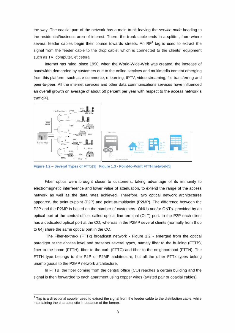
Figure 1.2 – Several Types of FTTx[3] Figure 1.3 - Point-to-Point FTTH network[5]
Fiber optics were brought closer to customers, taking advantage of its immunity to
electromagnetic interference and lower value of attenuation, to extend the range of the access
network as well as the data rates achieved. Therefore, two optical network architectures
appeared, the point-to-point (P2P) and point-to-multipoint (P2MP). The difference between the
P2P and the P2MP is based on the number of customers- ONUs and/or ONTs- provided by an
optical port at the central office, called optical line terminal (OLT) port. In the P2P each client
has a dedicated optical port at the CO, whereas in the P2MP several clients (normally from 8 up
to 64) share the same optical port in the CO.
The Fiber-to-the-x (FTTx) broadcast network - Figure 1.2 - emerged from the optical
paradigm at the access level and presents several types, namely fiber to the building (FTTB),
fiber to the home (FTTH), fiber to the curb (FTTC) and fiber to the neighborhood (FTTN). The
FTTH type belongs to the P2P or P2MP architecture, but all the other FTTx types belong
unambiguous to the P2MP network architecture.
In FTTB, the fiber coming from the central office (CO) reaches a certain building and the
signal is then forwarded to each apartment using copper wires (twisted pair or coaxial cables).
4 Tap is a directional coupler used to extract the signal from the feeder cable to the distribution cable, while
maintaining the characteristic impedance of the former.

4
In the FTTC and FTTB, the fiber reaches the optical network unit (ONU), where the
signal is converted from optical to electrical. In the FTTC the ONU is placed within less than 300
meters of the residential/business area of interest, whereas in the FTTN the ONU is placed
within one kilometer of the customer. Often, the copper side of the FTTC contains a VSDL
connection, taking advantage of the sort distance from the ONU to the customer to provide a
high data rate link. Finally, in the FTTH, the path between the CO and the customer - optical
network unit (ONU) - is done exclusively by fiber.
Figure 1.4 – P2P Ethernet FTTH network[3]
Usually, the technology applied in P2P architectures is the Ethernet, working at 100
Mbps,1 Gbps or 10 Gbps. The downstream voice, data and video services are combined into a
single wavelength as well as the upstream communication - Figure 1.4. The P2P architecture
has a problem related with the number of transceivers5 needed. N clients require 2N
transceivers, N in the OLT and one per each client. Regarding the P2MP architectures, two
major implementations are considered, namely the active star (AON) and the passive star
(PON). In the former, the remote node is a point of traffic aggregation, such as an Ethernet
switch, whereas the latter has a power splitter/combiner in the remote node, which has the
advantage of having no need for power supply.
The passive star networks, so called passive optical networks, are the most efficient
regarding the usage of transceivers, since only N+1 transceivers are needed to provide service
to N clients, unlike the P2P and P2MP active networks that need 2N and 2N+2 transceivers,
respectively.
However, the more transceivers being used, the more bandwidth the network can
provide. So the P2P networks can easily provide 100 Mbps or 1 Gbps dedicated bandwidth, on
both direction of communication whereas the bandwidth per client in PONs depends on the
number of clients. Still, the PON networks lower OPEX and CAPEX costs compared with other
optical networks made this network the most adapted all over the world when upgrading the old
access networks to an optical one.
5 Single device that is responsible for both signal transmission and receiving processes

5
Figure 1.5 – Architecture of a typical passive optical network (PON)
PONs are an implementation of a P2MP passive architecture and work with two or three
wavelengths. The signal leaving the OLT port reaches the power splitter and there each output
port gets a replica, with lower power, of the original optical signal. The power splitter has an
intrinsic splitter factor (1: N), which depends on the number of ONTs/ONUs we want to provide
service (N is normally a power of two). Consequently, each replica has less than 1 over N of the
original power transmitted by the OLT reaching the remote node.
Regarding the upstream communication, the wavelength is shared in time by the
ONUs/ONTs. This means a time division multiple access (TDMA) protocol must run at the same
time the communication is done. In fact, not all PON types use the same TDMA protocol, but
such protocols a common working philosophy. Each ONU is given timeslots where it can
transmit its traffic and such allocation can be done in a dynamic or fixed manner depending on
the utilization or not of a dynamic bandwidth allocation (DBA) algorithm at the OLT6.
Several PONs have been standardized and deployed since 1995. In fact, the first PON
developed was TPON in 1989, but its major purpose was to give researchers the information
about such advance access implementation, at the time. After the success of the trial
deployment of the TPON, researchers recognized it would be a good idea to implement an
ATM-based service over a passive optical network. Therefore APON began its standardization
in 1995 and took 2 years to be concluded, developed by the Full Service Access Network
(FSAN) group which belongs to the Telecommunication Standardization Sector of the
International Telecommunication Union (ITU-T). APON [6] stands for ATM passive Optical
Network and as the name suggests, uses the asynchronous transfer mode cell as its basic unit
of communication, having a 5 bytes header and 48 bytes payload, in a total of 53 bytes. The
power splitter used can link 16 or 32 clients, depending on the distance the PON is covering.
The downstream wavelength is allocated in the C band, centered at 1490 nm, the upstream one
is using the O band centered at 1390 nm, and both wavelengths are working at 155 Mbit/s.
APON has no DBA algorithm, this means the timeslots allocation is done in a fixed manner.
The Broadcast Passive Optical Network(BPON) [7–9] is the evolution of APON, and uses
ATM cells as well. The recommendations for the BPON are the G983.3, G983.4 and G983.5,
which have introduced some major features not present in the APON. First of all, BPON
introduced the video broadcast service, at the 1550 nm wavelength, using the wavelength
division multiplexing method in the downstream direction. Secondly, the communication data
6 PONs work in a master slave fashion where the master is the OLT and the slave is the ONU or ONT, and
so the OLT is the equipment that decides when the ONUs/ONTs can use the uplink

6
rate was raised in both directions, the downlink may work at up to 1.24 Gbit/s and the uplink up
to 622 Mbit/s. Thirdly, the dynamic bandwidth allocation algorithms were introduced to increase
the upstream channel usage as well as to increase the quality of service.
Gigabit passive optical network (GPON) [10–13], following the BPON, was proposed by
the FSAN/ITU-T group in the G984 recommendations, and have been deployed throughout the
United States of America and Europe. It is capable of working with data rates up to 2.4 Gbit/s, in
an asymmetrical manner, 2.4 Gbit/s in the downstream and 1.24 Gbit/s in the upstream, or in a
symmetrical manner, in which both communications work at 2.4 Gbit/s. However, the major
PONs deployment in the field use only the asymmetric implementation due to costs reduction at
ONU/ONT side. The range covered by this PON is 20 kilometers and the maximum split factor
was increased to 1:128, but the 1:64 split factor is more likely to be used, due to power budget7
constraints. By the time the GPON was developed, the ATM technology was starting to fade,
mainly due to its lack of efficiency when transporting non ATM traffic, and as an answer to this
fact the ITU-T decided to introduce the General Encapsulation Method [GEM]. This way, a
broader range of traffic types, namely the TDM and Ethernet traffic, could be transmitted with
efficiencies higher than 90 %.
The Ethernet passive optical network (EPON) [14] was developed by the Institute of
Electrical and Electronics Engineers (IEEE) in the P802.3ah recommendation and has been
massively deployed in Japan, China and Korea.
Ethernet traffic over an ATM network, such as APON or BPON, has many disadvantages.
An ATM cell lost or miss delivered compromises the whole Ethernet frame. Moreover, to
transport an IP datagram, an ATM network needs to transmit 13 % more bits than an Ethernet
network.
Taking into account the aforementioned facts and the developments done by the IEEE to
increase the Quality of Service options for Ethernet like VLAN tagging, prioritization, with up to 8
different classes (IEEE 802.1 q), and full duplex transmission mode, the appearance of the
Ethernet Passive Optical Network was more than logic. This happened in January 2001 when
the development of the EPON started.
The EPON is only capable of transporting Ethernet Traffic and is a symmetrical access
network, providing 1 Gbps in both communication directions. The line code used is an 8B/10B
which determines the line rate to be 1.25 Gbps. It uses three wavelengths and the same
wavelength allocation presented in Figure 1.5.
7 Quantity, in dB, of how much the signal´s power can go down between the transmittion and
reception

7
1.2. Next Generation Passive Optical Networks
The traffic demand in the access network is increasing, mainly in the downstream
direction, thanks to the appearance of a new range of online services which are more and more
bandwidth “hungry” and the growing importance of these services in people´s lives.
The strategie for the evolution of the passive optical networks has already been
determined, and has two major steps, classified according to its coexistence tolerance with the
pre-existing PONs. The first step of evolution, so called the short-term evolution, was targeted
to reach a group of passive optical networks with more capacity than the legacy PONs (EPON
and GPON), but in a non-disruptive manner.
The two major Standards Development Organizations (SDOs) of the telecommunication
world, the IEEE and the ITU-T, have already standardized their passive optical networks for this
first evolution step, namely the 10 GEPON, in the IEEE P803.2av recommendations, and the 10
GPON, in the G987 recommendation. By the time the FSAN/ITU-T started its journey to
standardize the 10 GPON, the IEEE had already finished the standardization of the 10 GEPON.
In fact, IEEE developed the 10 GEPON between 2006 and 2009 and the FSAN/ITU-T group
started the 10 GPON developments at late 2009, with the delay being accredited to the higher
capacity of the GPON compared with the EPON, in both communication directions. Regarding
the FSAN/ITU-T, the short-term future network is called the NG-PON1 (10 GPON) and has two
subsets, the XG-PON1 for asymmetrical data rates, and XG-PON2 for symmetrical data rates.
The 10 GEPON [15] technology was standardized in late October 2009 by the IEEE in
the 802.3av recommendation, following the EPON. It provides symmetrical and asymmetrical
line data rate. The former uses 10 Gbps in both downstream and upstream direction, the latter
provides 10 Gbps in the downstream direction and 1 Gbps in the upstream direction. For the
symmetrical approach, both communication directions use the 64B/66B line code, resulting in a
10.3125 Gbps line rate. Regarding the asymmetrical approach, the upstream uses an 8B/10B
line code just like in EPON, giving a line rate of 1.25 Gbps. In order to guarantee coexistence
with the 1G EPON, many constraints arose while choosing the working bands for the
10GEPON. At last, the L band was chosen to accommodate the downstream signal of the
10GEPON, from 1575 nm to 1580 nm, providing a WDM overlay for the EPON and the
10GEPON. The upstream band was allocated in the O band, from 1260 nm up to 1280 nm,
overlapping with the EPON upstream. As a result dual burst receivers were introduced in the
OLT in order to solve that problem, which increase the complexity in the OLT.
The 10GEPON defines three power budget classes, denoted by PR, for symmetrical data
rate, and PRX for asymmetrical data rate. Its normal split ratio goes up to 1:32 and it has 3
power budget classes, one more than in the EPON.

8
Power Budget Class PR10/PRX10 PR20/PRX20 PR30/PRX30
Split Ratio 1:16 1:16 1:32 1:32
Insertion Loss8 [dB] <= 20 <= 24 <=29
Distance9 [km] >=10 >=20 >=10 >=20
Table 1.1 – Power budget classes of the 10GEPON
Figure 1.6 - Wavelength allocation pattern for 10GEPON [16]
The NG-PON1 is the first evolution for the legacy passive optical Networks, providing the
increase of the bandwidth and coexistence with GPON. It contains two subsets, the XG-PON1,
which provides an asymmetrical communication, 10 Gbps in the downstream and 2.5 Gbps in
the upstream, and the XG-PON2, which provides symmetrical communication, with both
communication directions working at 10 Gbps. Only the XG-PON1 [17–19] will be discussed in
more detail because such network´s architecture and wavelength band is already available.
Figure 1.7 - XG-PON10
architecture[20]
Figure 1.8 - XG-PON and GPON wavelength band representation [20]
The upstream channel is located in the O band, from 1260 nm to 1280 nm and the
downstream is allocated in the L band from 1575 nm to 1580 nm, in the same way as the
10GEPON. The coexistence in the downstream direction with the legacy PON, GPON, is done
8 Power that can be lost from the OLT to the ONU/ONT and vice-versa
9 Distance from the OLT to the ONU/ONT
10 This architecture is valid for the XG-PON1 and XG-PON2

9
using the WDM method, because the downstream band of these signals do not superimpose.
The same method is applied to separate the upstream bands because, unlike what happens
between the 10GEPON and the EPON, the upstream bands of 10GPON and GPON do not
superimpose, due to the reduction of the GPON upstream band - Figure 1.8. This reduction was
possible not by changing the GPON ONU laser, but by adding a wavelength blocking filter
(WBF) at the ONU/ONT side. In this way the only band available for the upstream of the GPON
is reduced from the entire O band to one sub-band placed from 1290 nm to 1330 nm.
The OLT received a new equipment, called WDMr1 that multiplexes downstream signals
and the RF signal (for video broadcast) into the same fiber and demultiplexes the upstream
signals of both GPON and XG-PON, sending them to their respective OLTs (see Figure 1.7 -
XG-PON architecture[20]).
The upgrade of the line rate from 2.5 Gbps to 10 Gbps is accompanied an increase of
sensitivity of about 8 dB at the receivers and to minimize this effect FEC codes became
mandatory for both downstream and upstream.
Power Class Nominal 1 Nominal 2 Extended 1 Extended 2
Minimum insertion loss [dB] 14 16 18 20
Maximum insertion loss [dB] 19 31 33 35
Nominal downstream data rate [Gbps] 9,95328
Nominal upstream data rate [Gbps] 2,48832
Distance [Km] 20/40
Line Code NRZ11
Table 1.2 – XG-PON 1 information about the classes of the XG-PON1
1.3. State Of the Art
The upgrade of an existing access network is never an easy question to deal with, since
there are several interests that need to be guaranteed, or at least a good compromise between
them must be found [21]. Relating to this topic, [21] offers an extensive analysis on such step
regarding the : minimization of the CAPEX cost, maintenance of the fibers structure,
coexistence with the previous system already deployed and reutilization of the existing
resources.
11
NRZ stands for non return to zero
10
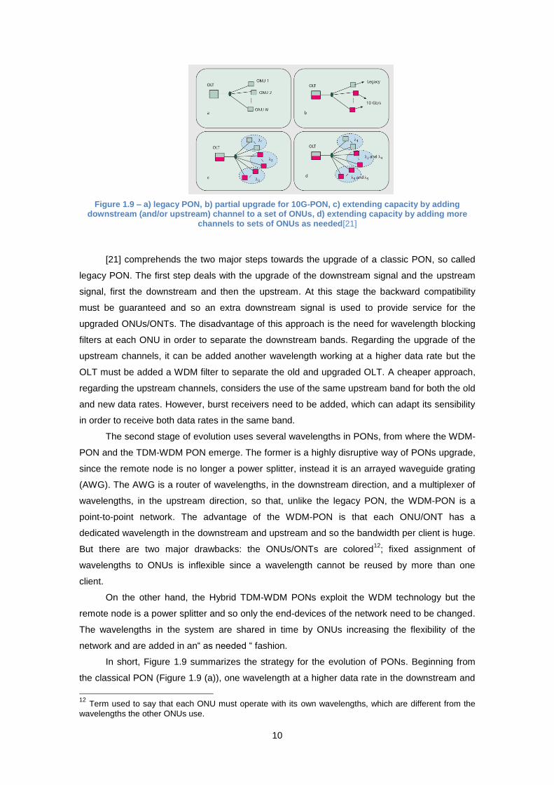
Figure 1.9 – a) legacy PON, b) partial upgrade for 10G-PON, c) extending capacity by adding downstream (and/or upstream) channel to a set of ONUs, d) extending capacity by adding more
channels to sets of ONUs as needed[21]
[21] comprehends the two major steps towards the upgrade of a classic PON, so called
legacy PON. The first step deals with the upgrade of the downstream signal and the upstream
signal, first the downstream and then the upstream. At this stage the backward compatibility
must be guaranteed and so an extra downstream signal is used to provide service for the
upgraded ONUs/ONTs. The disadvantage of this approach is the need for wavelength blocking
filters at each ONU in order to separate the downstream bands. Regarding the upgrade of the
upstream channels, it can be added another wavelength working at a higher data rate but the
OLT must be added a WDM filter to separate the old and upgraded OLT. A cheaper approach,
regarding the upstream channels, considers the use of the same upstream band for both the old
and new data rates. However, burst receivers need to be added, which can adapt its sensibility
in order to receive both data rates in the same band.
The second stage of evolution uses several wavelengths in PONs, from where the WDM-
PON and the TDM-WDM PON emerge. The former is a highly disruptive way of PONs upgrade,
since the remote node is no longer a power splitter, instead it is an arrayed waveguide grating
(AWG). The AWG is a router of wavelengths, in the downstream direction, and a multiplexer of
wavelengths, in the upstream direction, so that, unlike the legacy PON, the WDM-PON is a
point-to-point network. The advantage of the WDM-PON is that each ONU/ONT has a
dedicated wavelength in the downstream and upstream and so the bandwidth per client is huge.
But there are two major drawbacks: the ONUs/ONTs are colored12
; fixed assignment of
wavelengths to ONUs is inflexible since a wavelength cannot be reused by more than one
client.
On the other hand, the Hybrid TDM-WDM PONs exploit the WDM technology but the
remote node is a power splitter and so only the end-devices of the network need to be changed.
The wavelengths in the system are shared in time by ONUs increasing the flexibility of the
network and are added in an“ as needed “ fashion.
In short, Figure 1.9 summarizes the strategy for the evolution of PONs. Beginning from
the classical PON (Figure 1.9 (a)), one wavelength at a higher data rate in the downstream and
12
Term used to say that each ONU must operate with its own wavelengths, which are different from the
wavelengths the other ONUs use.

11
then in the upstream (Figure 1.9 (b)) is added. The next step is to increase the number of
wavelengths so to reduce the number of ONUs sharing the same wavelength, creating several
groups of ONUs (Figure 1.9 (c)).Finally, each group of ONUs is given extra wavelengths in an
“as needed “ fashion (Figure 1.9 (d)). The evolution process presented in Figure 1.9 has two
fundamental properties, which are the backward compatibility with the classical PON, and
flexibility regarding the wavelength assignment.
In the context of access networks, [22] used the integer linear programming (ILP)
formulations to simulate several network paradigms with many restrictions. The purpose of its
author was to study the PON planning strategies, for single-staged PONs or multi-staged PONs,
taking into account the restrictions each PON system has.
In spite of addressing different problems related with optical access networks, the work of
this thesis and the one of [22] share the same ultimate goal of searching for the least expensive
network paradigm. Therefore, the work presented in [22] was crucial to understand how the
network planning and ILP formulation meet together.
Reference [23] shows an interesting upgrade of the upstream channels for GPONs taking
advantage of the temperature dependent transmission characteristic of the lasers. The variation
of the transmitter wavelength with the temperature is exploited to divide the GPON receiver
band - Figure 1.8 - in four sub-sections. So, clients would be divided into four types/groups and
their ONUs would be thermally conditioned to match a specific sub-band within four possible.
Each group would then have at its disposal 2.5 Gbps to share among the ONUs of the same
group, paradigm that promises an overall total upstream data rate of 10 Gbps, with minor
changes at the ONUs.
[24]take the upgrade investigation to a next level, considering an Hybrid TDM/WDM PON
that provides an “as needed“ fashion of upgrading the clients, taking into account their needs
and a pricing policy. The main goal of such paper is to create several paradigms of evolution for
hybrid TDM/WDM PONs at the level of the ONUs by using different types of devices, namely
single wavelengths transceivers or groups of transceivers.
The conditions of this paper will be further explained and investigated in the second
chapter because it was decided as the starting point for this thesis.
A more futurist approach for the upgrade of PONs is detailed in [25]. It considered the
use of AWGs in both the central office and remote node of the network with the purpose of
wavelength allocation inflexibility mitigation inherent in the WDM-PON.
1.4. Motivation, Objectives and Structure
Given the importance of upgrading the passive optical networks aiming its match with the
customers´ expectations in the future, and the constraints that arise by doing that represent the
main motivation for this thesis. Furthermore, the study concerns the upstream channels since

12
they are the bottleneck of PONs, being shared using the time division multiple access technique
(TDMA).
Some internet services nowadays are evolving to go distributed, rather than centralized.
The end-user is gaining an importance, never seen before, regarding the generation of
information, whether it is audio, video or text, bringing alive an urgent need for symmetric
communication between the end user and the network itself.
The objective is to develop some ILP models that capture the picture of the passive
optical network in the near future, aiming to do some paradigms about those networks and
compare the results.
The thesis is structured as follows:
The first chapter presents the passive optical networks details, PON implementations that
are already massively deployed, as well as the already standardized next generation passive
optical networks.
The second chapter studies the Hybrid TDM/WDM PON as a first network suitable for
short-term evolution of current PONs. The ILP presented in [24] is analyzed and its scope is
extended, in terms of the number of ONUs in the network, to understand the cost of the
upgrade.
Chapter 3 is where the first two original ILP models are presented, their results are shown
and compared, regarding the hybrid TDM/WDM PON, which used tunable lasers at the ONUs
and the CWDM grid.
The chapter 4 is where an extra variable is added to the first model presented in the
Chapter 3. As a results, that model is capable of simulate the hybrid TDM/WDM PON with
tunable lasers and receivers working at 10 Gbps or 40 Gbps.
In chapter 5 another original ILP model is shown and explained, this time exploiting the
cyclic propriety of the AWGs to reach another type of passive optical network whose channels
can be upgraded in an “as needed“ fashion from a DWDM grid.
Finally, chapter 6 contains the overall conclusion plus my proposal for a future work
related with the study theme of this thesis.
1.5. Original Contributions
From the five ILP models presented in this document, four are original. Two of them were
built aiming a PON system using tunable lasers at the client side, in such a way, that was not
found during the course of this thesis. The model where the 40 Gbps channels are introduced
have not yet been studied the way presented here and the same happens with the fourth model
that includes the AWG in the access network.

13
2. Migration Scenario to the Next
Generation PON
In this chapter, the Hybrid TDM-WDM PON is going to be analyzed based on the
reference [24], “Optimizing the Migration to Future-Generation Passive Optical Networks
(PONs)”, widely invoked. Firstly, its ILP formulation will be presented and understood as well as
its pricing policy (that regards single wavelength transceivers). Secondly, one of the several
modes of simulation presented in that paper, called 1x1Tx, is going to be confirmed. Finally, the
extend the scope of [24] by simulating the network with 32 and 64 ONUs, using the 1xTx mode,
in order to understand the behavior of the cost.
,

14
2.1. Description of the paradigm
Hybrid TDM/WDM PON presents some features suitable for the next generation passive
optical networks and the paper “Optimizing the Migration to Future-Generation Passive Optical
Networks (PONs)” [24] formulates an evolution paradigm based on that network worth to be
explained.
OLT
Po
wer
Splitter
1
2
3
4
5
6
7
8
9
10
11
12
13
14
15
16
ONU 7
ONU 14
ONU 15
ONU 8
Group 1 using λ1 and λ
2
time
time
time
time
λ2 λ3 λ4 λ5 λ6 λ7 λ8 λ1
Grid of wavelengths for the upstreamGroup 2 using λ
3 and λ4
Group 3
usin
g λ5 a
nd λ 6
Group 4
usin
g λ7 a
nd λ 8
Figure 2.1 - Hybrid TDM/WDM PON (upstream perspective)
An hybrid TDM-WDM PON (Figure 2.1) is a network that uses both TDM and WDM
techniques. Both upstream and downstream have a grid of wavelengths whose channel spacing
depends on the WDM technology (CWDM13
, DWDM or something else) in question. This way,
several wavelengths flow in the network (WDM principle). Still, the number of wavelengths in
each direction is most likely to be fewer than the number of ONUs, so there are groups of ONUs
which share one or several wavelengths in time (TDM principle). The dynamic bandwidth
allocated in the OLT will need to assign not only time-slots to ONUs, but also wavelengths.
Therefore, before transmitting, an ONU needs to know the wavelength and time-slot that is
going to use. For ONUs belonging to the same groups, the time-slots cannot overlap in time if
the transmission is done using the same wavelengths, whereas for ONUs of different groups the
transmission is independent.
13
CWDM uses a channel spacing of 20 nm

15
Unlike what happens in a WDM-PON, the remote node is not changed, remaining a
power splitter. Consequently, ONUs need to be added wavelength blocking filters, which leave
all the possible upstream wavelengths pass as well as the downstream wavelengths assigned
to the ONU in question and block all the other wavelengths.
Adding the bonus of having no need for remote node substitution, the hybrid TDM-WDM
PON keeps exploring the statistical multiplexing of channels in the same way as in classical
PONs, which is an important feature for networks that carry bursty traffic. If a group of ONUs,
containing four ONUs, share a 1 Gbps wavelength, it is expected that each ONU can use 250
Mbps. Still, if in a given moment, one or more ONUs are using less than 250 Mbps and another
ONU needs to use more than 250 Mbps, there is no problem, as long as the total capacity of the
wavelength channel is not exceeded.
Figure 2.1 shows the hybrid TDM-WDM PON architecture with sixteen ONUs, which
contain four groups of ONUs sharing two wavelengths each. That figure presents the
perspective of the upstream and the transmitting paradigm is shown in the left bottom image of
that figure.
Given the sustained traffic grow, it is expected that emerging applications will exceed
today´s access network capacity, and so PONs will need line-rate upgrades and/or additional
wavelength channels.
As previously mentioned, [24] starts from the paradigm of a single wavelength per
direction and moves toward an Hybrid TDM/WDM PON (as the demand by customers
increase), where only the end devices of the network need to be upgraded. However, one of the
golden rules for upgrading an existing network is never waste the previous resources, which in
a hybrid TDM/WDM PON are the transceivers (end devices of the network).
As the new wavelengths channels (that can work at 10 Gbps or 40 Gbps) are added in
the PON, consequence of the increase of bandwidth per client, it is crucial to figure out who are
the clients that actually need an upgrade in its end device that need to increase its number of
transceivers), so to minimize the upgrading cost. To accomplish that, [24] uses a multistep cost-
and-network-upgrade model based on Mixed Integer Linear Programing (MILP) formulations
and pricing policies.
A MILP is a formulation used to determine the minimum or maximum of a certain function,
called objective function, containing variables. Such function is a linear one because its
variables are only allowed to have constant coefficients. The number of variables in the
objective function defines the dimensions of the MILP. The domain of the variables is defined in
the problem according to the needs and there are integer variables and float variables in the
problem, which is why it is called Mixed. Besides the objective function, the MILP has several
constraints the programmer needs to set in order to account for the restriction of the problem in
question.
The pricing policies are used to build the objective function, more precisely it decides how
valuable is a certain constant that multiplies for a variable. In the context of this Hybrid TDM-

16
WDM PON, the pricing policy determines the cost of using a new wavelength channel in the
OLT and ONUs. Such cost depends on the data rate of the transceivers.
2.2. MILP formulation
Regarding the problem explained in the last section, [24] uses the following MILP formulation
Variables:
binary variable that is 1 if the ith ONU is operating on wavelength j with rate k; note
that an ONU, in order to support an additional wavelength j, needs to be equipped with
an additional transceiver;
binary variable that is 1 if the jth wavelength is operative on rate k;
binary variable that is 1 if the ith ONU has any traffic over wavelength j;
integer variable that represents the maximum bandwidth occupation over all
wavelengths.
Constants:
K set of line rates supported by the PON ;
N set of ONUs existing in the PON;
L set of wavelengths that can be used in the PON;
cost per unit of bandwidth to support load balancing over all wavelengths ;
value in Mbps of the kth line rate;
value used to obtain a binary number out of an integer, and accomplishes :
maximum number of wavelength channels that ONU i can support.
Constants for Multiple Periods: The following constants will change with every period in which
we apply the MILP, in order to calculate how a PON evolves. These constants will link one
period to the other
cost to support wavelength j with rate k at the OLT;
cost to support wavelength j with rate k at the ONU i;
previous line-rate value of jth wavelengths before running the MILP;
guaranteed bandwidth for ONU I;
set of wavelengths that have not been allocated to ONU i in any previous step
number of wavelength channels previously supported by ONU i.

17
Objective Function :
Subject to :
Equation (1.1) is a triple-objective function. The first and second terms stand for the cost
of supporting wavelength j with line rate k at the ONUs and at the OLT, respectively. Here, cost
is the cost per added transceiver. The third term represents the maximum utilization among all
wavelengths with lower priority (given by a small value α). Thus, our objective is to minimize the
cost of supporting a new wavelength at a given line rate by the ONUs, minimize the cost of

18
supporting a new wavelength at a given rate by the OLT, and, with a small priority, minimize the
maximum use among all wavelengths in the PON (which performs load balancing, where load is
fractional capacity use). The cost here is associated to capital expenses to install transceivers
at OLT and ONUs. Equation (1.2) constrains the maximum amount of traffic that can be placed
on each wavelength. Equation (1.3) restricts the possible line rate that a wavelength channel
can take according to the value of the previous line rate: according to Equation (1.3), a
wavelength channel’s line rate can only increase or remain the same. Equation (1.4) ensures
that the bandwidth assigned to an ONU satisfies its guaranteed bandwidth requirements.
By using Equation (1.5) and Equation (1.6), we associate a binary variable to the
integer variable introducing a “big M” inequality. Equation (1.7) limits the number of channels
that an ONU can use to support the traffic (note that second term of Equation (1.7) accounts for
both the number of existing transceivers and the newly enabled transceivers ). Equations
Equation (1.8) and Equation (1.9) discard the possibility of having two different line rates over
the same wavelength.
There is a logical relation among all the binary variables , and enforced in
Equation (1.10), which implies that ONU i can only operate over wavelength j with rate k if that
wavelength has rate k, and that ONU has traffic flowing over wavelength j. Finally, in (1.11),
variable takes the value of maximum traffic occupation among all wavelength channels.
2.3. Multiple period simulation
The ILP runs under a several period simulation, whose duration is determined by the
programmer, and from period to period the network demands more traffic than in the previous
periods, by a factor determined as an entry parameter of the simulation.
Forecast the Traffic for the period t
t>1
Start
Collect Historical Data from the
period t-1
Apply Pricing Policies for the
Period t
Run MILP
Output the results for the period t
Are the perods over?
End
t=t+1
Yes
No
Yes
No
Figure 2.2 – Simulation´s flowchart
All periods of the simulation are connected between each other, like a TV stream. So,
what happens in the period t is influencing the following periods until the end of the simulation

19
as Figure 2.2 is showing. The duration of each period is not defined and is up to the service
provider to determine it, according with its study intentions. Therefore, it is defined as the
duration clients take to increase its bandwidth demand by a certain value (determined as an
entry value of the simulation).
In a superficial snapshot, the simulation begins - Figure 2.2 - by forecasting the
bandwidth needed for every client in the PON. Then, if the period is not the initial one, the
results from the last MILP simulation are scanned, in a procedure called “Collect Historical
Data“. Here, the program looks for wavelengths that were allocated to the PON system, through
the , and searches for the wavelengths each ONU is using, through the . Moving on, the
simulation will then enter the “ Appling pricing policies“ sub-routine and uses the information
taken from the “ Collect Historical Data“ to adjust the costs according with the status of each
wavelength in the PON, and the wavelengths each ONU was already using before a certain
period of the simulation. Finally, the information of “Appling pricing policies” will be used to build
the objective function of the MILP and the information taken from “Collect Historical Data“ is
gathered to upgrade the constraints of the MILP. At last, the MILP is executed. After that, if the
number of simulation periods is over the simulation ends, otherwise the cycle of routines is done
again, starting from the “forecast the bandwidth“ sub-routine.
2.4. Results and discussion
This section presents some results to illustrate the application of the methodologies
described and to confirm the results presented in [24]. In this way, a C++ program has been
developed, which relies on the CPLEX framework to solve the MILP problem and runs on an
Intel Core2 Duo at 2,33 GHz processor with 2 GB of memory.
The MILP presented in this section can be used to study either the downstream or upstream
channels, but following what was done in [24] only the upstream channels will be considered.
The simulation has 16 ONUs, belonging to two different types, the first type, 6 ONUs, can only
support one wavelength channel during the whole simulation ( ) and the second type, 10 ONUs,
can support up to four ( ). At the beginning of the simulation there is only one wavelength
working at 10 Gbps in the PON, serving the upstream, and the first type of ONUs start with 100 Mbps
(so ) each, whereas the second type start with 600 Mbps (so ) each (Note: All
ONUs, regardless of the type, have already allocated one transceiver working at 10 Gbps, whose
cost does not entry the MILP). The wavelength channels can work at 10 Gbps or 40 Gbps (so
and ). The total number of periods of the simulation is six and from period
to period the traffic demand increases by 50 percent.
[24] presents the reader with three different pricing policies but only the single wavelength
transceiver policy, so called 1xTx, is going to be considered here. As its name suggests, such pricing
policy guarantees that when an ONU needs extra transceivers it will be given one single wavelength
transceiver at a time and the objective function will account for that. The costs of the pricing policy
have a relative nature whose reference equipment is the 10 Gbps single wavelength transceiver.

20
A pricing policy determines the value of and taking into account the presence (or
not) of the wavelengths in the PON as follows. To calculate for a given period three cases
must be analyzed : (i) if the previous line rate of wavelength j is zero (wavelength channel that
has not been deployed yet), then and to activate wavelength j for the first
time, (ii) if wavelength j was active at line rate , then and (higher value than
in (ii) to reflect the line-rate change), (iii) if wavelength j was active at line rate , then
(extreme high value because downgrades are not allowed) and . Now to calculate
, information from the OLT and the ONU i is needed. If the ONU i was already supporting
the wavelength j, then , otherwise .
In the simulations where the number of ONUs was changed from 16 to 32 and 64,
everything was left the same, except for the number of ONUs each type has and their
respective initial bandwidth ( ). For 32 ONUs, 8 ONUs are type one with and
24 ONUs are type two with . Whereas for 64 ONUs, 12 ONUs are type one using
an initial bandwidth of 55 Mbps each, and 52 ONUs are type two using an initial bandwidth of 114,2
Mbps. Note that for all the setups presented, the total initial bandwidth for the ONUs is the same (6,6
Gbps).
2.4.1. Results
Two level of results will be shown here. Firstly, the wavelengths allocation pattern per
ONU and period, followed by the resulting channel occupation per period (For the setup of
simulation with 16 ONUs). Then, the information that drives the cost of upgrading the network is
presented for the simulations with 16, 32 and 64 ONUs.
Period 1 Period 2 Period 3 Period 4 Period 5 Period 6
ONU 1 [900]λ1 [1350]λ1 [2025]λ3 [3038]λ3 [4557]λ4 [3165]λ3, [3670]λ4
ONU 2 [900]λ1 [1350]λ1 [2025]λ3 [3038]λ3 [4557]λ3 [6835]λ4
ONU 3 [900]λ1 [1350]λ2 [2025]λ2 [3038]λ1 [4557]λ2 [6835]λ2
ONU 4 [900]λ1 [1350]λ1 [2025]λ1 [3038]λ1 [4557]λ1 [6835]λ2
ONU 5 [900]λ1 [1350]λ1 [2025]λ1 [3038]λ3 [4557]λ3 [6835]λ5
ONU 6 [900]λ1 [1350]λ2 [2025]λ2 [3038]λ2 [4557]λ2 [6835]λ2
ONU 7 [900]λ1 [1350]λ2 [1011]λ1, [1014]λ2
[3038]λ2 [4557]λ2 [6835]λ2
ONU 8 [900]λ1 [1350]λ1 [2025]λ2 [3038]λ2 [4557]λ2 [6835]λ2
ONU 9 [900]λ1 [1350]λ1 [2025]λ1 [3038]λ4 [4557]λ4 [505]λ1, [6330]λ4
ONU 10 [900]λ1 [1350]λ2 [2025]λ2 [3038]λ4 [4557]λ2 [2655]λ1, [4180]λ2
ONU 11 to ONU 16
[150]λ1 [225]λ1 [338]λ1 [507]λ1 [760]λ1 [1140]λ1
Table 2.1 – wavelength allocation per ONU and period for the 1xTx mode and 16 ONUs (Notation [x Mbps]λi, x upstream traffic demand by ONU i ; the bold text represents a new wavelength at 10 Gbps in the ONU i, blue text represents wavelengths at 40 Gbps in the ONU i, and bold blue text
gathers the information of the blue and bold text already explained)
21
In the simulation with 16 ONUs - Table 2.1 - five wavelengths are needed in total, and
one of them is working at 40 Gbps. The initial channel, channel #1(λ1) can support the traffic for
one period but from there on a new wavelength channel (in period 2, 3, 4, 5 and 6) needs to be
added, or the line rate of an existing wavelength is upgraded from 10 Gbps to 40 Gbps (in
period 5). The ONUs 11 to 16 only use the channel #1 because only one transceiver can be
assigned to them. The remaining ONUs could have up to four transceivers, but that value is not
achieved. In fact, ONU 1, 3, 4, 6, 7, 8 and 9 support two wavelength channels and ONU 2, 5
and 10 support three wavelength channels, including the initial channel, λ1. In several periods,
ONUs may need to use more than one wavelength in the same period, as seen for ONU 7 in
period 3, for example, showing that this feature is important to increase the degree of
smoothness during the upgrade of the network. Regarding the ONU number seven, it uses two
lasers to transmit at the period 3 because the alternative would be the introduction of another
transceiver to transmit over the wavelength channel #3 (λ3), increasing the cost of the upgrade
by one unit at the period in question.
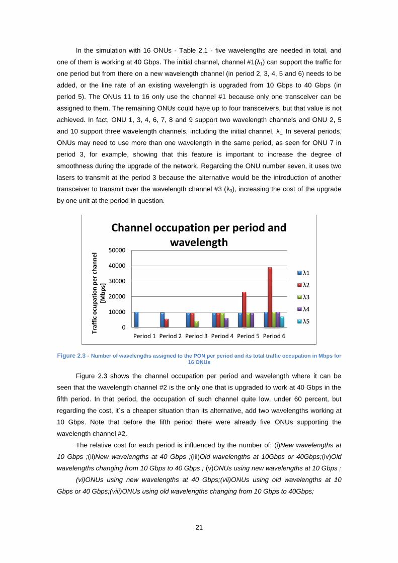
Figure 2.3 - Number of wavelengths assigned to the PON per period and its total traffic occupation in Mbps for
16 ONUs
Figure 2.3 shows the channel occupation per period and wavelength where it can be
seen that the wavelength channel #2 is the only one that is upgraded to work at 40 Gbps in the
fifth period. In that period, the occupation of such channel quite low, under 60 percent, but
regarding the cost, it´s a cheaper situation than its alternative, add two wavelengths working at
10 Gbps. Note that before the fifth period there were already five ONUs supporting the
wavelength channel #2.
The relative cost for each period is influenced by the number of: (i)New wavelengths at
10 Gbps ;(ii)New wavelengths at 40 Gbps ;(iii)Old wavelengths at 10Gbps or 40Gbps;(iv)Old
wavelengths changing from 10 Gbps to 40 Gbps ; (v)ONUs using new wavelengths at 10 Gbps ;
(vi)ONUs using new wavelengths at 40 Gbps;(vii)ONUs using old wavelengths at 10
Gbps or 40 Gbps;(viii)ONUs using old wavelengths changing from 10 Gbps to 40Gbps;
0
10000
20000
30000
40000
50000
Period 1 Period 2 Period 3 Period 4 Period 5 Period 6
Traf
fic
ocu
pat
ion
pe
r ch
ann
el
[Mb
ps]
Channel occupation per period and wavelength
λ1
λ2
λ3
λ4
λ5
22
The first four topics represent the cost at the OLT side, mapped by the , whereas the
rest represent the cost at the ONUs side, mapped by the The total relative cost for a certain
period is the sum of for all the wavelengths that are working in the PON plus the sum
of for all the ONUs of the PON system.
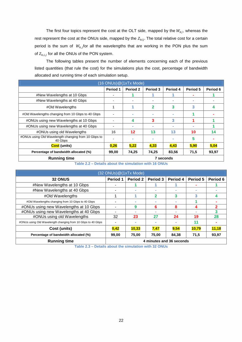
The following tables present the number of elements concerning each of the previous
listed quantities (that rule the cost) for the simulations plus the cost, percentage of bandwidth
allocated and running time of each simulation setup.
(16 ONUs)@(1xTx Mode)
Period 1 Period 2 Period 3 Period 4 Period 5 Period 6
#New Wavelengths at 10 Gbps - 1 1 1 - 1
#New Wavelengths at 40 Gbps - - - - - -
#Old Wavelengths 1 1 2 3 3 4
#Old Wavelengths changing from 10 Gbps to 40 Gbps - - - - 1 -
#ONUs using new Wavelengths at 10 Gbps - 4 3 3 1 1
#ONUs using new Wavelengths at 40 Gbps - - - - - 1
#ONUs using old Wavelengths 16 12 13 13 10 14 #ONUs using Old Wavelength changing from 10 Gbps to
40 Gbps - - - - 5 -
Cost (units) 0,26 5,22 4,33 4,43 5,90 5,04
Percentage of bandwidth allocated (%) 99,00 74,25 74,25 83,56 71,5 93,97
Running time 7 seconds
Table 2.2 – Details about the simulation with 16 ONUs
(32 ONUs)@(1xTx Mode)
32 ONUS Period 1 Period 2 Period 3 Period 4 Period 5 Period 6
#New Wavelengths at 10 Gbps - 1 1 1 - 1
#New Wavelengths at 40 Gbps - - - - - -
#Old Wavelengths 1 1 2 3 3 4
#Old Wavelengths changing from 10 Gbps to 40 Gbps - - - - 1 -
#ONUs using new Wavelengths at 10 Gbps - 9 6 8 4 2
#ONUs using new Wavelengths at 40 Gbps - - - - - 3
#ONUs using old Wavelengths 32 23 27 24 19 28
#ONUs using Old Wavelength changing from 10 Gbps to 40 Gbps - - - - 11 -
Cost (units) 0,42 10,33 7,47 9,54 10,79 11,18
Percentage of bandwidth allocated (%) 99,00 75,00 75,00 84,38 71,5 93,97
Running time 4 minutes and 36 seconds
Table 2.3 – Details about the simulation with 32 ONUs

23
(64 ONUs)@(1xTx Mode)
64 ONUS Period 1 Period 2 Period 3 Period 4 Period 5 Period 6
#New Wavelengths at 10 Gbps - 1 1 1 - 1
#New Wavelengths at 40 Gbps - - - - - -
#Old Wavelengths 1 1 2 3 3 4
#Old Wavelengths changing from 10 Gbps to 40 Gbps - - - - 1 -
#ONUs using new Wavelengths at 10 Gbps - 20 12 18 6 5
#ONUs using new Wavelengths at 40 Gbps - - - - - 4
#ONUs using old Wavelengths at 10 Gbps 64 44 52 48 34 55
#ONUs using Old Wavelength changing from 10 Gbps to 40 Gbps - - - - 24 -
Cost 0,74 21,54 13,72 19,78 16,84 16,95
Percentage of bandwidth allocated (%) 99,00 75,00 75,00 84,38 71,5 93,97
Running time 1 hour and 36 minutes
Table 2.4 – Details about the simulation with 64 ONUs
As the number of ONUs in the PON increase, the total number of wavelength channels
needed doesn´t increase and the way they are introduced and upgraded remains the same (see
the first four rows of Table 2.2, Table 2.3, Table 2.4), since the initial bandwidth was set to be
the same for the simulations with 16, 32 and 64 ONUs. Moreover, the percentage of bandwidth
allocated pattern does not change unlike the running time that increases dramatically.
Number Of ONUs
Cost(units)
16 25,18
32 49,73
64 89,57 Table 2.5 – Total Cost for 16, 32 and 64 ONUs in the PON
As the number of ONUs change, the period when the cost is higher in the simulation,
apart from the period 1, change as well. In the setup with 16 ONUs, the higher value of cost
happens at the fifth period, but for 32 ONUs and 64 ONUs such maximum moves to the sixth
period and second period, respectively.
According to the simulations of 16 ONUs and 32 ONUs, the simulation of 64 ONUs was
expected to cost around 100 units of cost (when applying a linear rule). However, its total cost is
well below that - Table 2.5 - by around 10 units of cost, due to the lower cost of the fifth and
sixth periods.
2.5. Conclusion
Comparing the results of this chapter with those from [24], some differences have been
noticed, which will be further explained and justified.

24
Figure 2.5 – the same information given by Table 2.1 but directly from [24]
The wavelength allocation per ONU and period, until the fifth period, taken from the
program developed for the thesis and its counterpart from [24] have the same behavior (by
comparing Figure 2.5 and Table 2.1). This means the number of wavelengths added until such
period are the same and so is the number of ONUs that were upgraded. Note that at the second
period, ONUs that were upgraded to support the wavelength channel #2 are not exactly the
same in both simulations (ONU 5, 7, 8 and 9 for the simulation of the paper and 3, 6 7 and 10
for the simulation of the thesis). But that fact does not matter because ONUs from 1 to 10 have
exactly the same characteristics in terms of initial bandwidth and traffic growth factor. Still,
ONUs receiving the wavelength channel #2 at the second period will influence the following
period, because wavelength continuity is assured by the MILP as long as possible. For
example, in Figure 2.5 (results of the paper), at the third period, ONU 10 is given one
transceiver to use the wavelength channel #3; now going back to Table 2.1 (results from the
thesis), for the same period and ONU no transceiver is added because such ONU had already
two transceivers at its disposal (one for the wavelength channel # 1 and another for the
wavelength #channel #2), and was one of the ONUs that was given the access for the
wavelength channel #2 at the second period.
And so, this is the reason why, even until the fifth period, the results in question may look
different but, in fact, are equivalent. Until that period, the important information for the PON
evolution is the number of wavelength channels added (one for period) and the number of
ONUs receiving new transceivers (four in the second period and three in the third and fourth
periods), which are exactly the same for both simulations.
In the fifth period, no new transceiver was expected to be allocated to any ONU,
according with the results from the paper (Figure 2.5). However the simulation done for the
thesis decided to add a new transceiver in the ONU 1, which increased the total cost of upgrade
by about one unit of cost. Given the fact that the channel #3 and #1 (channels supported by the
Figure 2.4 - Same information given by Figure 2.3
but taken directly from [24]

25
ONU 1) were almost full, the only two options the MILP had regarding the ONU 1 was to
allocate one transceiver for the wavelength channel #4 or #2. In the end, the channel #4 was
chosen because the channel #2 was being upgraded from 10 Gbps to 40 Gbps and its
transceivers would cost three times more than the transceiver for the channel #4. Finally, at the
fifth period, both simulations concord again.
Regarding the traffic occupation per channel and period, both simulations match
completely, as the Figure 2.3 and 2.4 shows.

26
3. Migration scenario reformulated
In this chapter, the study of hybrid TDM/WDM PONs is continued by introducing tunable
lasers in the ONUs and a specific ITU wavelength grid to serve the upstream, the CWDM grid.
In this paradigm two modes are studied and analyzed. For each mode, several setups are going
to be considered, by varying the range of tunable lasers and the number of ONUs (16, 32 and
64 ONUs).
Finally, the results for the two modes are presented and discussed aiming to understand
if there is any real difference, in terms of costs, between the models.

27
3.1. Wavelength grids
The model studied in the previous chapter has some issues when we try to apply it to the
real world. The number of wavelengths that can be allocated to the PON system, theoretically,
are infinite, which is not a good starting point if we want to study a real scenario of evolution for
the passive optical networks and this stands as its first drawback.
Before mass deployment, a certain optical technology needs to be standardized by a
certain SDO, like the ITU or IEEE. The access network technologies have been fitting this
procedure. Study the number of wavelength channels in the network is one of the critical task of
such procedure. For that purpose, ITU-T standardized two grids, the dense wavelength-division
multiplexing (DWDM) and course wavelength-division multiplexing (CWDM) grid.
DWDM and CWDM are two technologies that can provide the transportation of several
wavelengths using one single fiber, but have many differences between them. The DWDM only
works in C and L band and each channel has a variable size (but the most common grid has a
channel spacing of 50 GHz), whereas the CWDM covers the O, E, S, C and L band using a
channel spacing of 20 nm. The DWDM is capable of transmitting over longer distances than the
CWDM because it uses the Erbium-Doped Fiber Amplifier, whereas the CWDM does not. The
number of channels provided by the DWDM can be 40, 80 or even more, unlike the CWDM,
which uses only 17 or 18 channels.
The channel spacing determines how far the laser wavelength can drift from the nominal
wavelength. The shorter the channel spacing, the shorter can be the drift. To better control the
drift, coolers must be added to the laser which results in a bigger and more energy demanding
device.
In fact, the DWDM laser occupies eight times the space of the CWDM laser and it
consumes about twenty times more power than a CWDM laser. Because of this, the DWDM
laser exceeds the price of its CWDM counterpart by four or five times.
Regarding the receiver, the CWDM and DWDM use the same type of receivers that can
be a wavelength agnostic PIN or an avalanche photodiode detector. The latter is more
expensive, but is more sensitive as well, resulting in a gain of 9 to 10 dB in the power budget.
The filters for the CWDM and DWDM are made using the thin-film filter (TFF) technology.
These filters can appear as a discrete single-channel filter devices or as an integrated
multiplexer/ demultiplexer. CWDM filters are inherently less expensive to make than DWDM
filters due to the fewer layers in the filter design.
Taking into account the facts mentioned above, CWDM has the cheapest implementation
for. It has been available since the 1990s on property telecommunications systems, but its mass
deployment happened after 2002, year of its standardization by the ITU-T. Although it is being
used already at the access level of the network, its usage is just for specific clients, not for the
entire fiber access clients.
In this chapter and in the following one, the hybrid TDM/WDM PON uses a CWDM grid in
order to be able to suffer mass deployment and compatibility between different manufactures of

28
the equipment. The CWDM grid is going to be splitted into two areas as Table 3.1 shows. The
upstream channels are represented in blue spots, and the downstream channels are
represented in green spots.
Nominal central wavelengths [in nm] for spacing of 20 nm
1271 1291 1311 1331 1351 1371 1391 1411 1431 1451 1471 1491 1511 1531 1551 1571 1591
Table 3.1 – ITU-T G694.2 CWDM grid
Although there are nine upstream channels, only eight are going to be considered
because the 1271 nm is reserved for the legacy wavelength (wavelength coming from the single
wavelength PON that is predecessor of the Hybrid TDM/WDM PON in the evolution path).
3.2. Reformulating the upgrade scenario
Using single wavelength transceivers at the ONUs, in the way done in the previous
chapter, is an inflexible way of upgrading the network because the more transceivers an ONU
needs (it was seen in the last chapter that certain ONUs may need one or two transceivers
beyond the initial transceiver), the higher will be the operational expenditures (OPEX) related
with the substitution of clients´ equipment.
To increase the flexibility of the network, tunable lasers can be used [21] inside the
upstream band of the CWDM grid. There are tunable lasers[26] capable of sintonize the entire
CWDM band but their cost is overwhelming, discarding their use at the access level. Still,
maybe in a few years’ time this type of tunable lasers, or at least some other type that sintonize
part of the CWDM, can be at the price level of the access network. Tunable lasers have a
continuous tuning range, but the paradigms formulated here will need discrete values for the
wavelengths, more precisely, for each 20 nm of band only one specific wavelength will be used
(the one at the center). The reason for this lies in the fact that it is considered to use CWDM
compliant receivers at the OLT.
Regarding the tunable lasers, two different models are going to be simulated and
compared. Each simulation setup will use exclusively one type of tunable laser. This means that
if the simulation has tunable lasers of two wavelengths, then the entire ONUs will be tested with
lasers of such type.

29
Laser 1 (p=1)
Laser 2 (p=2)
Laser 3(p=3)
Laser 4(p=4)
Laser 1 (p=1)
Laser 2 (p=2)
Laser 1 (p=1)
λ1 λ2 λ3 λ4 λ5 λ6 λ7 λ8 λ9
Laser 0 (p=0)
Laser 0 (p=0)
Laser 0 (p=0)
Figure 3.1 - Distribution of the wavelengths per lasers, using lasers of two, four and eight wavelengths (Model One)
Concerning the first model, each laser has its own wavelengths and does not overlap with
the wavelengths of the other lasers, as Figure 3.1 shows. The wavelength number one, in blue,
is the legacy wavelength. Nevertheless, different ONUs can use lasers that transmit the same
wavelengths at the same time. Figure 3.2 shows several setups, one per row, with different
wavelengths per laser. In the first row, four lasers are needed to fill the entire CWDM band and
the ONUs will be given one of them if needed. Note that one ONU with Laser 1, can be given
another Laser 1 in order to transmit both wavelengths that such laser can transmit, wavelength
#1 and #2, simultaneously.
Laser 1 (p=1)
Laser 3 (p=3)
Laser 2 (p=2)
λ1 λ2 λ3 λ4 λ5 λ6 λ7 λ8 λ9
Laser 0 (p=0)
Figure 3.2 - Number of laser types, five (but only 3 are represented in the figure), for eigth wavelength channels and four wavelengths per laser (Second Model)
Regarding the model two, tunable lasers used may share wavelengths with other tunable
lasers. In Figure 3.2, for example, Laser 1 shares wavelength #2,#3 and #4 with the Laser 2.
The same way Laser 2 shares wavelength number 4,5 and 6 with Laser 3.
Given the total number of wavelengths available in the system [N] and the number of
wavelengths a laser can tune [ ], where , the total number of different lasers that can be
used is set by the next formula : .
Note that in both models, there is a pre-allocated wavelength, wavelength channel #1 (in
blue in the Figure 3.1 and Figure 3.2).

30
3.3. MILP models
In this section the two MILP models of this chapter will be presented and analyzed.
3.3.1. Model One
This model corresponds to the situation where the lasers used are allocated in the
CWDM band the way Figure 3.1 is showing.
Variables:
integer variable with the maximum value of bandwidth load among all the
wavelengths belonging to the same group, where p is the index of that group. The
wavelengths of the same group can be transmitted by the same tunable laser.
integer variable that represents the bandwidth in the j wavelength of the p group
demanded by the ONU i ;
binary variable that is 1 if the j wavelength of the p group is available in the PON
system;
binary variable that is 1 if the ONU i wants to use the wavelength j of the p tunable
lasers ;
binary variable that is one if the ONU i has traffic over the j wavelength of the p
tunable laser.
Constants:
number of wavelengths the p tunable laser has.
number of ONUs in the PON.
set with the groups of wavelengths/different tunable lasers that can be used.
cost to support the wavelength j of the p tunable laser by the ONU number i.
cost to support the j wavelength belonging to the p tunable laser at the OLT side
cost per unit of bandwidth to support load balancing over all wavelengths.
is the only data rate available in the model.
is the total bandwidth required by the ONU number i.
Objective Function:

31
Subject to:
The objective function has three parts. The first two parts stand for the cost of supporting
wavelength j of the p wavelength group at the ONUs and OLT, respectively. The cost is related
to the introduction of tunable lasers with p number of wavelength to tune at the ONUs and
CWDM receivers at the OLT. The third term represents the sum of the maximum use among all
wavelengths belonging to the same group p. Note that such sum has a small factor behind, in
order to give lower priority to the load balancing among the p groups of wavelengths. Therefore,
the idea is to minimize both the cost of the tunable lasers and receivers and minimize,
simultaneously, with a small priority, the use of the channels belonging to the same wavelength
group.
Equation (3.2) constraints the wavelengths allocated to the PON must have enough
capacity to support the bandwidth required by ONUs. Equation (3.3) clarifies that the traffic load
spread across several wavelengths for a certain ONU must equal the total traffic demand of that
ONU. Equation (3.4) constraints that if the ONU number i wants to use the wavelength j of the p
tunable laser, the corresponding beta variable must indicate it. Equation (3.5) indicates that
downgrades are not allowed and, consequently, a wavelength channel once supported by the
PON will be supported until the end of the simulation. Equation (3.6) constraints that the

32
wavelengths from the same p group must be added to the PON at the same time. Equation
(3.7) stands to indicate that each tunable laser can only transmit one wavelength at a time.
Equation (3.8) constraints that a certain ONU can only use one laser if necessary
( ) and if the OLT provides such wavelength ( ). Finally, (3.9)
guarantees that each keeps the maximum value of bandwidth demand over the p group
of wavelengths.
3.3.2. Model Two
This second model was showed and generically explained using Figure 3.2. The MILP of
the model one can almost serve the requirements of this model, consequently the constraints
required are the same presented in the model one. The problem is that the model one was done
using the notion of groups of wavelengths that represented the wavelengths channels each
tunable laser could sintonize. And two different tunable lasers don´t use the same wavelengths
in the CWDM grid. Now, in model two, two different tunable lasers can use the same
wavelengths of the grid, as Figure 3.2 shows. Therefore, the model one needed to be adapted
to build the model two´s MILP. So, the constants and variables at the level of the access lost
their dependence on the tunable laser groups ( and ) and were indexed directly to the
wavelength channel ( and , where g is the wavelength channel index). Another
transformation occurred at the level of the constraints because the relative index of the
wavelength channels (relative to the their wavelength group) needed to be converted to its
absolute index. To achieve that, a variable transformation was applied, ( ). Using
such transformation, the wavelength channel g is obtained from the wavelength channel j of the
wavelength group p.
Finally, to obtain the MILP model two from the model one, the constant is
substituted by and the variable is substituted by , both in the objective function and
constraints.
Every time some wavelength channel needs to be verified using variables whose
wavelength channel index is related with the wavelength group ( , , , ), the
variable transformation explained is applied.
The , , , , , , , and quantities were reused from the model one
and have exactly the same meaning explained in the formulation of that model. As previously
said, the constant is the substitution for and represent the cost of supporting the g
wavelength in the OLT. In the same way, is substituting and is a binary variable that is
one if the PON is supporting the wavelength channel g. The was substituted by the
,which is an integer variable that represents the maximum bandwidth occupation over all
the wavelengths.

33
Objective Function:
Subject to :
The objective function has again three parts. The first one is the same seen in the model
one; second term stands for the cost of supporting the wavelength g in the OLT and the third
term accounts for the minimization of the channels occupation, with lower priority.
Regarding the constraints of this model, apart from the transformations already
mentioned, two extra constraints were added. If the same ONU has one or more lasers that
share the same wavelengths, all the wavelengths used to transmit the information in a certain
period must be different from each other. The constraint (3.11) and (3.12) are guaranteeing this
statement in the model, at the level of the L and beta variable, respectively.
These constraints cannot be a source of unbounded solutions for the ILP problem,
because the maximum number of wavelengths shared among two adjacent lasers is the
number of wavelengths per laser minus one (revisit Figure 3.2). So, there are always two
wavelengths that are not shared among two different lasers. A collateral effect of this last
constraint is that we cannot allocate a laser whose wavelengths are supported in a given ONU.
For instance, taking into account Figure 3.2,if a certain ONU has already been allocated with
the laser 1 and laser 3 we cannot allocate the laser 2 for that ONU, because by doing that we
are not increasing the upload capacity of the ONU in question.

34
3.4. Multi-Wavelength channel simulation
The running paradigm for the model one and two has changed from the one seen in the
ILP of chapter two because the number of wavelengths is now pre-determined (CWDM grid)
and, therefore, the program is going to run until these wavelengths cannot cope with the
bandwidth demanded by the customers, as Figure 3.3 shows.
Forecast the Traffic for the period t
t>1
Start
Collect Historical Data from the
period t-1
Apply Pricing Policies for the
Period t
Run MILP
Output the results for the period t
EndDoes the bandwidth needed exceed
the maximum bandwidth the PON can provide ?
Yes
No
No
Yes
t=t+1
Figure 3.3 - Flowchart for the simulation of the model one and two
Regarding Figure 3.3, all the sub-routines : “ Forecast the traffic“, “Collect Historical
Data”,“ Apply pricing policies” and “Run MILP” do the same job they did for the simulations of
the last chapter, explained in Figure 2.2. The only difference between the simulations of this
chapter and the last chapter resides in the fact that after forecasting the traffic for the next
period, the algorithm must check if the wavelength channels left to be allocated alongside with
the wavelength channels already allocated can cope with the demanded bandwidth by the
ONUs. If so, the simulation continues, otherwise it ends.

35
3.5. Results and Discussion
This section presents some results to illustrate the application of the methodologies
described. In this way a C++ program has been developed, which relies on the CPLEX
framework to solve the MILP problem and runs on a Intel Core2 Duo at 2,33 GHz processor
with 2 GB of memory.
For the simulations of this chapter, several configurations will be tested, using different
number of ONUs (16, 32, 64) and tunable lasers with different tuning ranges.
For the models described only one type of ONU is considered, whose initial bandwidth is
100 Mbps ( . Since we are using the CWDM grid, eight wavelength channels are
considered for allocation (Remember wavelength number one is pre-allocated at the beginning
of the simulation).The data rate of the channels is only 10 Gbps, so line rate upgrades are not
considered. The data rate increasing factor is not static, instead from period to period it can vary
from 1.3 up to 1.7, according to a uniform distribution.
All the costs involved in the network have a relative nature and are indexed to the cost of
one single laser operating at 10 Gbps. It was not possible to obtain any information related with
the cost of the tunable lasers required to operate in the CWDM grid; the values given in Table
3.2 were assumed for the cost of these devices. Concerning the CWDM receivers, one
company named VitexTech provided cost of such devices indexed to the cost of the single laser
operating at 10 Gbps (Table 3.3).
Tunable Range14
CAPEX Cost OPEX cost
2 1,5
0,05 4 2
8 2,5
Table 3.2 - Relative Cost of the Tunable lasers
Equipment CAPEX Cost OPEX cost
PIN TIA Receiver at 10 Gbps 0,5 0,15
Table 3.3 - Relative cost of the receivers
To calculate the it is necessary to know if the ONU i has the wavelength j of the
wavelength group (tunable laser) p. If so (representing the OPEX costs). Otherwise,
the cost of the tunable laser will depend on the number of wavelengths (CWDM grid central
wavelengths) the tunable laser can use. (CAPEX + OPEX cost) for a tunable
laser with two wavelengths, for tunable lasers with four wavelength and
for tunable lasers with eight wavelengths. Regarding and (remember
14
Tunable Range, in this context, is the number of wavelengths a tunable laser can syntonize.

36
they are the same quantity, applied in the formulation of the model one and for the
formulation of the model two), the model two needs to know if the g wavelength of the grid is
available, whereas for the model one it must be known if the wavelength j of the wavelength
group p is available. If so, (Representing an OPEX cost). Otherwise,
.
From the ILP formulations developed earlier in this chapter, it is important to understand
the bandwidth allocated, the cost and the way they evolve during the course of the simulations
The cost is highly driven by the number of ONUs that receives new equipment and so
those quantities were represented in the same graphics. On such graphics, a colored
geometrical diamond (Figure 3.4) is added above the points corresponding to periods where
new receiver/receivers is/are introduced to the OLT.
8 Receivers 4 Receivers 2 Receivers 1 Receiver
Figure 3.4 - Graphic information about the introduction of receivers
Regarding the charts´s caption of this section, the following information is relevant:
cost@Xλ - Cost serie for the simulation with X wavelengths per tunable laser;
#Upgrades@Xλ – Number of upgrading ONUs series for the simulations using
X wavelengths per tunable laser;
Xλ – Percentage of bandwidth allocated series for the simulation with X
wavelengths per tunable lasers.

37
3.5.1. Results for Model I
This section presents the results of the simulations regarding the model one, in terms of
the cost per period, number of upgrading ONUs and bandwidth allocated. Nine simulations have
been done, three for each number of ONUs tested in the model (16, 32 and 64).
Figure 3.5 - Cost and Number of upgrading ONUs along the time for the Model I at 16 ONUs
In the simulations with 16 ONUs (Figure 3.5), the wavelength channel #1 is the only in the
PON until period eight, when all the simulations increase the number of wavelength channels
and 3 ONUs received new equipment. The higher the number of wavelengths per tunable laser,
the higher is the cost of that upgrade due to the higher number of receivers that needs to be
added and the cost of the tunable lasers themselves (that rise with the number of wavelengths).
Then, from period 8 to 10, in all simulations, the cost drops because there is no need to
introduce more receivers at the OLT, and so the cost is just the cost of the new tunable lasers
added at the ONUs, which are dropping as well in such interval. From period 10 to 12, most
simulations keep their costs constant because the number of upgrading ONUs is constant and
there is no need to introduce more wavelength channels in the PON. However, the simulation
“cost@2λ” presents an increase of cost from period 10 to 11 due to the introduction of 2
wavelength channels. From period 12 to 14, except for the simulation “cost@8λ”, all simulations
need to increase the number of channel, by 2 or 4, for the simulation “cost@2λ” and “cost@4λ”,
respectively, resulting in an increasing cost during that interval in those simulations.
Concerning the simulation “cost@8λ”, its cost suffers a massive drop of about 3 units of
cost from period 13 to 14, following the drop in the number of upgrading ONUs that begins on
period 12.
0 1 2 3 4 5 6 7 8 9
10 11 12 13 14 15
1 2 3 4 5 6 7 8 9 10 11 12 13 14 Co
st/
Nu
mb
er
of
Up
grad
ing
ON
Us
Period
(16 ONUs)@(Model I)
cost@2λ cost@4λ cost@8λ
#Upgrades@2λ #Upgrades@4λ #Upgrades@8λ
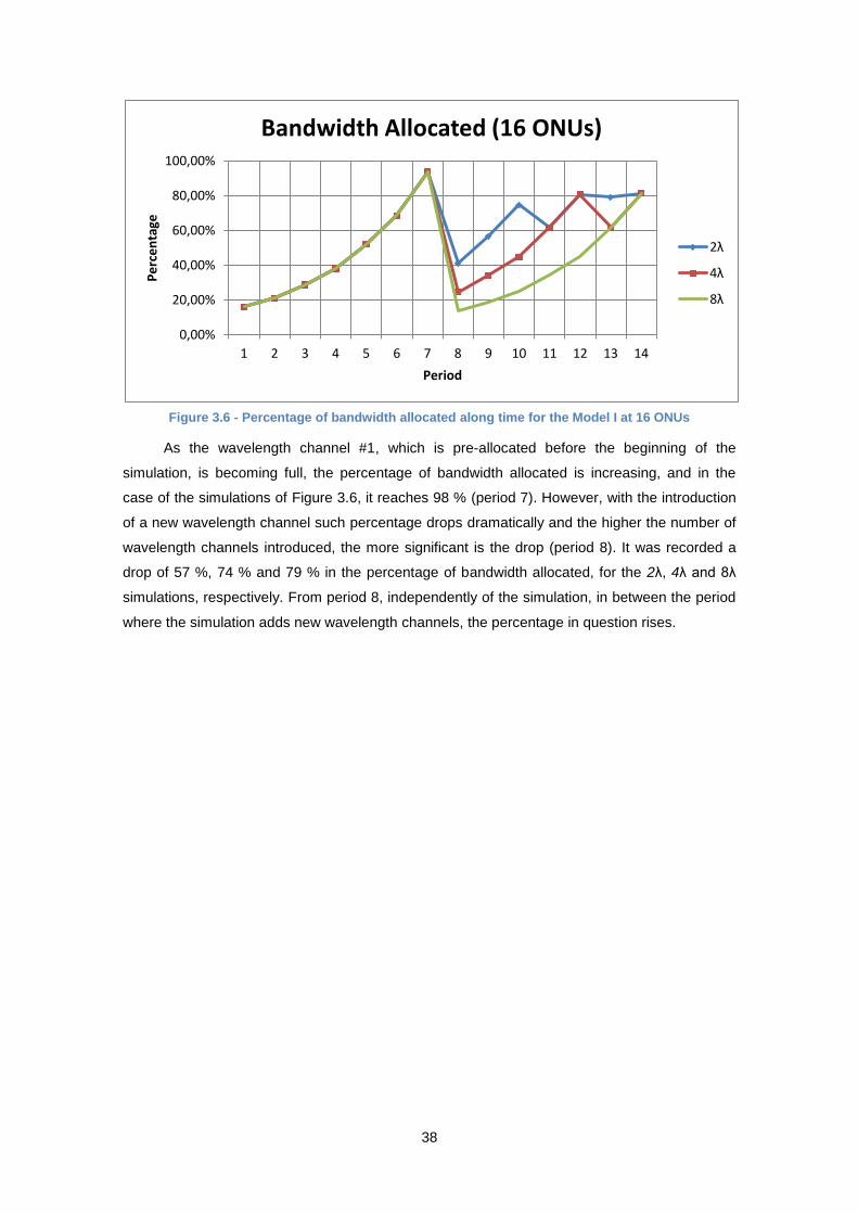
38
Figure 3.6 - Percentage of bandwidth allocated along time for the Model I at 16 ONUs
As the wavelength channel #1, which is pre-allocated before the beginning of the
simulation, is becoming full, the percentage of bandwidth allocated is increasing, and in the
case of the simulations of Figure 3.6, it reaches 98 % (period 7). However, with the introduction
of a new wavelength channel such percentage drops dramatically and the higher the number of
wavelength channels introduced, the more significant is the drop (period 8). It was recorded a
drop of 57 %, 74 % and 79 % in the percentage of bandwidth allocated, for the 2λ, 4λ and 8λ
simulations, respectively. From period 8, independently of the simulation, in between the period
where the simulation adds new wavelength channels, the percentage in question rises.
0,00%
20,00%
40,00%
60,00%
80,00%
100,00%
1 2 3 4 5 6 7 8 9 10 11 12 13 14
Pe
rce
nta
ge
Period
Bandwidth Allocated (16 ONUs)
2λ
4λ
8λ

39
Figure 3.7 - Cost and Number of upgrading ONUs along the time for the Model I at 32 ONUs
Regarding the simulations with 32 ONUs (Figure 3.7), the introduction of new wavelength
channels occurred at the fifth period, but unlike what was seen in the simulation with 16 ONUs,
the cost for that period does not represent a maximum value of cost. This happens because the
number of upgrading ONUs is big enough to rule the cost during the sixth and seventh periods.
During the seventh to the ninth period, the cost, in all simulations, goes down, following the
curves of the number of upgrading ONUs. However, the “cost@2λ” simulation needs to add
another two channels. From period 10 until period 12, simulation “cost@2λ” is adding more
channels, two at a time, as well as the simulation “cost@4λ”, but four at once. The simulation
“cost@8λ” is decreasing its value in such interval following the decrease of the number of
upgrading ONUs. Note that for the “cost@4λ” and “cost@2λ” simulations there are two peaks of
cost. The first one, when the wavelength channels are added to PON for the first time and the
second when the second wave of wavelength channels is added (starting from the period
number 9 for cost@2λ and period 11 for cost@4λ). But, unlike the case with 16 ONUs, the
second peak of cost is higher than the first one.
0 1 2 3 4 5 6 7 8 9
10 11 12 13 14 15 16 17 18 19
1 2 3 4 5 6 7 8 9 10 11 12
Co
st /
Nu
mb
er
of
Up
grad
ing
ON
Us
Period
(32 ONUs)@(Model I)
cost@2λ cost@4λ cost@8λ
#Upgrades@2λ #Upgrades@4λ #Upgrades@8λ
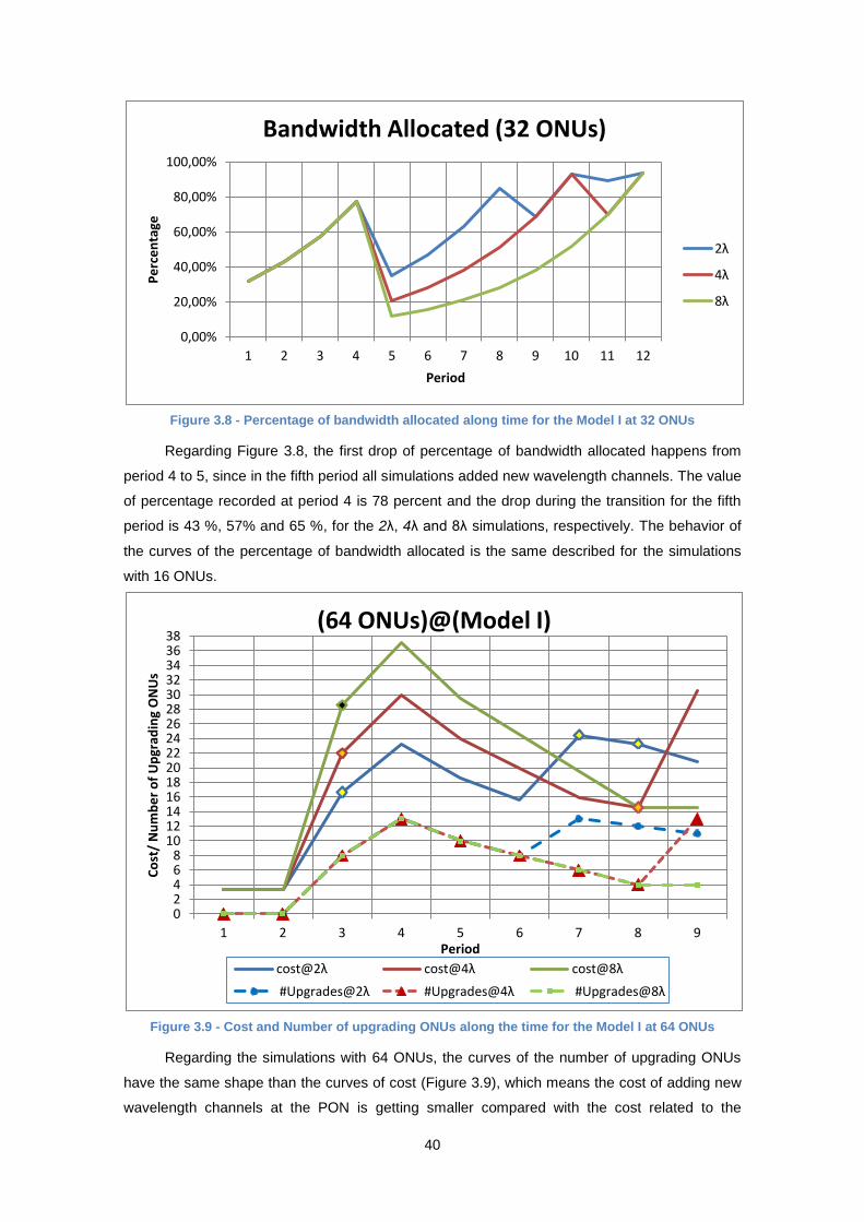
40
Figure 3.8 - Percentage of bandwidth allocated along time for the Model I at 32 ONUs
Regarding Figure 3.8, the first drop of percentage of bandwidth allocated happens from
period 4 to 5, since in the fifth period all simulations added new wavelength channels. The value
of percentage recorded at period 4 is 78 percent and the drop during the transition for the fifth
period is 43 %, 57% and 65 %, for the 2λ, 4λ and 8λ simulations, respectively. The behavior of
the curves of the percentage of bandwidth allocated is the same described for the simulations
with 16 ONUs.
Figure 3.9 - Cost and Number of upgrading ONUs along the time for the Model I at 64 ONUs
Regarding the simulations with 64 ONUs, the curves of the number of upgrading ONUs
have the same shape than the curves of cost (Figure 3.9), which means the cost of adding new
wavelength channels at the PON is getting smaller compared with the cost related to the
0,00%
20,00%
40,00%
60,00%
80,00%
100,00%
1 2 3 4 5 6 7 8 9 10 11 12
Pe
rce
nta
ge
Period
Bandwidth Allocated (32 ONUs)
2λ
4λ
8λ
0 2 4 6 8
10 12 14 16 18 20 22 24 26 28 30 32 34 36 38
1 2 3 4 5 6 7 8 9
Co
st/
Nu
mb
er
of
Up
grad
ing
ON
Us
Period
(64 ONUs)@(Model I)
cost@2λ cost@4λ cost@8λ
#Upgrades@2λ #Upgrades@4λ #Upgrades@8λ

41
upgrade of the ONUs. For example, in the simulation “cost@8λ” at the third period, the cost
related with the eight new wavelength channels at the OLT is 4 units (8*0,5) and the cost
related with the upgrade of 12 ONUs is 20 units (8*2,5). Thus, the latter is worth 20 percent of
the former. The maximum value of cost happens at period number four, in all simulations. And
the higher the number of wavelengths per tunable laser, the higher that maximum is. From the
fourth period, the simulation “cost@8λ” decreases its cost, following its curve of the number of
upgrading ONUs. Concerning the simulation “cost@2λ”, it increases the number of channels by
two in the seventh and eighth periods, whereas the simulation “cost@4λ” adds four channels in
the eighth period. The simulation with the highest wavelengths per tunable laser, “cost@8λ”,
has the highest cost from the second to the seventh period, but at the seventh period the
simulations “cost@2λ” increase its cost, becoming the highest until the eighth period because
its number of upgrading ONUs. Finally, in period nine, the simulation “cost@4λ” has the highest
cost because from period 8 to period 9 the number of ONUs has increased by 9.
Figure 3.10 - Percentage of bandwidth allocated along time for the Model I at 64 ONUs
In the graphic of the bandwidth allocated (Figure 3.10), it can be understood that the
wavelength channel #1 held the traffic demands during one period, reaching 86 percent of its
capacity. During the first wave of PON´s capacity increasing (period 3), the bandwidth allocated
dropped by 48 percent, 63 percent and 74 percent for 2λ, 4λ and 8λ simulations, respectively.
Note that the curve 2λ, does not have the same shape as its counterparts with 16 and 32 ONUs
because there are two consecutive periods, period seven and eight, where the bandwidth
allocated is going down, result of the consecutive introduction of wavelength channels in these
periods.
0,00%
10,00%
20,00%
30,00%
40,00%
50,00%
60,00%
70,00%
80,00%
90,00%
100,00%
1 2 3 4 5 6 7 8 9
Pe
rce
nta
ge
Period
Bandwidth Allocated(64 ONUs)
2λ
4λ
8λ
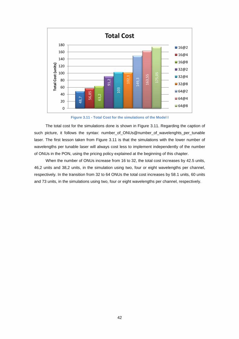
42
Figure 3.11 - Total Cost for the simulations of the Model I
The total cost for the simulations done is shown in Figure 3.11. Regarding the caption of
such picture, it follows the syntax: number_of_ONUs@number_of_wavelenghts_per_tunable
laser. The first lesson taken from Figure 3.11 is that the simulations with the lower number of
wavelengths per tunable laser will always cost less to implement independently of the number
of ONUs in the PON, using the pricing policy explained at the beginning of this chapter.
When the number of ONUs increase from 16 to 32, the total cost increases by 42.5 units,
46,2 units and 38,2 units, in the simulation using two, four or eight wavelengths per channel,
respectively. In the transition from 32 to 64 ONUs the total cost increases by 58.1 units, 60 units
and 73 units, in the simulations using two, four or eight wavelengths per channel, respectively.
48
,7
56
,85
63
,2
91
,2
10
3
10
2,1
14
9,3
16
3,5
5
17
5,0
5
0
20
40
60
80
100
120
140
160
180
Tota
l Co
st (
un
its)
Total Cost
16@2
16@4
16@8
32@2
32@4
32@8
64@2
64@4
64@8

43
3.5.2. Results for Model II
This section presents the results of the simulations for the model two, in terms of the cost
per period, number of upgrading ONUs and bandwidth allocated. Nine simulations have been
done, three for each number of ONUs tried (16, 32 and 64). Note that the simulations using
eight wavelengths per tunable laser for the model one and two are the same, since only one
type of tunable laser is used. Therefore only the simulations with two and four wavelengths per
tunable laser are going to be shown.
Figure 3.12 - Cost and Number of upgrading ONUs along the time for the Model II at 16 ONUs
Regarding Figure 3.12 the period where the first wavelengths were introduced is period
eigth, for both simulations. The simulation “cost@2λ” adds two receivers in such period, and
then, from the period 11 to period 13, one receiver is added per period and, finally, two
receivers are added in period 14. Concerning simulation “cost@4λ” in period 8, four new
wavelength channels are introduced, increasing the cost, which then goes a little bit down until
period 13, when one new wavelength channel is added. From period 13 the cost goes up
reflecting the need for new wavelength channels in the PON due to the increasing number of
upgrading ONUs. Finally, in period 14, four wavelength channels are added to the PON. In
periods 12 and 13 the simulation “cost@2λ” exceeded the “cost@4λ” because of the higher
number of upgrading ONUs in the former than the latter. Note that the introduction of
wavelengths in the second model is smoother than in model one. For example, the simulation
“cost@2λ” is increasing one wavelength channel at a time from period 11 to 13. In the same
simulation for model one (Figure 3.5),two wavelength channels were upgraded at the same time
in period 11.
0
1
2
3
4
5
6
7
8
9
10
11
1 2 3 4 5 6 7 8 9 10 11 12 13 14
Co
st/
NU
mb
er
of
Up
grad
ing
ON
Us
[ u
nit
s]
Period
(16 ONUs)@(Model II)
cost@2λ cost@4λ #Upgrades@2λ #Upgrades@4λ

44
Figure 3.13 - Percentage of bandwidth allocated along time for the Model I at 16 ONUs
The bandwidth allocated for 16 ONUs is showed in Figure 3.13. For both simulations
presented there, the wavelength channel #1 reached 93 percent of its capacity. Then, the new
wavelength channels were introduced dropping the bandwidth allocated by 52 percent and 69
percent for the simulations 2λ and 4λ, respectively. From period 8 until the end, and for both
simulations, the percentage of bandwidth allocated is going up despite the new wavelengths per
channel, but does not equal the value recorded for the seventh period. From period 12 until
period 14, the bandwidth allocated for the simulation with tunable lasers of four wavelengths
(4λ) is higher than the simulation with tunable lasers of two wavelengths (2λ), which is
something that did not happen in the first model and is the result of a softer way of introducing
the wavelength channels in the PON.
0,00%
20,00%
40,00%
60,00%
80,00%
100,00%
1 2 3 4 5 6 7 8 9 10 11 12 13 14
Pe
rce
nta
ge
Period
Bandwidth Allocated (16 ONUs)
2λ 4λ

45
Figure 3.14 - Cost and Number of upgrading ONUs along the time for the Model II at 32 ONUs
Regarding the simulations with 32 ONUs, we can see in Figure 3.14 that wavelength
channel #1 held the traffic demands by its own until the fifth period, for both simulations. Then,
the simulation “cost@2λ” added two wavelength channels and the simulation “cost@4λ” added
four wavelength channels. From period five until period 11, the mode “cost@4λ” supports all the
traffic from clients with five wavelengths, but at period 11 it needs to add another four
wavelength channels. Now, the simulation “cost@2λ”, after the fifth period, with only three
wavelength channels, supports the bandwidth demands by all ONUs until the ninth period. In
periods 9 and 10, one wavelength channel is added and in period 11, two new wavelength
channels are added. Regarding the simulation “cost@4λ” after the fifth period, only in the last
period of the simulation two new wavelengths are added.
0 1 2 3 4 5 6 7 8 9
10 11 12 13 14 15 16 17
1 2 3 4 5 6 7 8 9 10 11
Co
st/
Nu
mb
er
of
Up
grad
ing
ON
Us
[un
its]
Period
(32 ONUs)@(Model II)
cost@2λ cost@4λ #Upgrades@2λ #Upgrades@4λ

46
Figure 3.15 - Percentage of bandwidth allocated along time for the Model I at 32 ONUs
The bandwidth allocated profile for the simulations with 32 ONUs is shown in Figure
3.15.The peak of bandwidth allocated when only the wavelength channel #1 is present in the is
worth 77 percent and the consequent drop when the first new wavelength channels are
introduced is approximately 42 percent and 56 percent for the 2λ and 4λ simulations,
respectively.
Figure 3.16 - Cost and Number of upgrading ONUs along the time for the Model II at 64 ONUs
0,00%
20,00%
40,00%
60,00%
80,00%
100,00%
1 2 3 4 5 6 7 8 9 10 11
Pe
rce
nta
ge
Period
Bandwidth Allocated(32 ONUs)
2λ 4λ
0 2 4 6 8
10 12 14 16 18 20 22 24 26 28 30 32 34
1 2 3 4 5 6 7 8 9
Co
st/N
um
be
r o
f U
pgr
adin
g O
NU
s [u
nit
s]
Period
(64 ONUs )@(Model II)
cost@2λ cost@4λ #Upgrades@4λ #Upgrades@2λ

47
Figure 3.17 - Percentage of bandwidth allocated along time for the Model I at 64 ONUs
Regarding simulations using 64 ONUs, Figure 3.16 and Figure 3.17 summarize the most
important information. According to Figure 3.16, in period 3 both simulations introduced new
wavelength channels, four for the simulation “cost@4λ” and two for the simulation “cost@2λ”.
The former adds more two wavelength channels until the end of the simulation, one in period 8
and another in period 9, whereas the latter adds four more wavelength channels, one in the
seventh period, two in the eighth period and finally one in period 9. Now, regarding the
bandwidth allocated (Figure 3.17), the drop in the percentage of bandwidth allocated verified in
period 3 is worth approximately 48 percent and 63 percent for the simulations 2λ and 4λ,
respectively. From the start of that period until the end of the simulation, and for both modes,
the percentage of bandwidth allocated recovers, reaching a maximum value of 99 percentage.
Figure 3.18 - Total Cost for the simulations of the Model II
Figure 3.18 gathers the total cost for all the simulations done in this section and its
caption follows the same syntax of the one in Figure 3.11. Once again, the simulations using the
fewest number of wavelengths per tunable lasers have the lower cost, independently of the
number of ONUs in the PON. Concerning the simulation which uses tunable lasers with two
wavelengths, the transition from 16 to 32 ONUs costs 28,8 units of cost and the transition from
32 to 64 ONUs costs 74 units of cost. Now, regarding the simulation that uses tunable lasers
0,00%
20,00%
40,00%
60,00%
80,00%
100,00%
1 2 3 4 5 6 7 8 9
Pe
rce
nta
ge
Period
Bandwidth Allocated(64 ONUs)
2λ 4λ
49,3 55,9 78,1 86,8
152,1 161,8
0
50
100
150
200
Co
st
Total Cost
16@2
16@4
32@2
32@4
64@2
64@4

48
with four wavelengths, the transition from 16 to 32 ONUs costs 30,9 units of cost and the
transition from 32 to 64 ONUs cost 75,2 units.
3.5.3. Analysis
The number of upgrading ONUs at certain periods influences, most of the time, the major
piece of the cost, since the OPEX costs are one order of magnitude below the CAPEX costs.
However, when the receivers at the OLT need to be added, such profiles tend to deviate a little
bit, due to the impact of the OLT receivers cost. As the number of ONUs increase, the profile of
the cost is spreading more and more across the periods of the simulation because the number
of periods during which the legacy wavelength is enough to support the demand is decreasing,
and the average number of ONUs upgrading per period is getting higher. In the simulations with
16 ONUs, at the period where new wavelength channels are introduced in the PON, extending
the capacity of the pre-allocated wavelength, wavelength channel #1, the resulting cost is a
relative maximum, for the 2λ simulation, or even an absolute maximum, in 4λ and 8λ
simulations, whereas for the simulations with 32 and 64 ONUs it is a value on its way to a
relative or absolute maximum value of cost.
Regarding the pricing policy used and the setups tested, none of the models represent a
better cost implementation. It depends on which simulation setup the service providers want to
follow. Table 3.4 shows the cost difference between the model one and the model two (cost of
the model one minus the cost of the model two).
Setup 16@2 16@4 32@2 32@4 64@2 64@4
Diference -0,600 0,950 0,100 1,250 -2,800 1,750
Table 3.4 - Cost Difference [Model I – Model II] between the model one and two, for the initial values of Z and W
The model one is always more expensive than the model two, except in the simulations
with 32 Onus. In opposite, the simulations where tunable lasers of two wavelengths are used
tend to oscillate its decision regarding the more cost efficient model. Regarding the simulations
where the total number of upgrades performed at the client side is the same for both models,
the second model has the cheapest implementation. However, the 16@2λ and the 64@2λ
simulations do not behave the same way for the model one and two in terms of the total number
of upgrades done at the client side. This has to do with the average load per channel. The
model two tends to have a higher average load per channel than model one, since the receivers
are being added at the OLT in a smoother way. This tendency may lead to an extra upgrade of
ONUs, which is exactly what happens with the simulations mentioned previously. Regarding the
16@2λ simulation, for the model one at the eleventh period the average load per channel is
around 61 percent, whereas for the model two such quantity is 75 percent. This difference will
determine an extra upgrade of ONUs for the model two at the twelfth period. The same happens

49
in the 64@2λ simulation but this time in periods eight and nine, resulting in an extra two
upgrades done by the second model that represent the major difference in cost shown in Table
3.4.
3.6. Conclusion
In this chapter, two models were compared using a network of eight wavelengths. The
difference between them is based on the laser type used; in the first model each laser had a
specific number of wavelengths in an exclusive manner, whereas in the second the laser types
could share several wavelengths with each other. It was verified that no model was better than
the other, in term of cost, and the implementation the service provider may follow, regarding the
number of wavelengths per laser, will depend on the number of ONUs in the PON. Still,
regarding PONs evolution, the model two is softer since the profiles of the bandwidth allocated
show fewer and less significant drops when the new wavelengths are introduced in the PON.
50
4. Moving towards the 40 Gbps
technology
In this chapter, the MILP formulation #1 of the previous chapter is going to be extended in
order to provide line-rate upgrade to the wavelength channels of the Hybrid TDM/WDM PON.
As a result, some variables of the model one are introduced another index to distinguish the
different line-rates a wavelength channel can work with. The simulation of this new model will
have, as usual, three different numbers of ONUs in the PON (16, 32 and 64) and three different
numbers of wavelengths per tunable laser (2, 4 and 8). On the way to reach the results, an
improving step, regarding the MILP, is being develop and analyzed.

51
4.1. Moving the channels to 40 Gbps
The logical next step following the increasing number of wavelengths seems to be the
upgrade of the data rate from 10 Gbps to 40 Gbps. However, this transition is better said than
done as several technical challenges arise. The modulation used in 10 Gbps is the on/off
keying, since it is the cheapest and simplest. As the data rate moves to 40 Gbps, fiber non-
linear effects amplify themselves, namely the chromatic dispersion (CD) and the polarization
mode dispersion (PMD). These effects lead to pulse broadening and inter-symbol interference.
Moreover, the chirp effect starts to appear in a more regular basis if the laser is directly
modulated, contributing for signal´s spectrum broadening as well. In fact, if the on/off
modulation is used for the 40 Gbps, those three effects limit the network length to 2 kilometers,
the so called very-short-reach (VSR) optical links, which is ten times less of what we can have
for the 10 Gbps data rate.
Regarding the external modulation, the DQPSK (Differential quadrature phase shift
keying) is the modulation whose properties guarantee an excellent tolerance against chromatic
dispersion and polarization-mode dispersion for the 40 Gbps setup. In spite of this, direct
modulation is far more desirable for the access network, due to its potential for low price,
equipment compact size, low power consumption and high power characteristic when compared
with external modulators such as electro-absorption modulators and Mach-Zenger modulators.
However, in this chapter, the aforementioned problems won´t be considered.
Accordingly, this chapter deals with the allocation problem of wavelength channels, which
can have two different line rates. Note that we are still working with the CWDM grid, more
precisely with its upstream channels and the lasers used are still tunable laser.
Laser 1 (p=1 ; r=1)
Laser 2(p=2;r=1)
Laser 3
(p=3;r=1)
Laser 4(p=4;r=1)
λ1 λ2 λ3 λ4 λ5 λ6 λ7 λ8 λ9
Laser 0(p=0;r=1)
Data Rate
R1
Laser 6
(p=1,r=2)
Laser 7(p=2,r=2)
Laser 8(p=3,r=2)
Laser 9(p=4,r=2)
λ2 λ3 λ4 λ5 λ6 λ7 λ8 λ9
R2
Wavelength channels
Where R2>R1
Figure 4.1 - Wavelength channels (Upstream wavelengths), data rates and Lasers, when each tunable laser has two wavelengths per laser.
The paradigm of the problem is shown in Figure 4.1 (Using tunable laser of two
wavelengths per channel). There are nine wavelength channels, from which one is pre-
allocated, , working at R1 Gbps and it is supported by the Laser 0 (it’s not a tunable laser, it’s
a single wavelength laser coming from the old PON system,). The other eight channels, from

52
to , are going to be allocated using a simulation that is ruled by a MILP formulation and a
pricing policy (the common procedure used so far).
This paradigm is an extension of the model one from the last chapter, therefore each
tunable laser type can transmit only its own wavelengths. Two different tunable laser types
won´t use the same wavelength channels of the CWDM grid. Still, two ONUs using the same
type of tunable laser to transmit can work with the same wavelength, sharing the wavelength
channel in time.
But the problem now is that the wavelength channels can have two different line-rates,
and as presented in Figure 4.1. From such figure, note that the tunable laser 1 and tunable
laser 6 use the same wavelength channels, and . The latter works at Gbps whereas the
former works at Gbps. The same happens between the pairs Laser 2 and Laser 7, Laser 3
and laser 8, the Laser 4 and the Laser 9. In a given moment, a certain wavelength channel can
only operate with a certain data rate, or , which means only one type of laser from each
pair can be in PON at a given moment. Moreover, since , once the channel is working at
it cannot go back to work at . This means that, for example, when the laser 7 is added for
the first time, the wavelength channel #4 and #5 have been upgraded to work at ( by using
receivers for that data rate), and so the laser 2 will be discarded immediately from the network.
It was decided to restrict the wavelength channel #1 to work only at , and so only eight
wavelength channels are available to perform the upgrade from to .
At last, the goal in this chapter is to understand when the wavelength channels must be
upgraded from to and what is the impact of such upgrade in the cost and in the bandwidth
allocated per wavelength channel, given a certain PON, with a certain number of ONUs and
chosen the number of wavelength per tunable laser.
4.2. MILP Model III
The model is a simple extension of the model one from chapter 3, and only a new index
was introduced, the r index, for and for (see Figure 4.1 below the laser type
alongside with the p index). The model two is not considered in this section, because it would
be more complex and time consuming to simulate the transition for the , since it has a bigger
number of tunable laser types. Yet, using the model one, we can still have a glance of what the
transition to the 40 Gbps technology may look like in the model two.
Thus, the variables , , have the same meaning of the model one, but
the data rate discrimination is introduced by the r index. The same happens with the and
variables. Regarding the constants of this model, only three are different from the
model one of the last chapter, which are the , and , all the other remain the same.
The represents the cost of the wavelength j supported by the tunable laser I, working at
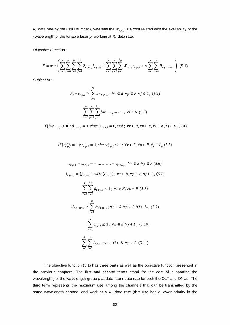
53
data rate by the ONU number i, whereas the is a cost related with the availability of the
j wavelength of the tunable laser p, working at data rate.
Objective Function :
Subject to :
The objective function (5.1) has three parts as well as the objective function presented in
the previous chapters. The first and second terms stand for the cost of supporting the
wavelength j of the wavelength group p at data rate r data rate for both the OLT and ONUs. The
third term represents the maximum use among the channels that can be transmitted by the
same wavelength channel and work at a data rate (this use has a lower priority in the

54
objective function expressed by the factor , which is a small one). So, the goal is to minimize
the cost of the equipment at the OLT and ONUs, with the awareness of the two possible data
rates with which the wavelength channels can work, while minimizing the maximum use of the
channels. From Equation (5.2) to Equation (5.9), the purpose of such constraints is the same as
the one explained for the model one of the last chapter. Equation (5.10) and Equation (5.11) are
necessary to discard the possibility of two different line rates in the same wavelength channel.
4.3. Improving the Performance of the Model III
The number of variables declared in the objective function set the dimensions of the
MILP, whereas the constraints define a polytope15
, which delimits the regions of interest for the
possible solutions of the problem. The higher the number of dimensions, the higher the number
of possible points for the optimum solution inside the polytope. There are dimensions and points
inside the polytope whose interest is time dependent and we can use this fact to reduce the
number of operations the computer´s CPU is doing. You may wonder why this optimization has
become so important this far in the thesis, after two models were already established with no
degree of optimization besides the CPLEX framework´s procedures. In fact, the computation
time has increased, from the model one and two to the model three, which was caused by the
introduction of the r index.The number of dimensions of the problem doubled as a consequence
of this transformation.
The total number of dimensions of the model three is given by the formula :
. The legacy wavelength contributes with dimensions and the other eight
wavelengths contribute with .
The wavelength channel #1 can only work at , so it contributes with dimensions
in the first term of the objective function (because can work the first channel), one
dimension in the second term (dimension responsible for the presence of that wavelength in the
OLT) and another dimension in the third term (dimension responsible to decide the traffic load
over the wavelength channel #1).
Now, the eight wavelength channels left, contribute with dimension on the first
term of the objective function ( have at its disposal 8 wavelenght channels, which can work
with one of two line data rates), 16 dimension on the second term of the objective function (note
that the wavelength channels can work at two different line rates and there are eight wavelength
channels, so one dimension is needed for each of the 16 possibilities ) and 2P dimensions on
the third term (there are P wavelength groups and the channels of each wavelength group can
work with one of two line rates).
The model three deals with the allocation of sets of wavelength receivers on the OLT
side, and tunable lasers with unshared wavelengths (From now on, =10 Gbps and =40
15
Polygon with n dimensions

55
Gbps). Yet, the way the simulation builds the MILP is quite blind, taking no advantage of
variables we bounded for the problem, like the bandwidth increasing rate from period to period.
So, the optimization idea is to simulate the model with only the dimensions it needs to
fulfill the customers´ requests in terms of bandwidth. Thus, only the minimum channels at the
OLT are going to be considered in the simulation plus an extra, enough to cope with all the
possibilities the MILP can take, at a certain period.
To accomplish that, a wider number of variables had to be taken into account by the
algorithm that built and ran the simulation, which are: the set of wavelengths allocated at 10
Gbps or 40 Gbps,as well as the set of wavelengths that have been upgraded from 10 Gbps to
40 Gbps at the previous periods. Moreover, the traffic forecast sub routine was given the ability
to recognize the sets working at 10 Gbps and at 40 Gbps needed for the next period of the
simulation, stored in the and variables, respectively. This is the critical function to
increase the number of dimensions in an “ as needed “ fashion, while not disturbing the optimal
solution.
The number of new groups of wavelengths proposed for a certain period is decided
taking into account the lowest line rate, which are the 10 Gbps wavelengths.
So, for example, if the PON needs two groups of wavelengths at 10 Gbps, then we let the
MILP choose the data rate of this sets. This means the objective function will have the
necessary variables to allocate the wavelengths channels at 10 Gbps or at 40 Gbps. By doing
this, we are actually doubling the number of dimensions that are going to be introduced in the
next period, but we keep the MILP flexible.
The normal situation of simulation for this model without any degree of improvement is
described by the procedure of Figure 3.3. However, with the improvement done for this model,
such procedure was substituted by the procedure described in Figure 4.1. Note that for this
procedure it is considered that the increasing rate of the bandwidth from period to period is
bounded from 1.3 up to 1.7, as considered in the previous chapter.
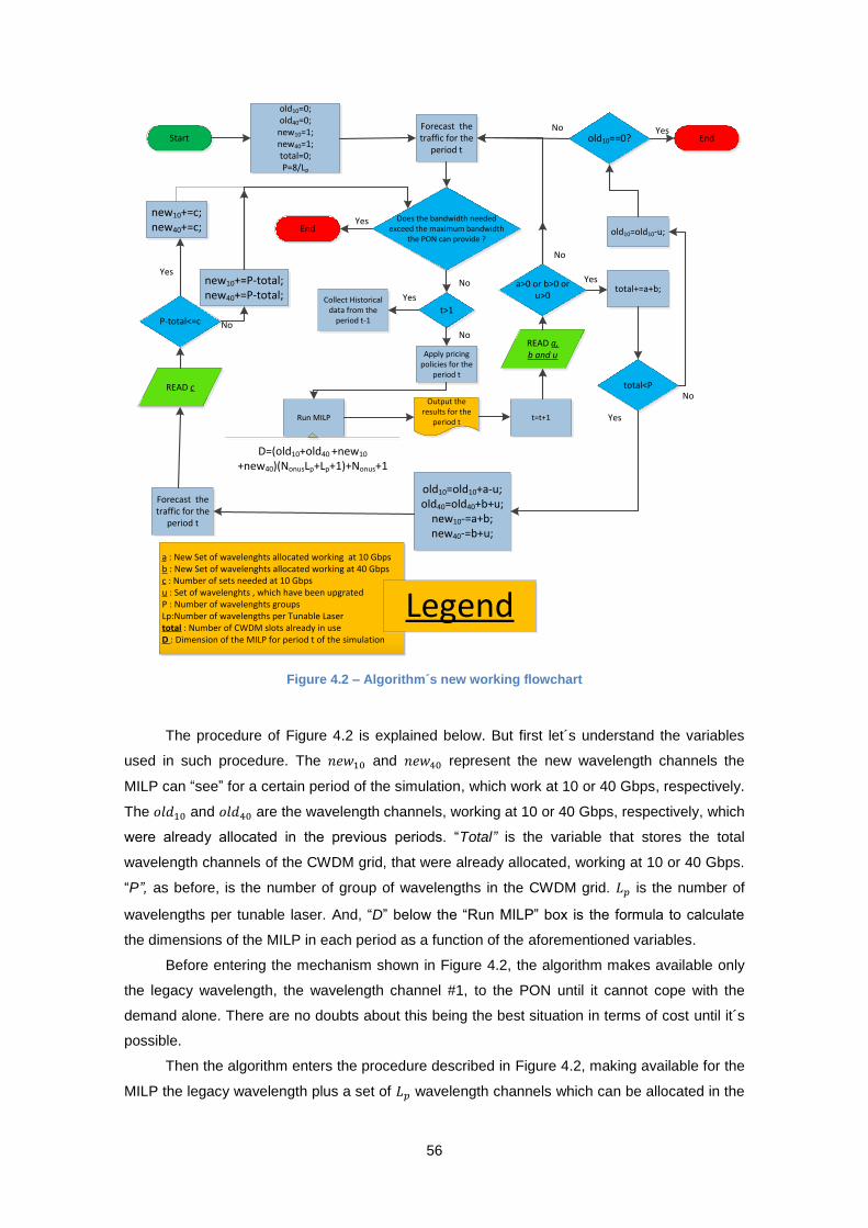
56
Start
total<P
old10=0;old40=0;
new10=1;new40=1;total=0;P=8/Lp
old10=old10+a-u;old40=old40+b+u;
new10-=a+b;new40-=b+u;
new10+=c;new40+=c;
Forecast the traffic for the
period t
READ c
P-total<=c
Yesnew10+=P-total;new40+=P-total;
No
old10=old10-u;
No
old10==0?No
EndYes
Yes
Forecast the traffic for the
period t
Does the bandwidth needed exceed the maximum bandwidth
the PON can provide ?End
t>1
Yes
No
Apply pricing policies for the
period t
Run MILP
Output the results for the
period t
Collect Historical data from the
period t-1
t=t+1
READ a, b and u
a>0 or b>0 or u>0
No
total+=a+b;Yes
Yes
No
a : New Set of wavelenghts allocated working at 10 Gbps b : New Set of wavelenghts allocated working at 40 Gbpsc : Number of sets needed at 10 Gbps u : Set of wavelenghts , which have been upgrated P : Number of wavelenghts groupsLp:Number of wavelengths per Tunable Lasertotal : Number of CWDM slots already in useD : Dimension of the MILP for period t of the simulation
Legend
D=(old10+old40 +new10
+new40)(NonusLp+Lp+1)+Nonus+1
Figure 4.2 – Algorithm´s new working flowchart
The procedure of Figure 4.2 is explained below. But first let´s understand the variables
used in such procedure. The and represent the new wavelength channels the
MILP can “see” for a certain period of the simulation, which work at 10 or 40 Gbps, respectively.
The and are the wavelength channels, working at 10 or 40 Gbps, respectively, which
were already allocated in the previous periods. “Total” is the variable that stores the total
wavelength channels of the CWDM grid, that were already allocated, working at 10 or 40 Gbps.
“P”, as before, is the number of group of wavelengths in the CWDM grid. is the number of
wavelengths per tunable laser. And, “D” below the “Run MILP” box is the formula to calculate
the dimensions of the MILP in each period as a function of the aforementioned variables.
Before entering the mechanism shown in Figure 4.2, the algorithm makes available only
the legacy wavelength, the wavelength channel #1, to the PON until it cannot cope with the
demand alone. There are no doubts about this being the best situation in terms of cost until it´s
possible.
Then the algorithm enters the procedure described in Figure 4.2, making available for the
MILP the legacy wavelength plus a set of wavelength channels which can be allocated in the
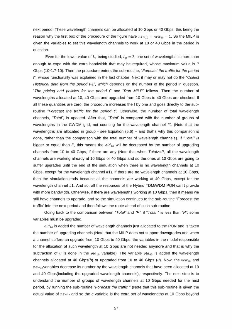
57
next period. These wavelength channels can be allocated at 10 Gbps or 40 Gbps, this being the
reason why the first box of the procedure of the figure have . So the MILP is
given the variables to set this wavelength channels to work at 10 or 40 Gbps in the period in
question.
Even for the lower value of being studied, , one set of wavelengths is more than
enough to cope with the extra bandwidth that may be required, whose maximum value is 7
Gbps (10*1.7-10). Then the procedure enters the sub-routine, “Forecast the traffic for the period
t“, whose functionally was explained in the last chapter. Next it may or may not do the “Collect
Historical data from the period t-1”, which depends on the number of the period in question.
“The pricing and policies for the period t” and “Run MILP” follows. Then the number of
wavelengths allocated at 10, 40 Gbps and upgraded from 10 Gbps to 40 Gbps are checked. If
all these quantities are zero, the procedure increases the t by one and goes directly to the sub-
routine “Forecast the traffic for the period t”. Otherwise, the number of total wavelength
channels, “Total”, is updated. After that, “Total” is compared with the number of groups of
wavelengths in the CWDM grid, not counting for the wavelength channel #1 (Note that the
wavelengths are allocated in group - see Equation (5.6) – and that´s why this comparison is
done, rather than the comparison with the total number of wavelength channels). If “Total” is
bigger or equal than P, this means the will be decreased by the number of upgrading
channels from 10 to 40 Gbps, if there are any (Note that when Total>=P, all the wavelength
channels are working already at 10 Gbps or 40 Gbps and so the ones at 10 Gbps are going to
suffer upgrades until the end of the simulation when there is no wavelength channels at 10
Gbps, except for the wavelength channel #1). If there are no wavelength channels at 10 Gbps,
then the simulation ends because all the channels are working at 40 Gbps, except for the
wavelength channel #1. And so, all the resources of the Hybrid TDM/WDM PON can´t provide
with more bandwidth. Otherwise, if there are wavelengths working at 10 Gbps, then it means we
still have channels to upgrade, and so the simulation continues to the sub-routine “Forecast the
traffic“ into the next period and then follows the route ahead of such sub-routine.
Going back to the comparison between “Total” and “P”, if “Total “ is less than “P”, some
variables must be upgraded.
is added the number of wavelength channels just allocated to the PON and is taken
the number of upgrading channels (Note that the MILP does not support downgrades and when
a channel suffers an upgrade from 10 Gbps to 40 Gbps, the variables in the model responsible
for the allocation of such wavelength at 10 Gbps are not needed anymore and that is why the
subtraction of u is done in the variable). The variable is added the wavelength
channels allocated at 40 Gbps(b) or upgraded from 10 to 40 Gbps (u). Now, the and
variables decrease its number by the wavelength channels that have been allocated at 10
and 40 Gbps(including the upgraded wavelength channels), respectively. The next step is to
understand the number of groups of wavelength channels at 10 Gbps needed for the next
period, by running the sub-routine “Forecast the traffic “ (Note that this sub-routine is given the
actual value of and so the c variable is the extra set of wavelengths at 10 Gbps beyond

58
the actual value of , but at the same time it must be guaranteed that at least one set of
wavelengths must be given to the MILP in addition to the needs of the ONUs). The value of the
variable c its taken from such-routine, the simulation will increase the number of and
by c or by the set of wavelengths left in the PON system to be allocated, in case of being
necessary. If c equals zero, nothing of that will be done. Finally, it must be seen if the total
bandwidth needed by the PON can be supplied by its channels. If not, the simulation ends. If so,
the simulation continues its main road heading to the “Collect Historical data from the previous
period”, “ Applying policies”, and so forth.
Let´s then analyze a practical case (Figure 4.3) of the optimization procedure for a
simulation with N ONUs (the number does not matter for the procedure) and with four
wavelengths per tunable laser ( ), so the simulation works with groups containing four
wavelengths, which are distributed in the CWDM grid. Therefore, the CWDM grid has two
groups of four wavelengths each.

59
10 Gbps
10/40 Gbps
λ2 λ1 λ3 λ4 λ5
40 Gbps
λ2 λ1 λ3 λ4 λ5
10
λ6 λ7 λ8 λ9
10/40 Gbps
10 /40 Gbps
λ2 λ1 λ3 λ4 λ5
10
λ6 λ7 λ8 λ9
10/40 Gbps
10 /40 Gbps
λ2 λ1 λ3 λ4 λ5
10
λ6 λ7 λ8 λ9
40 Gbps 10 /40 Gbps
λ2 λ1 λ3 λ4 λ5
10
λ6 λ7 λ8 λ9
10 /40 Gbps 40 Gbps
λ2 λ1 λ3 λ4 λ5
10
λ6 λ7 λ8 λ9
10 / 40 Gbps
40 Gbps
λ2 λ1 λ3 λ4 λ5
10
λ6 λ7 λ8 λ9
40 Gbps
End
Start
a=1 & c=1 b=1 & c=1
a=1b=1
u=1
a=1
a=b=u=0
a=b=u=0a=b=u=0
u1=1
u2=1
u1=1
a=b=u=0
u2=1
a=b=u=0Bandwidth required cannot be provided by the wavelengths of the system
a=b=u=0
D=9Nonus+ 11
D=17Nonus+ 21D=13Nonus+ 16
D=13Nonus+ 16 D=17Nonus+ 21 D=13Nonus+ 16
D=9Nonus+ 11
A
B C
D E F
G
Legend :X Gbps : Data Rate of the set
: Wavelength allocated
: Wavelength to be allocated
b=1
Figure 4.3 – State Diagram for a simulation using Lp=4 with optimization
Figure 4.3 presents the several states of a simulation setup with Lp=4. The dimensions of
such setup without optimization degree is (Note that with the optimization, such
value for dimension is the upper bound for the dimension of the MILP). Beginning at state A, we
can see that four wavelength channels were put at the disposal of the MILP to be allocated
because the wavelength #1 was full. Note that such wavelength channels can be allocated at 10
Gbps or at 40 Gbps (That information is provided by the syntax 10/40 below the channels in the
figure for state A). The dimensions of the MILP in that state are just . The MILP only
stays in this state for one period, because the wavelength channels proposed for the MILP will
certainly be allocated in the system (Remember the wavelength #1 is already full) and soon
afterwards the simulation will jump to state B or C, depending on the line rate of the first group
of wavelengths. If it was allocated at 10 Gbps, the simulation goes to state B, if it was allocated
at 40 Gbps, then the simulation jumps to state C. Note that from state A to B or C, the variable c

60
is always one for this particular case since we need to have always an extra group of
wavelength channels even if the ONUs don´t require it (This allowed us to not restrict the MILP
so much it would discard possible good solutions for the problem). In state B, the simulation has
the first group of wavelengths at 10 Gbps and gives the MILP the possibility to allocate another
group of wavelengths if needed (at 10 or 40 Gbps), whereas state C has the first group of
wavelengths working at 40 Gbps (Note that the 10 Gbps indication below the first wavelength
channel has disappeared, which means the MILP is not couting for the variables responsible for
the allocation of that wavelength group with 10 Gbps), and MILP is given the opportunity to
allocate another wavelength group if needed.
From state B and C, the simulation moves to the other states as a result of the variables
a, b and u. If all variables are zero, the program stays in the same state. If a is equal to one,
then the program jumps from state B to state E or from state C to state F. If b equals one then
the simulation moves from state B to estate D or from state C to G. Note that regarding the
variable u, if the first and second groups of wavelengths, for a certain state can be upgraded
from 10 Gbps to 40 Gbps, then the upgrade of the groups is distinguished by the index of the
variable. and are used to indicate the upgrade of the group of wavelengths one and two,
respectively. G state is always the final state of the simulation where both groups of
wavelengths are working at 40 Gbps. If the simulation is on such state and the groups of
wavelengths working at 40 Gbps cannot hold the traffic for the next period, the simulation ends.
According to the example set in Figure 4.3, if we consider that the equipment at 10 Gbps
is always most likely to be cheaper than its 40 Gbps counterparts, and the data growth factor
bounds stand still in what we’ve considered, then A and E states are most likely to rule the
major part of the simulation before it moves to the D or F state. And state A and E imply that the
simulation runs with the maximum number of dimensions possible. I could have shown the
simulation states for but the number of states is too large to be displayed in an eligible
fashion here. In that case, it would result in a softer manner of increasing the problem´s
dimensions throughout the states of the simulation.
4.4. Results and discussion
This section presents some results to illustrate the application of the methodologies
described before. In this way a C++ program has been developed, which relies on the CPLEX
framework to solve the MILP problem and runs on a Intel Core2 Duo at 2,33 GHz processor
with 2 GB of memory.
For the simulations of this chapter, several configurations will be tested, using different
numbers of ONUs (16, 32, 64) and tunable lasers with different tuning ranges and two different
line rates, and . Still, the legacy wavelength is the only wavelength
that cannot be upgraded from 10 Gbps to 40 Gbps.

61
For the models described only one type of ONU is considered, whose initial bandwidth is
100 Mbps ( ). The simulation for the MILP of this chapter uses the same paradigm
shown in Figure 3.3 and uses the same sub-routines. The sub-routine “Forecast the traffic for
the period t “ uses the same data rate increasing pace as before (from 1.3 to 1.7, according to a
uniform distribution).
The costs at the ONU and OLT depend on the data rate we are considering, according to
Table 4.1 and Table 4.2, respectively.
Equipment CAPEX Cost OPEX cost
PIN TIA Receive at 10 Gbps 0.5 0.15
PIN TIA Receive at 40 Gbps 1.5 0.20
Table 4.2 – OLT costs for the model III
The higher the data rate, the higher the cost of the optical equipment whether it is a laser
or a receiver. Moreover, the energy consumption of the equipment, usually, increases as well,
mainly due to the increase of the electronic processing speed. To map this behavior, the cost of
the laser and receiver working at 40 Gbps exceeds its 10 Gbps counterparts by a factor of
three. [27]
To calculate the it is necessary to know if the ONU i has the wavelength j of the
wavelength group (tunable laser) p working at data rate. If so (representing the
OPEX costs) or (representing the OPEX costs). Otherwise or
or if the simulation uses tunable lasers of 2, 4 or 8
wavelengths per channel, respectively; whereas or or
if the simulation uses tunable lasers of 2, 4 or 8 wavelengths per channel,
respectively.
To calculate it is necessary to know if the wavelength j of the wavelength p is
working at data rate. If so and , representing OPEX costs at the
OLT. Otherwise and ,representing CAPEX and OPEX
costs.
In this type of experience the client can be given a new transmitter working at 10 Gbps or
at 40 Gbps. That operation is called upgrade if the client had already a certain laser working at
10 Gbps and the OLT changed the data rate of the wavelengths that lasers were using and, as
CAPEX Costs OPEX Costs
CAPEX Costs OPEX Costs Laser Cost Laser Cost
2 4 8 All types 2 4 8 All types
1.5 2 2.5 0.05 4.5 6 7.5 0.075
Table 4.1 – ONU costs for the model III

62
a result, if the client is going to use the same wavelength channel he/she needs to be given a
new device that works at 40 Gbps.
On the following tables, the periods that have an asterisk are the ones when the 40 Gbps
is introduced. In such periods, one or several sets of wavelengths at the OLT were upgraded for
the 40 Gbps or were introduced to the PON using directly the 40 Gbps technology.
The periods where the 10 Gbps is, in fact, eradicated from the network are shown in red
background boxes in the following three tables (in such tables each simulation setup follows the
syntax: number_of_ONUs@number_of_wavelenghts_per_tunable-laser).
16@2 16@4 16@8
Period A16
| Cost | B17
Average
Load A |Cost| B
Average Load
A |Cost| B Average
Load
1 0 |0,95| 0 16,00% 0 |0,95| 0 16,00% 0 |0,95| 0 16,00%
2 0 |0,95| 0 21,10% 0 |0,95| 0 21,10% 0 |0,95| 0 21,10%
3 0 |0,95| 0 28,86% 0 |0,95| 0 28,86% 0 |0,95| 0 28,86%
4 0 |0,95| 0 38,14% 0 |0,95| 0 38,14% 0 |0,95| 0 38,14%
5 0 |0,95| 0 52,18% 0 |0,95| 0 52,18% 0 |0,95| 0 52,18%
6 0 |0,95| 0 68,52% 0 |0,95| 0 68,52% 0 |0,95| 0 68,52%
7 0 |0,95| 0 93,80% 0 |0,95| 0 93,80% 0 |0,95| 0 93,80%
8 3 |6,75| 0 41,04% 3|9,55| 0 13,68% 3 |13,65| 0 13,68%
9 3 |5,75| 0 56,79% 3|7,55| 0 18,93% 3 |9,65| 0 18,93%
10 2 |4,25| 0 74,61% 2 |5,55| 0 24,87% 2 |7,15| 0 24,87%
11 2 |5,55| 0 61,61% 2 |5,55| 0 34,23% 2 |7,15| 0 34,23%
12 2 |4,65| 0 80,73% 2 |5,55| 0 44,85% 2 |7,15| 0 44,85%
13 3 |7,40| 0 79,24% 2 |8,25| 0 61,63% 1 |7,15| 0 61,63%
14 3 |7,70| 0 81,45% 3 |10,15| 0 81,46% 1 |4,65| 0 81,46%
15* 4|26,55| 2 66,95% 7 |54,62| 2 40,36% 1 |119,9| 13 40,36%
16 3 |14,57| 1 88,79% 0 |2,62| 4 40,36% 0 |2,92| 1 40,36%
17 4 |28,17| 2 86,68% 1 |8,77| 1 55,16% 0 |2,92| 0 55,16%
18 0 |19,57| 7 89,27% 0 |39| 6 73,04% 1 |10,3| 0 73,04%
19 2 |24,25| 4 99,73% 0 |3,27| 5 99,73% 0 |3,3| 7 99,73%
Total 31 |161,82| 16
25 |167,08| 18
16 |202,54| 21
Table 4.3 - Information about the simulation with 16 Onus.
16
Number of ONUs receiving a new transmitter 17
Number of ONUs receiving a new transmitter following an transition from 10 Gbps to 40 Gbps
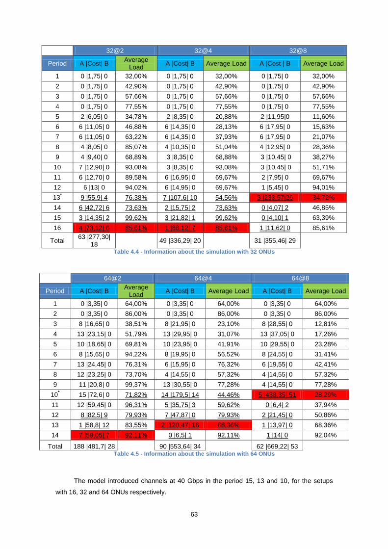
63
32@2 32@4 32@8
Period A |Cost| B Average
Load A |Cost| B Average Load A |Cost | B Average Load
1 0 |1,75| 0 32,00% 0 |1,75| 0 32,00% 0 |1,75| 0 32,00%
2 0 |1,75| 0 42,90% 0 |1,75| 0 42,90% 0 |1,75| 0 42,90%
3 0 |1,75| 0 57,66% 0 |1,75| 0 57,66% 0 |1,75| 0 57,66%
4 0 |1,75| 0 77,55% 0 |1,75| 0 77,55% 0 |1,75| 0 77,55%
5 2 |6,05| 0 34,78% 2 |8,35| 0 20,88% 2 |11,95|0 11,60%
6 6 |11,05| 0 46,88% 6 |14,35| 0 28,13% 6 |17,95| 0 15,63%
7 6 |11,05| 0 63,22% 6 |14,35| 0 37,93% 6 |17,95| 0 21,07%
8 4 |8,05| 0 85,07% 4 |10,35| 0 51,04% 4 |12,95| 0 28,36%
9 4 |9,40| 0 68,89% 3 |8,35| 0 68,88% 3 |10,45| 0 38,27%
10 7 |12,90| 0 93,08% 3 |8,35| 0 93,08% 3 |10,45| 0 51,71%
11 6 |12,70| 0 89,58% 6 |16,95| 0 69,67% 2 |7,95| 0 69,67%
12 6 |13| 0 94,02% 6 |14,95| 0 69,67% 1 |5,45| 0 94,01%
13* 9 |55,9| 4 76,38% 7 |107,6| 10 54,56% 3 |233,57|26 34,72%
14 6 |42,72| 6 73,63% 2 |15,75| 2 73,63% 0 |4,07| 2 46,85%
15 3 |14,35| 2 99,62% 3 |21,82| 1 99,62% 0 |4,10| 1 63,39%
16 4 |73,12| 6 85,61% 1 |88,12| 7 85,61% 1 |11,62| 0 85,61%
Total 63 |277,30|
18 49 |336,29| 20
31 |355,46| 29
Table 4.4 - Information about the simulation with 32 ONUs
64@2 64@4 64@8
Period A |Cost| B Average
Load A |Cost| B Average Load A |Cost| B Average Load
1 0 |3,35| 0 64,00% 0 |3,35| 0 64,00% 0 |3,35| 0 64,00%
2 0 |3,35| 0 86,00% 0 |3,35| 0 86,00% 0 |3,35| 0 86,00%
3 8 |16,65| 0 38,51% 8 |21,95| 0 23,10% 8 |28,55| 0 12,81%
4 13 |23,15| 0 51,79% 13 |29,95| 0 31,07% 13 |37,05| 0 17,26%
5 10 |18,65| 0 69,81% 10 |23,95| 0 41,91% 10 |29,55| 0 23,28%
6 8 |15,65| 0 94,22% 8 |19,95| 0 56,52% 8 |24,55| 0 31,41%
7 13 |24,45| 0 76,31% 6 |15,95| 0 76,32% 6 |19,55| 0 42,41%
8 12 |23,25| 0 73,70% 4 |14,55| 0 57,32% 4 |14,55| 0 57,32%
9 11 |20,8| 0 99,37% 13 |30,55| 0 77,28% 4 |14,55| 0 77,28%
10* 15 |72,6| 0 71,82% 14 |179,5| 14 44,46% 5 |438,35| 51 28,29%
11 12 |59,45| 0 96,31% 5 |35,75| 3 59,62% 0 |6,4| 2 37,94%
12 8 |82,5| 9 79,93% 7 |47,87| 0 79,93% 2 |21,45| 0 50,86%
13 1 |58,8| 12 83,55% 2 |120,47| 16 68,36% 1 |13,97| 0 68,36%
14 7 |59,05| 7 92,11% 0 |6,5| 1 92,11% 1 |14| 0 92,04%
Total 188 |481,7| 28
90 |553,64| 34
62 |669,22| 53 Table 4.5 - Information about the simulation with 64 ONUs
The model introduced channels at 40 Gbps in the period 15, 13 and 10, for the setups
with 16, 32 and 64 ONUs respectively.

64
Irrespective of the number of ONUs we may consider, the higher the number of
wavelengths per tunable laser, the lower the total number of exchanges at the ONU level but
the more direct is the transition from the 10 Gbps technology to the 40 Gbps, seen at the period
with the asterisks.
The immediately direct transition from the 10 Gbps to the 40 Gbps, apart from the legacy
wavelength, happens for the simulations using lasers with eight wavelengths
[sintax:numberONUs@8]. This setup for the upgrade presents serious disadvantages, as the
average load per channels column, on the tables above, is showing. The average load, after the
technological transition takes place, is lower than for the other setups, with fewer number of
wavelengths per laser, recovering one or two periods prior to the end of the simulation. This is a
quality sign demonstrating the average data rate traffic growth factor is not demanding such an
abrupt transition between the technologies in question.
It is, so, more appropriate to use the setup with tunable laser of two or four wavelengths
when we start the network with the 10 Gbps technology and aim to face the transition to the 40
Gbps technology.
Some extra information was found regarding the comparison between the periods where
the 40 Gbps technology is on the field and the periods where it is not.The ratios between the
maximum costs verified in those two parts of the simulation have an interesting pattern (Table
4.6).
16@2 16@4 16@8
Ratio 3,45 5,38 8,78
32@2 32@4 32@8
Ratio 5,63 6,35 13,01
64@2 64@4 64@8
Ratio 3,37 5,88 11,83 Table 4.6 – Ratio Between the 40 Gbps side and the 10 Gbps side of the simulations
From Table 4.6, it can be seen that the hardest transitions occur for the simulations with
32 ONUs, namely for the 32@8. However, the higher the number of wavelengths per tunable
laser, the higher is the ratio, a fact that is related with the increasing price of the tunable laser
with the number of wavelengths they can transmit. The aforementioned facts give more
consistency to what was concluded earlier, about the setups of upgrade using tunable lasers of
eight wavelengths.

65
4.5. Conclusion
This chapter started with the introduction of the problems related with the transition to the
40 Gbps technology. Then, the transformation of the MILP one was shown, enabling such
model to include the 40 Gbps technology. It was seen that this transition increased the
dimensions of the problem to almost the double, increasing the time of computation, reason why
an optimization step was created and explained. Finally, the model of this chapter was tested
with the usual number of ONUs (16, 32 and 64) and the results presented.
The main results of this chapter end up being that it is more desirable to choose the
tunable lasers with two or four wavelengths, because the way the traffic increases does not fit
very well the direct transition from 10 Gbps to 40 Gbps technology, being wasted more than 50
percent of the bandwidth during several periods.

66
5. The AWG at the Access Level
In this chapter, the paradigm of the network is radically changed from the one presented
and analyzed in the previous chapters. The arrayed waveguide grating device (AWG) is going
to be deployed at the level of the access. The cyclic property of such device is going to be
explored in order to provide an “as needed fashion” of upgrading PON in the upstream direction.

67
5.1. Introducing the problematic
The arrayed waveguide grating (AWG) is the main disruptive component of the next
generation passive optical networks, beyond implementations like the hybrid WDM/TDM PONs,
the so called long term future access networks. It can work as multiplexer/demultiplexer and as
a NxN router (Figure 5.1) [28]. As a multiplexer, the AWG combines wavelengths from different
incoming fibers to a single output fiber, increasing the capacity of the system. As a
demultiplexer, it separates the wavelengths coming from a single fiber to several output fibers.
As a NxN router the AWG performs the multiplexing and demultiplexing function at the same
time, producing an Optical Cross-Connect.
AWGλ1 , λ2 , λ3 , λ4
Demultiplexer
Multiplexer
AWG
[4x4] Router
λ1 , λ2 , λ3 , λ4
λ5 , λ6 , λ7 , λ8
λ9 , λ10 , λ11 , λ12
λ13 , λ14 , λ15 , λ16
λ1 , λ8 , λ11 , λ14
λ2 , λ5 , λ12 , λ15
λ3 , λ6 , λ9 , λ16
λ4 , λ7 , λ10 , λ13
λ1
λ2
λ3
λ4
Figure 5.1 - AWG working as Multiplexer/Demultiplexer and Router
The AWG has a cyclic behavior related with the output ports each wavelength is going to
be sent. More precisely, all wavelengths given by the formula : are
leaving the same output port of the AWG. The free spectral range (FSR) is the distance in
nanometers between two wavelengths using the same output port.
1 2 3 4 5 6 7 8 9 10
11
12
13
14
15
16
17
18
19
20
21
22
23
24
25
26
27
28
29
30
31
32
Upstream Downstream Upstream Downstream
FSR1
FSR2
FSR3
FSR4
Port 1 Port M Port 1 Port M Port 1 Port M Port 1 Port M
Figure 5.2 - FSR cyclic pattern for a 32 wavelengths and 4 FSRs and M=8
When the AWG works in a bidirectional manner, its channels are assigned to the
communication directions, the way Figure 5.2 shows and the number of free spectral ranges
reserved for the upstream is given by the formula :

68
Still, in Figure 5.2, it can be seen that the wavelength channel # 1, as well as the
wavelength channels #9, #17 and #25, uses port one, whereas the wavelength channels
#8,#16,#24 and #32 use the port M.
The AWG in the WDM-PON networks acts as a remote node, meaning the remote nodes
from other predecessor PONs (like 10GEPON, 10 GPON or even Hybrid WDM/TDM PONs)
need to be replaced. Two problems arise from this replacement. The price of the AWG is far
higher than the cost of a power splitter. For example, the 1:32 AWG costs more than four times
the value of a 1:32 power splitter. Moreover, the AWG behavior depends on the temperature,
and so, the remote node location might need to be thermally conditioned, which is certainly not
the right path to follow due to OPEX costs ( manly maintenance and energy costs).
To overcome these drawbacks, AWGs are placed in the Central Office, where the OLTs
are located, minimizing the number of AWGs in the network.
This type of evolution implies changes at the OLT, more precisely, on the type of
wavelength channels involved because we are going to use DWDM channels (The standard
AWGs work within a narrow band where the DWDM grid is applied [25]). The ONUs need to be
changed in order to use DWDM transmitters. AWGs have an insertion loss below 3 dB and do
not depend on the number of output ports they have, which is an important feature, so they do
not change in a dramatic way the power budget needed for the communication.
OLTAWG
(1:M)
1
2
3
4
1
2
3
4
1
2
3
4
. . .
. . .
Central Office
. . .
λ2 λ18
λ1 λ17
λ8 λ24
Splitter Level – Using a
Splitter factor of N/M
ONU Level – N ONUs in
total
Figure 5.3 - Network Architecture
So, the idea (Figure 5.3) is to keep the optical distribution network (ODN) the way it
always has been (the power splitters are still used as remote nodes), changing the edges of the
69
networks in an “as needed“ fashion taking advantage of the free spectral range of the AWG.
The ONUs linked to the same power splitter share the same wavelengths, but the number of
available wavelengths can be increased if the AWG has more than one FSR for the upstream
channels and if needed. So, the ONUs start with a specific transmitter corresponding to the
wavelengths they can use, which depend on the power splitter each ONU is physically linked
and, when needed, they can be given other transmitters whose working wavelengths are
separated, in nanometers, by the least integer possible of FSRs from the first wavelength
assigned inside a region of channels destined for the upstream communication.
In Figure 5.3, three groups of ONUs are shown (blue, yellow and green). At the
beginning, each group can work with only one wavelength channel dedicated to the group. The
blue group works with wavelength channel #1, the yellow group works with wavelength channel
#2, and the green group works with the wavelength channel #8. Nevertheless, when necessary
each of the previous groups will be given another dedicated wavelength channels. The blue
group is given the wavelength channel #17, the yellow group is given the wavelength channel
#18 and the wavelength channel # 24 is allocated to the green group. (Note that the allocation
of the wavelength channel for the upstream in Figure 5.3 follows the grid presented in Figure
5.2).
In summation, this problematic deals with the allocation of DWDM receiver at the OLTs
and single wavelength transmitter at the ONUs for the paradigm presented in Figure 5.2.
5.2. MILP Model Number IV
Variables:
binary variable that is one if jth wavelength is supported in the network;
binary variable that is one if ONU i is using the j wavelength;
binary variable that is one if the ONU i is using the output port m of the AWG.
integer that represents the maximum traffic load value for the m port of the
AWG;
Constants:
set of output ports of the AWG;
number of free spectral ranges for the upstream;
is cost at the OLT related with the utilization of wavelength j;
set of ONUs inside the passive optical network;
cost of the wavelength j at the ONU i;
set of wavelengths that can flow through the m AWG port;
set of wavelengths that can be used by the network;
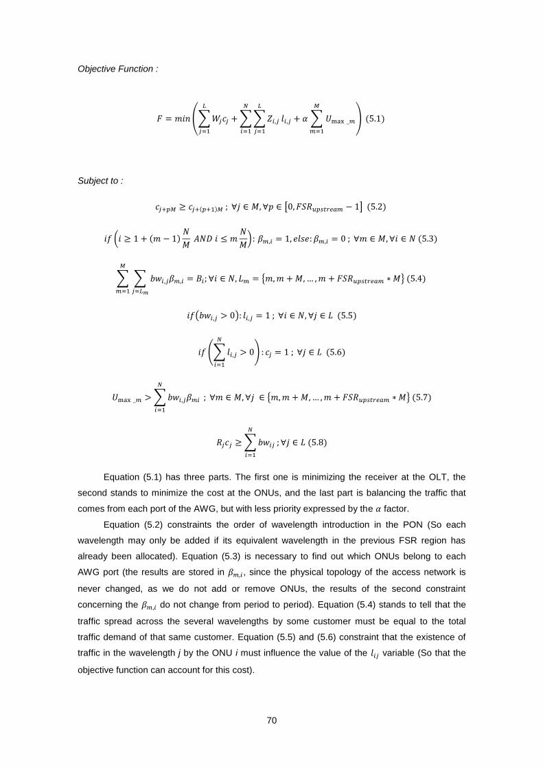
70
Objective Function :
Subject to :
Equation (5.1) has three parts. The first one is minimizing the receiver at the OLT, the
second stands to minimize the cost at the ONUs, and the last part is balancing the traffic that
comes from each port of the AWG, but with less priority expressed by the factor.
Equation (5.2) constraints the order of wavelength introduction in the PON (So each
wavelength may only be added if its equivalent wavelength in the previous FSR region has
already been allocated). Equation (5.3) is necessary to find out which ONUs belong to each
AWG port (the results are stored in , since the physical topology of the access network is
never changed, as we do not add or remove ONUs, the results of the second constraint
concerning the do not change from period to period). Equation (5.4) stands to tell that the
traffic spread across the several wavelengths by some customer must be equal to the total
traffic demand of that same customer. Equation (5.5) and (5.6) constraint that the existence of
traffic in the wavelength j by the ONU i must influence the value of the variable (So that the
objective function can account for this cost).

71
Equation (5.7) guarantees that the variable ends with the maximum value of the
load over the wavelength that flows through the port m of the AWG. Finally, the Equation (5.8)
imposes that the resources must be available in the PON system to guarantee the OLT copes
with all the traffic demands by the customers.
5.3. Results and Discussion
This section presents some results to illustrate the application of the methodologies
described.In this way a C++ program has been developed, which relies on the CPLEX
framework to solve the MILP problem and runs on an Intel Core2 Duo at 2,33 GHz processor with
2 GB of memory.
For the simulations of this chapter, several configurations will be tested, using different
numbers of ONUs (16, 32, and 64) and tunable lasers with different tuning ranges.
For the model described before, only one type of ONU is considered, whose initial bandwidth
is 100 Mbps ( ). The simulation for the MILP of this chapter uses the same paradigm
shown in Figure 3.3 and uses the same sub-routines. The sub-routine “Forecast the traffic for
the period t “ uses the same data rate increasing pace (from 1.3 to 1.7, according with a uniform
distribution ).
The most common commercial AWGs[25] use 32 channels of 100 Ghz (0,8 nm) of
bandwidth each, more than enough reason to use this equipment as a reference for the
simulations.
The costs the ILP will consider have a relative nature and the reference equipment is the
10 Gbps DWDM transmitters. The CAPEX cost of the receivers and transmitter is the same as
in the previous chapters. The OPEX costs have suffered a ten percent aggravation for both the
receivers and transmitters because the DWDM channels demand mechanisms to avoid
wavelength drifts. The procedure shown in Figure 3.3 was reused for the MILP of this chapter.
Cost OPEX CAPEX
Equipment
10 Gbps DWDM receivers 0,165 0,5
10 Gbps DWDM transmitters 0,055 1
Table 5.1 - Equipment OPEX and CAPEX costs
To calculate the it is necessary to know if the ONU i has the wavelength j. If so,
(representing the OPEX costs). Otherwise, (CAPEX + OPEX cost).
Now, to calculate the , it is necessary to know if the wavelength j is allocated in the system. If
so, (representing the OPEX costs), otherwise (CAPEX+OPEX
cost).
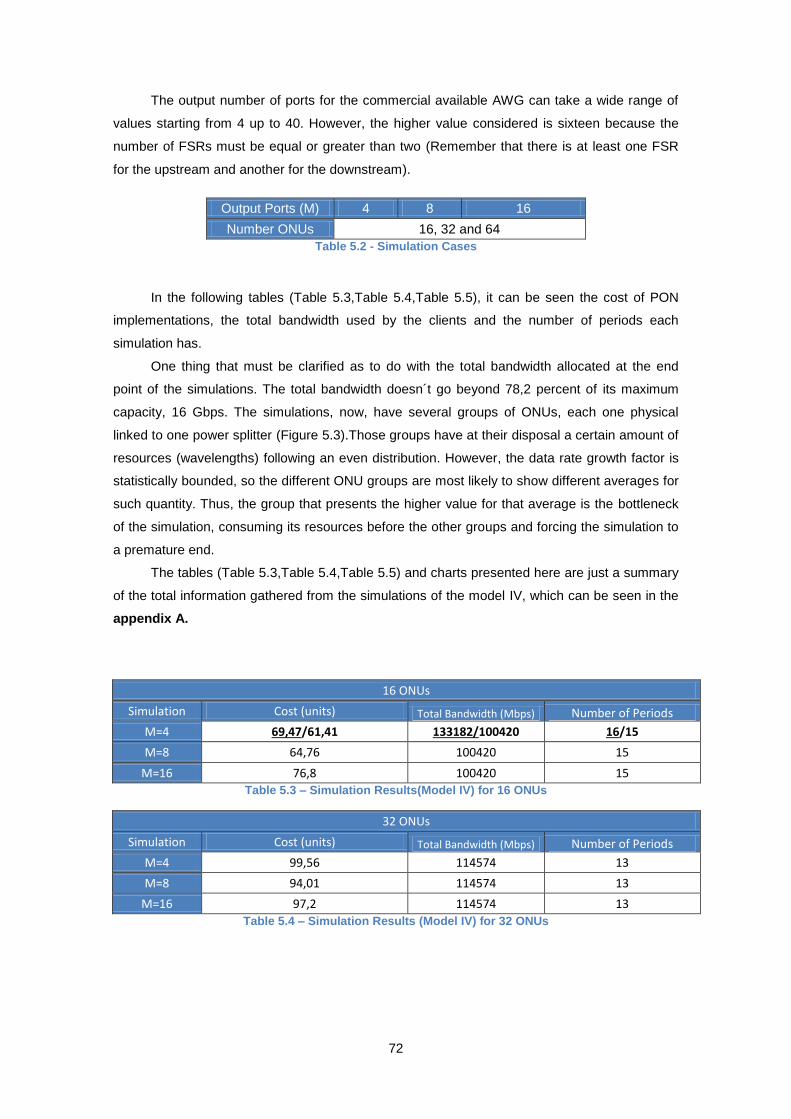
72
The output number of ports for the commercial available AWG can take a wide range of
values starting from 4 up to 40. However, the higher value considered is sixteen because the
number of FSRs must be equal or greater than two (Remember that there is at least one FSR
for the upstream and another for the downstream).
Output Ports (M) 4 8 16
Number ONUs 16, 32 and 64
Table 5.2 - Simulation Cases
In the following tables (Table 5.3,Table 5.4,Table 5.5), it can be seen the cost of PON
implementations, the total bandwidth used by the clients and the number of periods each
simulation has.
One thing that must be clarified as to do with the total bandwidth allocated at the end
point of the simulations. The total bandwidth doesn´t go beyond 78,2 percent of its maximum
capacity, 16 Gbps. The simulations, now, have several groups of ONUs, each one physical
linked to one power splitter (Figure 5.3).Those groups have at their disposal a certain amount of
resources (wavelengths) following an even distribution. However, the data rate growth factor is
statistically bounded, so the different ONU groups are most likely to show different averages for
such quantity. Thus, the group that presents the higher value for that average is the bottleneck
of the simulation, consuming its resources before the other groups and forcing the simulation to
a premature end.
The tables (Table 5.3,Table 5.4,Table 5.5) and charts presented here are just a summary
of the total information gathered from the simulations of the model IV, which can be seen in the
appendix A.
16 ONUs
Simulation Cost (units) Total Bandwidth (Mbps) Number of Periods
M=4 69,47/61,41 133182/100420 16/15
M=8 64,76 100420 15
M=16 76,8 100420 15
Table 5.3 – Simulation Results(Model IV) for 16 ONUs
32 ONUs
Simulation Cost (units) Total Bandwidth (Mbps) Number of Periods
M=4 99,56 114574 13
M=8 94,01 114574 13
M=16 97,2 114574 13
Table 5.4 – Simulation Results (Model IV) for 32 ONUs

73
64 ONUs
Simulation Cost (units) Total Bandwidth (Mbps) Number of Periods
M=4 154,03 125196 11
M=8 152,71 125197 11
M=16 139,76 125297 11
Table 5.5 – Simulation Results (Model IV) for 64 ONUs
Concerning the simulation with 16 ONUs using one AWG with four output ports, it has
simulated one more period than for the other number of ports per AWG. However, to provide
the comparison between the other setups regarding the cost, the number of periods was limited
to fifteen.
Figure 5.4 - Average Load of the channels (Model IV) for 16 ONUs
Figure 5.5 - Average Load of the channels (Model IV) for 32 ONUs
0,0%
10,0%
20,0%
30,0%
40,0%
50,0%
60,0%
70,0%
80,0%
90,0%
1 2 3 4 5 6 7 8 9 10 11 12 13 14 15 16
Pe
rce
nta
ge
Period
Bandwidth Allocated (16 ONUs)
M=4 @ 16 ONUs M=8 @ 16ONUs M=16 @ 16ONUs
0,00%
20,00%
40,00%
60,00%
80,00%
100,00%
1 2 3 4 5 6 7 8 9 10 11 12 13
Pe
rce
nta
ge
Period
Bandwidth Allocated (32 ONUs)
M=4 @ 32 ONUs M=8 @ 32 ONUs M=16 @ 32ONUs

74
Figure 5.6 - Average Load of the Channels (Model IV) for 64 ONUs
Concerning the simulation with 16 ONUs (Table 5.3) the cost is getting higher as the
number of AWG ports (M) increase. In respect to the simulations with the 32 ONUs (Table 5.4),
such quantity, initially goes down and then goes up. Finally, when 64 ONUs (Table 5.5) are
brought into the picture, the cost drops considerably. Let´s understand why. A larger number of
ports (M) means a higher number of wavelengths available at the beginning of the simulation
(so, groups of ONUs with fewer ONUs) as well as a higher initial CAPEX cost and a consequent
higher OPEX cost to maintain those wavelengths. On the other hand, as the number of ports of
the AWG are reduced, there are more moments when the simulation needs to add other
wavelengths, which are responsible for extra CAPEX investment beyond the initial investment.
Regarding the simulations with 16 ONUs, as the number of output ports rise, the initial
CAPEX investment and subsequent OPEX cost compensates all the initial CAPEX, OPEX and
extra CAPEX investments for the simulations using AWGs with fewer ports.
Now, concerning the simulations with 32 ONUs (Table 5.4), the decrease of the extra
number of CAPEX investments, when we pass from M=4 to M=8, is the main element that
drives the reduction of the overall cost seen in that transition. However, the increase of the
OPEX cost when we move to the simulation with M=16, which is of about 1.32 units per period
in relation to the simulation with M=8, alongside the significant increase of the total initial cost
(cost for the first period), contributes to rise the overall cost of this specific simulation setup.
Regarding the simulations with 64 ONUs (Table 5.5), the mean value of the extra CAPEX
investments per period, for those periods where it was needed, has increased in relation to the
other simulations with fewer ONUs. The aforementioned considerations alongside with the fact
that the difference in OPEX costs between two simulations with the same number of ONUs is
0,00%
10,00%
20,00%
30,00%
40,00%
50,00%
60,00%
70,00%
80,00%
90,00%
100,00%
1 2 3 4 5 6 7 8 9 10 11
Pe
rce
nta
ge
Period
Bandwidth Allocated ( 64 ONUs )
M=4 @ 64ONUs M=8 @ 64ONUs M=16 @ 64 ONUs

75
constant, (given by , where is the difference in ports between the AWGs of the
simulations) results in a decreasing cost alongside the reducing number of ports of the AWG.
Regarding the bandwidth allocated to the clients, independently of the number of ONUs,
the higher the number of ports of the AWG used, the lower is the average occupation of the
channels, as expected.
Back to the costs, it was not considered the cost of the AWG element, and so the total
costs presented here (Table 5.3,Table 5.4 and Table 5.5) for the nine simulations and the
relations between them, may be influenced, more particularly the simulation with 32 and 64
ONUs. If the cost of the AWG is most likely to increase with the number of its output ports, then
the simulations with 32 and 64 ONUs may suffer a turnaround regarding the AWG type that
guarantees the cheaper implementation, since for these simulations the total costs seen in
Table 5.4 and Table 5.5, do not rise in a linear way according to the number of ports.
5.4. Conclusion
In this chapter, it was studied and analyzed the introduction of one disruptive component
in the passive optical network, the AWG. The best location for it was decided to be the OLT,
guaranteeing the reduction of both OPEX and CAPEX, the latter by reducing the number of
AWGs needed. The cyclic property of the AWGs was then explored to give the service provider
the opportunity to assign bandwidth to the customers in an “as needed” fashion. The variables
that we could change for the simulations were the number of ports of the AWG and the total
number of ONUs in the system. Those two elements were combined finding out a total of nine
combinations. With those nine simulations, it was found that the cost of the implementations
does not follow the same behavior when the number of ports of the AWG is varied for the
number of ONUs tried. This fact had a lot to do with the number of extra CAPEX investments
and as well as the amount of such investments. Regarding the average load of the channels,
the higher the number of ports of the AWG, the lower is that quantity independently of the
number of ONUs in the PON.

76
6. Conclusions and Future Work
6.1. Conclusions
In this thesis, four paradigms of passive optical network were studied in different levels,
with the main focus being placed on the upstream channels. The main goal was always to
generate several setups for each paradigm seeking the understanding of the behavior of the
cost and bandwidth allocated.
Each of those paradigms, related to the uplink channels of PONs, were built using ILP
formulations, since these formulations can be formulated seeking the cheapest cost using one
pricing policy.
The first paradigm came from the reference [24], and its scope was extended by varying
the number of clients in the PON. Part of the results from such paper were confirmed, such as
the traffic occupation per channel although the wavelength allocation pattern did not match
exactly. It was also found out that for 64 ONUs, the total cost of the implementation was lower
than what was expected by 10 units of cost.
The second paradigm included the CWDM grid at the access network, which proved to
be a good possibility to follow due to the maturity of the CWDM components. The paradigm was
sub-divided in two models whose common characteristic is the use of tunable lasers. What set
those models apart is the way the tunable lasers are distributed along the CWDM grid. In the
first model, each tunable laser type had a single piece of the grid; in the second model each
tunable laser type may share wavelengths of the grid with other tunable laser types. Inside each
mode, several setups were tested, contemplating different number of ONUs in the PON and
different number of wavelengths per tunable laser. It was found out that the simulations with
fewer numbers of wavelengths per tunable laser cost less to implement for both models. More
frequently, the model two is cheaper to implement (but not by much) although it´s more complex
to manage because of a larger number of wavelength types.
With the previously mentioned paradigms, it was shown three models with a good
capability of being the middle term evolution for the actual passive optical networks, since in all
of them it is provided backward compatibility with the legacy system (which is a PON with one
wavelength per direction working at 10 Gbps).
The next step performed in the thesis was to understand how the model one of the
second paradigm would perform while facing the transition for the 40 Gbps, resulting in another
ILP model. It was used a cost factor of three between both technologies (10 Gbps and 40
Gbps). The conclusion about this model was that for the bandwidth increasing factor used
(between 1.3 and 1.7) the tunable lasers with two wavelengths per channel provided the softer
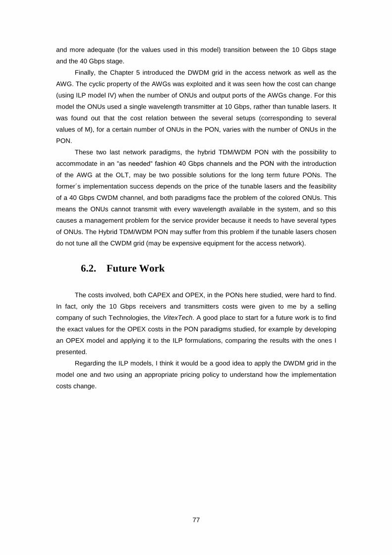
77
and more adequate (for the values used in this model) transition between the 10 Gbps stage
and the 40 Gbps stage.
Finally, the Chapter 5 introduced the DWDM grid in the access network as well as the
AWG. The cyclic property of the AWGs was exploited and it was seen how the cost can change
(using ILP model IV) when the number of ONUs and output ports of the AWGs change. For this
model the ONUs used a single wavelength transmitter at 10 Gbps, rather than tunable lasers. It
was found out that the cost relation between the several setups (corresponding to several
values of M), for a certain number of ONUs in the PON, varies with the number of ONUs in the
PON.
These two last network paradigms, the hybrid TDM/WDM PON with the possibility to
accommodate in an “as needed“ fashion 40 Gbps channels and the PON with the introduction
of the AWG at the OLT, may be two possible solutions for the long term future PONs. The
former´s implementation success depends on the price of the tunable lasers and the feasibility
of a 40 Gbps CWDM channel, and both paradigms face the problem of the colored ONUs. This
means the ONUs cannot transmit with every wavelength available in the system, and so this
causes a management problem for the service provider because it needs to have several types
of ONUs. The Hybrid TDM/WDM PON may suffer from this problem if the tunable lasers chosen
do not tune all the CWDM grid (may be expensive equipment for the access network).
6.2. Future Work
The costs involved, both CAPEX and OPEX, in the PONs here studied, were hard to find.
In fact, only the 10 Gbps receivers and transmitters costs were given to me by a selling
company of such Technologies, the VitexTech. A good place to start for a future work is to find
the exact values for the OPEX costs in the PON paradigms studied, for example by developing
an OPEX model and applying it to the ILP formulations, comparing the results with the ones I
presented.
Regarding the ILP models, I think it would be a good idea to apply the DWDM grid in the
model one and two using an appropriate pricing policy to understand how the implementation
costs change.

78
References
[1] FiberOptics.info, Applications in the Real World, 2008. [Online]. Available at: http://www.fiber-optics.info/history/P3/. [Accessed: 05-Aug-2012].
[2] Lan,Cedric F., Passive optical networks: principles and practice. Academic Press, San Diego, California, USA, 2007.
[3] Keiser,Gerb , FTTX Concepts and Applications. John Wiley & Sons, Hoboken, NJ, USA, 2006.
[4] Connectedhome2go.com, Nielson´s Law, 2008. [Online]. Available at: http://connectedhome2go.com/2008/03/18/nielsens-law/. [Accessed: 07-Sep-2012].
[5] Genexis.eu, Point-to-Point FTTH network, 2011. [Online]. Available: http://www.genexis.eu/ftth-technologies/point-to-point. [Accessed: 07-Sep-2012].
[6] FSAN, Broadband optical access systems based on Passive Optical Networks, ITU-T G983.1 Recommendation, 2005.
[7] FSAN, A broadband optical access system with enhanced survivability, ITU-T G.983.5 Recommendation, 2002.
[8] FSAN, A broadband optical access system with increased service capability by wavelength allocation, ITU-T G.983.3 Recommendation, 2001.
[9] FSAN, A broadband optical access system with increased service capability using dynamic bandwidth assignment, ITU-T G.983.4 Recommendation, 2001.
[10] FSAN, Gigabit-capable Passive optical Netwoks(G-PON): Transmission convergence layer specification, ITU-T G.984.3 Recommendation, 2008.
[11] FSAN, Gigabit-capable Passive Optical Networks (GPON):Physical Media Dependent(PMD) layer specification, ITU-T G.984.2 Recommendation, 2003.
[12] FSAN, Gigabit-capable Passive Optical Networks (GPON): General characteristics, ITU-T G.984.1 Recommendation, 2008.
[13] FSAN, Gigabit-capable Passive Optical Networks(G-PON): ONT management and control interface specification, ITU-T G.984.4 Recommendation, 2008.
[14] Kramer, G. , "Ethernet Passive Optical Network (EPON): Building a Next-Generation Optical Access Network", IEEE communication Magazine, vol. 40, no.2, pp. 66–73, Feb. 2002.
[15] M. Hajduczenia, and P. R. M. Inácio, "10G EPON Standardization in IEEE 802.3av" Project,OFC/NFOEC, San Diego, USA, Feb.2008
[16] Haran, Onn, White Paper Ethernet in the First Mile : New Ethernet Capabilities Enable Low-cost Triple-Play Services. pp. 1–14, April 2006.
[17] FSAN, 10-Gigabit-capable passive optical networks(XG-PON): General requirements, Itu-T G987.1 Recommendation, 2010.

79
[18] FSAN, 10-Gigabit-capable passive optical networks(XG-PON): Physical media dependent(PMD) layer specification, ITU-T G.987.2 Recommendation, 2010.
[19] FSAN, 10-Gigabit-capable passive optical networks(XG-PON): Transmission convergence (TC) layer specification, ITU-T G.987.3 Recommendation, 2010.
[20] S. Jain, F. Effenberger, A. Szabo, Z. Feng, A. Forcucci, W. Guo, Y. Luo, R. Mapes, Y. Zhang, and V. O. Byrne, "World’s First XG-PON Field Trial", Jornal of Lightwave Technology, vol. 29, no. 4, pp. 524–528, Feb. 2011.
[21] M. de Andrade et al, “Evaluating Strategies for Evolution of Passive Optical Networks (PON)”, IEEE Communcations Magazine, pp. 176–184, July 2011.
[22] Eira, António, Planeamento e Concepção de Redes de Acesso Ópticas de Nova Geração Engenharia Electrotécnica e de Computadores, Instituto Superior Técnico, October 2010.
[23] N.Cheng, G Wei, and F. Effenbeger, "Dynamic Spectrum Managed Passive Optical Networks", IEEE Communcations Magazine, p. 86-93,. Nov. 2011.
[24] M. De Andrade, M. Tornatore, S. Sallent, and B. Mukherjee, "Optimizing the Migration to Future-Generation Passive Optical Networks (PON)", IEEE System Journal, vol. 4, no. 4, pp. 413–423, Dec. 2010.
[25] C. Bock, J. Prat, and S. D. Walker, "Hybrid WDM / TDM PON Using the AWG FSR and Featuring Centralized Light Generation and Dynamic Bandwidth Allocation",Jornal of Lightwave Technology, vol. 23, no. 12, pp. 3981–3988, Dec. 2005.
[26] www.santec.com, Tunable Laser TSL-510. [Online]. Available at: http://www.santec.com/en/products/instruments/tsl-510?gclid=CM2zpvbh3rMCFU3HtAod2kUAbQ. [Accessed: 06-Oct-2012].
[27] R. Huelsermann, M. Gunkel, C. Meusburger, and D. A. Schupke, "Cost modeling and evaluation of capital expenditures in optical multilayer networks", Journal of Optical Networking, vol. 7, no. 9, p. 814-832, Aug. 2008.
[28] Wong, E., "Next-Generation Broadband Access Networks and Technologies", Journal of Lightwave Technology, vol. 30, no. 4, pp. 597–608, Feb. 2012.

80
A. Information about the simulation
of the MILP Model IV
The syntax used for the title of the tables of this section follow the next : A@B. Where the
A is the number of output ports of the AWG and the B is the number of ONUs of the
simulation.
4@16
Period Demanded Bandwidth [Mbps] Cost Average Load Number Of Wavelengths
1 1600 19,54 4,0%
4
2 2140 1,54 5,4%
3 2886 1,54 7,2%
4 3814 1,54 9,5%
5 5218 1,54 13,0%
6 6852 1,54 17,1%
7 9380 1,54 23,5%
8 12312 1,54 30,8%
9 17037 1,54 42,6%
10 22384 1,54 56,0%
11 30807 1,54 77,0%
12 40366 4,87 67,3% 6
13 55470 7,2 69,3% 8
14 73311 5,86 81,5% 9
15 100420 8,58 83,7% 12
16 133182 8,02 88,8% 15
Total 69,47
Table A.1 – Simulation information, M=4 and 16 ONUs (Model IV)
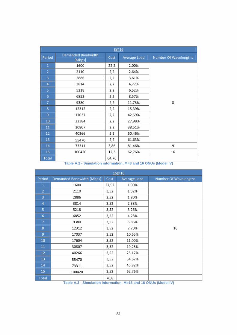
81
8@16
Period Demanded Bandwidth
[Mbps] Cost Average Load Number Of Wavelengths
1 1600 22,2 2,00%
8
2 2110 2,2 2,64%
3 2886 2,2 3,61%
4 3814 2,2 4,77%
5 5218 2,2 6,52%
6 6852 2,2 8,57%
7 9380 2,2 11,73%
8 12312 2,2 15,39%
9 17037 2,2 42,59%
10 22384 2,2 27,98%
11 30807 2,2 38,51%
12 40366 2,2 50,46%
13 55470 2,2 61,63%
14 73311 3,86 81,46% 9
15 100420 12,3 62,76% 16
Total 64,76
Table A.2 - Simulation information, M=8 and 16 ONUs (Model IV)
16@16
Period Demanded Bandwidth [Mbps] Cost Average Load Number Of Wavelengths
1 1600 27,52 1,00%
16
2 2110 3,52 1,32%
3 2886 3,52 1,80%
4 3814 3,52 2,38%
5 5218 3,52 3,26%
6 6852 3,52 4,28%
7 9380 3,52 5,86%
8 12312 3,52 7,70%
9 17037 3,52 10,65%
10 17604 3,52 11,00%
11 30807 3,52 19,25%
12 40266 3,52 25,17%
13 55470 3,52 34,67%
14 73311 3,52 45,82%
15 100420 3,52 62,76%
Total 76,8 Table A.3 - Simulation information, M=16 and 16 ONUs (Model IV)
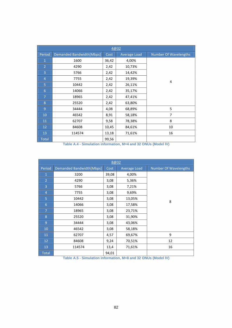
82
4@32
Period Demanded Bandwidth[Mbps] Cost Average Load Number Of Wavelengths
1 1600 36,42 4,00%
4
2 4290 2,42 10,73%
3 5766 2,42 14,42%
4 7755 2,42 19,39%
5 10442 2,42 26,11%
6 14066 2,42 35,17%
7 18965 2,42 47,41%
8 25520 2,42 63,80%
9 34444 4,08 68,89% 5
10 46542 8,91 58,18% 7
11 62707 9,58 78,38% 8
12 84608 10,45 84,61% 10
13 114574 13,18 71,61% 16
Total 99,56
Table A.4 - Simulation information, M=4 and 32 ONUs (Model IV)
8@32
Period Demanded Bandwidth[Mbps] Cost Average Load Number Of Wavelengths
1 3200 39,08 4,00%
8
2 4290 3,08 5,36%
3 5766 3,08 7,21%
4 7755 3,08 9,69%
5 10442 3,08 13,05%
6 14066 3,08 17,58%
7 18965 3,08 23,71%
8 25520 3,08 31,90%
9 34444 3,08 43,06%
10 46542 3,08 58,18%
11 62707 4,57 69,67% 9
12 84608 9,24 70,51% 12
13 114574 13,4 71,61% 16
Total 94,01
Table A.5 - Simulation information, M=8 and 32 ONUs (Model IV)

83
16@32
Period Demanded Bandwidth[Mbps] Cost Average Load Number Of Wavelengths
1 3200 44,4 2,00%
16
2 4290 4,4 2,68%
3 5766 4,4 3,60%
4 7287 4,4 4,55%
5 10442 4,4 6,53%
6 14066 4,4 8,79%
7 18965 4,4 11,85%
8 25520 4,4 15,95%
9 34444 4,4 21,53%
10 46542 4,4 29,09%
11 62707 4,4 39,19%
12 84608 4,4 52,88%
13 114574 4,4 71,61%
Total 97,2
Table A.6 - Simulation information, M=16 and 32 ONUs (Model IV)
4@64
Period Demanded Bandwidth[Mbps] Cost Average Load Number Of Wavelengths
1 6400 70,18 16,00%
4
2 8600 4,18 21,50%
3 11552 4,18 28,88%
4 15537 4,18 38,84%
5 20956 4,18 52,39%
6 28265 4,18 70,66%
7 38174 7,51 63,62% 6
8 51591 17,84 64,49% 8
9 69560 16,84 86,95% 8
10 93367 17,61 77,81% 12
11 125196 20,99 78,25% 16
Total 171,87
Table A.7 - Simulation information, M=4 and 64 ONUs (Model IV)

84
8@64
Period Demanded
Bandwidth[Mbps] Cost Average Load Number Of Wavelengths
1 6400 72,84 8,00%
8
2 8600 4,84 10,75%
3 11552 4,84 14,44%
4 15537 4,84 19,42%
5 20956 4,84 26,20%
6 28265 4,84 35,33%
7 38174 4,84 47,72%
8 51591 4,84 64,49%
9 69560 6,5 77,29% 9
10 93367 17,33 62,24% 15
11 125197 22,16 78,25% 16
Total 152,71
Table A.8 - Simulation information, M=8 and 64 ONUs (Model IV)
16@64
Period Demanded Bandwidth[Mbps] Cost Average Load Number Of Wavelengths
1 6400 78,16 4,00%
16
2 8600 6,16 5,38%
3 11552 6,16 7,22%
4 15537 6,16 9,71%
5 19691 6,16 12,31%
6 28265 6,16 17,67%
7 38174 6,16 23,86%
8 51591 6,16 32,24%
9 69560 6,16 43,48%
10 92367 6,16 57,73%
11 125297 6,16 78,31%
Total 139,76
Table A.9 - Simulation information, M=16 and 64 ONUs (Model IV)