evolutionary algorithm based offline/online path...

898 IEEE TRANSACTIONS ON SYSTEMS, MAN, AND CYBERNETICS—PART B: CYBERNETICS, VOL. 33, NO. 6, DECEMBER 2003

Evolutionary Algorithm Based Offline/OnlinePath Planner for UAV Navigation

Ioannis K. Nikolos, Kimon P. Valavanis, Senior Member, IEEE, Nikos C. Tsourveloudis, and Anargyros N. Kostaras

Abstract—An evolutionary algorithm based framework, acombination of modified breeder genetic algorithms incorporatingcharacteristics of classic genetic algorithms, is utilized to design anoffline/online path planner for unmanned aerial vehicles (UAVs)autonomous navigation. The path planner calculates a curvedpath line with desired characteristics in a three–dimensional (3-D)rough terrain environment, represented using B-Spline curves,with the coordinates of its control points being the evolutionaryalgorithm artificial chromosome genes.

Given a 3-D rough environment and assuming flight enveloperestrictions, two problems are solved: i) UAV navigation using anoffline planner in a known environment, and, ii) UAV navigationusing an online planner in a completely unknown environment.The offline planner produces a single B-Spline curve that connectsthe starting and target points with a predefined initial direction.The online planner, based on the offline one, is given on-boardradar readings which gradually produces a smooth 3-D trajec-tory aiming at reaching a predetermined target in an unknownenvironment; the produced trajectory consists of smaller B-Splinecurves smoothly connected with each other. Both planners havebeen tested under different scenarios, and they have been proveneffective in guiding an UAV to its final destination, providingnear-optimal curved paths quickly and efficiently.

Index Terms—3-D path planning, B-splines, evolutionary algo-rithms, navigation, UAV.

I. INTRODUCTION

T HIS work has been motivated by the challenge to developand implement a single path planner for autonomous un-

manned aerial vehicle (UAV) navigation and collision avoid-ance in known, completely unknown, and/or partially known3-D rough terrain environments.

The problem being solved considers UAV flight enveloperestrictions in terms of enforced maximum flight height andminimum turning radius, obstacles being the 3-D rough ter-rain (mountains, valleys, etc.), as well as moving ones. TheUAV is assumed to be equipped with a set of on-board sen-sors, including radar, global positioning system (GPS), differ-ential GPS (DGPS), inertial navigation system (INS), and gyro-scopes, through which it can sense its surroundings and position.

Manuscript received April 4, 2002. This work was supported in part by two re-search grants from the Greek Secretariat of Research and Technology PAVE99-BE118 and PAVET00-BE148. This paper was recommended by Associate Ed-itor H. Takagi.

I. K. Nikolos, K. P. Valavanis, and N. C. Tsourveloudis are with the TechnicalUniversity of Crete, Department of Production Engineering and Management,Chania 73100 Greece (e-mail: [email protected], [email protected],[email protected]).

A. N. Kostaras is with the London School of Economics, London, WC2A2AR, U.K. (e-mail: [email protected]).

Digital Object Identifier 10.1109/TSMCB.2002.804370

The final destination (end-point coordinates) is known and theUAV must follow an as smooth as possible trajectory (imitatingreal flight restrictions), planned and re-planned in real-time,avoiding static (mountains), and moving obstacles given its ini-tial position and initial flight direction. The vehicle is assumedto be a point (its actual size is taken into account by equivalentobstacle—ground growing). Therefore, two problems are beingsolved.

1) UAV Navigation Using an Offline Planner Consideringa Known 3-D Environment:The offline planner generates col-lision free paths in environments with known characteristicsand flight restrictions (acquired via 3-D GIS based generatedmaps or otherwise). The derived path line is a single contin-uous 3-D B-Spline curve, while the solid boundaries are inter-preted as 3-D rough surfaces. The air vehicle course is actuallya curve with curvature continuity that cannot be modeled usingstraight-line segments (which is the usual practice for groundrobots). Therefore, B-Spline curves based path representation isutilized having the advantage of being described using a smallamount of data (the coordinates of their control points), althoughpossibly producing very complicated curves.

2) UAV Navigation Using an Online Planner Consideringa Completely Unknown 3-D Environment:The online planneruses acquired information from the UAV on-board sensors (thatscan the area within a certain range from the UAV). The onlinecontroller rapidly generates a near optimum path that will guidethe vehicle safely to an intermediate position within the sensors’range. The process is repeated until the final position is reached.The path line from the starting point to the final goal is a smooth,continuous 3-D line that consists of successive B-Spline curves,smoothly connected to each other.

The UAV path-planning problem is considered within an evo-lutionary algorithm (EA) context, in which the path line is repre-sented using B-Spline curves, with the coordinates of its controlpoints being the EAs artificial chromosome genes. The reasonsbehind choosing EAs as an optimization tool for the path-plan-ning problem are their high robustness compared to other ex-isting directed search methods, their ease of implementation inproblems with a relatively high number of constraints, and theirhigh adaptability to the special characteristics of the problemunder consideration.

The paper contributions include the development of an EAbased offline/online path planner, suitable for UAV navigationin both known and completely unknown environments andthe construction of smooth and easily followed path lines.The path line in the online procedure is gradually constructed,using on board sensors information. Additionally, a potentialfield is utilized that drives the path line to bypass obstacles

1083-4419/02$17.00 © 2003 IEEE

Authorized licensed use limited to: UNIVERSITY OF NEVADA RENO. Downloaded on October 5, 2009 at 16:19 from IEEE Xplore. Restrictions apply.

NIKOLOS et al.: EVOLUTIONARY ALGORITHM BASED OFFLINE/ONLINE PATH PLANNER 899

lying between the UAV and its final destination. Further, anadditional EA-based procedure is introduced that forces theUAV to bypass concave obstacles and avoid local optima.

A. Related Work

There already exist methods that produce either 3-D, or 2-Dtrajectories for guiding mobile robots in known, unknown, orpartially known environments. In some cases, neural networkbased controllers were designed and trained to guide a robotwhen unknown static obstacles were sensed [1]. In other cases,fuzzy based controllers were used to solve the 2-D mobile robotonline navigation problem, with its parameters being optimizedin real time, through an evolutionary procedure, such as in [2].

During the past few years, it has been shown by many re-searchers that EAs are a viable candidate to solve such prob-lems, including the path planning problem, effectively and pro-vide feasible solutions within a short time without demandingexcessive computer power. Traditionally, EAs have been usedfor the solution of the path-finding problem in ground based orsea surface navigation [3]. Commonly, the generated trajectoryhad the form of a crooked line that guided a mobile robot or avehicle along a 2-D path on the earth’s surface or the sea sur-face. The genes used, represented the path point coordinates thevehicle changes its direction to. Other approaches took into ac-count the time dimension by using genes that also described thevehicle steady speed as it traversed a part of its path. When thevehicle’s operational environment was partially known or dy-namic, a feasible and safe trajectory was planned offline by theEA, and the algorithm was used online whenever unexpectedobstacles were sensed [4], [5].

EAs (with binary coding) have also been used for solving thepath-finding problem in a 3-D environment for underwater ve-hicles, assuming that the path is a sequence of cells in a 3-D grid[6], [7]. In addition, B-Spline curves have been used for trajec-tory representation in 2-D environments (simulated annealingbased path line optimization, combined with fuzzy logic con-troller for path tracking) [8], and in 3-D environments (evolu-tionary algorithm based path line optimization for a UAV overrough terrain) [9]. A 3-D heuristics-based planner has been pre-sented in [10] for the local trajectory planning in a partiallyknown environment with moving obstacles but with predefinedglobal path (in the form of knot points with known coordinates).Other related work for the 2-D case, may be found in [13]–[15].

The current work implements the EAs in the demanding en-vironment of UAV flight over a rough, completely unknownground surface, without considering a predefined path. Contraryto the ground based, sea surface, or underwater vehicles, UAVflight wrong decisions and strategies may easily result in de-stroying the UAV. For this reason, the feasibility of the path lineis the main concern, while special procedures are used to over-come navigation problems with concave obstacles. Neverthe-less, the high velocities and the flight dynamics impose specificconstraints for the smoothness and the curvature of the calcu-lated path line, leading to the adoption of the B-Spline formu-lation. It is emphasized that the use of straight line segments,or a sequence of cells for the construction of the path line (asit is the practice for surface and underwater 3-D environments)

is not applicable in this case (UAV flight), due to flight enve-lope restrictions and stability problems. For the same reasons,gradually constructed B-Spline curves are adopted in the onlineplanner. The radar range provides the time needed for calcu-lating smooth near optimal curves connected to each other, thatare naturally fitted to the UAV flight limitations.

The rest of the paper is organized as follows: Section IIsummarizes EA fundamentals along with the basic featuresof B-Spline curves. Specific EA features as applied to theproblem under consideration are presented. The offline planneris presented in Section III, followed by the presentation ofthe online planner in Section IV. Experimental results areshown in Section V, followed by discussion and conclusions inSection VI. The algorithms developed for the online plannerare included in Appendix A and the basic equations for theconstruction of 3-D B-Spline curves in Appendix B. Finally, theEA parameters selection procedure is presented in Appendix C.

II. FUNDAMENTALS OF EVOLUTIONARY ALGORITHMS

EAs are a class of search methods with remarkable balancebetween exploitation of the best solutions and exploration ofthe search space. They combine elements of directed and sto-chastic search and, therefore, are more robust than existing di-rected search methods [3]. Additionally, they may be easily tai-lored to the specific application of interest, taking into accountthe special characteristics of the problem under consideration.

The natural selection process is simulated in EAs, using anumber (population) of individuals (solutions to the problem)to evolve through certain procedures. Each individual is rep-resented through a string of numbers (bit strings, integers, orfloating point numbers) in a similar way with chromosomesin nature. Each individual’s quality is represented by a fitnessfunction tailored to the problem to be optimized.

Classical EAs use binary coding for the representation of thegenotype [3]. However, floating point coding moves the EAscloser to the problem space, allowing the operators to be moreproblem specific. For this reason floating point coding is usedin the current work, which provides a better physical represen-tation of the path line control points and easier control of thespace constraints. Additionally, two points that are close to thephysical space are also close in the representation space (thegenotype encoding), and vice versa. With this type of encodingdirected search techniques gain physical representation and theyare easily applicable.

The EA starts by generating, randomly, the initial chro-mosome population with their genes taking values insidethe desired constrained space. After the evaluation of eachindividual’s fitness function, operators are applied to the pop-ulation, simulating the according natural processes. Appliedoperators include various forms of selection, recombination,and mutation, which are used in order to provide the nextgeneration chromosomes. The process of a new generationevaluation and creation is successively repeated, providingindividuals with high values of fitness function. Each chro-mosome consists of the same (fixed) number of genes (for theproblem at hand, they are the coordinates of B-Spline controlpoints).



The first operator applied to the selected chromosomes isthe classical one-point crossover scheme [3]. Two randomly se-lected chromosomes are divided in the same (random) position,while the first part of the first one is connected to the secondpart of the second one, and vice-versa. The crossover operatoris used in order to provide information exchange between dif-ferent potential solutions to the problem.

The second operator applied to the selected chromosomes isthe classic uniform mutation scheme. This asexual operator al-ters a randomly selected gene of a chromosome. The new genetakes its random value from the constrained space, determinedin the beginning of the process (in the offline planner being theborders of the physical 3-D search space). The mutation oper-ator is used in order to introduce some extra variability into thepopulation.

In order to provide fine local tuning, nonuniform mutationand heuristic crossover are used, along with the classic mutationand crossover schemes [3]. The first operator chooses randomly,with a predefined probability, the gene of a chromosome to bemutated. Contrary to the uniform mutation described above, thesearch space for the new gene is not fixed, but it shrinks close tothe previous value of the corresponding gene as the algorithmconverges. The search is uniform initially, but very local at laterstages.

The second operator generates a single offspringfrom twoparents and . If is not worse than , then is given as

(1)

where is a random number between 0 and 1. In this waya search direction is adopted, providing fine local tuning andsearch in the most promising direction (keep in mind that thechromosome genes are physical coordinates and the directionof search actually has a physical meaning). The two last oper-ators (especially the heuristic crossover operator), proved to becritical in obtaining a high convergence rate and a feasible so-lution in a few generations (see Appendix C).

The initial population is created randomly in the constrainedspace of each gene. The lower and higher constraints of eachgene may be chosen in a way that specific undesirable solutionsmay be avoided, such as path lines with a higher than desiredaltitude. Although the shortening of the search space reduces thecomputation time, it may also lead to sub-optimal paths, due tothe lower variability between the potential solutions.

The EA discussed in this work is a modified breeder ge-netic algorithm (BGA) incorporating some characteristics of theclassic genetic algorithms (GAs). Breeder genetic algorithmsuse floating-point representation of variables and both recom-bination and mutation operators. The truncation model is usedas the selection scheme, with the best% of initial individ-uals to give origin to the individuals of the next generation, withequal probability.

The selection scheme used is hybrid, a combination of thetruncation model of BGAs and the roulette procedure of tra-ditional GAs. Starting with the truncation model, only% el-ements, showing the best fitness, are chosen in order to giveorigin to the individuals of the next generation, with parameter

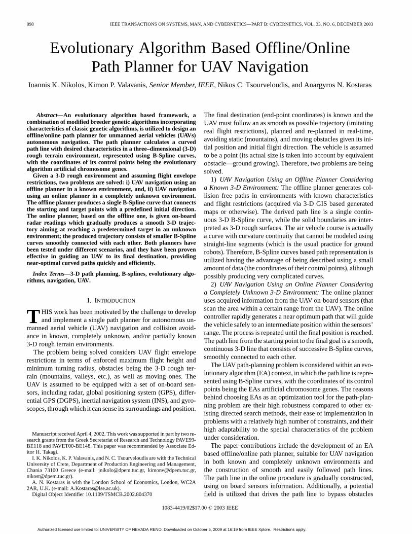
Fig. 1. Artificial terrain produced using (2).

being thethresholdof the procedure. Once chosen, these indi-viduals are used for the generation of a new population throughthe classic roulette wheel selection [3]. An elitist model assuresthat the best individual of each generation always survives theselection procedure and reproduces its structure in the next gen-eration.

This scheme provides high flexibility to the evolutionary al-gorithm. When threshold takes values close to 100% the schemeactually serves as a classic roulette scheme. For values ofclose to 10%, the scheme serves close to a classic truncationmodel. The increased selective pressure that is produced withlower values of focuses the search on the top individuals, butthe genetic diversity is lost and the procedure is trapped in localoptima. Such observations and several trial-and-error runs led tothe selection of values of between 40% and 70% in this work.

A. Solid Boundary Representation

The solid terrain under the UAV is most generally representedby a meshed 3-D surface, produced using mathematical func-tions of the form

(2)

where , , , , , , are constants experimentally defined,in order to produce a surface simulating a rough terrain withmountains and valleys (as shown in Fig. 1).

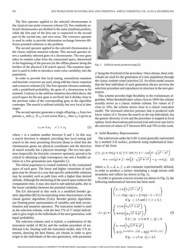
In order to generate concave terrains (as shown in Fig. 2), thefollowing mathematical function has been used:

if and

if or

if or

(3)



Fig. 2. Artificial terrain produced using (3).

where , , , , , , , , , are again proper constants,experimentally defined.

A graphical interface has been developed for the visualiza-tion of the terrain surface, along with the path line curve as in[9]. The corresponding interface deals with different terrains,produced either artificially or based on real geographical data,and provides an easy verification of the feasibility and qualityof each solution. Horizontal sections of the surface in differentheights may be plotted, visualizing the boundaries in the UAVflight height (as presented in Fig. 6). The path-planning algo-rithm considers the scanned surface as a group of quadraticmesh nodes with known coordinates. The same solid boundaryrepresentation is used for both the online and the offline method.

B. Path Line B-Spline Modeling

Straight-line segments cannot represent a flying object pathline, as usually the case with mobile robots, sea, and underseavessels. B-Splines are adopted to define the UAV desired path,providing at least first order derivative continuity. B-Splinecurves are well fitted in the evolutionary procedure, as theyneed a few variables (coordinates of the control points) in orderto define complicated curved paths (see Appendix B). Eachcontrol point has a very local effect on the curve’s shape, andsmall perturbations in its position produce changes in the curveonly in the neighborhood of the changing control point [11],[12].

A valuable characteristic of the adopted B-Spline curves isthat the curve is tangential to the control polygon at the startingand ending points. This characteristic can be used in order todefine the starting direction of the curve, by inserting an extrafixed point after the starting one. These two points can definethe direction of the curve at the corresponding region. This isessential for the path planning of flying vessels, as their flightangles are continuously defined. Consequently the direction ofthe designed path line in the starting position must coincide withthe current direction of flight in this position, in order to ensurecurvature continuity of the whole path line. The B-Spline curveis discretized, using a constant step, and it is used in this formfor the calculation of its fitness.

III. OFFLINE PATH PLANNING

The offline path planner generates a B-Spline curve overknown, simulated or real, environments. The starting and

ending points of the curve are fixed. A third point close tothe starting one is also fixed, determining the initial flightdirection. Between the fixed control points, free-to-movecontrol points determine the shape of the curve, taking values inthe constrained space. The number of the free-to-move controlpoints is fixed (user-defined). Their physical coordinates arethe genes of the EA artificial chromosome, resulting in a fixedlength chromosome.

A. Fitness Function

The optimization problem to be solved minimizes a set offour terms, connected to various constraints. The constraints areassociated with the feasibility and the length of the path line, asafety distance from the obstacles and the UAVs flight enveloperestrictions. The fitness function is the inverse of the weightedsum of the four different terms

(4)

where are weights and are the above mentioned terms de-fined as follows:

Term penalizes the nonfeasible curves that pass throughthe solid boundary. The penalty value is proportional to thenumber of discretized curve points (not the B-Spline controlpoints) located inside the solid boundary. In this way nonfea-sible curves with fewer points inside the solid boundary showbetter fitness than curves with more points inside the solidboundary. Additionally, the fitter of the nonfeasible curvesmay survive the selection procedure and produce acceptableoffsprings through the heuristic crossover operation.

Term is the length of the curve (nondimensional with thedistance between the starting and destination points) used toprovide shorter paths.

Term is designed to provide flight paths with a safety dis-tance from solid boundaries, given as

(5)

where is the number of discrete curve points,is the number of discrete mesh points of the solid boundary,

is the distance between the corresponding nodes and curvepoints, while is the minimum safety distance from thesolid boundary.

Term is designed to provide curves with a prescribedminimum curvature radius. This characteristic is essential fora flying vessel, as its flight envelope determines the minimumradius of curvature. The angle(Fig. 3) that is determined bytwo successive discrete segments of the curve (defined by thedots in Fig. 3) is calculated and if less than a prescribed value,a penalty is added to the fourth term of the fitness function.

Weights are experimentally determined, using as criterionthe almost uniform effect of the last three terms in the fitnessvalue. Term has a dominant role in (4) providing feasiblecurves in few generations, since path feasibility is the main con-cern.



Fig. 3. Schematic representation of the curvature angle used for the calculationof termf .

The maximization of Eq. (4), through the EA procedure, re-sults in a set of B-Spline control points, which actually representthe desired path.

B. Offline Procedure

Initially, the starting and ending points are externally de-termined, along with the direction of flight. The limits of thephysical space, where the vehicle is allowed to fly (, , ,upper and lower coordinates), are also determined, along withthe ground surface (in (2) or (3), or real GIS data). The givenflight direction is used to determine the third fixed point closeto the starting one. Its position is along the flight direction andat a pre-fixed distance from the starting point.

The EA randomly produces a number of chromosomes,equal to the (fixed) population number. The genes of eachchromosome are the physical coordinates of the free-to-moveB-Spline control points. These coordinates take (random)values within the limits of the constrained physical 3-Dspace. Each B-Spline curve is constructed by the three fixedcontrol points and the free-to-move ones (provided by thecorresponding chromosome).

Each B-Spline is evaluated, using the aforementioned criteria,and its fitness function is calculated. The EA proceeds, as de-scribed in Section II.

IV. ONLINE PATH PLANNING

The EA used by the online path planner is based on the oneused by the offline path planner. The main modifications con-cern the representation of the individuals, the initial population,the optimization criteria, and the gradual segment generation ofthe complete path line. The terrain is considered unknown, andonly an area near the UAV is supposed to be scanned by the onboard sensors.

A. Representation of the Individual

As the terrain is completely unknown and the radar graduallyscans the area, it is impossible to generate a feasible path that

connects the starting point with the ending one. Instead, at cer-tain moments, the radar scans a region around the UAV, and apath line is generated that connects a temporary starting pointwith a temporary ending point. Each temporary ending point isalso the next curve starting point. Therefore, what is finally gen-erated is a group of smooth curve segments, connected to eachother and eventually, connecting the starting point with the finaldestination.

In the online problem, only four control points define eachB-Spline curve, the first two of which are fixed, determining thedirection of the current UAV path. The remaining two controlpoints are allowed to take any position within the scanned by theradar known space, taking into consideration given restrictions.Only the Cartesian coordinates of the nonfixed control pointsform each individual’s genes.

When the next path segment is to be generated, only the firstcontrol point of the B-Spline curve is known, as it is the samewith the last control point of the previous B-Spline segment. Thesecond control point is not random, as it is used to make surethat at least first derivative continuity of two connected curves isprovided at the point that the two curves are connected. Hence,the second control point of the next curve should lie on the linedefined by the last two control points of the previous curve. Itis also desirable that the second control point is near the firstone, so that the UAV may easily avoid any obstacle suddenlysensed in front of it. This may happen because the radar scansthe environment not continuously, but at intervals.

B. Initial Population

A random number generator is used to produce floating-pointvalues within certain boundaries. Lower and upper boundariesform the ground area the radar scans within which the UAV isallowed to move. The control points that are randomly generatedare acceptable only if they are within the radar’s range distancefrom the UAV. Otherwise, they are ignored and new genes arebeing generated to replace them. Thus, all individuals representcurves whose control points are within the UAVs radar range.

The initial population size is now smaller compared to the of-fline path planner one, since the online problem calls for shortercomputation times.

C. Online Mechanism

As previously mentioned, the path-planning algorithm con-siders the scanned surface as a group of quadratic mesh nodes.All ground nodes are initially considered unknown. An algo-rithm is used to distinguish between nodes visible by the radarand nodes not visible as follows: A node is not visible by theUAV if it is not within the radar’s range or if it is within theradar’s range but is hidden by a ground section that lies be-tween it and the UAV. The corresponding algorithm, simulatesthe radar and checks whether the ground nodes within the radarrange are “visible” or not and consequently “known” or not.

The radar’s data are used to produce the first path line seg-ment. As the UAV is moving along this segment and until it hastraveled about 2/3 of its length, the radar scans the surroundingarea, returning a new set of visible nodes. The online planner,then, produces a new segment, whose first point is the last pointof the previous one and whose last point lies somewhere in the



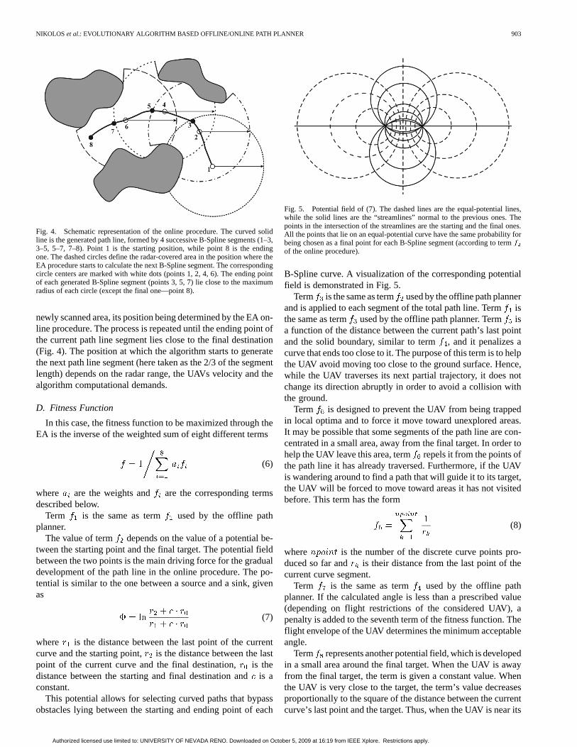
Fig. 4. Schematic representation of the online procedure. The curved solidline is the generated path line, formed by 4 successive B-Spline segments (1–3,3–5, 5–7, 7–8). Point 1 is the starting position, while point 8 is the endingone. The dashed circles define the radar-covered area in the position where theEA procedure starts to calculate the next B-Spline segment. The correspondingcircle centers are marked with white dots (points 1, 2, 4, 6). The ending pointof each generated B-Spline segment (points 3, 5, 7) lie close to the maximumradius of each circle (except the final one—point 8).

newly scanned area, its position being determined by the EA on-line procedure. The process is repeated until the ending point ofthe current path line segment lies close to the final destination(Fig. 4). The position at which the algorithm starts to generatethe next path line segment (here taken as the 2/3 of the segmentlength) depends on the radar range, the UAVs velocity and thealgorithm computational demands.

D. Fitness Function

In this case, the fitness function to be maximized through theEA is the inverse of the weighted sum of eight different terms

(6)

where are the weights and are the corresponding termsdescribed below.

Term is the same as term used by the offline pathplanner.

The value of term depends on the value of a potential be-tween the starting point and the final target. The potential fieldbetween the two points is the main driving force for the gradualdevelopment of the path line in the online procedure. The po-tential is similar to the one between a source and a sink, givenas

(7)

where is the distance between the last point of the currentcurve and the starting point, is the distance between the lastpoint of the current curve and the final destination,is thedistance between the starting and final destination andis aconstant.

This potential allows for selecting curved paths that bypassobstacles lying between the starting and ending point of each

Fig. 5. Potential field of (7). The dashed lines are the equal-potential lines,while the solid lines are the “streamlines” normal to the previous ones. Thepoints in the intersection of the streamlines are the starting and the final ones.All the points that lie on an equal-potential curve have the same probability forbeing chosen as a final point for each B-Spline segment (according to termf

of the online procedure).

B-Spline curve. A visualization of the corresponding potentialfield is demonstrated in Fig. 5.

Term is the same as term used by the offline path plannerand is applied to each segment of the total path line. Termisthe same as term used by the offline path planner. Termisa function of the distance between the current path’s last pointand the solid boundary, similar to term, and it penalizes acurve that ends too close to it. The purpose of this term is to helpthe UAV avoid moving too close to the ground surface. Hence,while the UAV traverses its next partial trajectory, it does notchange its direction abruptly in order to avoid a collision withthe ground.

Term is designed to prevent the UAV from being trappedin local optima and to force it move toward unexplored areas.It may be possible that some segments of the path line are con-centrated in a small area, away from the final target. In order tohelp the UAV leave this area, term repels it from the points ofthe path line it has already traversed. Furthermore, if the UAVis wandering around to find a path that will guide it to its target,the UAV will be forced to move toward areas it has not visitedbefore. This term has the form

(8)

where is the number of the discrete curve points pro-duced so far and is their distance from the last point of thecurrent curve segment.

Term is the same as term used by the offline pathplanner. If the calculated angle is less than a prescribed value(depending on flight restrictions of the considered UAV), apenalty is added to the seventh term of the fitness function. Theflight envelope of the UAV determines the minimum acceptableangle.

Term represents another potential field, which is developedin a small area around the final target. When the UAV is awayfrom the final target, the term is given a constant value. Whenthe UAV is very close to the target, the term’s value decreasesproportionally to the square of the distance between the currentcurve’s last point and the target. Thus, when the UAV is near its



target, the value of this term is quite small and prevents the UAVfrom moving away.

Weights are experimentally determined, using as criterionthe almost uniform effect of all the terms, except the first one.Term has a dominant role, in order to provide feasiblecurve segments in a few generations, since path feasibility isthe main concern.

E. Local Optima Avoidance Mode of the Online Path Planner

Although term has been introduced in the fitness functionof the online procedure, the ground formation may cause theUAV to be trapped in a local optimum area (consider a moun-tain with a horseshoe shape as in Fig. 2 and that the UAV entersinside its concave part, while it is not possible to overpass themountain). In such cases, it is difficult for the UAV to escapefrom this area as it would have to move away from the obstacleand thus away from its final target. To prevent this from hap-pening, a second fitness function and an algorithm is derived topredict when the UAV is about to be trapped in a local optimumand use a second mode of the online planner to overcome it.

As already stated, every time a new segment is generated, andthe radar has scanned its environment, it checks whether thereis an “obstacle” very close (within a predefined safety distance)to the UAV and toward its motion direction. An “obstacle” isa group of ground nodes higher than the flight altitude that theUAV cannot overpass, due to the constrained space in which itis allowed to move. As term has been added to the fitnessfunction, (6), which does not allow the UAV to come too closeto the ground. It is reasonable to believe that the UAV will cometoo close to the ground only if it is trapped in a local optimumarea. In addition, it is being checked whether there is an obstacleclose to the UAV, and on its way to the final destination. If noobstacle is found, the fitness function, given by (6), guides theUAV.

The goal of the second mode of the algorithm is to force theUAV to move along the border of the obstacle that has causedthe UAV to be trapped, until that obstacle lies no longer betweenthe UAV and its final destination. This is achieved by identifyingthe obstacle that has caused the UAV to be trapped. An algo-rithm, presented in Appendix A, generates a map of all groups ofnodes that form obstacles that are visible by the radar. Each suchgroup of nodes contains nodes that lie adjacent to each other.After this procedure terminates, each group of nodes has beengiven a unique number. All the nodes of a group have been giventhe same number. As the coordinates of the node that lies onthe UAVs motion direction have been stored, it is known whichgroup of nodes (obstacle) has caused the UAV to be trapped inthe local optimum area (see Appendix A).

Next, the borders (the corresponding nodes) of the obstacleare located and assigned a numerical value, so that the nodewith the greater value is far from the UAVs current position.The second fitness function forces the UAV to move along theborder and toward the border node with the larger value.

When the UAV reaches its new position, the whole processgoes over again (in the same mode) and the UAV keeps movingacross the obstacle’s borders, (momentarily) ignoring its finaldestination. The algorithm returns to the first mode when theobstacle is no longer between the UAV and the final destination.

F. Second Fitness Function of the Online Procedure

The second fitness function is used within the local optimaavoidance mode of the online procedure, when the UAV istrapped in a local optimum.

It is the inverse of the weighted sum of three different terms

(9)

where are the weights and are the corresponding termsdescribed below. Term is the same as the term used by theoffline path planner. The value of term penalizes curves whentheir last point is far from the border node whose identificationnumber was given the greater value. This term is used to enforcethe curve to circle the obstacle.

Term is the nondimensional length of the current curve,used in order to provide short and smooth paths. Weightsareexperimentally determined. Term has a dominant role, inorder to provide feasible curves in a few generations, since pathfeasibility is the main concern.

The second fitness function works in a different way thanterm of the first fitness function. Term repels the UAVfrom the points of the path line it has already traversed, in orderto explore new areas, and avoid “going around” in the local op-timum area. The second fitness function forces the path line tomove along the border of the obstacle that has caused the UAVto be trapped, until that obstacle no longer lies between the UAVand its final destination.

This second fitness function is used to generate a new pathline segment if the UAV has been trapped in a local optimumarea. After the calculation of the new path line segment, usingthe second fitness function, the UAV moves along this segment,until it reaches the 2/3 of segment’s length. If the obstacle isno longer between the current UAV position and its final des-tination, the algorithm returns to the first mode of the onlineprocedure, and the fitness function defined in (6) is used. If theobstacle is still between the UAV and the final destination, thenext path line segment will be generated with the fitness func-tion defined in (9) (the second one), within the second mode ofthe online procedure.

V. EXPERIMENTAL RESULTS

A. Offline Experiments

The offline planner has been extensively tested, using a sim-ulation environment. All experiments have been designed inorder to search for path lines between “mountains.” For thisreason, an upper ceiling for flight height has been enforced. Thisceiling is represented in the graphical environment by the hori-zontal section of the terrain (Fig. 6).

The (experimentally optimized) settings of the evolutionaryalgorithm for the offline planner are as follows:population size

100,threshold 0.5,heuristic crossover probability 0.75,classic crossover probability 0.25,classic mutation proba-bility 0.05,nonuniform mutation probability 0.13. The de-tailed procedure of the parameter selection is presented in Ap-pendix C.



Fig. 6. First offline test case: Four free-to-move control points were used, witha prefixed direction at the starting position. The starting position is marked witha circle.

Fig. 7. Second offline test case.

The algorithm was defined to terminate after 50 generations,although feasible solutions can be reached in less than 10 itera-tions. With 50 generations, and a population size equal to 100,5000 evaluations of the fitness function are performed before thealgorithm stops. The calculation corresponds to 15 s computa-tion time per generation, in a 700 MHz PC, for a chromosomelength equal to 12 (4 free-to-move control points), and a terraindescribed with 53 53 nodes.

In the offline test cases presented here, the free-to-move con-trol points were taking values between 4–6, resulting in a totalnumber of B-Spline control points equal to 7–9 (along with thefixed starting and target points, and the fixed second point, usedfor the determination of the initial direction). Greater number ofcontrol points resulted in higher computation time and slowerconvergence rate, without any significant profit, concerning thefitness of the curve.

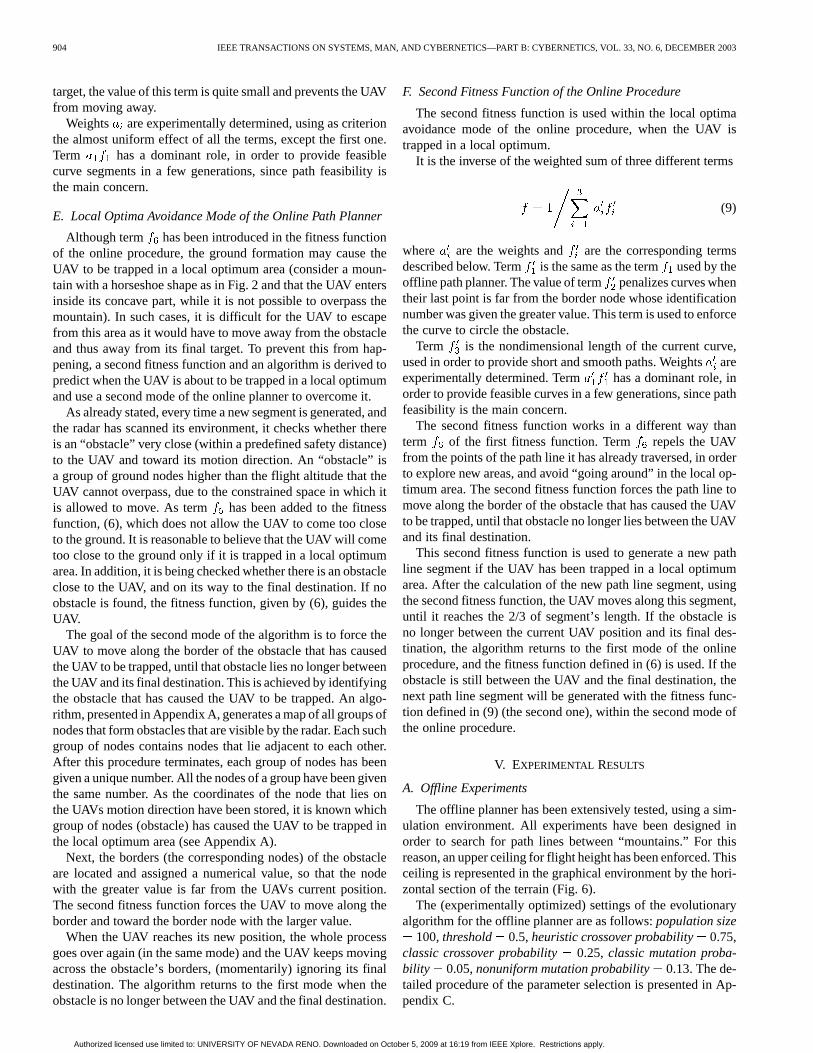
The test cases shown in Figs. 10 and 11 were designed withthe ceiling set to a low altitude which increased the path plan-ning difficulty. The minimum distance from the mountain-likeboundaries was empirically set equal to 1/30 of the-dimen-sion of the terrain, in all the cases, except for case 3, which ispresented in Figs. 8 and 9. In test case 3, the minimum distance

Fig. 8. Third offline test case.

Fig. 9. Early feasible solution of the third offline test case.

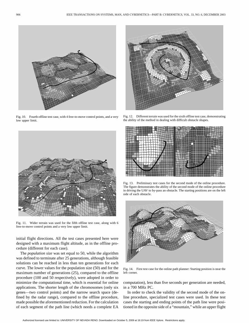
was set equal to the 1/15 of the terrain’s-dimension. As it isdemonstrated in Fig. 8, a higher distance from the solid bound-aries was achieved, compared to test case 2 (Fig. 7). For the testcase 5, shown in Fig. 11, a wider terrain was used. For the testcase 6, shown in Fig. 12, a horseshoe terrain was used [producedwith (3)], demonstrating the ability of the method to deal withU-shaped obstacles.

Relatively high values of mutation probabilities wereadopted, in order to ensure the ability of the algorithm to over-come local optima. As it was observed, initial feasible solutionsprovided by the evolutionary algorithm, were progressivelyreplaced by fitter ones, with a completely different structure.Figs. 8 and 9 demonstrate the above observation.

B. Online Experiments

The same environment was used for all the test cases consid-ered, with different starting and destination points and different



Fig. 10. Fourth offline test case, with 4 free-to-move control points, and a verylow upper limit.

Fig. 11. Wider terrain was used for the fifth offline test case, along with 6free-to-move control points and a very low upper limit.

initial flight directions. All the test cases presented here weredesigned with a maximum flight altitude, as in the offline pro-cedure (different for each case).

Thepopulation sizewas set equal to 50, while the algorithmwas defined to terminate after 25 generations, although feasiblesolutions can be reached in less than ten generations for eachcurve. The lower values for the population size (50) and for themaximum number of generations (25), compared to the offlineprocedure (100 and 50 respectively), were adopted in order tominimize the computational time, which is essential for onlineapplications. The shorter length of the chromosomes (only sixgenes—two control points) and the narrow search space (de-fined by the radar range), compared to the offline procedure,made possible the aforementioned reduction. For the calculationof each segment of the path line (which needs a complete EA

Fig. 12. Different terrain was used for the sixth offline test case, demonstratingthe ability of the method in dealing with difficult obstacle shapes.

Fig. 13. Preliminary test cases for the second mode of the online procedure.The figure demonstrates the ability of the second mode of the online procedurein driving the UAV to by-pass an obstacle. The starting positions are on the leftside of each obstacle.

Fig. 14. First test case for the online path planner: Starting position is near theleft corner.

computation), less than five seconds per generation are needed,in a 700 MHz PC.

In order to check the validity of the second mode of the on-line procedure, specialized test cases were used. In these testcases the starting and ending points of the path line were posi-tioned in the opposite side of a “mountain,” while an upper flight



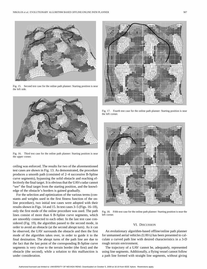
Fig. 15. Second test case for the online path planner: Starting position is nearthe left side.

Fig. 16. Third test case for the online path planner: Starting position is nearthe upper corner.

ceiling was enforced. The results for two of the aforementionedtest cases are shown in Fig. 13. As demonstrated, the procedureproduces a smooth path (consisted of 2–4 successive B-Splinecurve segments), bypassing the solid obstacle and reaching ef-fectively the final target. It is obvious that the UAVs radar cannot“see” the final target from the starting position, and the knowl-edge of the obstacle’s borders is gained gradually.

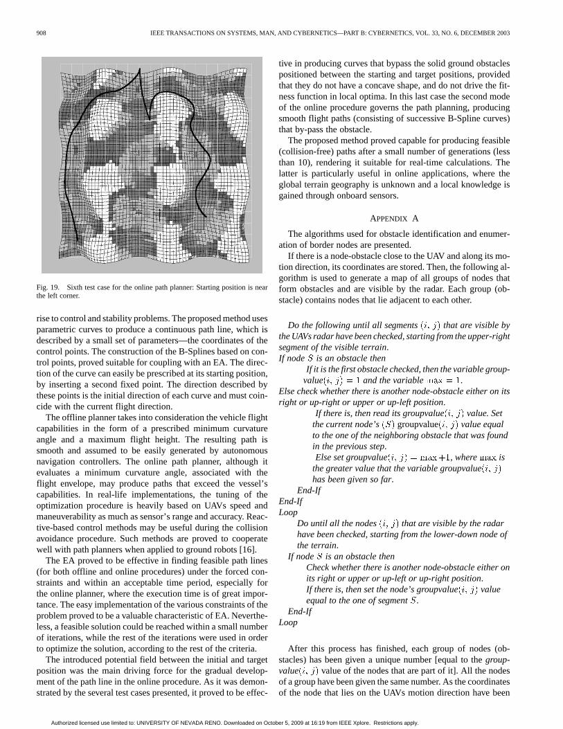
For the selection and optimization of the various terms (con-stants and weights used in the first fitness function of the on-line procedure), two initial test cases were adopted with theirresults shown in Figs. 14 and 15. In test cases 3–5 (Figs. 16–18),only the first mode of the online procedure was used. The pathlines consist of more than 6 B-Spline curve segments, whichare smoothly connected to each other. In the last test case con-sidered (Fig. 19), the algorithm passed to the second mode, inorder to avoid an obstacle (at the second abrupt turn). As it canbe observed, the UAV surrounds the obstacle and then the firstmode of the algorithm takes over, in order to guide it to thefinal destination. The abrupt turns of the path line are due tothe fact that the last point of the corresponding B-Spline curvesegments is very close to the terrain border (the first) and theobstacle (the second), while a solution to this malfunction isunder consideration.

Fig. 17. Fourth test case for the online path planner: Starting position is nearthe left corner.

Fig. 18. Fifth test case for the online path planner: Starting position is near theleft corner.

VI. DISCUSSION

An evolutionary algorithm-based offline/online path plannerfor unmanned aerial vehicles (UAVs) has been presented to cal-culate a curved path line with desired characteristics in a 3-Drough terrain environment.

The trajectory of a UAV cannot be, adequately, representedusing line segments. Additionally, a flying vessel cannot followa path line formed with straight line segments, without giving



Fig. 19. Sixth test case for the online path planner: Starting position is nearthe left corner.

rise to control and stability problems. The proposed method usesparametric curves to produce a continuous path line, which isdescribed by a small set of parameters—the coordinates of thecontrol points. The construction of the B-Splines based on con-trol points, proved suitable for coupling with an EA. The direc-tion of the curve can easily be prescribed at its starting position,by inserting a second fixed point. The direction described bythese points is the initial direction of each curve and must coin-cide with the current flight direction.

The offline planner takes into consideration the vehicle flightcapabilities in the form of a prescribed minimum curvatureangle and a maximum flight height. The resulting path issmooth and assumed to be easily generated by autonomousnavigation controllers. The online path planner, although itevaluates a minimum curvature angle, associated with theflight envelope, may produce paths that exceed the vessel’scapabilities. In real-life implementations, the tuning of theoptimization procedure is heavily based on UAVs speed andmaneuverability as much as sensor’s range and accuracy. Reac-tive-based control methods may be useful during the collisionavoidance procedure. Such methods are proved to cooperatewell with path planners when applied to ground robots [16].

The EA proved to be effective in finding feasible path lines(for both offline and online procedures) under the forced con-straints and within an acceptable time period, especially forthe online planner, where the execution time is of great impor-tance. The easy implementation of the various constraints of theproblem proved to be a valuable characteristic of EA. Neverthe-less, a feasible solution could be reached within a small numberof iterations, while the rest of the iterations were used in orderto optimize the solution, according to the rest of the criteria.

The introduced potential field between the initial and targetposition was the main driving force for the gradual develop-ment of the path line in the online procedure. As it was demon-strated by the several test cases presented, it proved to be effec-

tive in producing curves that bypass the solid ground obstaclespositioned between the starting and target positions, providedthat they do not have a concave shape, and do not drive the fit-ness function in local optima. In this last case the second modeof the online procedure governs the path planning, producingsmooth flight paths (consisting of successive B-Spline curves)that by-pass the obstacle.

The proposed method proved capable for producing feasible(collision-free) paths after a small number of generations (lessthan 10), rendering it suitable for real-time calculations. Thelatter is particularly useful in online applications, where theglobal terrain geography is unknown and a local knowledge isgained through onboard sensors.

APPENDIX A

The algorithms used for obstacle identification and enumer-ation of border nodes are presented.

If there is a node-obstacle close to the UAV and along its mo-tion direction, its coordinates are stored. Then, the following al-gorithm is used to generate a map of all groups of nodes thatform obstacles and are visible by the radar. Each group (ob-stacle) contains nodes that lie adjacent to each other.

Do the following until all segments that are visible bythe UAVs radar have been checked, starting from the upper-rightsegment of the visible terrain.If node is an obstacle then

If it is the first obstacle checked, then the variable group-value and the variable .

Else check whether there is another node-obstacle either on itsright or up-right or upper or up-left position.

If there is, then read its groupvalue value. Setthe current node’s groupvalue value equalto the one of the neighboring obstacle that was foundin the previous step.Else set groupvalue , where is

the greater value that the variable groupvaluehas been given so far.

End-IfEnd-IfLoop

Do until all the nodes that are visible by the radarhave been checked, starting from the lower-down node ofthe terrain.

If node is an obstacle thenCheck whether there is another node-obstacle either onits right or upper or up-left or up-right position.If there is, then set the node’s groupvalue valueequal to the one of segment.

End-IfLoop

After this process has finished, each group of nodes (ob-stacles) has been given a unique number [equal to thegroup-value value of the nodes that are part of it]. All the nodesof a group have been given the same number. As the coordinatesof the node that lies on the UAVs motion direction have been



kept, it is known which group of nodes (obstacle) has causedthe UAV to be trapped in a local optimum area.

Next, the obstacle’s borders are located and are enumeratedso that the node with the greater number is far from the UAVscurrent position. The following algorithm is used in order toenumerate the nodes of the obstacle that are part of its border.

A. Counter-Clockwise Numeration

Give the value 0 to the variable num for the obstacle that lieson the UAVs motion direction and whose coordinates have beenalready stored.Check whether there is another border-nodeof the group ofobstacles in the 8 surrounding positions, using counter clock-wise direction and starting from the lower position.If there is, then the variable is given the value

and the same process is repeated for the new node. The process is repeated until there is no other border-node

adjacent to the current node for which the variable num hasnot been given a value.

If the current node lies on the border of the terrain, thenclockwise numeration is needed, so as the UAV not to moveoutside the terrain.

B. Clockwise Numeration

Give the value 0 to the variable num for the obstacle that lieson the UAVs motion direction and whose coordinates have beenalready kept.Check whether there is another segment-borderof the groupof obstacles, in the 8 surrounding positions, using clockwise di-rection and starting from the upper position.If there is, then the variable is given the value

and the same process is repeated for the new segment. The process is repeated until there is no other segment-border

adjacent to the current segmentfor which the variable numhas not been given a value.

APPENDIX B

B-Spline curves are parametric curves, with their con-struction based on blending functions [11], [12]. Theirparametric construction provides the ability to producenonmonotonic curves. If the number of control pointsof the corresponding curve is , with coordinates

, the coordinates of theB-Spline may be written as

(10)

(11)

(12)

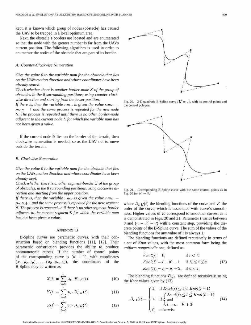
Fig. 20. 2-D quadratic B-Spline curve(K = 3), with its control points andthe control polygon.

Fig. 21. Corresponding B-Spline curve with the same control points as inFig. 20 forK = 5.

where the blending functions of the curve and theorder of the curve, which is associated with curve’s smooth-ness. Higher values of correspond to smoother curves, as itis demonstrated in Figs. 20 and 21. Parameter t varies between0 and with a constant step, providing the dis-crete points of the B-Spline curve. The sum of the values of theblending functions for any value ofis always 1.

The blending functions are defined recursively in terms ofa set ofKnot values, with the most common form being theuniform nonperiodicone, defined as:

Knot if

Knot if

Knot if

(13)

The blending functions are defined recursively, usingtheKnot values given by (13)

if Knot Knot

ifKnot Knot

and

otherwise

(14)



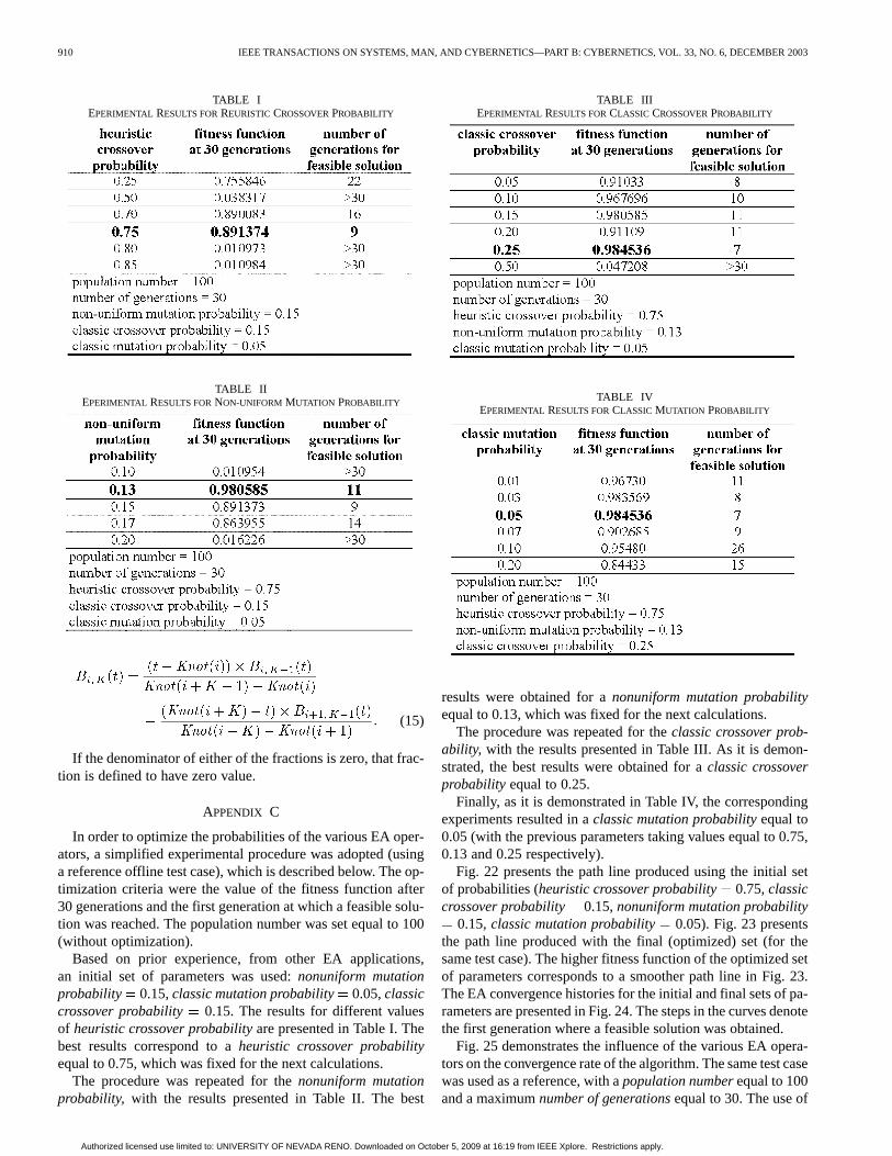
TABLE IEPERIMENTAL RESULTS FORREURISTIC CROSSOVERPROBABILITY

TABLE IIEPERIMENTAL RESULTS FORNON-UNIFORM MUTATION PROBABILITY

Knot

Knot Knot

Knot

Knot Knot(15)

If the denominator of either of the fractions is zero, that frac-tion is defined to have zero value.

APPENDIX C

In order to optimize the probabilities of the various EA oper-ators, a simplified experimental procedure was adopted (usinga reference offline test case), which is described below. The op-timization criteria were the value of the fitness function after30 generations and the first generation at which a feasible solu-tion was reached. The population number was set equal to 100(without optimization).

Based on prior experience, from other EA applications,an initial set of parameters was used:nonuniform mutationprobability 0.15,classic mutation probability 0.05,classiccrossover probability 0.15. The results for different valuesof heuristic crossover probabilityare presented in Table I. Thebest results correspond to aheuristic crossover probabilityequal to 0.75, which was fixed for the next calculations.

The procedure was repeated for thenonuniform mutationprobability, with the results presented in Table II. The best

TABLE IIIEPERIMENTAL RESULTS FORCLASSIC CROSSOVERPROBABILITY

TABLE IVEPERIMENTAL RESULTS FORCLASSIC MUTATION PROBABILITY

results were obtained for anonuniform mutation probabilityequal to 0.13, which was fixed for the next calculations.

The procedure was repeated for theclassic crossover prob-ability, with the results presented in Table III. As it is demon-strated, the best results were obtained for aclassic crossoverprobability equal to 0.25.

Finally, as it is demonstrated in Table IV, the correspondingexperiments resulted in aclassic mutation probabilityequal to0.05 (with the previous parameters taking values equal to 0.75,0.13 and 0.25 respectively).

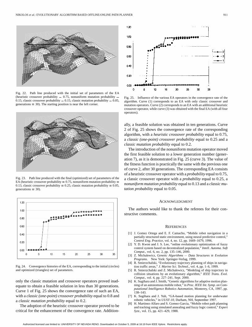
Fig. 22 presents the path line produced using the initial setof probabilities (heuristic crossover probability 0.75,classiccrossover probability 0.15,nonuniform mutation probability

0.15,classic mutation probability 0.05). Fig. 23 presentsthe path line produced with the final (optimized) set (for thesame test case). The higher fitness function of the optimized setof parameters corresponds to a smoother path line in Fig. 23.The EA convergence histories for the initial and final sets of pa-rameters are presented in Fig. 24. The steps in the curves denotethe first generation where a feasible solution was obtained.

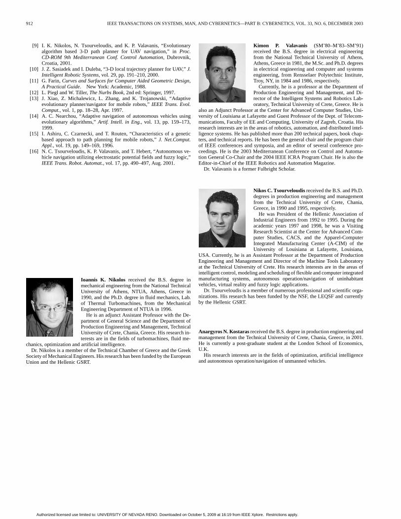
Fig. 25 demonstrates the influence of the various EA opera-tors on the convergence rate of the algorithm. The same test casewas used as a reference, with apopulation numberequal to 100and a maximumnumber of generationsequal to 30. The use of



Fig. 22. Path line produced with the initial set of parameters of the EA(heuristic crossover probability= 0.75, nonuniform mutation probability=0.15, classic crossover probability= 0.15, classic mutation probability= 0.05,generations= 30). The starting position is near the left corner.

Fig. 23. Path line produced with the final (optimized) set of parameters of theEA (heuristic crossover probability= 0.75, nonuniform mutation probability=0.13, classic crossover probability= 0.25, classic mutation probability= 0.05,generations= 30).

Fig. 24. Convergence histories of the EA, corresponding to the initial (circles)and optimized (triangles) set of parameters.

only the classic mutation and crossover operators proved inad-equate to obtain a feasible solution in less than 30 generations.Curve 1 of Fig. 25 shows the convergence rate of such an EA,with aclassic (one-point) crossover probabilityequal to 0.8 anda classic mutation probabilityequal to 0.2.

The adoption of the heuristic crossover operator proved to becritical for the enhancement of the convergence rate. Addition-

Fig. 25. Influence of the various EA operators in the convergence rate of thealgorithm. Curve (1) corresponds to an EA with only classic crossover andmutation operators. Curve (2) corresponds to an EA with an additional heuristiccrossover operator, while curve (3) was obtained with the final EA (with all fouroperators).

ally, a feasible solution was obtained in ten generations. Curve2 of Fig. 25 shows the convergence rate of the correspondingalgorithm, with aheuristic crossover probabilityequal to 0.75,a classic (one-point) crossover probabilityequal to 0.25 and aclassic mutation probabilityequal to 0.2.

The introduction of the nonuniform mutation operator movedthe first feasible solution to a lower generation number (gener-ation 7), as it is demonstrated in Fig. 25 (curve 3). The value ofthe fitness function is practically the same with the previous oneof curve 2, after 30 generations. The corresponding EA consistsof a heuristic crossover operator with aprobabilityequal to 0.75,a classic crossover operator with aprobability equal to 0.25, anonuniform mutation probabilityequal to 0.13 and aclassic mu-tation probabilityequal to 0.05.

ACKNOWLEDGMENT

The authors would like to thank the referees for their con-structive comments.

REFERENCES

[1] J. Gomez Ortega and E. F. Camacho, “Mobile robot navigation in apartially structured static environment, using neural predictive control,”Control Eng. Practice, vol. 4, no. 12, pp. 1669–1679, 1996.

[2] Y. D. Kwon and J. S. Lee, “online evolutionary optimization of fuzzycontrol system based on decentralized population,”Intell. Automa. SoftComput., vol. 6, no. 2, pp. 135–146, 2000.

[3] Z. Michalewicz, Genetic Algorithms+ Data Structures= EvolutionPrograms. New York: Springer-Verlag, 1999.

[4] R. Smierzchalski, “Evolutionary trajectory planning of ships in naviga-tion traffic areas,”J. Marine Sci. Technol., vol. 4, pp. 1–6, 1999.

[5] R. Smierzchalski and Z. Michalewicz, “Modeling of ship trajectory incollision situations by an evolutionary algorithm,”IEEE Trans. Evol.Comput., vol. 4, pp. 227–241, Sept. 2000.

[6] K. Sugihara and J. Smith, “Genetic algorithms for adaptive motion plan-ning of an autonomous mobile robot,” inProc. IEEE Int. Symp. on Com-putational Intelligence Robotics Automation, Monterey, CA, 1997, pp.138–143.

[7] K. Sugihara and J. Yuh, “GA-based motion planning for underwaterrobotic vehicles,” inUUST-10, Durham, NH, September 1997.

[8] H. Martinez-Alfaro and S. Gomez-Garcia, “Mobile robot path planningand tracking using simulated annealing and fuzzy logic control,”ExpertSyst., vol. 15, pp. 421–429, 1988.



[9] I. K. Nikolos, N. Tsourveloudis, and K. P. Valavanis, “Evolutionaryalgorithm based 3-D path planner for UAV navigation,” inProc.CD-ROM 9th Mediterranean Conf. Control Automation, Dubrovnik,Croatia, 2001.

[10] J. Z. Sasiadek and I. Duleba, “3-D local trajectory planner for UAV,”J.Intelligent Robotic Systems, vol. 29, pp. 191–210, 2000.

[11] G. Farin,Curves and Surfaces for Computer Aided Geometric Design,A Practical Guide. New York: Academic, 1988.

[12] L. Piegl and W. Tiller,The Nurbs Book, 2nd ed: Springer, 1997.[13] J. Xiao, Z. Michalewicz, L. Zhang, and K. Trojanowski, “Adaptive

evolutionary planner/navigator for mobile robots,”IEEE Trans. Evol.Comput., vol. 1, pp. 18–28, Apr. 1997.

[14] A. C. Nearchou, “Adaptive navigation of autonomous vehicles usingevolutionary algorithms,”Artif. Intell. in Eng., vol. 13, pp. 159–173,1999.

[15] I. Ashiru, C. Czarnecki, and T. Routen, “Characteristics of a geneticbased approach to path planning for mobile robots,”J. Net.Comput.Appl., vol. 19, pp. 149–169, 1996.

[16] N. C. Tsourveloudis, K. P. Valavanis, and T. Hebert, “Autonomous ve-hicle navigation utilizing electrostatic potential fields and fuzzy logic,”IEEE Trans. Robot. Automat., vol. 17, pp. 490–497, Aug. 2001.

Ioannis K. Nikolos received the B.S. degree inmechanical engineering from the National TechnicalUniversity of Athens, NTUA, Athens, Greece in1990, and the Ph.D. degree in fluid mechanics, Lab.of Thermal Turbomachines, from the MechanicalEngineering Department of NTUA in 1996.

He is an adjunct Assistant Professor with the De-partment of General Science and the Department ofProduction Engineering and Management, TechnicalUniversity of Crete, Chania, Greece. His research in-terests are in the fields of turbomachines, fluid me-

chanics, optimization and artificial intelligence.Dr. Nikolos is a member of the Technical Chamber of Greece and the Greek

Society of Mechanical Engineers. His research has been funded by the EuropeanUnion and the Hellenic GSRT.

Kimon P. Valavanis (SM’80–M’83–SM’91)received the B.S. degree in electrical engineeringfrom the National Technical University of Athens,Athens, Greece in 1981, the M.Sc. and Ph.D. degreesin electrical engineering and computer and systemsengineering, from Rensselaer Polytechnic Institute,Troy, NY, in 1984 and 1986, respectively.

Currently, he is a professor at the Department ofProduction Engineering and Management, and Di-rector of the Intelligent Systems and Robotics Lab-oratory, Technical University of Crete, Greece. He is

also an Adjunct Professor at the Center for Advanced Computer Studies, Uni-versity of Louisiana at Lafayette and Guest Professor of the Dept. of Telecom-munications, Faculty of EE and Computing, University of Zagreb, Croatia. Hisresearch interests are in the areas of robotics, automation, and distributed intel-ligence systems. He has published more than 200 technical papers, book chap-ters, and technical reports. He has been the general chair and the program chairof IEEE conferences and symposia, and an editor of several conference pro-ceedings. He is the 2003 Mediterranean Conference on Control and Automa-tion General Co-Chair and the 2004 IEEE ICRA Program Chair. He is also theEditor-in-Chief of the IEEE Robotics and Automation Magazine.

Dr. Valavanis is a former Fulbright Scholar.

Nikos C. Tsourveloudisreceived the B.S. and Ph.D.degrees in production engineering and managementfrom the Technical University of Crete, Chania,Greece, in 1990 and 1995, respectively.

He was President of the Hellenic Association ofIndustrial Engineers from 1992 to 1995. During theacademic years 1997 and 1998, he was a VisitingResearch Scientist at the Center for Advanced Com-puter Studies, CACS, and the Apparel-ComputerIntegrated Manufacturing Center (A-CIM) of theUniversity of Louisiana at Lafayette, Louisiana,

USA. Currently, he is an Assistant Professor at the Department of ProductionEngineering and Management and Director of the Machine Tools Laboratoryat the Technical University of Crete. His research interests are in the areas ofintelligent control, modeling and scheduling of flexible and computer integratedmanufacturing systems, autonomous operation/navigation of uninhabitantvehicles, virtual reality and fuzzy logic applications.

Dr. Tsourveloudis is a member of numerous professional and scientific orga-nizations. His research has been funded by the NSF, the LEQSF and currentlyby the Hellenic GSRT.

Anargyros N. Kostarasreceived the B.S. degree in production engineering andmanagement from the Technical University of Crete, Chania, Greece, in 2001.He is currently a post-graduate student at the London School of Economics,U.K.

His research interests are in the fields of optimization, artificial intelligenceand autonomous operation/navigation of unmanned vehicles.


evolutionary algorithm based offline/online path...

Documents