evolutionary computation in continuous optimization …1107808/fulltext01.pdf · continuous...
TRANSCRIPT

Malardalen UniversitySchool of Innovation Design and Engineering
Vasteras, Sweden
Bachelor Thesis
EVOLUTIONARY COMPUTATION INCONTINUOUS OPTIMIZATION AND
MACHINE LEARNING
Leslie [email protected]
Examiner: Peter Funk
Malardalen UniversityVasteras, Sweden
Supervisor: Ning Xiong
Malardalen UniversityVasteras, Sweden
June 10, 2017

Malardalen University Leslie Dahlberg
Abstract
Evolutionary computation is a field which uses natural computational processes to optimizemathematical and industrial problems. Differential Evolution, Particle Swarm Optimization andEstimation of Distribution Algorithm are some of the newer emerging varieties which have attractedgreat interest among researchers. This work has compared these three algorithms on a set of math-ematical and machine learning benchmarks and also synthesized a new algorithm from the threeother ones and compared it to them. The results from the benchmark show which algorithm is bestsuited to handle various machine learning problems and presents the advantages of using the newalgorithm. The new algorithm called DEDA (Differential Estimation of Distribution Algorithms)has shown promising results at both machine learning and mathematical optimization tasks.
1

Malardalen University Leslie Dahlberg
Contents
1 Introduction 3
2 Background 42.1 Evolutionary Algorithms . . . . . . . . . . . . . . . . . . . . . . . . . . . . . . . . . 4
2.1.1 Representation . . . . . . . . . . . . . . . . . . . . . . . . . . . . . . . . . . 42.1.2 Evaluation function . . . . . . . . . . . . . . . . . . . . . . . . . . . . . . . 52.1.3 Population . . . . . . . . . . . . . . . . . . . . . . . . . . . . . . . . . . . . 52.1.4 Parent selection mechanism . . . . . . . . . . . . . . . . . . . . . . . . . . . 62.1.5 Variation operators . . . . . . . . . . . . . . . . . . . . . . . . . . . . . . . . 62.1.6 Survivor selection mechanism . . . . . . . . . . . . . . . . . . . . . . . . . . 72.1.7 Initialization . . . . . . . . . . . . . . . . . . . . . . . . . . . . . . . . . . . 72.1.8 Termination condition . . . . . . . . . . . . . . . . . . . . . . . . . . . . . . 7
2.2 Traditional Evolutionary Algorithms . . . . . . . . . . . . . . . . . . . . . . . . . . 72.2.1 Genetic algorithms . . . . . . . . . . . . . . . . . . . . . . . . . . . . . . . . 82.2.2 Evolution strategy . . . . . . . . . . . . . . . . . . . . . . . . . . . . . . . . 82.2.3 Evolutionary programming . . . . . . . . . . . . . . . . . . . . . . . . . . . 92.2.4 Genetic programming . . . . . . . . . . . . . . . . . . . . . . . . . . . . . . 9
2.3 Emerging Evolutionary Algorithms . . . . . . . . . . . . . . . . . . . . . . . . . . . 102.3.1 Differential Evolution . . . . . . . . . . . . . . . . . . . . . . . . . . . . . . 102.3.2 Particle Swarm Optimization . . . . . . . . . . . . . . . . . . . . . . . . . . 112.3.3 Estimation of Distribution Algorithm . . . . . . . . . . . . . . . . . . . . . 12
2.4 Machine learning concepts . . . . . . . . . . . . . . . . . . . . . . . . . . . . . . . . 122.4.1 Artificial Neuron . . . . . . . . . . . . . . . . . . . . . . . . . . . . . . . . . 132.4.2 Artificial Neural Networks . . . . . . . . . . . . . . . . . . . . . . . . . . . . 142.4.3 Back-propagation . . . . . . . . . . . . . . . . . . . . . . . . . . . . . . . . . 14
3 Related Work 163.1 Recent Research . . . . . . . . . . . . . . . . . . . . . . . . . . . . . . . . . . . . . 163.2 Emerging Evolutionary Algorithms . . . . . . . . . . . . . . . . . . . . . . . . . . . 163.3 Evolutionary Algorithms and Machine Learning . . . . . . . . . . . . . . . . . . . . 173.4 Contributions . . . . . . . . . . . . . . . . . . . . . . . . . . . . . . . . . . . . . . . 17
4 Problem Formulation 184.1 Method . . . . . . . . . . . . . . . . . . . . . . . . . . . . . . . . . . . . . . . . . . 19
5 The Proposed Algorithm 20
6 Experimental Results and Evaluation 226.1 Mathematical Function Optimization (F1−10) . . . . . . . . . . . . . . . . . . . . . 226.2 Function Approximation (FA1−6) . . . . . . . . . . . . . . . . . . . . . . . . . . . 256.3 Classification (CLS1−7) . . . . . . . . . . . . . . . . . . . . . . . . . . . . . . . . . 256.4 Clustering (CLU1) . . . . . . . . . . . . . . . . . . . . . . . . . . . . . . . . . . . . 266.5 Intelligent Game Controllers (IGC1) . . . . . . . . . . . . . . . . . . . . . . . . . . 266.6 Results . . . . . . . . . . . . . . . . . . . . . . . . . . . . . . . . . . . . . . . . . . . 296.7 Discussion . . . . . . . . . . . . . . . . . . . . . . . . . . . . . . . . . . . . . . . . . 32
7 Conclusions 337.1 Future Work . . . . . . . . . . . . . . . . . . . . . . . . . . . . . . . . . . . . . . . 33
References 36
Appendix A Algorithms 37A.1 Differential Estimation of Distribution . . . . . . . . . . . . . . . . . . . . . . . . . 37
2

Malardalen University Leslie Dahlberg
1 Introduction
Optimization is a problem-solving method which aims to find the most advantageous parametersfor a given model. The model is known to the optimizer and accepts inputs while producingoutputs. Usually the problem can be formulated in such a way that we seek to minimize theoutput value of the model or the output of some function which transforms the model’s outputinto a fitness score. Because of this the process is often referred to as minimization. It becomesobvious that this is useful when considering optimizing the layout of a circuit in order to minimizethe power consumption. To achieve this the optimizer looks for combinations of parameters whichlet the model produce the best output to a given input [1].
When dealing with simple mathematical models, optimization can be achieved using analyticalmethods, often calculating the derivative of the functional model, but these methods prove difficultto adapt to complex models which exhibit noisy behavior. Additionally, the analytical model isnot always known, which makes it impossible to use such methods [2]. The field of evolutionarycomputation (EC), a subset of computational intelligence (CI), which is further a subset of artificialintelligence (AI), contains algorithms which are well suited to solving these kinds of optimizationproblems [3, 4].
Evolutionary computation focuses on problem solving algorithms which draw inspiration fromnatural processes. It is closely related to the neighboring field of swarm intelligence (SI), whichoften is, and in this thesis will be, included as a subset of EC. The basic rationale of the fieldis to adapt the mathematical models of biological Darwinian evolution to optimization problems.The usefulness of this can be illustrated by imagining that an organism acts as an “input” to the“model” of it’s natural environment and produces an “output” in the form of offspring. Throughmultiple iterations biological evolution culls the population of organisms, only keeping the fit spec-imen, to produce organisms which become continuously better adapted to their environments.Evolutionary computation is, however, not merely confined to Darwinian evolution, but also in-cludes a multitude of methods which draw from other natural processes such as cultural evolutionand animal behavior [5].
The purpose of this thesis is to explore the performance and usefulness of three emerging evolu-tionary algorithms: differential evolution, particle swarm optimization and estimation of distribu-tion algorithms. These algorithms are newer inventions inspired by genetic algorithms, evolutionstrategy, evolutionary programming and genetic programming. Differential evolution is a straight-forward evolutionary algorithm which uses simple mathematic vector calculations to achieve it’sresults, while particle swarm optimization tries to mirror the behavior of swarming animals and es-timation of distribution uses probability distributions to guess it’s way forward. The intention is totest and compare these against each other on a set of standard mathematical benchmark functionsand practical problems in machine learning involving neural networks and game controllers andthen, if possible, develop a new or modified algorithm which improves upon the aforementionedones in some aspect.
Research has been conducted on improving various evolutionary algorithms by hybridizing andextending them, which has resulted in a wide array of algorithms for both specific and generalpurposes. Since these algorithms accept parameters which modify their efficiency, studies havebeen carried out which compare different combinations of parameters. My thesis will draw uponthis work by comparing three algorithms both generally and on a very specific problem.
The results from the benchmark show which algorithm is best suited to handle various machinelearning problems and presents the advantages of using the new algorithm. The new algorithmcalled DEDA (Differential Estimation of Distribution Algorithms) has shown promising results atboth machine learning and mathematical optimization tasks.
3

Malardalen University Leslie Dahlberg
2 Background
This section will aim to provide a general overview of the field of evolutionary computation. Generalterms and procedures which are often utilized in EC will be explained and the most well knowntraditional approaches will be presented. The necessary concepts from machine learning will bepresented.
2.1 Evolutionary Algorithms
Evolutionary algorithms work on the concept of populations. A population is a set of individualswhich in the case of optimization problems contains a vector of parameters which the model wewish to optimize can accept and transform into an output. The population is initialized by someprocedure to contain a random set of parameter vectors, these should cover the whole parameterrange of the model uniformly. The initial population is evaluated and an iterative process is startedwhich continues as long as no suitable solution is found. During this iterative process the currentpopulation is selected, altered and evaluated. During selection a set of individuals which displaypromising characteristics are selected to live on into the next generation of the population. Theyare then altered randomly to create diversity in the population and evaluated. This process createsa new generation of the population on each iteration and continues until a solution is found or someother restriction is encountered [6]. The concept is demonstrated in figure 1 with P (t) representingthe population at generation t.
Algorithm 1 Basic evolutionary algorithm
t← 0initialize P (t)evaluate P (t)while termination-condition not fulfilled do
t← t+ 1select P (t) from P (t− 1)alter P (t)evaluate P (t)
end while
Here the fundamental building-blocks of evolutionary algorithms will be presented and ex-plained. Most of these terms are universal to all approaches which will be covered in this thesis.
2.1.1 Representation
The first step in using evolutionary algorithms is creating a representation which can encode allpossible solutions to the problem. Here two different terms are distinguished. The term phenotypedenotes the representation that can be directly applied to the problem and the genotype denotesthe specific encoding of the phenotype which is manipulated inside the evolutionary algorithm. Inoptimization tasks a valid phenotype could be a vector of integer numbers which act as parametersto a function while the genotype would be a binary representation of the numbers which can bealtered by manipulating individuals bits. The terms phenotype, candidate solution and individualare used interchangeably to denote the representation as used by the model while chromosome,genotype and individual are used to refer to the representation inside the evolutionary algorithm [7].
Binary representation Genetic algorithms (GA) traditionally use a binary representation tostore individual genotypes. The representation is a string of fixed length over the alphabet {0, 1}.The problem thus becomes a boolean optimization problem of the form f : {0, 1}l → R, where themappings h : M → {0, 1}l and h′ : {0, 1}l → M are used to encode and decode the parametersand solutions [8]. See figure 1 for an example.
4

Malardalen University Leslie Dahlberg
Figure 1: Binary representation of chromosome with four genes
Integer representation Integer representations have been proposed by some researches [9].This approach is useful when dealing with problems where we need to select certain elements in aparticular order, e.g. graph-problems, path-finding problems, the knapsack problem, etc. [10]. Seefigure 2 for an example.
Figure 2: Integer representation of chromosome with four genes
Real-valued representation Real-valued or floating-point representations were originally usedin evolutionary programming and evolution strategies, and work well for problems located incontinuous search-spaces. The problems take the form f : M ⊆ Rn → R [8]. See figure 3 for anexample.
Figure 3: Real-valued representation of chromosome with four genes
Tree representation Tree representations are mainly used in genetic programming to capturethe structure of programs. The encoding varies but S-expressions are generally used. The treestructure is defined by a function-set and a terminal-set. The function-set defines the types ofnodes in the tree, while the terminal-set contains the types of leaves the tree can contain [10].
2.1.2 Evaluation function
The evaluation function is responsible for improvement in the population. It is a function whichassigns a fitness or cost value to every genotype and thus enables us to compare the quality of thegenotypes in the population. It is also the only information about the problem that is available tothe evolutionary algorithm and should therefore include all domain knowledge which is availableabout the problem [7]. The evaluation is also the process which takes up the most computationalresources, 99% of the total computational cost in real-world problems [6].
2.1.3 Population
The population is a set of genotypes which contain the current best solutions to a problem. Whilegenotypes remain stable and unchanging, the population continually changes through the applica-tion of selection mechanisms which decide which genotypes are allowed into the next generationof the population. The size of the population almost always remains constant during the lifetimeof the algorithm. This in turn creates selection pressure which pushes the population towards im-provement. A population’s diversity is the measure of difference among the genotypes, phenotypesand fitness values [7].
Steady-state model In the steady-state model the entire population isn’t replaced at once.Only a fraction of the population is replaced at one time.
Generational model In the generational model the entire population is replaced at once.
5

Malardalen University Leslie Dahlberg
2.1.4 Parent selection mechanism
Parent selection serves to improve the quality of a population by selecting which individuals willsurvive into the next generation. The selected individuals are called parents as they usuallyundergo some form of alteration or combination with other individuals before progressing to thenext generation. The selection method is usually probabilistic and gives better solutions a higherprobability and worse solutions a lower probability to survive. It’s important that bad solutionsstill receive a positive probability since the population might otherwise lose diversity and coalescearound a false local optimum [7].
Fitness proportional selection Fitness proportional selection (FPS) assigns a selection proba-bility to an individual based on it’s absolute fitness. This results in very good individuals overtakingthe population quickly and premature convergence. If individuals have very similar fitness valuesthe selection pressure becomes low. This mechanism is also very dependent on the exact form ofthe fitness-function [11].
Ranking selection In ranking selection the population is sorted according to the individual’sfitness values and the selection pressure is kept constant. A constant number of the best individualsis then selected from the sorted list [11].
Tournament selection Tournament selection enables selection without global knowledge of thepopulation’s fitness. A number of individuals are chosen at random and the best one is selected.This process is repeated until the desired number of individuals is selected [11].
2.1.5 Variation operators
Variation operators introduce new features into the genotypes of a population by modifying ormixing existing genotypes. They can be divided into two types: unary operators which take onegenotype and stochastically alter it to introduce random change and n-ary operators which mixthe features of 2 or more genotypes. Unary operators are called mutation operators while n-aryoperators are called cross-over or recombination operators. The biological equivalents to these arerandom mutation and sexual reproduction. Mutation operators allow evolutionary algorithms totheoretically span the whole continuum of the search space by giving a non-zero probability that agenotype mutates into any other genotype. This has been used to formally prove that evolutionaryalgorithms will always reach the desired optimum given enough time. Recombination tries to createnew superior individuals by combining the genes of two good parent genotypes [7, 6].
Binary mutation The most commonly used mutation scheme for binary representations consistsof randomly flipping bits (genes) in a chromosome with a certain probability. The number ofalterations is not fixed with this approach, but the common procedures used can often be set tochange a certain number of bits on-average [10].
Binary recombination Three approaches are normally used to recombine binary chromosomes.One-point crossover divides the chromosome into two sections, picking a random intersection point,and swaps the tails of the two chromosomes creating two offspring. N-point crossover generalizesthis behavior by picking n random splitting points and assembling new chromosomes by takingalternate sections of the parent chromosomes. Uniform crossover creates an array of uniformnumbers from a probability distribution and chooses which parent to take a gene from by comparingthe random value to a probability threshold [10].
Integer mutation Random resetting and creep mutation are used to mutate integer chromo-somes. In random resetting integer values are changed with a certain probability. The new valuesare chosen at random from the pool of permissible values. Creep mutation samples small numbersfrom distributions and adds or subtracts them from genes at random [10].
6

Malardalen University Leslie Dahlberg
Integer recombination For integer representations the same techniques that are used for binaryrepresentations apply [10].
Real-valued mutation For real-valued representations mutation is similar to integer mutationwith the exception that new random values are drawn from continuous distributions and creepmutation uses a gaussian distribution to sample values. A lower and upper bound is used to limitthe span of the generated random numbers [10].
Real-valued recombination There are three common ways to recombine real-valued chromo-somes. Discreet recombination works like n-point crossover and thus does not alter the values inthe offspring chromosomes. Arithmetic recombination chooses values which fall in-between thevalues of the parent chromosomes for it’s offspring. Blend recombination works like arithmeticrecombination but allow for values which lie slightly outside of the interval defined by the parentgenes [10].
Tree mutation Trees are usually mutated by selecting a node at random and re-generating it’ssubtree using the same approach which was used to generate the initial population [10].
Tree recombination Subtree crossover is commonly used to recombine trees. It randomlyselects a node in each tree and then swaps the respective subtrees creating two new offspring [10].
2.1.6 Survivor selection mechanism
Survivor selection takes place after new offspring have been generated and determines which indi-viduals are allowed to live on into the next generation. It is often referred to as the replacementstrategy and contrary to parent selection it is usually deterministic. Two popular mechanismsare fitness-based selection and age-based selection. Fitness-based selection determines the nextgeneration by selecting the individuals with the highest fitness while age-based selection allowsonly the offspring to survive [7].
2.1.7 Initialization
Initialization is the process during which the initial population is generated. The genotypes areusually generated randomly from a uniform distribution based on some range of acceptable inputvalues. If a good solution is known beforehand variations of it can be included in the initialpopulation as a bias, but this can sometimes cause more problems than it solves [6].
2.1.8 Termination condition
The termination condidion determines for how long the algorithm is run. Four criteria are used todetermine when to stop [7]:
1. If a maximum number CPU-cycles or iterations is reached
2. If a known optimum is reached
3. If the fitness value does not improve for a considerable amount of time
4. If the diversity of the population drops below a given threshold
2.2 Traditional Evolutionary Algorithms
Below the main paradigms of evolutionary computation will be discussed. They include geneticalgorithms, evolution strategy, evolutionary programming and genetic programming.
7

Malardalen University Leslie Dahlberg
2.2.1 Genetic algorithms
Genetic algorithms (GA) were introduced by John Holland in the 1960s as an attempt to apply bio-logical adaptation to computational problems. GAs are multidimensional search algorithms whichuse populations of binary strings called chromosomes to evolve a solution to a problem. GAs usea selection operator, a mutation operator and a cross-over operator. The selection operator selectindividuals which are subjected to cross-over based on their fitness and cross-over combines theirgenetic material to form new individuals which are then randomly mutated [12]. See algorithm 2and figure 4 for a simple GA.
Figure 4: Stages in GA (1) Evaluation (2) Selection (3) Crossover (4) Mutation
Algorithm 2 Basic genetic algorithm
Initialize a population of N binary chromosomes with L bitswhile termination-condition not fulfilled do
Evaluate the fitness F (x) of each chromosome xrepeat
Select two chromosomes probabilistically from the populationbased on their fitnessWith the cross-over probability Pc create two new offspringfrom the two selected chromosomes using the crossover operator.Otherwise create two new offspring identical to their parent chromosomes.Mutate the two chromosomes using the mutation probability Pm
and place the resulting chromosomes into the new populationuntil N offspring have been createdReplace the old population with the new population
end while
2.2.2 Evolution strategy
Evolution strategies (ES) were first developed to solve parameter optimization tasks. They differfrom GAs by representing individuals using a pair of vectors ~v = (~x, ~σ). The earliest versions of ESused a population of only one individual and only utilized the mutation operator. New individualswere only introduced into the population if they performed better than their parents. The vector~x represents the position in the search space and ~σ represents a vector of standard deviations usedto generate new individuals. Mutation occurs according to equation 1 where N(0, ~σ) is a vectorcontaining random Gaussian numbers with the mean 0 and a standard deviation of ~σ [3].
~xt+1 = ~xt +N(0, ~σ) (1)
8

Malardalen University Leslie Dahlberg
Newer versions of the algorithm include (µ + λ) − ES and (µ, λ) − ES. The main point ofthese it that their parameters like mutation variance adapt automatically to the problem. In(µ+λ)−ES µ parents generate λ offspring and the new generation is selected from µ and λ whilein (µ, λ) − ES µ parents generate λ offspring (λ > µ) and the new generation is only selectedfrom λ. These algorithms produce offspring by first applying cross-over to combine two parentchromosomes (including their deviation vectors ~σ) and then mutating ~x and ~σ [3].
2.2.3 Evolutionary programming
Evolutionary programming (EP) was created as an alternative approach to artificial intelligence.The idea was to evolve finite state machines (FSM) which observe the environment and elicitappropriate responses [13]. The environment is modeled as a sequence of input characters selectedfrom an alphabet and the role of the FSM is to produce the next character in sequence. The fitnessof an FSM is measured by a function which tests the FSM on a sequence of input characters,starting with the first character and then progressing to include one more additional character oneach iteration. The function measures the correct prediction rate of the FSM and determines it’sscore [3].
Each FSM creates one offspring which is mutated by one or more of the following operators:change of input symbol, change of state transition, addition of state, deletion of state and change ofinitial state. The next generation is then selected from the pool of parents and offspring, selectingthe best 50% of all available solutions. A general form of EP has recently been devised which cantackle continuous optimization tasks [3].
2.2.4 Genetic programming
Genetic programming (GP) differs from traditional genetic algorithms by evolving computer pro-grams which solve problems instead of directly finding the solution to a problem. The individualsin the population are therefore data-structures which encode computer programs, usually rootedtrees representing expressions [3].
At it’s most basic the programs are defined as functions which take a set of input parametersand produce an output. The programs are constructed from building blocks such as variables,numbers and operators. The initial population contains a set of such programs which have beeninitialized as random trees [3].
Figure 5: Crossover in GP with two parents producing two offspring
The evolution process is similar to GAs in that the programs are evaluated using a functionwhich runs a set of test-cases and the programs undergo cross-over and other mutations. Cross-over is defined as the exchange of subtrees between programs and produces two offspring from twoparents [3], see figure 5.
More advanced versions of GP include function calls which enable the programs to rememberuseful symmetries and regularities and facilitate code reuse [3].
9

Malardalen University Leslie Dahlberg
2.3 Emerging Evolutionary Algorithms
This section describes the three algorithms which were benchmarked together with my own algo-rithm contribution.
2.3.1 Differential Evolution
Differential evolution [14] is a stochastic optimization algorithm which works on populations ofparameter vectors. The problem to minimize will be denoted by f(x) where X = [x1, x2, x3, ...xD]and D is equal to the number of variables taken as input parameters by f(x). The algorithmconsists of multiple steps which will be described in detail below. See algorithm 3
Algorithm 3 DE algorithm
Initialize population within boundsEvaluate fitness of populationrepeat
for all Individuals x doSelect three other random individuals a, b and cCreate mutant vector v = a+ F (b− c)Create trial vector u by blending x with v (taking at least one gene from u)Replace x with u if fitness(u) > fitness(x)
end foruntil End condition
The first step in DE is to create an initial population, the size of the population is N and itwill be represented by a matrix x where g is the generation and n = 1, 2, 3, ..., N :
xgn,i = [xgn,1, xgn,2, x
gn,3, ..., x
gn,D] (2)
The population is randomly generated to uniformly fill the entire parameter space (xUn,i is the
upper bound for parameter xi and xLn,i is the lower bound for parameter xi):Mutation is the first step when creating a new generation from the population. Mutation is
performed individually for every vector x in the population. The mutation procedure is as follows:select three random vectors for each parameter vector (this requires that the population has a sizeof N > 3) and create a set of new vectors v called mutant vectors according to the formula belowwhere n = 1, 2, 3, ..., N :
vg+1n = [xgr1n + F (xgr2n − x
gr3n) (3)
The value of F can be chosen from the interval [0, 2] and determines the influence of thedifferential weight (xgr2n − x
gr3n).
Crossover occurs after mutation and is applied individually to every vector x. A new vector ucalled the trial vector is constructed from the mutant vector v and the original vector x. The trialvector is produced according to the formula below with i = 1, 2, 3, ..., D and n = 1, 2, 3, ..., N :
ug+1n,i =
{vg+1n,i , if rand() ≤ CR ∧ i = Irand
xgn,i, otherwise(4)
Irand is a randomly selected index from the interval [1, D] and CR is the crossover constantwhich determines the probability that an element is selected from the mutant vector.
Selection is the last step in creating a new generation. The trial vector u is compared withthe original vector x for fitness and the vector with the least cost is selected for the generationaccording to the formula below where n = 1, 2, 3, ..., N :
xg+1n =
{ug+1n , iff(ug+1
n ) < f(xgn)
xgn,i, otherwise(5)
10

Malardalen University Leslie Dahlberg
After selection is performed for every vector in the population the population is evaluated todetermine if an acceptable solution has been generated. If a solution has been found the algorithmterminates, otherwise the mutation, crossover and selection is performed again until a solution isfound or a maximum number of iterations has been reached.
In the benchmark the parameters for DE have been set to F = 0.6 and CR = 0.9 as recom-mended by Gamperle et al. [15].
Variants Different DE schemes are classified as DE/x/y, where x symbolizes the vector which ismutated and y is the number of differential vectors used. The value of x can be “rand” for randomvector or “best”’ for the best vector in the population. The algorithm above is therefore classifiedas DE/rand/1. The variant DE/best/2 is considered to be a good alternative to DE/rand/1 [16].It’s mutation equation is described below:
vg+1n = [xgbest + F (xgr1n − x
gr2n) + F (xgr3n − x
gr4n) (6)
2.3.2 Particle Swarm Optimization
Particle Swarm Optimization (PSO) [17] was introduced in 1995 by Kenneth and Ebenhart [18].The optimization problem is represented by an n-dimensional function
f(x1, x2, x3, ...xn) = f( ~X) (7)
where ~X is a vector which represents the real parameters given to the function. The intent isto find a point in the n-dimensional parameter hyperspace that minimizes the function.
PSO is a parallel search technique where a set of particles fly through the n-dimensional searchspace and probe solutions along the way. Each particle P has a current position ~x(t), a currentvelocity ~v(t), a personal best position ~p(t) and the neighborhoods best position ~g(t). A neighbor-hood N is a collection of particles which acts as an independent swarm. Neighbourhoods can besocial or geographical. Social neighbourhoods do not change and contain the same particles duringthe entire optimization process, while geographical neighborhoods are dynamic and consist onlyof particles which are near to one another. The neighborhood is often set to be identical to thewhole swarm of particles, denoted S.
Figure 6: Illustration of particles in PSO
The algorithm has a set of general properties: vmax restricts the velocity of each particle tothe interval [−vmax, vmax], an inertial factor ω, two random numbers φ1 and φ2 which affect thevelocity update formula by modulating the influence of ~p(t) and ~g(t), and two constants C2 andC1 which are termed particle “self-confidence” and “swarm confidence”.
The initial values of ~p(t) and ~g(t) are equal to ~x(0) for each particle. After the particle hasbeen initialized an iterative update-process is started which modifies the positions and velocitiesof the particles. The formula below describes the process (d is the dimension of the position andvelocity and i is the index of the particle):
vid(t+ 1) = ωvid(t) + C1φ1(pid(t)− xid(t)) + C2φ2(gid(t)− xid(t)) (8)
xid(t+ 1) = xid(t) + vid(t+ 1) (9)
11

Malardalen University Leslie Dahlberg
The “self-confidence” constant affects how much self-exploration a particle is allowed to dowhile “swarm-confidence” affects how much a particle follows the swarm. φ1 and φ2 are randomnumbers which push the particle in a new direction while ω keeps a particle on the path it’scurrently on. The PSO algorithm is described in algorithm 4. See figure 6 for an illustration ofPSO.
Algorithm 4 PSO algorithm
Init particles with random positions ~x(0) and velocities ~v(0)repeat
for all Particles i doEvaluate fitness f(~xi)Update ~p(t) and ~g(t)Adapt the velocity of the particle using the above-mentioned equationUpdate the position of the particle
end foruntil ~g(t) is a suitable solution
In the benchmark the parameters for PSO have been set to ω = 0.8 [19], c1 = c2 = 1.494 [20]and vmax = parameter range size [17].
2.3.3 Estimation of Distribution Algorithm
Estimation of distribution algorithms [21] are stochastic search algorithms which try to find theoptimal value of a function by creating and sampling probability distributions repeatedly. Thefirst step is creating population P (0) and filling it with solution parameter vectors created from aprobability distribution which covers the whole search space uniformly. Then all solutions in P (g)are evaluated and the best solutions S(g) are selected (a threshold variable t is used to determinehow many solutions are selected, setting t = 50% means that the best 50% of the solutions areselected). After selection a probabilistic model M(g) is constructed from S(g) and new solutionsO(g) are sampled from M(g). Finally O(g) is incorporated into P (g) The generation counter isincremented g = g + 1 and the selection, model and sampling stages are repeated until a suitablesolution is found [21].
The most difficult part is constructing the probabilistic model, this will differ for continuousand discreet optimization and a model of appropriate complexity has to be chosen dependingon the nature of the problem. The simplest method for continuous EDAs is using a continuousUnivariate Marginal Density Algorithm (UMDA). However, depending on the complexity of theproblem other methods such as Estimation of Baysian Networks (EBNA) can be used [22].
UMDA The UMDA algorithm is an EDA algorithm which uses a set of independent probabilitydistributions to sample new solution vectors. The probability model can be expressed as a productof the individual probabilities
p(x) =
D∏d=1
pd(xd) (10)
where p(x) is the global multivariate density, D is the vector length and pd(xd) are the individualunivariate marginal densities [23]. The algorithm is described in algorithm 5.
2.4 Machine learning concepts
The machine learning concepts needed for this thesis are artificial neural networks (ANN) andspecifically feed-forward neural networks (FFNN). Artificial neural networks are mathematicalmodels which are based on the functioning of biological neurons in the brain. They are usefulfor predicting future behavior and events, trends, function approximation and data-classification.FFNNs are a popular type of ANN, often referred to as multi-layer perceptrons. ANNs have to be
12

Malardalen University Leslie Dahlberg
Algorithm 5 UMDA algorithm
Initialize population P with size Drepeat
Evaluate PSelect the best t% * D individuals from P into SLet m be the mean of SLet s be the standard deviation of SCreate a normal distribution ND from m and sSample (100%-t%) * D individuals into S’ from NDCreate new generation of P by combining S’ and S
until Termination condition
trained on training data in order to function properly and the most widely used and most popularmethod for this is back-propagation (BP) [24].
Back-propagation is a local minimization algorithm which works in n-dimensions. It can there-fore be replaced by other optimization algorithms such as genetic algorithms. This will be ofinterest in this thesis work. [24].
2.4.1 Artificial Neuron
An artificial neuron is a non-linear function with a restricted output range. The unit can takemultiple input signals, one threshold signal and produces one output signal. Each input signal hasa corresponding weight associated to it which modulates the impact of the input signals by beingmultiplied with it before entering the unit. The threshold is also represented as a signal with aweight, but the signal’s value is always 1 or −1. This means that the threshold signal’s weight infact determines the threshold [25]. The neuron is illustrated in figure 7 and equation 11 presentsthe formula for calculating it’s value.
y = f(−1 ∗ w0 +
n−1∑i=1
wixi) (11)
Figure 7: Artificial Neuron
The function f is the so called transfer function, which takes widely ranging input values andmaps them to a predetermined output range. The sigmoid function (see equation 12 and figure 8)is one of the most popular choices for the transfer function because it creates a smooth transitionfrom un-activated to activated neural activity [25].
σ(x) =1
1 + e−x(12)
13

Malardalen University Leslie Dahlberg
Figure 8: Sigmoid function
2.4.2 Artificial Neural Networks
Artificial Neural Networks(ANN) consists of multiple neurons grouped together. In the widelyused version called Feed-Forward Neural Network(FFNN) [26] the network is grouped into threebasic layers:
1. An input layer, which takes a vector of inputs
2. One or more hidden layers, which process the data
3. An output layer, which produces usable output data
Neurons in FFNNs are always connected to all neurons in the preceding and succeeding layers andthe connection forms no closed loops [27]. Figure 9 shows a simple network with two neurons (z1
and z2) in the input layer, which are linked to three hidden neurons (y1, y2 and y3), which are inturn linked to two output neurons (o1 and o2). The weights are represented by vij and wij .
Figure 9: Feed-Forward Neural Network
The FFNN is evaluated by evaluating the individual neurons in each layer beginning from theinput layer and moving successively forward until the output layer is reached. The values calculatedat the output neurons constitute the final values of the entire network.
2.4.3 Back-propagation
Back-propagation [25] is a neural network training algorithm which uses sets of training datato teach a neural network different patterns. The training data consists of a set of inputs and
14

Malardalen University Leslie Dahlberg
corresponding outputs. Initially the network will have random weights and the network will notyield the correct output for most of the training inputs. Back-propagation works by slightlyadjusting the weights for each training sample. This is done repeatedly and one cycle through alltraining samples is referred to as an epoch.
The gradient descent algorithms is used to accomplish this by optimizing the error function ofthe network (see equation 13) which is the sum of squared errors, the error being the differencebetween the actual network outputs (ok) and the correct training outputs(tk).
E =1
2
∑k∈outputs
(tk − ok)2 (13)
The equations for updating the weights [25] are dependent on the transfer function’s deriva-tive. Equation 14 shows the sigmoids derivative which is basis for the weight update formulae inequations 15, 16 and 17.
d
dxσ(x) = σ(x)(1− σ(x)) (14)
∆wfrom,to = −λofromδto (15)
δoutput = (toutput − ooutput)ooutput(1− ooutput) (16)
δhidden = −(1− ohidden)ohidden∑i
δiwhidden,i (17)
15

Malardalen University Leslie Dahlberg
3 Related Work
Ideas around evolutionary computation began emerging in 1950s. Several researchers, indepen-dently from each-other, created algorithms which were inspired by natural Darwinian principles,these include Holland’s Genetic Algorithms, Schwefel’s and Rechenberg’s Evolution Strategies andFogel’s Evolutionary Programming. These pioneering algorithms shared the concepts of pop-ulations, individuals, offspring and fitness and, compared to natural systems, they were quitesimplistic, lacking gender, maturation processes, migration, etc [28].
Research has shown that no single algorithm can perform better than all other algorithms onaverage. This has been referred to as the ‘no-free-lunch’ and current solutions instead aim atfinding better solutions to specific problems by exploiting inherent biases in the problem. This hasled to the desire to classify different algorithms in order to decide which algorithms should be usedin which situations, a problem which is not trivial [28].
3.1 Recent Research
Recent research has focused, among others, on parallelism, multi-population models, multi-objectiveoptimization, dynamic environments and evolving executable code. Parallelism can easily be ex-ploited in EC because of it’s inherently parallel nature, e.g each individual in a population can beevaluated, mutated and crossed-over independently. Multi-core CPUs, massively parallel GPUs,clusters and networks can be used to achieve this. Multi-population models mimic the way speciesdepend on each other in nature. Examples of this include host-parasite and predator-prey re-lationships where the the individual’s fitness is connected to the fitness of another individual.Multi-objective optimization aims to solve problems where conflicting interests exist, a good ex-ample would be optimizing for power and fuel-consumption simultaneously. In such problems theoptimization algorithm has to keep two or more interests in mind simultaneously and find intersec-tion points which offer the best trade-offs between them. Dynamic environments include things likethe stock markets and traffic systems. Traditional EAs perform badly in these situations but theycan perform well when slightly modified to fit the task. Evolving executable code, as in GeneticProgramming and Evolutionary Programming, is a hard problem with very interesting potentialapplications. Most often low-level code such as assembly, lisp or generic rules are evolved [28].
3.2 Emerging Evolutionary Algorithms
Variants of Differential Evolution Differential evolution (DE) was conceived in 1995 by Stornand Price [29] and soon gained wide acceptance as one of the best algorithms in continuous op-timization [30]. This spawned many new papers describing variations and hybrids of the algo-rithm [31], such as self-adaptive DE (SaDE) [16], opposition-based DE (ODE) [32] and DE withglobal and local neighborhoods (DEGL) [32].
DE is very easy to implement and has been shown to outperform most other algorithms con-sistently, it has also been shown that it in general performs better than PSO [33, 34]. DE usesvery few parameters and the effects of altering these parameters have been well studied [31]. DEcomes in a total of 10 different varieties based on which mutation and cross-over operators areused [35]. Eight of these schemes have been tested and compared, showing that the version calledDE/best/1/bin (which utilizes the best current individual in the cross-over process instead of ran-dom individuals) generally yields the best results [36]. [15] measured the performance of differentcombinations of parameters, producing general recommendations for DE.
The desire to find optimal parameters have led to the use of self-adjusting DE algorithms. Ex-amples include the use of fuzzy systems to control the parameters [37] and the SaDE algorithm [16].
Modified Particle Swarm Optimization Particle swarm optimization (PSO) is the mostwidely used swarm intelligence (SI) algorithm to date. Many modified versions of PSO havebeen proposed, among others quantum-behaved PSO (QPSO), bare-bones PSO (BBPSO), chaoticPSO, fuzzy PSO, PSOT-VAC and opposition-based PSO. PSO has also been hybridized with otherevolutionary algorithms, for instance: genetic algorithms (GA), artificial immune systems (AIS),
16

Malardalen University Leslie Dahlberg
tabu search (TS), ant colony optimization (ACO), simulated annealing (SA), differential evolution(DE), bio-geography based optimization (BBO) and harmonic search (HS) [4].
Wang et al. [38] have compared the performance of different PSO-parameters and proposed aset of criteria for improving the performance of PSO. Fuzzy logic controllers (FLC) have been usedto continuously optimize the PSO-parameters by Kumar and Chaturvedi [39]. Zhang et al. founda simple way to use control theory in order to find good parameters [40]. Yang proposed modifiedvelocity PSO (MVPSO) in which particles learn the best parameters from the other particles [41].
Improvement of Estimation of Distribution Algorithms Estimation of distribution al-gorithms (EDA) use probabilistic models to solve complex optimization problems. They havebeen successful at many engineering problems which at which other algorithms have failed, forinstance: military antenna design, protein structure prediction, clustering of genes, chemotherapyoptimization, portfolio management, etc [21].
Several techniques have been proposed to make EDA more efficient. Parallelization of fitnessevaluation and model building has proven effective [42]. Local optimization techniques such asdeterministic hill climbing (DHC) has been shown to make EDA faster [43].
3.3 Evolutionary Algorithms and Machine Learning
Evolutionary algorithms (EC) and machine learning (ML) are two growing and promising fieldsin computer science and many attempts have therefore been made to combine the two. ML hasbeen used to improve EC optimization algorithms with so called MLEC-algorithms where varioustechniques from AI and ML, such as artificial neural networks (ANN), cluster analysis (CA),support vector machines (SVM), etc. help EC algorithms to learn important features of the searchspace [44].
The opposite use case has also been proposed, using EC to improve ML techniques. An exampleof this is using DE to optimize feed-forward neural networks (FFNN). Here DE seems to performsimilarly to traditional gradient based techniques [45]. Hajare and Bawane showed that using PSOto initialize weights and biases in a neural network before training yields better results than usingrandom weights and helps to avoid local minima which back-propagation (BP) algorithms oftenget stuck in [46]. Larranaga and Lozano [47] tested various EC algorithms (GA, EDA and ES)against BP and concluded that EC is a competitive alternative to traditional approaches.
3.4 Contributions
EC is a an interesting alternative to traditional approaches in machine learning and continuousoptimization, and while algorithms such as DE, PSO, etc. have been compared on mathematicalbenchmarks before [34, 30], the application of EC to machine learning has not been studied withas much detail. My primary contribution to the field will be to find what algorithms work best fordifferent ML problems, and based on this propose ML-specific improvements.
17

Malardalen University Leslie Dahlberg
4 Problem Formulation
The purpose of this thesis is to explore the performance and usefulness of three emerging evolu-tionary algorithms: differential evolution (DE), particle swarm optimization (PSO) and estimationof distribution algorithms (EDA). The intention is to compare these against each other on a set ofbenchmark functions and practical problems in machine learning and then, if possible, develop anew or modified algorithm which improves upon the aforementioned ones in some aspect.
Research Questions The questions asked in the thesis are:
• How do DE, PSO and EDA perform comparatively when applied to mathematical optimiza-tion problems?
• How do DE, PSO and EDA perform comparatively when applied to machine learning prob-lems such as neural network optimization and artificial intelligence in games?
• How are DE, PSO and EDA suited to these different problems?
• Can an improved algorithm which draws inspiration from the design of DE, PSO and/orEDA outperform any of them in some/all of the aforementioned benchmarks and problemsets?
Motivation This research is interesting because it yields insight into the applicability of emerg-ing evolutionary algorithms to currently popular machine learning methods such as artificial neuralnetworks and also compares them more generally on generic mathematical optimization problems.The possibility of an improved novel algorithm which is better at handling machine learning prob-lems also makes the work more interesting.
Outcomes The goals in this work are:
• Benchmark DE, PSO, EDA on mathematical optimization problems
• Benchmark DE, PSO, EDA on machine learning problems
• Develop a new algorithm inspired by DE, PSO and/or EDA
• Benchmark the new algorithm
• Compare the new algorithm with DE, PSO and EDA and draw conclusions from the results
Limitations The scope of this work limits the number of algorithms which can be includedin the testing. The individual algorithms also have numerous variations and parameters whichcan dramatically affect their behavior and it will not be possible to take all these variations intoconsideration. Furthermore, the benchmark will be restricted to a standard set of testing functionswhich may or may not provide reliable information regarding the general usability of the algorithms.Since evolutionary algorithms have a large number of potential and actual use-cases, the practicaltesting will only concern a small subset of these and may therefore not provide accurate data forall possible use-cases.
18

Malardalen University Leslie Dahlberg
4.1 Method
The thesis has a dual contribution, a benchmark of existing algorithms on a variety of problemsand the development of a new approach followed by a benchmark to compare it to the existingalgorithms.
To ensure the reliability of the results in the benchmark, a statistical approach where multi-ple measurements are performed, is used. The final recorded results are the mean value of themeasurement and the standard deviation. This is also the approach used by Das et al. [17] whencomparing evolutionary algorithms and their hybridizations. The number of repeat measurementshas been chosen to be sufficiently high but is also constrained by the processing time required to dothe computation. The neural network benchmarks suffer most from this and the number of repeatmeasurement has therefore been lower in their case compared to the mathematical benchmark.The details of the measurement methodology are presented later in the text together with theactual problem-sets.
The development of the new algorithm followed an experimental approach where differentcompletely new ideas were tried and mixed with hybridization prototypes. The algorithms werecontinuously tested and compared to the benchmark of the standard algorithms until a sufficientlygood prototype was developed.
The algorithms, the benchmark set-up, the mathematical functions, the neural networks andthe game controllers used in this work were all developed and tested in Matlab. The choice ofMatlab was made due to the availability of useful mathematical tools and tool-boxes, such as easymatrix manipulation and probability distributions, which made the development of the algorithmsand benchmarks faster and more convenient.
19

Malardalen University Leslie Dahlberg
5 The Proposed Algorithm
The motivation behind the new algorithm is that EDA produces useful new genetic material whensampling it’s probability model M , but fails to create anything new from the selected population,which is permitted to proceed into the next generation unaltered. By applying the principles ofdifferential evolution, which only alter a chromosome if the alteration improves the individual, theselected population can be further improved before entering the next generation without riskingany detrimental effects. Furthermore, the new algorithm will be able to approach problems fromtwo perspectives at once, possibly enlarging it’s area of applicability.
Figure 10: Flow-diagram for algorithm
The proposed improved algorithm, Differential Estimation of Distribution (DEDA), draws uponDE and EDA, applying differential mutation to the selected population of the EDA algorithm. Thealgorithm is described in algorithm 6 and illustrated in figure 10. The Matlab code can be viewedin appendix A.
Algorithm 6 Proposed algorithm
g ← 0P (g)← initialize population with size Nrepeat
sort P (g) by fitnessS(g)← top t% of P(g)mn← calculate mean vector by dimension from S(g)std← calculate standard deviation vector by dimension from S(g)M(g)← normal distribution created from mn and stdP ′(g)← sample (100%-t%)*N individuals from M(g)for all Individuals x in S(g) do
Let a, b and c be three unique random individuals from S(g) differing from xv ← a+ (b− c)u← random blend of x with v (take at least 1 element from v)if fitness(u) > fitness(x) then
x← uend if
end forP (g + 1)← merge P ′(g)with S(g)
until Termination condition
20

Malardalen University Leslie Dahlberg
The algorithm belongs to the class of estimation of distribution algorithms, which uses prob-ability distributions to sample populations. Initially a population P (0) is created by uniformlysampling values from a problem-specific parameter interval. Then the individuals in P (g) (gstands for generation) are evaluated and the best solutions are selected into S(g) (a thresholdvariable t is used to determine how many solutions are selected, setting t = 50% means that thebest 50% of the solutions are selected). A probabilistic model M(g) is then constructed from theselected population S(g). New individuals P ′(g) are sampled from M(g). After the model M(g) isconstructed the individuals in S(g) undergo differential mutation, cross-over and selection. FinallyP (g+1) is created by combining S(g) with P ′(g). This procedure is repeated until the best solutionin P (g) is good enough or until a pre-determined number of evaluations/iterations is reached.
21

Malardalen University Leslie Dahlberg
6 Experimental Results and Evaluation
This section describes the design of five benchmarks (F1−10, FA1−6, CLS1−7, CLU1, IGC1),presents the results of the measurements and discusses their significance.
6.1 Mathematical Function Optimization (F1−10)
The functions F1−10 for the mathematical function optimization benchmark have been taken fromthe 2005 CEC conference on continuous evolutionary optimization algorithms [48]. Many functionsfrom the well known DeJong test-bed are included [49].
For all functions x = [x1, x2, x3, ..., xD] are the input parameters, o = [o1, o2, o3, ..., oD] is theglobal optimum, D is the dimension and M is an orthogonal matrix with parameters unique toeach function. The matrices for o and M can be obtained from [48]. The functions are illustratedin two dimensions in figures 11, 12, 13, 14, 15, 16, 17, 18, 19 and 20. The benchmark parametersand settings are listed in table 1.
Parameter Value (D=10) Value (D=30) Value (D=50)Repeat measurements 30 30 30
Generations 667 1200 1429Population Size 150 250 350
Table 1: Benchmark parameters for F1−10
Shifted Sphere Function (F1) Unimodal, Separable
F1(x) =
D∑i=1
z2i
z = x− o
x ∈ [−100, 100]D
Figure 11: 3-D map for 2-D function
Shifted Schwefel’s Problem (F2) Unimodal, Non-Separable
F2(x) =
D∑i=1
(
i∑j=1
zj)2
z = x− o
x ∈ [−100, 100]D
Figure 12: 3-D map for 2-D function
Shifted Rotated High Conditioned Elliptic Function (F3) Unimodal, Non-Separable
22

Malardalen University Leslie Dahlberg
F3(x) =
D∑i=1
(106)i−1D−1 z2
i
z = (x− o) ∗M
x ∈ [−100, 100]D
Figure 13: 3-D map for 2-D function
Shifted Schwefel’s Problem with Noise in Fitness (F4) Unimodal, Non-Separable
F4(x) = (
D∑i=1
(
i∑j=1
zj)2) ∗ (1 + 0.4|N(0, 1)|)
z = x− o
x ∈ [−100, 100]D
Figure 14: 3-D map for 2-D function
Schwefel’s Problem with Global Optimum on Bounds (F5) Unimodal, Non-Separable
F5(x) = max{|Aix−Bi|}
i = 1, ..., D, x ∈ [−100, 100]D
A is a D∗D matrix, aij = random numbers in [−500, 500], det(A) 6= 0
Bi = Ai ∗o, oi = random numbers in [−100, 100]
oi = −100, for i = 1, 2, ..., [D/4], oi = 100, for i = [3D/4], ..., D
Figure 15: 3-D map for 2-D function
Shifted Rosenbrock’s Function (F6) Multimodal, Non-Separable
F6(x) =
D−1∑i=1
(100(z2i − zi+1)2 + (zi − 1)2)
z = x− o+ 1
x ∈ [−100, 100]D
Figure 16: 3-D map for 2-D function
23

Malardalen University Leslie Dahlberg
Shifted Rotated Griewank’s Function without Bounds (F7) Multimodal, Non-Separable
F7(x) =
D∑i=1
z2i
4000−
D∏i=1
coszi√i
+ 1
z = (x− o) ∗M
x ∈ [0, 600]D
Figure 17: 3-D map for 2-D function
Shifted Rotated Ackley’s Function with Global Optimum on Bounds (F8) Multimodal,Non-Separable
F8(x) = −20 exp (−0.2
√√√√ 1
D
D∑i=1
z2i )−exp (
1
D
D∑i=1
cos (2πzi))+20+e
z = (x− o) ∗M
x ∈ [−32, 32]D
Figure 18: 3-D map for 2-D function
Shifted Rastrigin’s Function (F9) Multimodal, Separable
F9(x) =
D∑i=1
z2i − 10 cos (2πzi) + 10
z = x− o
x ∈ [−5, 5]D
Figure 19: 3-D map for 2-D function
Shifted Rotated Rastrigin’s Function (F10) Multimodal, Non-Separable
24

Malardalen University Leslie Dahlberg
F10(x) =
D∑i=1
z2i − 10 cos (2πzi) + 10
z = (x− o) ∗M
x ∈ [−5, 5]D
Figure 20: 3-D map for 2-D function
6.2 Function Approximation (FA1−6)
The optimization algorithms were used to find the optimal weights for feed-forward neural networks.The neural networks were evaluated on six function approximation data-sets which are available inMatlab’s Neural Network Toolbox. The benchmark parameters and settings are listed in table 8.The data-sets are listed in table 3.
Parameter ValueRepeat measurements 5
Generations 250Population Size 50
Table 2: Benchmark parameters for FA1−6
Data-set Description Input-Dimension Output-Dimension Weight-Dimensionsimplefit Simple fitting 1 1 4bodyfat Body fat percentage 13 1 196chemical Chemical sensor 8 1 81
cho Cholesterol 21 3 528engine Engine behavior 2 2 12house House value 13 1 196
Table 3: Data-sets for FA1−6
Evalutation Procedure The data sets contain two matrices. One with sample input vectorsto the neural network and one with the expected correct output vectors. The function which theoptimization algorithm directly optimizes is the sum of squared errors as defined by equation 18
sse(x, t) =1
2n
n∑i=1
(y(x)− t)2 (18)
where x is the input vector to neural network y, t is the correct expected output which y(x)should produce and n is the length of vector x.
6.3 Classification (CLS1−7)
The optimization algorithms were used find the optimal weights for feed-forward neural networks.The neural networks were evaluated on seven classification data-sets which are available in Matlab’sNeural Network Toolbox. The benchmark parameters and settings are listed in table 4. The data-sets are listed in table 5.
25

Malardalen University Leslie Dahlberg
Parameter ValueRepeat measurements 5
Generations 250Population Size 50
Table 4: Benchmark parameters for CLS1−7
Data-set Description Input-Dimension Output-Dimension Weight-Dimensionsimpleclass Simple pattern recognition 2 4 18
cancer Breast cancer 9 2 110crab Crab gender 6 2 56glass Glass chemical 9 2 110iris Iris flower 4 3 35
thyroid Thyroid function 21 3 528wine Italian wines 13 3 224
Table 5: Data-sets for CLS1−7
Evalutation Procedure Same as FA1−6.
6.4 Clustering (CLU1)
The optimization algorithms were used to find the optimal weights for feed-forward neural networks.The neural networks were evaluated on one clustering data-set which is available in Matlab’s NeuralNetwork Toolbox. The benchmark parameters and settings are listed in table 6. The data-sets arelisted in table 7.
Parameter ValueRepeat measurements 5
Generations 250Population Size 50
Table 6: Benchmark parameters for CLU1
Data-set Description Input-Dimension Output-Dimension Weight-Dimensionsimplecluster Simple clustering 2 4 18
Table 7: Data-sets for CLU1
Evalutation Procedure Same as FA1−6.
6.5 Intelligent Game Controllers (IGC1)
Machine-learning test-set IGC1 uses evolutionary algorithms to evolve weights for feed-forwardneural networks, which control the behavior of a game-agent in the classic game of “Snake”. Thebenchmark parameters and settings are listed in table 8.
26

Malardalen University Leslie Dahlberg
Parameter ValueIndividuals 140Generations 1000
Grid dimension 10*10Weight dimension 140
Repeat measurements 10Repeat fitness measurements 5
Table 8: Benchmark parameters for FA1−6
Game Description and Rules The game is made up of a n ∗m square grid through which asnake can freely move. The snake consists of a sequence of interconnected blocks and is dividedinto a head which moves in a certain direction and a tail which follows the head. Food blocksrandomly appear one block at a time on the grid and the snake’s objective is to eat these blocks.When the snake’s head touches the food block the block vanishes and the snake grows one squarein length. If the head of the snake tries to move outside the grid it dies and the game ends. Ifthe head of the snake collides with the tail it also dies and the game ends. The snake’s head canmove in four directions: up, down, left and right. If the snake tries to move in the opposite of it’scurrent direction it also dies. The snake has a starvation counter which forces it to pursue foodand eat. The starvation counter is initialized to the starvation threshold when the game beginsand decreases by one every time the snake moves. When the snake eats, the starvation counter isincreased once by the starvation threshold. Figure 21 illustrates the game grid. Figure 7 describesthe algorithm for the game. The game’s parameters are explained in table 9.
Figure 21: Snake 8 ∗ 8 game-field with snake hunting food
Parameter DescriptionD2 Dimension of grid (m ∗ n blocks)
(x, y) Starting point for snake headds Starting direction for snake head (= {left, right, up, down})t Starvation threshold
Table 9: Parameters snake game
Representation of Game State In order to control the snake with a neural network a repre-sentation of the state of the game has to be generated before each move. The chosen representationis a 12-dimensional vector in the range [0, 1]. The initial default value of all dimensions is zero.Dimensions 1-4 indicate with a value of one whether any dangerous object (the tail or the edgeof the grid) is immediately to the left, to the right, above or below the snake’s head. Dimensions5-8 indicate the distribution of the tail relative to the head of the snake. Floating-point numbersindicate how much of the tail is above, below, to the right and to the left of the head. Dimensions9-12 indicate with a value of one when food is to the left, to the right, above or below the snake’shead.
27

Malardalen University Leslie Dahlberg
Algorithm 7 Snake game
initializeSnake()foodEaten← 0movesMade← 0while alive do
state← getGameState()move← getNextMove(state)moveSnake(move)if collides(head, tail) then die()end ifif outOfBounds(head) then dieend ifif collides(head, food) then
eatFood(food)growSnake()foodEaten← foodEaten+ 1
end ifmovesMade← movesMade+ 1
end whilereturn foodEaten+ sigmoid(movesMade)
Neural Network Controller The neural network which controls the game is a feed-forwardneural network with one hidden layer. The input layer has 12 neurons which correspond to thegame-state representation. The output layer has four neurons, which correspond to the decision tomove left, right, up or down. The hidden layer has 8 neurons. Figure 22 illustrates the network.
28

Malardalen University Leslie Dahlberg
Input #1
Input #2
Input #3
Input #4
Input #5
Input #6
Input #7
Input #8
Input #9
Input #10
Input #11
Input #12
Output
Output
Output
Output
Figure 22: FFNN snake controller
Fitness Function and Evaluation The objective function, which is run by the optimizationalgorithms, takes the evolved weights of the neural network and attempts to play the game usingthem. The fitness-function of gameplay is determined by the equation 19.
fitness = foodEaten +1
1− e−movesMade(19)
The fitness-function ensures that the snake has an “easy start” during which it will be rewardedfor not dying, but then has to pursue food in order to maximize it’s fitness.
6.6 Results
This section presents results for the benchmarks of the four algorithms presented in this thesis.Note that DE, PSO and EDA are the widely known optimization algorithms presented in thebackground and DEDA is the new proposed algorithm. The results from the standard algorithmsand the new algorithm are show jointly here to make comparisons easier.
Function Optimization at D=10 DEDA significantly outperforms the other algorithms atmost unimodal functions. DE significantly outperforms the others at one unimodal and one mul-timodal function. PSO outperforms the others by a slight margin on most multimodal function.Separability does not seem to influence the results. Table 10 presents the data.
For F1 EDA significantly outperforms DE and PSO, while DEDA lags far behind. For F2
DEDA finds significantly better results than the rest, while EDA performs the worst. For F3
DEDA performs best followed by DE, but PSO and EDA do not find good solutions at all. ForF4 DEDA significantly outperforms the rest and EDA does not find any good results at all. ForF5 DE significantly outperforms the rest, DEDA finds acceptable results and PSO and EDA do
29

Malardalen University Leslie Dahlberg
not find any good results. For F6 DE significantly outperforms the rest, DEDA finds acceptableresults and PSO and EDA do not find any good results. For F7 EDA find the best solution but allalgorithms achieve similar results. For F8 PSO finds the best solution but all algorithms achievesimilar results. For F9 PSO find the best solution but all algorithms achieve similar results. ForF10 PSO find the best solution but all algorithms achieve similar results.
F DE PSO EDA DEDAAvg Std Avg Std Avg Std Avg Std
1 3,88E-17 3,42E-17 1,65E-16 3,64E-16 1,67E-27 4,07E-28 0,00E+00 0,00E+002 1,83E-08 1,24E-08 2,07E-06 3,36E-06 2,51E+02 1,42E+02 4,23E-27 3,10E-273 5,19E-01 2,29E-01 4,88E+05 7,21E+05 1,09E+05 8,32E+04 4,96E-02 3,01E-024 3,36E-07 2,59E-07 6,31E-05 9,10E-05 3,21E+02 2,16E+02 1,73E-26 2,16E-265 4,24E-13 7,82E-13 4,94E+02 4,49E+02 1,67E+02 1,37E+02 6,57E+00 1,26E+016 5,43E-05 1,24E-04 2,11E+02 7,15E+02 1,34E+04 4,30E+04 6,71E+00 5,83E-017 4,87E-01 7,61E-02 2,74E-01 1,79E-01 1,87E-01 2,23E-01 3,41E-01 1,24E-018 2,04E+01 7,20E-02 2,03E+01 8,82E-02 2,04E+01 8,15E-02 2,04E+01 6,88E-029 2,50E+01 4,44E+00 1,76E+00 1,49E+00 2,35E+01 3,08E+00 1,80E+01 3,52E+0010 3,26E+01 4,25E+00 1,73E+01 7,50E+00 2,11E+01 3,43E+00 2,05E+01 3,62E+00
Table 10: Benchmark results for F1−10 D = 10
Function Optimization at D=30 DEDA moderately outperforms the other algorithms atmost unimodal functions. PSO outperforms all other algorithms on the multimodal functions,but the results are fairly even. DEDA significantly outperforms the others on separable unimodalfunctions. Table 11 presents the data.
For F1 DEDA performs best closely followed by EDA. PSO also finds a good result thoughDE finds a significantly worse result. For F2 all algorithms find similar solutions and DEDA findsthe best one. For F3 all algorithms find similar solutions and EDA finds the best one. For F4 allalgorithms find somewhat similar solutions and DEDA finds the best one. For F5 all algorithmsfind somewhat similar solutions and DEDA finds the best one. For F6 all algorithms find somewhatsimilar solutions and DEDA finds the best one. For F7 PSO finds the best solution followed EDAand DE and DEDA find worse solutions. For F8 all algorithms find similar solutions and PSOfinds the best one. For F9 DE, EDA and DEDA find similar solutions, but PSO finds a somewhatbetter solution. For F10 all algorithms find similar solutions and PSO finds the best one.
F DE PSO EDA DEDAAvg Std Avg Std Avg Std Avg Std
1 1,03E+00 1,53E-01 4,54E-10 7,66E-10 1,81E-25 7,66E-10 8,58E-28 1,40E-282 3,07E+03 6,91E+02 1,42E+03 7,01E+02 1,71E+03 7,01E+02 4,84E+02 1,80E+023 3,28E+07 5,84E+06 1,92E+07 1,12E+07 4,93E+06 1,12E+07 1,88E+07 4,86E+064 6,06E+03 1,23E+03 1,50E+04 6,87E+03 3,63E+03 6,87E+03 6,74E+02 1,96E+025 1,38E+03 3,54E+02 6,92E+03 2,55E+03 2,70E+03 2,55E+03 1,31E+02 9,21E+016 2,99E+03 1,24E+03 5,30E+02 8,60E+02 8,57E+04 8,60E+02 7,32E+03 2,21E+047 1,22E+00 5,36E-02 5,77E-02 5,18E-02 5,86E+00 5,18E-02 2,54E-01 4,25E-018 2,09E+01 4,24E-02 2,09E+01 5,74E-02 2,10E+01 5,74E-02 2,10E+01 5,41E-029 1,91E+02 9,58E+00 2,53E+01 5,97E+00 1,53E+02 5,97E+00 1,60E+02 8,27E+0010 2,19E+02 1,09E+01 1,14E+02 3,78E+01 1,59E+02 3,78E+01 1,60E+02 8,53E+00
Table 11: Benchmark results for F1−10 D = 30
Function Optimization at D=50 The results are fairly even. DEDA significantly outperformsthe others on separable unimodal functions. The multimodal functions favor PSO, the unimodalfunctions favor UMDA while DEDA’s results are more scattered. Table 12 presents the data.
For F1 DEDA find the best results closely followed by EDA. DE finds a bad solution and PSOis in-between DE and EDA. For F2 DE, PSO and DEDA find similar solutions. EDA outperformsthem all by a moderate margin. For F3 all algorithms perform similarly. EDA performs best,followed by PSO. For F4 EDA performs best, followed by DE and DEDA. PSO finds the worstsolution. For F5 DEDA finds the best solution, closely followed by EDA, while DE and PSO find
30

Malardalen University Leslie Dahlberg
somewhat worse solutions. For F6 DE performs significantly worse than the rest, which performvery similarly. EDA finds the best solution. For F7 DEDA finds a good solution while PSOperforms somewhat poorer and DE and EDA find the worst solutions. For F8 all algorithmsfind similar solutions. PSO finds the best solution. For F9 all algorithms find somewhat similarsolutions. PSO finds the best solution. For F10 all algorithms find similar solutions. PSO findsthe best solution.
F DE PSO EDA DEDAAvg Std Avg Std Avg Std Avg Std
1 5,64E+02 8,54E+01 1,20E-04 1,49E-04 1,04E-24 9,53E-26 2,14E-26 4,42E-272 5,00E+04 4,88E+03 3,69E+04 1,02E+04 3,55E+03 6,45E+02 3,96E+04 5,00E+033 2,52E+08 3,33E+07 8,68E+07 4,64E+07 1,31E+07 2,94E+06 1,96E+08 3,16E+074 7,02E+04 9,89E+03 1,12E+05 3,09E+04 8,17E+03 1,71E+03 5,08E+04 7,70E+035 1,33E+04 1,03E+03 1,48E+04 3,64E+03 4,31E+03 2,95E+02 2,71E+03 3,84E+026 7,19E+06 2,18E+06 1,62E+04 3,11E+04 1,18E+04 2,68E+04 2,23E+04 1,09E+057 3,32E+01 6,43E+00 1,05E+00 1,24E-01 1,25E+01 3,91E+00 6,04E-01 6,19E-018 2,12E+01 2,28E-02 2,11E+01 5,09E-02 2,11E+01 4,97E-02 2,11E+01 3,28E-029 3,94E+02 1,24E+01 7,93E+01 1,46E+01 3,14E+02 1,41E+01 3,27E+02 1,13E+0110 4,48E+02 1,87E+01 2,79E+02 6,36E+01 3,20E+02 1,17E+01 3,27E+02 9,26E+00
Table 12: Benchmark results for F1−10 D = 50
Function Approximation The results are fairly even but DEDA performs best overall. PSOis second best. Table 13 presents the data.
For simplefit DE and PSO find the best solutions. For bodyfat DEDA finds the best solutionbut all algorithms deliver similar results. For chemical DEDA, PSO and DE find similar solutions.DEDA performs best and EDA finds a much worse solution. For cho PSO finds the best solutionbut all algorithms deliver similar results. For engine DEDA performs best, closely followed byPSO. DE and EDA perform somewhat worse. For house PSO finds the best solution but allalgorithms deliver similar results.
F DE PSO EDA DEDAAvg Std Avg Std Avg Std Avg Std
simplefit 6,91E-01 1,67E-16 6,91E-01 3,90E-04 6,64E+00 7,12E-01 1,09E+00 1,13E-01bodyfat 1,92E+01 2,59E+00 1,90E+01 2,14E+00 1,96E+01 2,11E+00 1,69E+01 1,26E+00chemical 2,58E+01 5,53E-04 2,46E+01 1,97E+00 1,15E+05 2,38E+03 2,43E+01 2,11E+00
cho 2,07E+03 2,16E+02 1,86E+03 4,84E+01 5,32E+03 6,24E+02 1,97E+03 1,10E+02engine 1,29E+05 7,09E+04 7,86E+04 6,86E+03 9,91E+05 2,59E+03 5,61E+04 1,27E+04house 3,19E+01 4,81E-01 2,00E+01 1,93E+00 2,45E+01 2,68E+00 2,03E+01 5,90E+00
Table 13: Benchmark results for F1−10
Classification DEDA and UMDA perform best. The results are even overall. Table 14 presentsthe data.
For simpleclass DEDA finds the best solution but all algorithms deliver similar results. Allalgorithms find good solutions for cancer but EDA has a slight edge. For crab EDA finds thebest solutions, closely followed by PSO and DE, while DEDA finds a somewhat worse solution.For glass PSO finds the best solutions, closely followed by EDA and DEDA, while DE finds asomewhat worse solution. For iris DEDA finds the best solution and DE, PSO and EDA findsomewhat worse solutions. For thyroid EDA finds the best solution but all algorithms deliversimilar results. For wine DEDA finds the best solution but all algorithms deliver similar results.
31

Malardalen University Leslie Dahlberg
F DE PSO EDA DEDAAvg Std Avg Std Avg Std Avg Std
simpleclass 1,76E-01 1,29E-02 1,83E-01 7,07E-03 1,97E-01 2,56E-02 1,43E-01 7,76E-03cancer 7,74E-02 9,95E-03 6,48E-02 1,40E-02 3,23E-02 9,32E-04 5,26E-02 6,65E-03crab 1,83E-01 3,25E-02 1,27E-01 2,54E-02 1,20E-01 3,70E-02 6,35E-02 5,26E-02glass 1,25E-01 3,54E-02 7,45E-02 1,95E-02 9,71E-02 2,11E-02 9,91E-02 4,33E-02iris 1,63E-01 7,31E-03 1,26E-01 3,22E-02 1,31E-01 3,18E-02 6,67E-02 5,23E-02
thyroid 2,00E-01 3,66E-02 2,25E-01 4,84E-02 1,17E-01 1,24E-02 1,80E-01 3,57E-02wine 3,45E-01 2,33E-02 3,06E-01 2,25E-02 2,79E-01 2,52E-02 2,59E-01 7,80E-02
Table 14: Benchmark results for CLS1−6
Clustering The results are fairly even but DEDA performs best overall. Table 15 presents thedata.
F DE PSO EDA DEDAAvg Std Avg Std Avg Std Avg Std
simplecluster 1,65E-01 1,39E-02 1,74E-01 1,57E-02 2,17E-01 2,05E-02 1,51E-01 8,12E-03
Table 15: Benchmark results for CLU1
Intelligent Game Controllers DE performs significantly worse than the other algorithms.PSO, UMDA and DEDA perform similarly, with PSO showing the best results. Table 16 presentsthe data. Note that the game controllers measure fitness differently from the other benchmarks.The fitness value here is roughly the number of food blocks the game agent has eaten and thereforelarge positive numbers signal higher fitness. In the actual benchmark, however, the game controllersreturned negative fitness values so that smaller values (larger absolute values) would yield a higherfitness and the game controllers could therefore be optimized using the same algorithm benchmarkset-up as in the other benchmarks.
F DE PSO EDA DEDAAvg Std Avg Std Avg Std Avg Std
snake 2,32E+01 2,19E+00 2,92E+01 4,16E+00 2,78E+01 1,34E+01 2,69E+01 3,59E+00
Table 16: Benchmark results for IGC1
6.7 Discussion
The algorithms performed very similarly on many of the test-cases in the benchmarks, whichhints that they are all capable optimization algorithms. Some algorithms, notably PSO and theproposed DEDA, performed better on average than the rest. On some test cases the differenceswere much more pronounced, however. DE, for instance, performed very well on two functions inthe 10-dimensional mathematical test set.
Overall, PSO is the best algorithm for multimodal functions and also performs best at con-trolling neural networks in game controllers. DEDA performs well at unimodal functions at alldimensions, while EDA works well at higher dimensions. DEDA produces the best results whenoptimizing neural networks, followed by EDA.
When optimizing mathematical functions, the best performers are PSO and DEDA but athigher dimension (50) EDA starts to gain an advantage. A similar trend can be observed even inthe machine learning benchmarks with the exception of classification, where EDA also performswell.
32

Malardalen University Leslie Dahlberg
7 Conclusions
The thesis has a two-fold contribution. Firstly, three evolutionary algorithms were benchmarked onmathematical optimization problems and machine learning problems involving feed-forward artifi-cial neural networks. The algorithms in question were Differential Evolution (DE), Particle SwarmOptimization (PSO) and Estimation of Distribution Algorithm (EDA). The second contributionwas the creation of a novel evolutionary algorithm (DEDA), inspired by the former algorithms,with the intention to improve performance in machine learning. The new algorithm was alsobenchmarked on the same tasks as the other algorithms and has been compared to them.
The results of the benchmarks show that PSO and the proposed algorithm DEDA performedbest on the mathematical benchmark, while DEDA and EDA worked best for machine learningproblems on standard training data sets. PSO produces the best results for neural network gamecontrollers.
The proposed algorithm is an Estimation of Distribution Algorithm which has been modifiedto include features common in Differential Evolution. The main principle is that the populationimproves by probabilistic sampling and differential mutation at the same time.
The algorithm has been shown to exhibit good performance on the benchmarks overall andeven outperformed the other algorithms on many of the tasks. It proved especially useful whenoptimizing neural networks for function approximation, classification and clustering. It is alsointeresting to note that in cases where DE and EDA would perform worse than PSO, DEDA(combining features from the two) was able to perform better than PSO.
7.1 Future Work
Since there exist many variations of the three popular algorithms presented in this thesis, it wouldbe interesting to compare different varieties of algorithms which performed best on the machinelearning problem sets in order to find specific optimizations which work well with machine learning.
Another interesting research area is trying different ways of accomplishing the hybridization ofprinciples from Estimation of Distribution Algorithms and Differential Evolution. One might, forinstance, investigate whether the order in which model building and mutation are applied affectsthe algorithms performance.
33

Malardalen University Leslie Dahlberg
References
[1] A. E. Eiben and J. E. Smith, Evolutionary Computing: The Origins. Berlin, Heidelberg:Springer Berlin Heidelberg, 2015, pp. 13–24.
[2] N. Xiong, D. Molina, M. L. Ortiz, and F. Herrera, “A walk into metaheuristics for engineeringoptimization: principles, methods and recent trends,” international journal of computationalintelligence systems, vol. 8, no. 4, pp. 606–636, 2015.
[3] Z. Michalewicz, R. Hinterding, and M. Michalewicz, Evolutionary Algorithms. Boston, MA:Springer US, 1997, pp. 3–31.
[4] Y. Zhang, S. Wang, and G. Ji, “A comprehensive survey on particle swarm optimizationalgorithm and its applications,” Mathematical Problems in Engineering, vol. 2015, 2015.
[5] A. P. Engelbrecht, Computational intelligence: an introduction. John Wiley & Sons, 2007.
[6] A. Eiben and M. Schoenauer, “Evolutionary computing,” Information Processing Letters,vol. 82, no. 1, pp. 1 – 6, 2002, evolutionary Computation.
[7] A. E. Eiben and J. E. Smith, What Is an Evolutionary Algorithm? Berlin, Heidelberg:Springer Berlin Heidelberg, 2015, pp. 25–48.
[8] T. Back, U. Hammel, and H.-P. Schwefel, “Evolutionary computation: Comments on thehistory and current state,” IEEE transactions on Evolutionary Computation, vol. 1, no. 1, pp.3–17, 1997.
[9] G. unter Rudolph, “Evolutionary algorithms for integer programming,” Davidor et al, vol.611, pp. 139–148.
[10] A. E. Eiben and J. E. Smith, Representation, Mutation, and Recombination. Berlin, Heidel-berg: Springer Berlin Heidelberg, 2015, pp. 49–78.
[11] ——, Fitness, Selection, and Population Management. Berlin, Heidelberg: Springer BerlinHeidelberg, 2015, pp. 79–98.
[12] M. Mitchell and C. E. Taylor, “Evolutionary computation: An overview,” Annual Review ofEcology and Systematics, vol. 30, pp. 593–616, 1999.
[13] D. B. Fogel and L. J. Fogel, An introduction to evolutionary programming. Berlin, Heidelberg:Springer Berlin Heidelberg, 1996, pp. 21–33.
[14] R. Storn and K. Price, “Differential evolution – a simple and efficient heuristic for globaloptimization over continuous spaces,” Journal of Global Optimization, vol. 11, no. 4, pp.341–359, 1997.
[15] R. Gamperle, S. D. Muller, and P. Koumoutsakos, “A parameter study for differential evolu-tion,” Advances in intelligent systems, fuzzy systems, evolutionary computation, vol. 10, pp.293–298, 2002.
[16] A. K. Qin, V. L. Huang, and P. N. Suganthan, “Differential evolution algorithm with strategyadaptation for global numerical optimization,” IEEE transactions on Evolutionary Computa-tion, vol. 13, no. 2, pp. 398–417, 2009.
[17] S. Das, A. Abraham, and A. Konar, Particle Swarm Optimization and Differential Evolu-tion Algorithms: Technical Analysis, Applications and Hybridization Perspectives. Berlin,Heidelberg: Springer Berlin Heidelberg, 2008, pp. 1–38.
[18] R. Eberhart and J. Kennedy, “A new optimizer using particle swarm theory,” in Micro Ma-chine and Human Science, 1995. MHS’95., Proceedings of the Sixth International Symposiumon. IEEE, 1995, pp. 39–43.
34

Malardalen University Leslie Dahlberg
[19] Y. Shi and R. Eberhart, “A modified particle swarm optimizer,” in Evolutionary ComputationProceedings, 1998. IEEE World Congress on Computational Intelligence., The 1998 IEEEInternational Conference on. IEEE, 1998, pp. 69–73.
[20] J. Kennedy, “Small worlds and mega-minds: effects of neighborhood topology on particleswarm performance,” in Evolutionary Computation, 1999. CEC 99. Proceedings of the 1999Congress on, vol. 3. IEEE, 1999, pp. 1931–1938.
[21] M. Hauschild and M. Pelikan, “An introduction and survey of estimation of distributionalgorithms,” Swarm and Evolutionary Computation, vol. 1, no. 3, pp. 111 – 128, 2011.
[22] P. Larranaga, H. Karshenas, C. Bielza, and R. Santana, “A review on probabilistic graphicalmodels in evolutionary computation,” Journal of Heuristics, vol. 18, no. 5, pp. 795–819, 2012.
[23] P. Posık, “Estimation of distribution algorithms,” Czech Technical University, Faculty ofElectrical Engineering, Dept. of Cybernetics, 2004.
[24] M. W. Gardner and S. Dorling, “Artificial neural networks (the multilayer perceptron)—areview of applications in the atmospheric sciences,” Atmospheric environment, vol. 32, no. 14,pp. 2627–2636, 1998.
[25] P. Koehn, “Combining genetic algorithms and neural networks: The encoding problem,” 1994.
[26] D. J. Montana and L. Davis, “Training feedforward neural networks using genetic algorithms.”in IJCAI, vol. 89, 1989, pp. 762–767.
[27] X. Yao, “Evolving artificial neural networks,” Proceedings of the IEEE, vol. 87, no. 9, pp.1423–1447, 1999.
[28] K. D. Jong, “Evolutionary computation,” Wiley Interdisciplinary Reviews: ComputationalStatistics, vol. 1, no. 1, pp. 52–56, 2009.
[29] R. Storn and K. Price, “Differential evolution—a simple and efficient adaptive scheme forglobal optimization over continuous spaces, berkeley,” CA: International Computer ScienceInstitute, 1995.
[30] K. Price, “Differential evolution vs. the functions of the 2nd icec,” in Proceeding of 1997 IEEEInternational Conference on Evolutionary Computation, 1997.
[31] S. Das and P. N. Suganthan, “Differential evolution: A survey of the state-of-the-art,” IEEETransactions on Evolutionary Computation, vol. 15, no. 1, pp. 4–31, Feb 2011.
[32] S. Rahnamayan, H. R. Tizhoosh, and M. M. Salama, “Opposition-based differential evolution,”IEEE Transactions on Evolutionary computation, vol. 12, no. 1, pp. 64–79, 2008.
[33] S. Das, A. Abraham, U. K. Chakraborty, and A. Konar, “Differential evolution using aneighborhood-based mutation operator,” IEEE Transactions on Evolutionary Computation,vol. 13, no. 3, pp. 526–553, 2009.
[34] J. Vesterstrom and R. Thomsen, “A comparative study of differential evolution, particle swarmoptimization, and evolutionary algorithms on numerical benchmark problems,” in Evolution-ary Computation, 2004. CEC2004. Congress on, vol. 2. IEEE, 2004, pp. 1980–1987.
[35] K. Price, R. M. Storn, and J. A. Lampinen, Differential evolution: a practical approach toglobal optimization. Springer Science & Business Media, 2006.
[36] E. Mezura-Montes, J. Velazquez-Reyes, and C. A. Coello Coello, “A comparative study ofdifferential evolution variants for global optimization,” in Proceedings of the 8th annual con-ference on Genetic and evolutionary computation. ACM, 2006, pp. 485–492.
[37] J. Liu and J. Lampinen, “A fuzzy adaptive differential evolution algorithm,” Soft Computing,vol. 9, no. 6, pp. 448–462, 2005.
35

Malardalen University Leslie Dahlberg
[38] W. Dang-she, W. Hai-jiao, and Z. Jian-ke, “Selection of the pso parameters for inverting ofellipsometry,” in Industrial Control and Electronics Engineering (ICICEE), 2012 InternationalConference on. IEEE, 2012, pp. 776–780.
[39] S. Kumar and D. Chaturvedi, “Tuning of particle swarm optimization parameter using fuzzylogic,” in Communication systems and network technologies (CSNT), 2011 international con-ference on. IEEE, 2011, pp. 174–179.
[40] W. Zhang, Y. Jin, X. Li, and X. Zhang, “A simple way for parameter selection of stan-dard particle swarm optimization,” in International Conference on Artificial Intelligence andComputational Intelligence. Springer, 2011, pp. 436–443.
[41] H. Yang, “Particle swarm optimization with modified velocity strategy,” Energy Procedia,no. 11, pp. 1074–1079, 2011.
[42] K. Sastry, D. E. Goldberg, and X. Llora, “Towards billion-bit optimization via a parallelestimation of distribution algorithm,” in Proceedings of the 9th annual conference on Geneticand evolutionary computation. ACM, 2007, pp. 577–584.
[43] W. E. Hart, “Adaptive global optimization with local search,” Ph.D. dissertation, Citeseer,1994.
[44] J. Zhang, Z. h. Zhan, Y. Lin, N. Chen, Y. j. Gong, J. h. Zhong, H. S. H. Chung, Y. Li, andY. h. Shi, “Evolutionary computation meets machine learning: A survey,” IEEE Computa-tional Intelligence Magazine, vol. 6, no. 4, pp. 68–75, Nov 2011.
[45] J. Ilonen, J.-K. Kamarainen, and J. Lampinen, “Differential evolution training algorithm forfeed-forward neural networks,” Neural Processing Letters, vol. 17, no. 1, pp. 93–105, 2003.
[46] P. R. Hajare and N. G. Bawane, “Feed forward neural network optimization by particleswarm intelligence,” in Emerging Trends in Engineering and Technology (ICETET), 20157th International Conference on. IEEE, 2015, pp. 40–45.
[47] P. Larranaga and J. A. Lozano, Estimation of distribution algorithms: A new tool for evolu-tionary computation. Springer Science & Business Media, 2001, vol. 2.
[48] P. N. Suganthan, N. Hansen, J. J. Liang, K. Deb, Y.-P. Chen, A. Auger, and S. Tiwari,“Problem definitions and evaluation criteria for the cec 2005 special session on real-parameteroptimization,” KanGAL report, vol. 2005005, p. 2005, 2005.
[49] D. Whitley, S. Rana, J. Dzubera, and K. E. Mathias, “Evaluating evolutionary algorithms,”Artificial Intelligence, vol. 85, no. 1a2, pp. 245 – 276, 1996.
36

Malardalen University Leslie Dahlberg
A Algorithms
This appendix will present the matlab code for the proposed algorithm.
A.1 Differential Estimation of Distribution
f unc t i on [ succes s , i t e r a t i o n s , minimum , value ] = DEDA( CostFunction , dimension ,lowerBound , upperBound , maxIterat ions , popu lat ionS ize , ob j e c t i v eVa lue )
%% Parameterss e l e c t i o n T h r e s h o l d = 0 . 5 ;F = 0 . 6 ;pCR=0.9;
%% I n i t i a l i z a t i o nse l e c t i onCount = f l o o r ( s e l e c t i o n T h r e s h o l d ∗ popu la t i onS i z e ) ;populat ion = lowerBound + ( upperBound − lowerBound ) ∗ rand ( popu lat ionS ize ,
dimension ) ;va lue = i n f ;b e s t Ind iv idua l Index = −1;s o r t l i s t = ze ro s ( popu la t i onS i z e ) ;populat ion2 = ze ro s ( se l ect ionCount , dimension ) ;sampl ingS ize = popu lat ionS ize−s e l e c t i onCount ;
l a s tBes tVa lue = value ;
%% I t e r a t i o ni t e r a t i o n s = 0 ;whi l e va lue > ob j e c t i veVa lue && i t e r a t i o n s <= maxIte rat ions
%% Sort ing & Evaluat ionf o r i = 1 : popu la t i onS i z e
s o r t l i s t ( i ) = CostFunction ( populat ion ( i , : ) ) ;end[ ˜ , i d s ] = s o r t ( s o r t l i s t ) ;
%% S e l e c t i o nf o r i = 1 : s e l e c t i onCount
i i = i d s ( i ) ;populat ion2 ( i , : ) = populat ion ( i i , : ) ;
end
%% Model bu i l d ingm = mean( populat ion2 ) ;s = std ( populat ion2 ) ;
%% SamplingNG = normrnd ( repmat (m, sampl ingSize , 1 ) , repmat ( s , sampl ingSize , 1 ) ) ;
%% Mutationf o r i =1: s e l e c t i onCount
x = populat ion2 ( i , : ) ;A = randperm ( se l e c t i onCount ) ;A(A==i ) = [ ] ;a=A(1) ;b=A(2) ;c=A(3) ;y = populat ion2 ( a , : ) + F∗( populat ion2 (b , : ) − populat ion2 ( c , : ) ) ;%y = max(y , lowerBound ) ;%y = min (y , upperBound ) ;z = ze ro s (1 , dimension ) ;j 0 = randi ( [ 1 numel ( x ) ] ) ;f o r j =1:numel ( x )
i f j==j0 | | rand <= pCRz ( j ) = y ( j ) ;
e l s ez ( j ) = x ( j ) ;
end
37
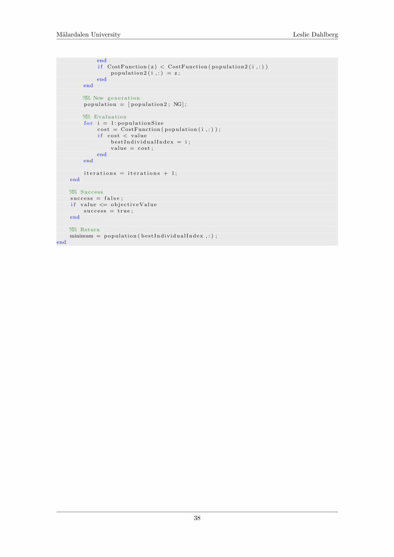
Malardalen University Leslie Dahlberg
endi f CostFunction ( z ) < CostFunction ( populat ion2 ( i , : ) )
populat ion2 ( i , : ) = z ;end
end
%% New genera t i onpopulat ion = [ populat ion2 ; NG] ;
%% Evaluat ionf o r i = 1 : popu la t i onS i z e
co s t = CostFunction ( populat ion ( i , : ) ) ;i f c o s t < value
be s t Ind iv idua l Index = i ;va lue = cos t ;
endend
i t e r a t i o n s = i t e r a t i o n s + 1 ;end
%% Successs u c c e s s = f a l s e ;i f va lue <= objec t i veVa lue
s u c c e s s = true ;end
%% Returnminimum = populat ion ( be s t Ind iv idua l Index , : ) ;
end
38