Evolving Trading Strategies Using Directional Changes

Michael Kampouridisa,∗, Fernando Oteroa

aSchool of Computing, University of Kent, UK

Abstract

The majority of forecasting methods use a physical time scale for studying price fluctuations of financial markets,making the flow of physical time discontinuous. Therefore, using a physical time scale may expose companies torisks, due to ignorance of some significant activities. In this paper, an alternative and original approach is exploredto capture important activities in the market. The main idea is to use an event-based time scale based on a new wayof summarising data, called Directional Changes. Combined with a genetic algorithm, the proposed approach aimsto find a trading strategy that maximises profitability in foreign exchange markets. In order to evaluate its efficiencyand robustness, we run rigorous experiments on 255 datasets from six different currency pairs, consisting of intra-daydata from the foreign exchange spot market. The results from these experiments indicate that our proposed approachis able to generate new and profitable trading strategies, significantly outperforming other traditional types of tradingstrategies, such as technical analysis and buy and hold.

Keywords: directional changes, financial forecasting, algorithmic trading, genetic algorithm

1. Introduction

The global financial system, recently rocked by the financial crisis, is open 24 hours a day, 7 days a week andcan be defined as a complex network of interacting agents (e.g., corporations, retail traders). With an average dailyturnover of 3–4 trillion USD (International Monetary Fund, 2009) and price changes nearly every second, its activityvaries at different times of a day and reacts on the announcement of political or economic news.

The majority of traditional methods to observe such price fluctuations in financial time series are based on phys-ical time change. For example, what researchers and practitioners tend to do is to use snapshots of the market, takenat fixed intervals; they first decide how often to sample the data, and then they take snapshots at the chosen fre-quency. Therefore, these snapshots create an interval-based summary—e.g. daily closing prices or minute-by-minutesummaries. However, important price movements (and thus potential profit) might be lost due to the creation of theseartificial price summaries. For example, if we are using daily closing price summaries we would not be able to observethe 6 May 2010 Flash Crash, which was a United States trillion-dollar stock market crash that lasted for approximately36 minutes.1

Directional Changes (DC) is based on the idea that an event-based system can capture significant points in pricemovements that the traditional physical time methods cannot. Hence, instead of looking the market from an interval-based perspective, DC record the key events in the market (e.g., changes in the stock price by a pre-specified percent-age) and summarise the data based on these events, moving away from a physical-time view to an event-based-timeview. Under this new paradigm, a threshold θ is defined, usually expressed by a percentage of the price. The marketis then fragmented and summarised into upward and downward trends. Different thresholds produce different pricesummaries. Thus, the directional changes paradigm focuses on the size of price change, while time is the varyingfactor; whereas in the physical-time paradigm, time was fixed (e.g. daily closing prices). This new concept provides

∗Corresponding author. Tel: +44 1634 8888 37Email addresses: M.Kampouridis@kent.ac.uk (Michael Kampouridis), F.E.B.Otero@kent.ac.uk (Fernando Otero)

1http://blogs.wsj.com/marketbeat/2010/05/11/nasdaq-heres-our-timeline-of-the-flash-crash/

Last access: 12 September 2016.

Preprint submitted to Expert Systems with Applications December 23, 2016

traders with new perspectives to price movements, and allows them to focus on those key points than an importantevent took place, blurring out other price details which could be considered irrelevant, or even noise.

The first works to use the concept of directional changes were proposed in Olsen et al. (1997) and Glattfelderet al. (2011). In these works, new empirical scaling laws in foreign exchange data series were discovered. Thesescaling laws aimed to establish mathematical relationships among price moves, duration and frequency. Then, di-rectional changes and the scaling laws from the above works were used to develop new trading models in Dupuis &Olsen (2012). However, those models were not used for any financial forecasting purposes and were only used toderive statistics from potential trading. Furthermore, Aloud et al. (2012) demonstrated the effectiveness of directionalchanges in capturing periodic market activities. In addition, Gypteau et al. (2015) presented an approach to forecastingthe daily closing price of financial markets by combing directional changes and genetic programming. Lastly, Tsanget al. (2016) introduced new trading indicators for profiling markets under directional changes. As we can observe, themajority of the above works have focused on theoretical aspects of directional changes—e.g. establishing mathemat-ical relationships and developing new indicators. Only Dupuis & Olsen (2012) and Gypteau et al. (2015) attemptedto generate trading strategies based on the DC concept. However, Dupuis & Olsen (2012) did not take advantage ofthe combined knowledge that can exist by using multiple DC thresholds to generate different event-based series; inaddition, Gypteau et al. (2015) only tested their approach on 4 datasets on daily closing prices.

In this paper our aim is to offer a more complete analysis on the directional changes paradigm from a financial fore-casting perspective. We run extensive tests on intraday data from six currency pairs from the foreign exchange (FX)market: yearly tick data from GBP/JPY, and yearly 10-minute interval data from EUR/GBP, EUR/USD, EUR/JPY,GBP/CHF, and GBP/USD. In total, we run tests on 255 different datasets. In terms of DC, we present two noveltypes of trading strategies: a single-threshold DC strategy, and a multi-threshold DC strategy. The former uses a sin-gle threshold to generate event-based series. The multi-threshold strategy combines different thresholds, where eachthreshold generates a different event-based series; then information from each series is aggregated to form a moreinformed trading strategy. In addition, we use a genetic algorithm (GA), which is a bio-inspired algorithm mimickingan evolutionary process, to optimise the parameters of the multi-threshold strategy. Such evolutionary algorithmshave extensively been used in financial forecasting problems and have shown to be extremely effective (Kwon &Moon, 2007; Mani, 1996; Evans et al., 2013; Kampouridis & Otero, 2015). The GA-generated trading strategies arethen compared against the single-threshold and the multi-threshold DC strategies. We test the GA-generated tradingstrategies with other financial benchmarks, such as buy and hold and technical analysis strategies. Overall, our goalsin this work can be summarised as follows: (i) demonstrate that the paradigm of DC returns profitable strategies,(ii) provide evidence that the strategies optimised by the GA are more profitable than using standard DC strategies,and (iii) demonstrate that our GA generated strategies outperform classical physical-time based strategies, namelytechnical analysis and buy and hold.

Lastly, it should be acknowledged that directional changes has similarities to the concept of the zigzag indicator(Azzini et al., 2010), which also focuses on an event-based approach, and to the concept of perceptually importantpoint (PIP) identification (Chen & Chen, 2016), which preserves the salient points in a time series to reduce the numberof data points. However, as we’ve mentioned above, the recent research on the DC field has led to the developmenton many new concepts, such as the scaling laws and new trading indicators that only exist under DC price summaries.Thus, in order to take advantage of all these new developments, we are focusing on the DC paradigm.

The rest of this paper is organised as follows: Section 2 presents background information in the fields of financialforecasting, directional changes, and genetic algorithms. Then, Section 3 presents the proposed DC-derived tradingstrategies, and Section 4 discusses how we used the genetic algorithm to optimise the parameters of these strategies. Inaddition, Section 5 presents the experimental setup, and Section 6 presents and discusses the results. Finally, Section7 concludes the paper and discusses directions for future work.

2. Background

Financial forecasting is a vital area in computational finance (Tsang & Martinez-Jaramillo, 2004). The end goalof financial forecasting is deriving a trading strategy, which makes a recommendation whether to buy, hold or sell.There are numerous works that attempt to return profitable trading strategies—several examples can be found in Chen(2002); Binner et al. (2004); Hu et al. (2015); Jaisinghani (2016).

2

There are several different strategies for the purposes of trading in a financial market. A very common investmentstrategy, albeit a passive one, is buy and hold, and commonly acts as benchmark for trading algorithms. The principleof this strategy is based on the view that in the long run financial markets give a good rate of return to investors. Thus,in this strategy an investor buys an asset and holds it for a long time, without being concerned about short-term pricemovements. Then at the end of a given period, s/he sells the stock and potentially makes profit based on the pricedifference.

In contrary to buy and hold, there is also the belief that it is profitable to take advantage of short-term pricemovements, as long as one can anticipate/predict them. Technical analysis is such a technique, and is discussed inSection 2.1. Then, we present background information on directional changes, a new way of summarising financialdata that can lead to new types of trading strategies. This takes place in Section 2.2. Finally, Section 2.3 gives anoverview of genetic algorithms, which is the technique used in this paper for optimising the use of directional changesparameters.

2.1. Technical analysis

Technical analysis is a methodology for financial forecasting. This method assumes that patterns exist in historicalprice data and that these patterns will repeat themselves. Consequently, it is worth identifying these patterns, so thatwe can exploit them in the future and make profit. Several works exist that are using technical analysis—recentexamples can be found in Cervelló-Royo et al. (2015); Chourmouziadis & Chatzoglou (2016).

As part of technical analysis, several indicators are used. These technical analysis indicators are formulas thatmeasure different aspects of a given financial dataset, such as trend, volatility and momentum. Below in Equations(1)-(6) we present 6 popular indicators that can be found in the literature (Martinez-Jaramillo, 2007; Allen & Kar-jalainen, 1999; Austin et al., 2004). Given a price time series [P(t), t ≥ 0], and a period of length L, these indicatorsare defined as follows:

Moving Average (MA)

MA(L,t) =P(t) − 1

L

L∑i=1

P(t − i)

1L

L∑i=1

P(t − i)(1)

MA allows traders to observe any changes in the trend of the prices of a stock. Typically, when a short-term MA (e.g.,12 days) goes above a long-term MA (e.g., 60 days), this indicates upward momentum. On the other hand, when ashort-term MA goes below a long-term one, this indicates downward momentum.

Trade Break Out (TBR)

TBR(L,t) =P(t) −max{P(t − 1), . . . ,P(t − L)}

max{P(t − 1), . . . ,P(t − L)}(2)

In order to understand this indicator better, we first need to explain two terms: support and resistance. Support is thepoint where the price stops going down any further, whereas resistance is the point where the price does not go upany further. Technical analysis suggests that downward price trends tend to reverse at support points, whereas upwardtrends tend to reverse at resistance points. However, when these points are breached (breakout), perhaps because ofsome new information regarding the market, it is likely that the price will continue in the same direction. Hence,traders tend to observe these breakouts and when a stock goes above its point of resistance, they buy; when on theother hand the stock price goes below its point of support, traders sell.

Filter (FLR)

FLR(L,t) =P(t) −min{P(t − 1), . . . ,P(t − L)}

min{P(t − 1), . . . ,P(t − L)}(3)

3

This indicator is used to indicate buy or sell actions, depending on whether the price movement goes in the oppositedirection by a predefined percentage. For instance, if the price reverses from a downward trend and rises by a specificpercentage from the low price that it was previously, then the trader would perform a ‘buy’ action.

Volatility (Vol)

Vol(L,t) =σ(P(t), . . . ,P(t − L + 1))

1L

L∑i=1

P(t − i)(4)

A period of an increasing volatility could indicate a reversal in the trend or strong downward trends. This wouldthus give an indication to a trader that s/he should be cautious. On the contrary, when there is a period of decreasingvolatility, this indicates upward trends and traders should buy.

Momentum (Mom)

Mom(L,t) = P(t) − P(t − L) (5)

When Mom is positive, this indicates an upward trend. If Mom starts decreasing, this could be an indication that thereis going to be a reverse in the previously upwards trend, and hence the traders should be cautious. Finally, when Momis negative, this indicates a downwards trend.

Momentum Moving Average (MomMA)

MomMA(L,t) =1L

L

∑i=1

Mom(L, t − i) (6)

Finally, from Mom we can also calculate its MA, as shown in the above equation, which allows us to obtain summariesof the Momentum movements.

While the above indicators can offer valuable information, normally a trader would use many of these indicatorstogether, thus combine their recommendations. It is very common in the literature to use machine learning algorithmsto combine technical information indicators (Chiang et al., 2016; Kim & Enke, 2016). In this work, we use EDDIE(Kampouridis & Tsang, 2012, 2010) as a baseline algorithm. EDDIE is a genetic programming (GP) (Koza, 1992)financial forecasting algorithm, which combines the different technical analysis indicators together, in order to formpredictions. The advantage of combining technical analysis indicators is that their combined knowledge can lead tobetter predictions. We should also mention that EDDIE has been used over the years for different types of financialproblems, such as stock price movement prediction (Kampouridis & Otero, 2015), arbitrage opportunities detection(Tsang et al., 2005), and market crash detection (Garcia-Almanza et al., 2013). EDDIE has thus extensively andeffectively utilised technical analysis for its predictions, and for this reason we have chosen to use it as a benchmarkof an algorithm using technical analysis.

As EDDIE is a GP algorithm, its trading strategies are represented as trees. A sample tree of EDDIE is presentedin Figure 1. As we can see, if the 20 days MA is less than or equal to 6.4, then the user is advised to buy; otherwise,the user is advised to consult another tree, which is located in the third branch (“else-branch”) of the tree. This treechecks if the 50 days MomMA is greater than 5.57; if it is, it advises to not-buy, otherwise to buy. Of course this issimply a sample tree; so additional/different technical analysis indicators could be used in other trees.

In summary, what we have presented so far—namely buy and hold, technical analysis and EDDIE—all use in-formation derived from data that is based on physical-time. As we have explained, in this paper we propose usingevent-based price summaries for creating the trading strategies, based on the concept of directional changes.

4

If

<=

VarConstructor

MA 20

6.64

Buy(1) If

>

VarConstructor

MomMA 50

5.57

Not-Buy(0) Buy(1)

Figure 1: Sample tree generated by EDDIE representing a trading strategy using technical indicators.

2.2. Directional changesThe directional change (DC) approach is an alternative approach for summarising market price movements. A DC

event is identified by a change in the price of a given financial instrument. This change is defined by a threshold value,which was in advance decided by the trader. Such an event can be either an upturn or a downturn event. After theconfirmation of a DC event, an overshoot (OS) event follows. This OS event finishes once an opposite DC event takesplace. The combination of a downturn event and a downward overshoot event represents a downward trend and, thecombination of an upturn event and an upturn overshoot event represents an upturn trend. In other words, a downwardtrend is a period between a downturn event and the next upturn event and an upturn trend is a period between an upturnevent and the next downturn event.

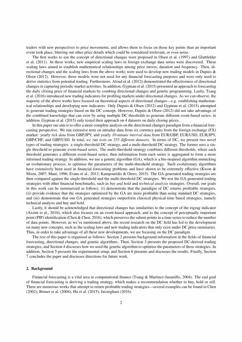
Figure 2 presents an example of how a physical-time price curve is transformed to the so-called intrinsic time(Glattfelder et al., 2011) and dissected into DC and OS events. As we can observe, two different thresholds are used,and each threshold generates a different event series. Thus, each threshold produces a unique series of events. Theidea behind the different thresholds is that each trader might consider different thresholds (price percentage changes)as significant. A smaller threshold creates a higher number of directional changes, while a higher thresholds producesfewer directional changes.

Looking at the events generated by a threshold of θ = 0.01% (events connected via solid and dashed lines), wecan observe that any price change less than this threshold is not considered a trend. On the other hand, when the pricechanges above that threshold, then the market is divided accordingly, to uptrends and downtrends. DC events are insolid lines, and OS events are in dashed lines. So an downturn DC event starts at Point A and lasts until Point B,when the downturn OS events starts. The downturn OS lasts until Point C, when there is a reverse in the trend, and anuptrend starts, which lasts until Point D. From Point D to E we are in an upturn OS event, and so on.

As we mentioned, different thresholds generate different event series. Looking at theta = 0.018% (events con-nected via dotted and dot-dashed lines), we can observe that the events generated are different: a downward trendstarts from A and lasts until B′, and the downward OS is from Point B′ until C. Then, from Point C until Point E thereis an upward DC trend, and from E to E′ there’s an upward OS trend. Algorithm 1 presents the high-level pseudocodefor generating directional changes events.

It is important to note here that the confirmation of a change of a trend can only be confirmed retrospectively, i.e.only after the price has changed by the pre-specified DC threshold value θ. For example, under θ = 0.01% we can onlyconfirm that we are in a upward trend from Point D onwards. Point D is thus called a confirmation point. Before PointD, the directional change had not been confirmed (i.e. the market price had not changed by the pre-specified thresholdvalue), thus a trader summarising the data by the DC paradigm would continue believing we are in a downward trend,which started from Point A. Similarly, a trader using θ = 0.01% would continue considering being in a upward trendfrom Point D until the price has reversed by θ = 0.01%, which only takes place at the next confirmation point, i.e.,Point F. So what becomes important here is to be able to anticipate the change of the trend as early as possible, i.e.before Points C and E have been reached. In addition, since different thresholds generate different event series, wehypothesise that the combined information from these series would lead to profitable trading strategies.

5

Figure 2: Directional changes for tick data for the GBP/JPY currency pair. The solid and dashed lines denote a set of events defined by a thresholdθ = 0.01%, while the dotted and dot-dashed lines refer to events defined by a threshold θ = 0.018%. The solid and the dotted lines indicate theDC events, and the dashed and dot-dashed indicate the OS events. Under θ = 0.01%, the data is summarised as follows: Point A↦ B (Downwarddirectional change), Point B↦ C (Downward overshoot event), Point C↦ D (Upward directional change), Point D↦ E (Upward overshoot event),Point E↦ F (Downward directional change). Under θ = 0.018%, the data is summarised as follows: Point A↦ B’ (Downward directional change),Point B’↦ C (Downward overshoot event), Point C↦ E (Upward directional change), Point E↦ E’ (Upward overshoot event).

The advantage of this new way of summarising data is that it provides traders with new perspectives to pricemovements, and allows them to focus on those key points that an important event took place, blurring out other pricedetails which could be considered irrelevant or even noise. Furthermore, DC have enabled researchers to discover newregularities in markets, which cannot be captured by the interval-based summaries (Glattfelder et al., 2011). Therefore,these new regularities give rise to new opportunities for traders, and also open a whole new area for research.

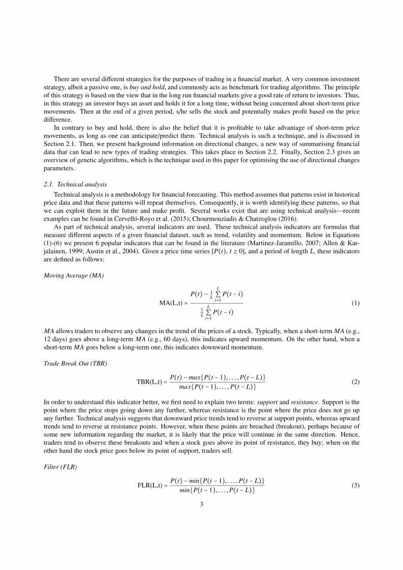
One of the most interesting regularities that was discovered in Glattfelder et al. (2011) was the observation that aDC of threshold θ is on average followed by an OS event of the same threshold θ. At the same time, it was observedthat if on average a DC takes t amount of physical time to complete, the OS event will take an amount of 2t. Thisobservation is summarised in Figure 3, and was only made under DC-based price summaries, and not under phsycical-time summaries. Furthermore, this astonishing observation was made on all of the 13 different currency exchangerates that the authors of Glattfelder et al. (2011) experimented with. This thus leads us to further hypothesise that suchstatistical properties could lead to profitable strategies, if appropriately exploited, mainly because such properties arenot well-known to traders yet. Therefore, the DC area is a rich research area that could potentially lead to significantdiscoveries.

In this work, we will present new trading strategies based on the concept of directional changes. As part of theimplementation of this trading strategy we will be using the scaling law presented above; we have also introducedseveral parameters into the system, which we present in detail in Section 3.

Lastly, since a user/trader has to decide on which thresholds to use for generating DC events, a problem that arisesis what are appropriate thresholds and how much weight we should give to the information provided by each threshold.We are thus faced with an optimisation problem, where one has to look into the space of different thresholds and focuson the most promising ones. One of the popular optimisation techniques is Genetic Algorithms, discussed next.

2.3. Genetic algorithmsGenetic Algorithms (GAs) are bio-inspired algorithms that mimic an evolutionary process to find good solutions

to optimisation problems (Godlberg, 1989; Mitchell, 1996; Michalewicz, 2002). GAs have several elements thatallow them to perform a robust global search: (a) they work with a population of candidate solutions (individuals),rather than a single candidate solution; (b) individuals of the population are evaluated according to a fitness function,

6

Figure 3: An example of a scaling law presented in Glattfelder et al. (2011), which shows that (1) a DC event (solid line) of threshold θ is followedby an OS event (dotted line) of also threshold θ, and (2) the OS event lasts about the double amount of time that it took for the DC event to takeplace.

Algorithm 1 Pseudocode for generating directional changes events (source: Aloud et al. (2012)).

Require: Initialise variables (event is Upturn event, ph = pl = p(t0),∆xdc(Fixed) ≥ 0, tdc0 = tdc

1 = tos0 = tos

1 = t0)1: if event is Upturn Event then2: if p(t) ≤ ph × (1 − ∆xdc) then3: event ← DownturnEvent4: pl ← p(t)5: tdc

1 ← t // End time for a Downturn Event6: tos

0 ← t + 1 // Start time for a Downward Overshoot Event7: else8: if ph < p(t) then9: ph ← p(t)

10: tdc0 ← t // Start time for Downturn Event

11: tos1 ← t − 1 // End time for an Upward Overshoot Event

12: end if13: end if14: else15: if p(t) ≤ pl × (1 + ∆xdc) then16: event ← U pturnEvent17: ph ← p(t)18: tdc

1 ← t // End time for a Upturn Event19: tos

0 ← t + 1 // Start time for an Upward Overshoot Event20: else21: if pl > p(t) then22: pl ← p(t)23: tdc

0 ← t // Start time for Upnturn Event24: tos

1 ← t − 1 // End time for an Downward Overshoot Event25: end if26: end if27: end if

7

which measures the quality of the candidate solution represented by an individual—the higher their quality, the morelikely that their genetic material will be carried forward to the next population; (c) the solution space is exploredusing genetic operators, which generate new offspring individuals from individuals of the current population using astochastic selection procedure based on fitness.

Algorithm 2 presents a high-level pseudocode of a GA. The algorithm starts by creating a population of p candidatesolutions, where p is referred to as population size. These are evaluated by a fitness function in order to determine theirperformance in solving the problem at hand. On each iteration (while loop), a new population is then generated byprobabilistically selecting the fitter individuals from the current population. Some of the selected individuals undergocrossover and mutation, which introduce modification to explore the search space; other are carried forward withoutmodifications. The new population replaces the old and the new individuals are evaluated. This process is repeateduntil a maximum number of generations is reached or the (near-)optimal solution is found, acting as a terminationcondition. Through this evolutionary process, GAs perform a robust global search in the space of candidate solutions,less likely to get trapped into local minima.

Representation. Individuals in GAs are usually represented as a string of symbols, either binary or numeric values—the representation is dependant on the problem at hand. Figure 4 shows an illustration of a real-valued representation.Each position in the string is referred to as a gene and it represents a variable to be optimised. At the start of a GA,the population is initialised with random individuals: each gene is initialised with a random value in the domain ofthe variable.

Genetic Operators. Genetic operators manipulate the genetic material of individuals (strings of symbols) to generatenew offspring individuals, mimicking a mechanism of inheritance. For example, crossover create two new offspringsolutions from two parent individuals by swapping portions of genetic material (or genes) from each parent. Toillustrate, consider the uniform crossover operator in Figure 4. This operator combines genes sampled uniformlyfrom two parents. In addition to crossover, GAs usually employ a mutation operator, which produces a new offspringindividual from a single parent. In uniform mutation, small changes are introduced to a parent individual by choosingand modifying each gene at random. Both uniform crossover and uniform mutation are controlled by two probabilitiesrates: the first one is used to decided whether the selected individual will undergo crossover/mutation (pc and pm inAlgorithm 2, respectively) or not; the second rate is used to decide if a gene is swapped/mutated or not. Figure 4shows an illustration of both uniform crossover and uniform mutation operators.

Elitism and Selection. Elitism is the process of allowing the best individuals (in terms of fitness) of the currentpopulation to be carried over to the next without modification. This guarantees that the solution fitness will notdecrease from one generation to the next. The remaining individuals are subject to a probabilistic selection forinclusion in the next generation population. One of the most popular selection strategies is the tournament selection.In tournament selection, k individuals are selected at random, where k denotes the tournament size. The more fitindividual of the selected subset is then selected for inclusion in the next population.

2.4. Summary

In this section we started by discussing two popular trading techniques, namely buy and hold and technical anal-ysis. Both of these two methods will form our financial benchmarks during our experimental phase. In addition, wepresented in detail the concept of directional changes, which our trading strategies are going to be based on. Lastly,we discussed what genetic algorithms are, as they are going to be our optimisation engine. In the next section, wepresent two new types of trading strategies, which are derived by directional changes.

3. DC-derived trading strategies

In this section, we will present how we can use the DC paradigm to derive two different types of trading strategies.The first one is going to be based on a single DC threshold, and is going to be presented in Section 3.1. The secondstrategy is going to be based on multiple DC thresholds and is going to be presented in Section 3.2.

8

Algorithm 2 High-level pseudocode of a genetic algorithm.GA(p, Fitness, pc, pm)

p: population sizeFitness: determines the quality of solutionspc: crossover ratepm: mutation rate

1: Initialise population: P← Generate p individuals (candidate solutions) at random2: Evaluate: for each i in P, calculate Fitness(i)3: while termination condition not satisfied do4: Pg ← Create new population for generation g

(a) Elitism: copy the r best individuals from P to Pg

(b) Select: probabilistically select (p − r) individuals of P to add to Pg and• Perform crossover between a pair of selected individuals according to pc• Perform mutation on a selected individual according to pm

5: Update: P← Pg

6: Evaluate: for each i in P, calculate Fitness(i)7: end while8: Return the individual with the highest fitness from P

0.7 0.3 0.5 0.4 0.2 0.1 0.9 0.6

0.3 0.1 0.8 0.9 0.4 0.2 0.7 0.6 0.7 0.1 0.8 0.4 0.4 0.1 0.9 0.6

0.5 0.1 0.4 0.2 0.1 0.7 0.2 0.8 0.5 0.1 0.7 0.2 0.6 0.7 0.2 0.1

0.3 0.3 0.5 0.9 0.2 0.2 0.7 0.6

Uniform crossover:

Uniform mutation:

Parent individuals Offspring

Figure 4: Illustration of uniform crossover and uniform mutation operators. Individuals are represented as a string of real values. The dark positions(genes) in parent individuals are the ones that will be swapped/mutated to generate offspring individuals.

9

3.1. Single-threshold DC trading strategy

As we have already discussed in Section 2.2, a physical-time price curve can be transformed to intrinsic time,where it’s dissected into DC and OS events. When a DC event is confirmed (either upturn or downturn), the OSperiod starts. It is worth re-iterating that we can only know the market has changed direction in hindsight; we onlydetect a DC event only after the DC confirmation point has been observed. After the DC confirmation has taken place,we are during an OS period, which lasts until there is a reverse in the direction, which is again only confirmed oncewe have reached the next confirmation point. Therefore, if one can act during the OS period and before the reverse ofthe trend, then this can lead to a profitable trading strategy. The idea is that if we are in an downtrend, we buy at thelast point (ideally) of the OS event, which is the lowest observed value. When the trend then reverses and we are inan uptrend, we can then sell at a much higher price and make profit. The same principle applies for uptrend: sell asclose as possible to the end of the OS event. To sum up, when there is a downtrend, we buy; when there is an uptrend,we sell.

In order to make the above clearer, let us refer back to Figure 2. As we can observe, after the confirmation of thedownward trend in Point B, a period of OS starts, which lasts until Point D, which is the next DC confirmation point,confirming that we are now in a upward trend. It is thus important to take a buy action during the OS event and ideallybefore the reverse of the trend, which as we can see takes place at Point C. The closer to the end of the OS event wecan trade (i.e., the closer to Point C), the higher the profit margin a trader can make.

Thus, it is crucial to be able to anticipate the reverse in the trend and be able to act before that. In order to tacklethis, we use the scaling laws we discussed earlier in Section 2.2. As explained, these laws states that when on averagea DC event takes t amount of physical time to complete, the OS event takes an amount of 2t. Because this is anapproximation and it can rely on the underlying dataset, we wanted to have our own calculations for the datasets weare dealing with. Thus, what we did was to calculate the average time of each OS event for every period we woulduse as a training set. We hence created two variables, expressed as the average ratio of the OS event length over theDC event length. These two variables are ru and rd, where ru is the average ratio of the upwards OS event, and rd

is the average ratio of the downwards OS event. Our calculations showed that these two variables had indeed valuesaround 2 (ranging between 1.8–2.0), which confirms the scaling law findings. More importantly, this allowed us tohave tailored values for ru and rd, for each training set we use.

After obtaining these ratios, we were able to anticipate the end of a trend (approximately) and as a result maketrading decisions once an OS event had reached the average ratio of ru or rd. Of course, in reality things are not thatsimple. The ru and rd ratios are just average approximations, so many times the OS event might last longer or shorterthan anticipated. In an attempt to address this issue, we have created two user-specified parameters, namely b1 andb2, which define a range of time within the OS period, where trading is allowed. For instance, if a trader expects theOS event to last for 2 hours, then we can define an action range of [b1,b2] = [0.90,1.0], which effectively means weare going to trade at the last 10% of the 2 hours duration, i.e. in the last 12 minutes. By introducing b1 and b2, we areessentially attempting to anticipate the approximation errors that might have been created during the calculation of ru

and rd. Equation 7 presents the formulas for these starting and ending for upward and downward OS periods:

tU0 = (tdc

1 − tdc0 ) × ru × b1

tU1 = (tdc

1 − tdc0 ) × ru × b2

tD0 = (tdc

1 − tdc0 ) × rd × b1

tD1 = (tdc

1 − tdc0 ) × rd × b2

, (7)

where tU0 , t

U1 are the start and end times for upwards overshoot period, respectively, and tD

0 , tD1 are the start and end

times for downwards overshoot period, respectively. In addition, tdc0 and tdc

1 are the start and the end times of thecurrent DC event, after the confirmation of the event has taken place at time tdc

1 . Their difference tdc1 − tdc

0 returnsthe length of the current DC event. Also, ru and rd are the average ratios of the upwards and downwards OS periodlengths, respectively, over the current DC period. Lastly, b1 and b2 are the two parameters defining the action rangewithin the OS periods, as explained above.

Although b1 and b2 define a window for trading, a problem that exists with high-frequency data—particularly tickdata—is that there can still be hundreds of points to trade, even if that trading window is very narrow. This could

10

Table 1: DC strategy parameters.

Parameter Description

ru Average ratio of upwards OS event over the upwards DC event lengthrd Average ratio of downwards OS event over the downwards DC event lengthQtrade Quantity to tradeN↓ Number of thresholds recommending to buyN↑ Number of thresholds recommending to sellNθ Total number of thresholds used in the experimentsQ Quantity for tradingb1 Start of trading period during an OS eventb2 End of trading period during an OS eventb3 Range of prices close to the trading price Ptrade that a trade can be perfomed

be problematic, because trading at multiple price levels will not return the highest profit. What is more effective isto sell (buy) at a price as expensive (cheap) as possible. To achieve this, we introduced another variable b3, whichprevents traders from doing expensive trades. To ensure this, we only allow the system to sell at the most expensive(peak) price Ppeak and buy at the cheapest recorded price (trough) Ptrough, or in prices in close range. This range isdetermined by the value of b3. Therefore a trader would sell when the price is equal to Ppeak × b3, or buy when theprice is equal to Ptrough × (1 − b3). Essentially, b3 is a value within the range of [0,1] and defines the range of pricesclose to Ppeak andPtough that the system will perform an action.

Furthermore, there is a user-specified parameter Q, which controls the trading quantity. Lastly, it should bementioned that our system allows short selling. However, in order to avoid excess short selling, which can lead tosignificant losses, we have introduced a stop loss mechanism that is called short selling allowance. This allowance isa percentage of our budget and allows short selling activities up to this pre-specified percentage. This percentage isdecided during parameter tuning.

3.2. Multi-threshold DC trading strategy

This strategy builds on the previous one, as it still uses Equation 7 and the b3 variable. But instead of only usinga single threshold, it combines information by multiple thresholds. As we discussed in Section 2.2, a DC event isidentified by a change in the price by a given threshold value. The use of different DC thresholds provides a differentview of the data: smaller thresholds allow the detection of more events and, as a result, actions can be taken promptly;larger thresholds detect fewer events, but provide the opportunity of taking actions when bigger price variations areobserved. This proposed trading strategy combines the use of different threshold values in an attempt to take advantageof the different characteristics of smaller and larger thresholds.

From the single-threshold strategy we know that under a specific threshold we should buy towards the end of adowntrend and sell towards the end of an uptrend (i.e. towards the end of the respective OS events). Since now we aredealing with multiple thresholds, each threshold summarises the data in a unique way. For example, at one point intime the trading strategy under one threshold could be recommending a buy action, while under a different thresholdrecommend a sell action. As we have already argued, the advantage of having the multiple thresholds is that we havemultiple recommended actions per data point. In order to decide which action to follow, a majority vote takes place.

In order to allow for a majority vote, we associate each DC treshold to an equal weight of 1 (vote). Therefore,W1 = W2 = W3 = ... = WNθ

= 1, where Nθ is the total number of thresholds used. As a result, at any point intime the trading strategy is able to make a buy/sell/hold recommendation based on the combined recommendationsof all thresholds. As we already know, each threshold produces DC events; thus each threshold is able to make thisbuy/sell/hold recommendation. Since we have Nθ thresholds, this means that at any point in time we receive Nθ

11

recommendations. In order to decide which recommendation to follow, we sum the weights of the thresholds: if thesum of the weights for all thresholds recommending a buy (sell) action is greater than the sum of the weights forall thresholds recommending a sell (buy) action, then the strategy’s action will be to buy (sell). The hold action is aspecial case of both buy and sell and it happens when we are outside the price range recommended by b3, or whenthere is not enough quantity to act, see Algorithm 4 lines 8, 11, and 26.

In addition, the multi-threshold trading strategy is able to make recommendations on the trading quantity Qtrade.The decision for this quantity is a dynamic decision, taken by the number of DC thresholds that are advising to sell(buy) at a certain point in time: if many thresholds are advising to sell (buy), then the algorithm sells (buys) a higherquantity of the given currency pair. Equations 8a and 8b present the relevant formulas, for buy and sell, respectively:

Qtrade = (1 +N↓Nθ

) × Q (8a)

Qtrade = (1 +N↑Nθ

) × Q (8b)

where Qtrade is the quantity to trade, N↓ and N↑ are the number of thresholds recommending to buy and sell, re-spectively, Nθ is the total number of thresholds used in our experiments, and Q is the user-specified quantity alreadypresented in Section 3.1. As we can see, by taking into account the recommendations given by the DC thresholds, weare giving more or less weight to the Q quantity, resulting to a new quantity Qtrade.

This concludes the presentation of the two proposed DC strategies and their respective parameters. For the con-venience of the reader, we have summarised and listed these parameters in Table 1. We have also summarised thetrading strategy processes into pseudocodes: Algorithm 3 presents an overview of how the return of a trading strategyis calculated. In addition, Algorithm 4 presents how the buy and sell actions take place. While these algorithms arefor the multi-threshold strategy, they can also be applied to the single-threshold strategy, where there is only a singleweight (for the single threshold) of W1 = 1 and Qtrade = Q.

4. Optimising multi-threshold strategies via a Genetic Algorithm

In the previous section, we presented two novel trading strategies based on the DC paradigm: a single-thresholdstrategy and a multi-threshold strategy that builds on top of the single-threshold. While the multi-threshold strategyhas the advantage of combining recommendations from different thresholds, a problem that exists is that we do notknow how much weight we should give to each threshold. Simply assigning an equal weight of 1 to all of thethresholds might be a naive approach. Some thresholds might be more useful than others, hence we should give themmore weight. Thus, we use a genetic algorithm (GA) to evolve real values for the weight of each DC threshold. Inaddition, we also evolve some other DC parameters that are crucial to the success of the trading strategy. All these arediscussed next, in Section 4.1, where the GA representation is presented. Then, Section 4.2 presents the GA operatorsand Section 4.3 presents the fitness function.

4.1. Representation

Each chromosome consists of 4 + Nθ genes, where Nθ is the number of different threshold values of the multi-threshold strategy. The number 4 denotes that in addition to the thresholds, there are also 4 additional parametersto be optimised: Q (first gene), b1 (second gene), b2 (third gene), and b3 (fourth gene). Q,b1,b2 and b3 refer to theDC-related parameters presented in Section 3.1. Each remaining gene in the chromosome (positions 5 to [4+Nθ])represents a weight associated to a given threshold. Thus, after first deciding the DC threshold values (throughparameter tuning) and generating the DC events per threshold, each GA gene is assigned the same initial weight.Therefore, W1 = W2 = W3 = ... = WNθ

= 1Nθ

. The GA then evolves the weight for each threshold (in addition to the 4parameter values in positions 1-4).

As a result, at any point in time a GA individual is able to make a buy/sell/hold recommendation based on thecombined recommendations of all thresholds by using the majority vote mechanism we presented in Section 3.2. Anexample of an 8-gene GA chromosome is presented in Figure 5.

12

Algorithm 3 Pseudocode for calculating the return of a trading strategy.Require: Initialise variables (cash = budget,Qtrade = 0, current = 0)Require: b1,b2, b3, Q and weight values W1 = W2 = ... = WNθ

= 1 for each threshold1: for i = 0; i < dataset_length; i + + do2: Initialise variables weights for buy and sell: WB = WS = 0, number of upturn and downturns: N↑ = N↓ = 03: current ← current + 14: if PC > Ppeak then //PC is the current price and Ppeak is the highest so-far price.5: Ppeak ← PC

6: else if PC < Ptrough then7: Ptrough ← PC

8: end if9: for j = 0; j < Nθ; j + + do

10: Calculate tU0 , t

U1 , t

D0 , t

D1 as explained in Equation 7

11: if event is Downturn Event then12: WB ←WB +W j

13: if current within range of [tD0 , t

D1 ] then

14: N↓ ← N↓ + 115: else16: N↓ ← N↓ − 117: end if18: else19: WS ←WS +W j

20: if current within range of [tU0 , t

U1 ] then

21: N↑ ← N↑ + 122: else23: N↑ ← N↑ − 124: end if25: end if26: end for27: if WS > WB then28: Perform the sell action for a given quantity [see Algorithm 4]29: else if WS < WB then30: Perform the buy action for a given quantity [see Algorithm 4]31: end if32: end for33: Wealth← cash + Qtrade × PC

34: Return← 100 × wealthbudget

Figure 5: An example of a 8-gene GA chromosome. The first four genes are : Q, b1, b2 and b3, respectively. The remaining four genes are theweights for the DC thresholds: W1,W2,W3, and W4.

13

Algorithm 4 Pseudocode for performing the buy and sell actions.1: if WS > WB then2: if N↑ > 0 and PC ≥ b3 × Ppeak then3: Qtrade ← (1 + N↑

Nθ) × Q

4: if Qtrade > 0 or (Qtrade ≤ 0 and ∣Qtrade∣ × PC ≤ shortS ellingAllowance × budget) then5: Cash← Cash + Qtrade × PC

6: PFL ← PFL − Qtrade // PFL stands for Portfolio, i.e. the amount/quantity of the currency pair we arecurrently holding

7: else8: Hold9: end if

10: else11: Hold12: end if13: else if WS < WB then14: if N↓ > 0 and PC ≤ Ptrough + (Ptrough × (1 − b3)) then15: Qtrade ← (1 + N↓

Nθ) × Q

16: if cash > Qtrade × PC then17: Cash← Cash − Qtrade × PC

18: PFL← PFL + Qtrade

19: else20: // Buy only as much as you can afford21: Q′

trade is the new quantity to be traded, up to the amount we can afford22: Cash← Cash − Q′

trade × PC

23: PFL← PFL + Q′

24: end if25: else26: Hold27: end if28: end if

14

Based on this example, the GA recommends buying/selling a quantity of Q equal to 10, and only acting in theperiod [0.9,1.0] of the estimated duration of the OS event (i.e., in the last 10% of the length of the OS event). Inaddition, the fourth gene recommends to only consider prices that are within a 20% range (the value of b3 is 0.8,so 1.0 − 0.8 = 0.20 or 20%) of the highest (lowest) recorded price Ppeak (Ptrough). In addition, to decide the tradingaction, we would check the recommendation of each individual threshold. For this example, let us assume that thefirst threshold recommends buy, the second threshold recommends sell, the third threshold recommends buy, and thefourth threshold recommends hold. We would then sum up the weights of the thresholds, according to each action.Therefore, the weight for buying WB is equal to W1 +W3 = 0.2 + 0.2 = 0.4, and the weight for selling WS is equal toW2 = 0.5.2 Since WS > WB, the GA’s recommendation would be to sell.

4.2. Operators

The following three operators are being used during the evolutionary process: elitism, uniform crossover anduniform mutation—as detailed in Section 2.3.

In elitism, the best-performing individual (in terms of fitness) is copied to the next generation. In uniformcrossover, two parents are selected via a tournament selection. In this type of crossover, the genes between thetwo parents are swapped with a fixed probability of 0.5. In addition, we ensure that the value of the third gene isalways greater than the value of the second gene, i.e. b2 always has to be greater than b1. Lastly, for the uniformmutation operator a single parent is selected, again by tournament selection. With a probability of 0.5, each gene ofthe chromosome is mutated, and a different value is obtained. It should be clarified here that for the first gene (quantityQ), the mutated value can be any integer up to a pre-specified maximum quantity value; whereas for the remaininggenes (i.e., b1,b2,b3 and all weights W), the mutated values are real numbers between 0 and 1, where b2 > b1.

4.3. Fitness function

Several different metrics have been used in the literature as fitness function in algorithmic trading problems. Someexamples are: wealth, profit, return, Sharpe ratio, information ratio (Brabazon & O’Neill, 2006; Bradley et al., 2009).In this paper, we set our fitness equal to the total return minus the maximum drawdown, presented in Equation 9:

f f = Return − α ×MDD

MDD =Ptrough − Ppeak

Ppeak

, (9)

where Return is the return of the investment, MDD is the maximum drawdown, and α is a tuning parameter. Maximumdrawdown is defined as the maximum cumulative loss since commencing trading with the system. It is used to penalisevolatile trading strategies in terms of return. Its value is given as the percentage of Ptrough−Ppeak

Ppeak, where Ptrough the trough

value of the price, and Ppeak is the peak value of the price. Lastly, the tuning parameter α is used to define how muchrisk-averse the strategy is. The more risk-averse in terms of wishing to avoid a catastrophic loss, the higher the valueof α.

5. Experimental Setup

This section is divided into three parts: Section 5.1, where we present the data we use for our experiments, Section5.2, where we present the experimental setup, and lastly, Section 5.3, which presents the experimental parameters.

2As explained in the previous section, the hold action is an exceptional case that is considered as an alternative to buy and sell actions; seeAlgorithm 4, Lines 8, 11 and 26 for detail.

15

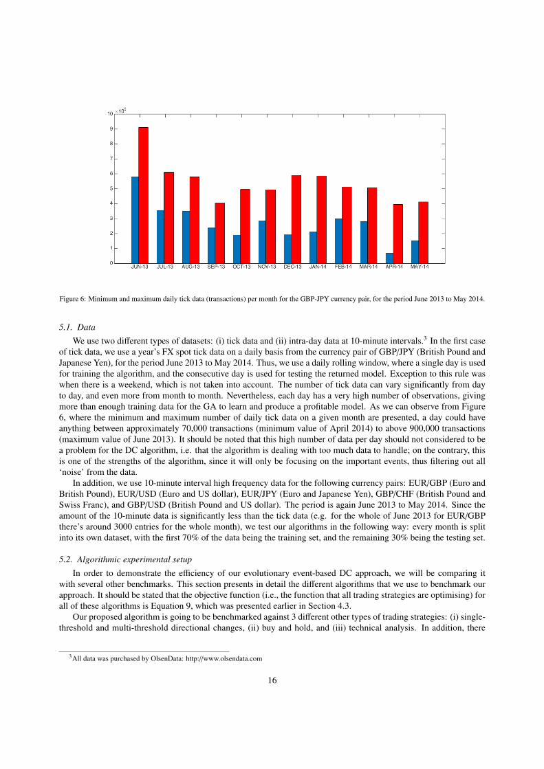
Figure 6: Minimum and maximum daily tick data (transactions) per month for the GBP-JPY currency pair, for the period June 2013 to May 2014.

5.1. Data

We use two different types of datasets: (i) tick data and (ii) intra-day data at 10-minute intervals.3 In the first caseof tick data, we use a year’s FX spot tick data on a daily basis from the currency pair of GBP/JPY (British Pound andJapanese Yen), for the period June 2013 to May 2014. Thus, we use a daily rolling window, where a single day is usedfor training the algorithm, and the consecutive day is used for testing the returned model. Exception to this rule waswhen there is a weekend, which is not taken into account. The number of tick data can vary significantly from dayto day, and even more from month to month. Nevertheless, each day has a very high number of observations, givingmore than enough training data for the GA to learn and produce a profitable model. As we can observe from Figure6, where the minimum and maximum number of daily tick data on a given month are presented, a day could haveanything between approximately 70,000 transactions (minimum value of April 2014) to above 900,000 transactions(maximum value of June 2013). It should be noted that this high number of data per day should not considered to bea problem for the DC algorithm, i.e. that the algorithm is dealing with too much data to handle; on the contrary, thisis one of the strengths of the algorithm, since it will only be focusing on the important events, thus filtering out all‘noise’ from the data.

In addition, we use 10-minute interval high frequency data for the following currency pairs: EUR/GBP (Euro andBritish Pound), EUR/USD (Euro and US dollar), EUR/JPY (Euro and Japanese Yen), GBP/CHF (British Pound andSwiss Franc), and GBP/USD (British Pound and US dollar). The period is again June 2013 to May 2014. Since theamount of the 10-minute data is significantly less than the tick data (e.g. for the whole of June 2013 for EUR/GBPthere’s around 3000 entries for the whole month), we test our algorithms in the following way: every month is splitinto its own dataset, with the first 70% of the data being the training set, and the remaining 30% being the testing set.

5.2. Algorithmic experimental setup

In order to demonstrate the efficiency of our evolutionary event-based DC approach, we will be comparing itwith several other benchmarks. This section presents in detail the different algorithms that we use to benchmark ourapproach. It should be stated that the objective function (i.e., the function that all trading strategies are optimising) forall of these algorithms is Equation 9, which was presented earlier in Section 4.3.

Our proposed algorithm is going to be benchmarked against 3 different other types of trading strategies: (i) single-threshold and multi-threshold directional changes, (ii) buy and hold, and (iii) technical analysis. In addition, there

3All data was purchased by OlsenData: http://www.olsendata.com

16

are 4 parameters for all DC configurations, which depending on the experimental setup, we optimise or not. These4 parameters are: Q, b1, b2, and b3. Please refer back to Section 3.1 for a detailed presentation of these parameters.Therefore, by taking the above parameters into account, we have the following different configurations, which willconstitute our different algorithmic experimental setups:

Standard directional changesThe purpose here is to present the results of the DC paradigm, under a single-threshold and a multi-thresholdframework. The values of thresholds were decided during the parameter tuning process.

1. Single-threshold, with no evolution (SDC)This is the trading strategy presented in Section 3.1. The 4 parameters [Q,b1,b2,b3] have not been optimisedand have fixed values: Q = 1,b1 = 0,b2 = 1,b3 = 1, which essentially allow trading of a single quantitythroughout the length of the OS event for any given price, no matter how expensive or cheap it is. Of course,this is not the optimal setup for these values and this is why in the next setup we evolve these parameters toobtain better values. However, we consider it important to report results from this setup of SDC to demonstratethat it is crucial to optimise the four parameters [Q,b1,b2,b3]. Lastly, in order to decide which (single) thresholdto use, we experiment with several different thresholds (one at a time) and report the performance of the bestthreshold.

2. Single-threshold, with evolution on the 4 parameters (S DCEVO)As above. The difference is that now we use a standard GA to evolve the values of the 4 numeric parame-ters [Q,b1,b2,b3]. The idea behind this setup was to evolve the 4 parameters for a single threshold, so thatalgorithmic performance is optimised for that specific threshold.

3. Multi-threshold, with no evolution (MDC)This is the trading strategy presented in Section 3.2. The 4 parameters [Q,b1,b2,b3] have not been optimisedand have fixed values: Q = 1,b1 = 0,b2 = 1,b3 = 1.

4. Multiple-threshold, with evolution on the 4 parameters (MDCEVO)As above. The difference is that now we use a standard GA to evolve the values of the 4 numeric parameters[Q,b1,b2,b3].

Buy and holdBuy and hold is a common benchmark for trading algorithms. Under this strategy, one would buy at a cer-tain point in time and not act (hold) for a long period. Thus, traders are not concerned with short-term pricemovements, as they expect that in the long term the value of their portfolio will increase.

5. Buy and Hold (BH)Buy at the beginning of the trading period in August 20134, sell at the end of the period, in May 2014.

Technical analysis6. EDDIE

The EDDIE algorithm, which uses technical analysis indicators to evolve decision trees that make suggestionsfor buying, selling, or holding.

Proposed algorithm7. DC+GA

Our proposed algorithm, which evolves both the DC threshold weights [W1,W2, ...,WNθ] and the 4 DC parame-

ters [Q,b1,b2,b3].

As we can observe, DC +GA will be benchmarked against 6 different types of traging strategies. Next, we presentthe parameter tuning process that we undertook.

4The first two months (June and July 2013) were used for parameter tuning, and the remaining ten months were used for our experiments. Moredetails about this in Section 5.3.

17

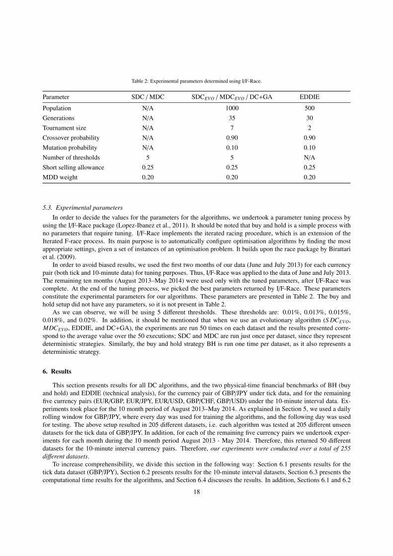
Table 2: Experimental parameters determined using I/F-Race.

Parameter SDC / MDC SDCEVO / MDCEVO / DC+GA EDDIE

Population N/A 1000 500Generations N/A 35 30Tournament size N/A 7 2Crossover probability N/A 0.90 0.90Mutation probability N/A 0.10 0.10Number of thresholds 5 5 N/AShort selling allowance 0.25 0.25 0.25MDD weight 0.20 0.20 0.20

5.3. Experimental parameters

In order to decide the values for the parameters for the algorithms, we undertook a parameter tuning process byusing the I/F-Race package (Lopez-Ibanez et al., 2011). It should be noted that buy and hold is a simple process withno parameters that require tuning. I/F-Race implements the iterated racing procedure, which is an extension of theIterated F-race process. Its main purpose is to automatically configure optimisation algorithms by finding the mostappropriate settings, given a set of instances of an optimisation problem. It builds upon the race package by Birattariet al. (2009).

In order to avoid biased results, we used the first two months of our data (June and July 2013) for each currencypair (both tick and 10-minute data) for tuning purposes. Thus, I/F-Race was applied to the data of June and July 2013.The remaining ten months (August 2013–May 2014) were used only with the tuned parameters, after I/F-Race wascomplete. At the end of the tuning process, we picked the best parameters returned by I/F-Race. These parametersconstitute the experimental parameters for our algorithms. These parameters are presented in Table 2. The buy andhold setup did not have any parameters, so it is not present in Table 2.

As we can observe, we will be using 5 different thresholds. These thresholds are: 0.01%, 0.013%, 0.015%,0.018%, and 0.02%. In addition, it should be mentioned that when we use an evolutionary algorithm (S DCEVO,MDCEVO, EDDIE, and DC+GA), the experiments are run 50 times on each dataset and the results presented corre-spond to the average value over the 50 executions; SDC and MDC are run just once per dataset, since they representdeterministic strategies. Similarly, the buy and hold strategy BH is run one time per dataset, as it also represents adeterministic strategy.

6. Results

This section presents results for all DC algorithms, and the two physical-time financial benchmarks of BH (buyand hold) and EDDIE (technical analysis), for the currency pair of GBP/JPY under tick data, and for the remainingfive currency pairs (EUR/GBP, EUR/JPY, EUR/USD, GBP/CHF, GBP/USD) under the 10-minute interval data. Ex-periments took place for the 10 month period of August 2013–May 2014. As explained in Section 5, we used a dailyrolling window for GBP/JPY, where every day was used for training the algorithms, and the following day was usedfor testing. The above setup resulted in 205 different datasets, i.e. each algorithm was tested at 205 different unseendatasets for the tick data of GBP/JPY. In addition, for each of the remaining five currency pairs we undertook exper-iments for each month during the 10 month period August 2013 - May 2014. Therefore, this returned 50 differentdatasets for the 10-minute interval currency pairs. Therefore, our experiments were conducted over a total of 255different datasets.

To increase comprehensibility, we divide this section in the following way: Section 6.1 presents results for thetick data dataset (GBP/JPY), Section 6.2 presents results for the 10-minute interval datasets, Section 6.3 presents thecomputational time results for the algorithms, and Section 6.4 discusses the results. In addition, Sections 6.1 and 6.2

18

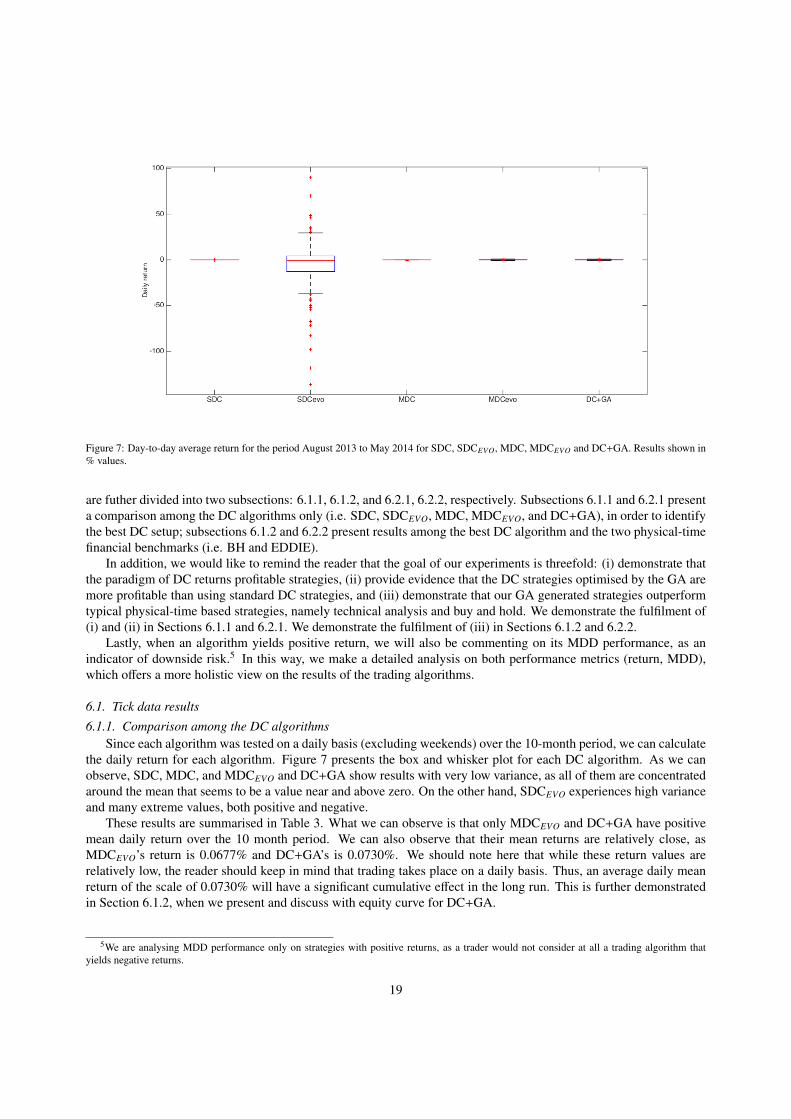
Figure 7: Day-to-day average return for the period August 2013 to May 2014 for SDC, SDCEVO, MDC, MDCEVO and DC+GA. Results shown in% values.

are futher divided into two subsections: 6.1.1, 6.1.2, and 6.2.1, 6.2.2, respectively. Subsections 6.1.1 and 6.2.1 presenta comparison among the DC algorithms only (i.e. SDC, SDCEVO, MDC, MDCEVO, and DC+GA), in order to identifythe best DC setup; subsections 6.1.2 and 6.2.2 present results among the best DC algorithm and the two physical-timefinancial benchmarks (i.e. BH and EDDIE).

In addition, we would like to remind the reader that the goal of our experiments is threefold: (i) demonstrate thatthe paradigm of DC returns profitable strategies, (ii) provide evidence that the DC strategies optimised by the GA aremore profitable than using standard DC strategies, and (iii) demonstrate that our GA generated strategies outperformtypical physical-time based strategies, namely technical analysis and buy and hold. We demonstrate the fulfilment of(i) and (ii) in Sections 6.1.1 and 6.2.1. We demonstrate the fulfilment of (iii) in Sections 6.1.2 and 6.2.2.

Lastly, when an algorithm yields positive return, we will also be commenting on its MDD performance, as anindicator of downside risk.5 In this way, we make a detailed analysis on both performance metrics (return, MDD),which offers a more holistic view on the results of the trading algorithms.

6.1. Tick data results

6.1.1. Comparison among the DC algorithmsSince each algorithm was tested on a daily basis (excluding weekends) over the 10-month period, we can calculate

the daily return for each algorithm. Figure 7 presents the box and whisker plot for each DC algorithm. As we canobserve, SDC, MDC, and MDCEVO and DC+GA show results with very low variance, as all of them are concentratedaround the mean that seems to be a value near and above zero. On the other hand, SDCEVO experiences high varianceand many extreme values, both positive and negative.

These results are summarised in Table 3. What we can observe is that only MDCEVO and DC+GA have positivemean daily return over the 10 month period. We can also observe that their mean returns are relatively close, asMDCEVO’s return is 0.0677% and DC+GA’s is 0.0730%. We should note here that while these return values arerelatively low, the reader should keep in mind that trading takes place on a daily basis. Thus, an average daily meanreturn of the scale of 0.0730% will have a significant cumulative effect in the long run. This is further demonstratedin Section 6.1.2, when we present and discuss with equity curve for DC+GA.

5We are analysing MDD performance only on strategies with positive returns, as a trader would not consider at all a trading algorithm thatyields negative returns.

19

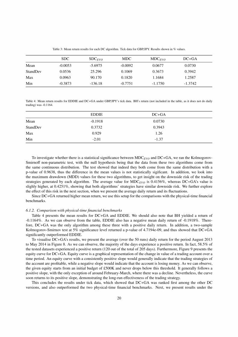
Table 3: Mean return results for each DC algorithm. Tick data for GBP/JPY. Results shown in % values.

SDC SDCEVO MDC MDCEVO DC+GA

Mean -0.0053 -5.6975 -0.0092 0.0677 0.0730StandDev 0.0536 25.296 0.1069 0.3673 0.3942Max 0.0963 90.170 0.1820 1.1684 1.2587Min -0.3873 -136.18 -0.7751 -1.1750 -1.3742

Table 4: Mean return results for EDDIE and DC+GA under GBP/JPY’s tick data. BH’s return (not included in the table, as it does not do dailytrading) was -0.1164.

EDDIE DC+GA

Mean -0.1918 0.0730StandDev 0.3732 0.3943Max 0.929 1.26Min -2.01 -1.37

To investigate whether there is a statistical significance between MDCEVO and DC+GA, we ran the Kolmogorov-Smirnoff non-parametric test, with the null hypothesis being that the data from these two algorithms come fromthe same continuous distribution. The test showed that indeed they both come from the same distribution with ap-value of 0.9638, thus the difference in the mean values is not statistically sigificant. In addition, we look intothe maximum drawdown (MDD) values for these two algorithms, to get insight on the downside risk of the tradingstrategies generated by each algorithm. The average value for MDCEVO is 0.4156%, whereas DC+GA’s value isslighly higher, at 0.4251%, showing that both algorithms’ strategies have similar downside risk. We further explorethe effect of this risk in the next section, when we present the average daily return and its fluctuations.

Since DC+GA returned higher mean return, we use this setup for the comparisons with the physical-time financialbenchmarks.

6.1.2. Comparison with physical-time financial benchmarksTable 4 presents the mean results for DC+GA and EDDIE. We should also note that BH yielded a return of

-0.1164%. As we can observe from the table, EDDIE also has a negative mean daily return of -0.1918%. There-fore, DC+GA was the only algorithm among these three with a positive daily return. In addition, a two-sampleKolmogorov-Smirnov test at 5% significance level returned a p-value of 4.7194e-09, and thus showed that DC+GAsignificantly outperformed EDDIE.

To visualise DC+GA’s results, we present the average (over the 50 runs) daily return for the period August 2013to May 2014 in Figure 8. As we can observe, the majority of the days experience a positive return. In fact, 58.5% ofthe tested datasets experienced a positive return (120 out of the total of 205 days). Furthermore, Figure 9 presents theequity curve for DC+GA. Equity curve is a graphical representation of the change in value of a trading account over atime period. An equity curve with a consistently positive slope would generally indicate that the trading strategies ofthe account are profitable, while a negative slope would indicate that the account is losing money. As we can observe,the given equity starts from an initial budget of £500K and never drops below this threshold. It generally follows apositive slope, with the only exception of around February-March, where there was a decline. Nevertheless, the curvesoon returns to its positive slope, demonstrating the long-run effectiveness of the trading strategy.

This concludes the results under tick data, which showed that DC+GA was ranked first among the other DCversions, and also outperformed the two physical-time financial benchmarks. Next, we present results under the

20

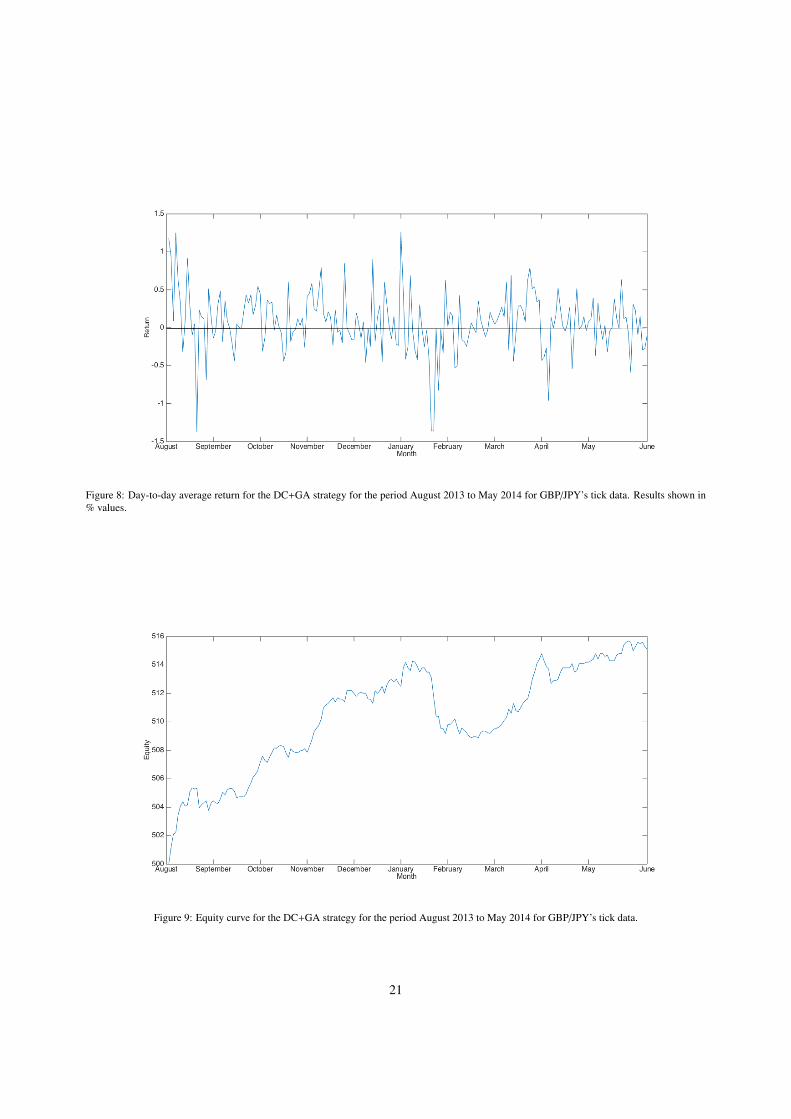
Figure 8: Day-to-day average return for the DC+GA strategy for the period August 2013 to May 2014 for GBP/JPY’s tick data. Results shown in% values.

Figure 9: Equity curve for the DC+GA strategy for the period August 2013 to May 2014 for GBP/JPY’s tick data.

21

10-minute interval data.

6.2. 10-minute interval data results

This section presents results for the 10-minute interval data for the five currency pairs: EUR/GBP, EUR/JPY,EUR/USD, GBP/CHF, and GBP/USD. We start again by presenting results for the DC algorithms only, in Section6.2.1. After identifying the best DC setup, we move on to Section 6.2.2, where we compare this best DC setup withBH and EDDIE.

6.2.1. Comparison among the DC algorithmsTable 5 presents the return results for each month, for each DC algorithm, under the 10-minute interval data, for

each currency pair. Overall, each DC algorithm appears to be able to show positive returns for each currency pair.SDC and SDCEVO are the two algorithms with the highest frequency of positive returns. Out of the 10 months testedper currency pair, SDC had 7 positive returns for EUR/GBP, 6 positive returns for EUR/JPY, 7 positive returns forEUR/USD, 5 positive returns for GBP/CHF, and 3 positive returns for GBP/USD. Similarly, SDCEVO’s number ofpositive returns were 6, 5, 6, 6, and 4.

Table 6 summarises these results. In terms of currency pairs, it appears that EUR/GBP is the easiest to predict,as all algorithms showed non-negative returns. On the other hand, all other currency pairs had two to three currencypairs with negative returns. Overall, SDC and MDC experience again, as with the tick data, a negative mean return.On the other hand, SDCEVO, MDCEVO and DC+GA experience positive mean returns, with values close to each other(0.01064%, 0.00875%, and 0.01046%). It thus appears that these three algorithms have similar performance. Onceagain, we would like to note that while these returns appear to be low, their cumulative effect can be much higherwhen trading over all 50 datasets available for the 10-minute interval data.

To further investigate the algorithms’ performance, we applied Friedman’s non-parametric statistical test to com-pare multiple algorithms. We present the results in Table 7. For each algorithm, the table shows the average rankaccording to the Friedman test (first column), and the adjusted p-value of the statistical test when that algorithm’saverage rank is compared to the average rank of the algorithm with the best rank (control algorithm) according tothe Hommel post-hoc test (second column) (Demšar, 2006; García & Herrera, 2008). As we can observe from theFriedman test, there is no statistical significance between SDCEVO and DC+GA at the α = 0.05 level. Also, there isno statistical significance between SDCEVO and MDCEVO at the α = 0.05 level, but there is a statistical significance atthe α = 0.10 level.

Lastly, we compare the MDD results over the three algorithms that yielded positive mean return (i.e., SDCEVO,MDCEVO, and DC+GA). DC+GA and MDCEVO have the lowest mean MDD values, 0.03789% and 0.03308%, re-spectively; on the other hand, SDCEVO’s mean MDD value is higher, at 0.05251%. Overall, all algorithms showedvery low MDD values. One interesting observation that can be made is that while SDCEVO returned the highest meanreturn, as we saw in Table 6, it also returned more volatile trading strategies. This is mainly because of the muchhigher MDD value for EUR/JPY in Table 8 (0.22863% for SDCEVO, against 0.12386% and 0.14274% for MDCEVO

and DC+GA, respectively). Nevertheless, since SDCEVO ranked first in terms of mean return, we are going to beusing it with the comparisons with the physical-time financial benchmarks.

6.2.2. Comparison with physical-time financial benchmarksTable 9 presents the mean return for EDDIE and SDCEVO under the 10-minute interval datasets (for completeness,

we also present the month-by-month return results in the Appendix in Table A.11.). We should also note that BH’saverage return was 0.01274%. As we can observe, EDDIE has again a negative mean return of -0.00873%; it isalso worth noting that for all five currency pairs EDDIE’s mean return is negative. On the other hand, SDCEVO hasa positive return for three currency pairs: EUR/GBP, EUR/JPY, and EUR/USD. Overall, SDCEVO’s mean return is0.01064%. A two-sample Kolmogorov-Smirnov test for EDDIE and SDCEVO returned a p-value of 0.0560, showingthat there is a statistical significance between these two algorithms at the 10% significance level. However, the factthat EDDIE returned a negative mean return means that it would not be attractive to an investor as a trading algorithm.This leads us to argue that SDCEVO outperforms EDDIE, while it returns a similar average return with BH.

22

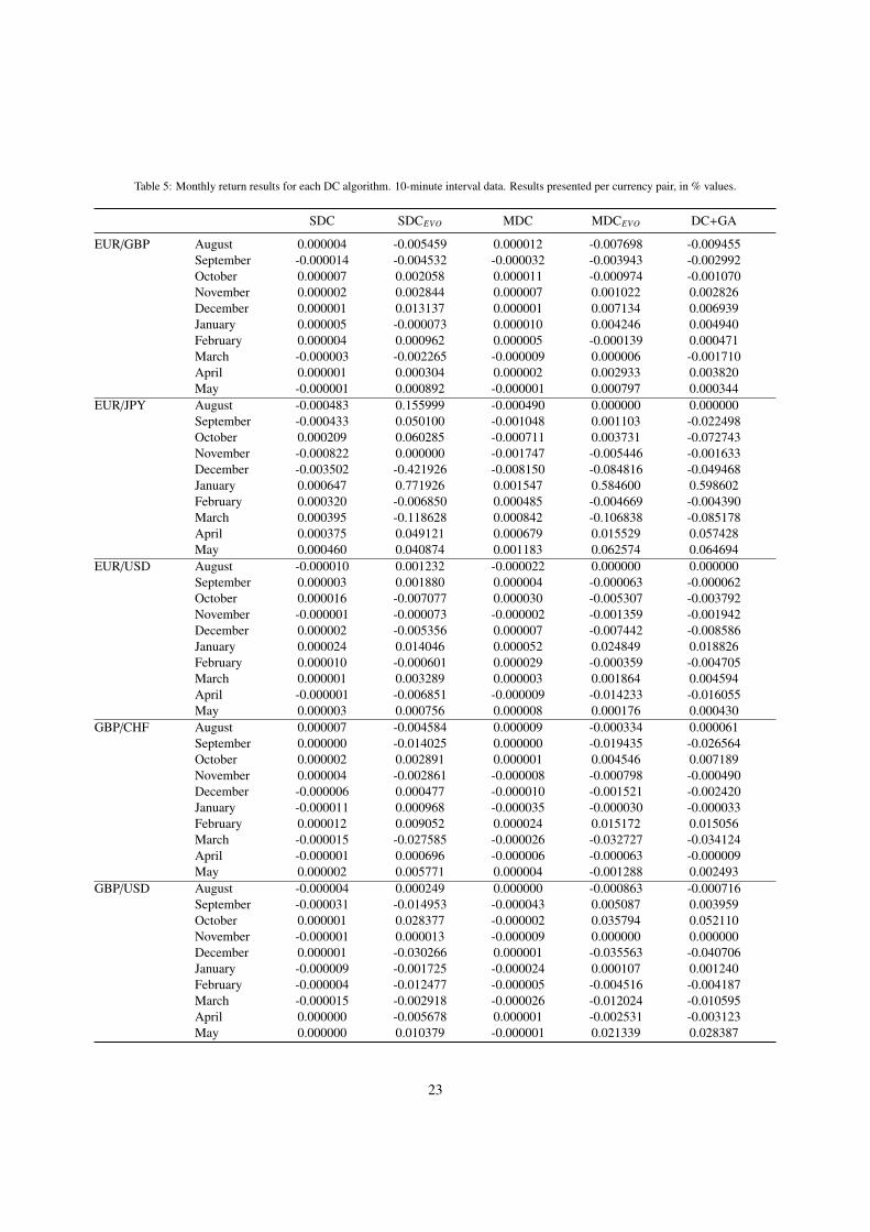
Table 5: Monthly return results for each DC algorithm. 10-minute interval data. Results presented per currency pair, in % values.

SDC SDCEVO MDC MDCEVO DC+GA

EUR/GBP August 0.000004 -0.005459 0.000012 -0.007698 -0.009455September -0.000014 -0.004532 -0.000032 -0.003943 -0.002992October 0.000007 0.002058 0.000011 -0.000974 -0.001070November 0.000002 0.002844 0.000007 0.001022 0.002826December 0.000001 0.013137 0.000001 0.007134 0.006939January 0.000005 -0.000073 0.000010 0.004246 0.004940February 0.000004 0.000962 0.000005 -0.000139 0.000471March -0.000003 -0.002265 -0.000009 0.000006 -0.001710April 0.000001 0.000304 0.000002 0.002933 0.003820May -0.000001 0.000892 -0.000001 0.000797 0.000344

EUR/JPY August -0.000483 0.155999 -0.000490 0.000000 0.000000September -0.000433 0.050100 -0.001048 0.001103 -0.022498October 0.000209 0.060285 -0.000711 0.003731 -0.072743November -0.000822 0.000000 -0.001747 -0.005446 -0.001633December -0.003502 -0.421926 -0.008150 -0.084816 -0.049468January 0.000647 0.771926 0.001547 0.584600 0.598602February 0.000320 -0.006850 0.000485 -0.004669 -0.004390March 0.000395 -0.118628 0.000842 -0.106838 -0.085178April 0.000375 0.049121 0.000679 0.015529 0.057428May 0.000460 0.040874 0.001183 0.062574 0.064694

EUR/USD August -0.000010 0.001232 -0.000022 0.000000 0.000000September 0.000003 0.001880 0.000004 -0.000063 -0.000062October 0.000016 -0.007077 0.000030 -0.005307 -0.003792November -0.000001 -0.000073 -0.000002 -0.001359 -0.001942December 0.000002 -0.005356 0.000007 -0.007442 -0.008586January 0.000024 0.014046 0.000052 0.024849 0.018826February 0.000010 -0.000601 0.000029 -0.000359 -0.004705March 0.000001 0.003289 0.000003 0.001864 0.004594April -0.000001 -0.006851 -0.000009 -0.014233 -0.016055May 0.000003 0.000756 0.000008 0.000176 0.000430

GBP/CHF August 0.000007 -0.004584 0.000009 -0.000334 0.000061September 0.000000 -0.014025 0.000000 -0.019435 -0.026564October 0.000002 0.002891 0.000001 0.004546 0.007189November 0.000004 -0.002861 -0.000008 -0.000798 -0.000490December -0.000006 0.000477 -0.000010 -0.001521 -0.002420January -0.000011 0.000968 -0.000035 -0.000030 -0.000033February 0.000012 0.009052 0.000024 0.015172 0.015056March -0.000015 -0.027585 -0.000026 -0.032727 -0.034124April -0.000001 0.000696 -0.000006 -0.000063 -0.000009May 0.000002 0.005771 0.000004 -0.001288 0.002493

GBP/USD August -0.000004 0.000249 0.000000 -0.000863 -0.000716September -0.000031 -0.014953 -0.000043 0.005087 0.003959October 0.000001 0.028377 -0.000002 0.035794 0.052110November -0.000001 0.000013 -0.000009 0.000000 0.000000December 0.000001 -0.030266 0.000001 -0.035563 -0.040706January -0.000009 -0.001725 -0.000024 0.000107 0.001240February -0.000004 -0.012477 -0.000005 -0.004516 -0.004187March -0.000015 -0.002918 -0.000026 -0.012024 -0.010595April 0.000000 -0.005678 0.000001 -0.002531 -0.003123May 0.000000 0.010379 -0.000001 0.021339 0.028387

23

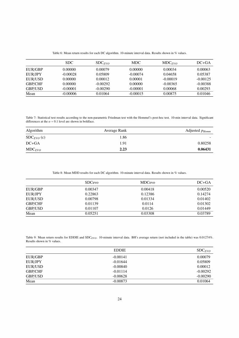
Table 6: Mean return results for each DC algorithm. 10-minute interval data. Results shown in % values.

SDC SDCEVO MDC MDCEVO DC+GA

EUR/GBP 0.00000 0.00079 0.00000 0.00034 0.00063EUR/JPY -0.00028 0.05809 -0.00074 0.04658 0.05387EUR/USD 0.00000 0.00012 0.00001 -0.00019 -0.00125GBP/CHF 0.00000 -0.00292 0.00000 -0.00365 -0.00388GBP/USD -0.00001 -0.00290 -0.00001 0.00068 0.00293Mean -0.00006 0.01064 -0.00015 0.00875 0.01046

Table 7: Statistical test results according to the non-parametric Friedman test with the Hommel’s post-hoc test. 10-min interval data. Significantdifferences at the α = 0.1 level are shown in boldface.

Algorithm Average Rank Adjusted pHomm

SDCEVO (c) 1.86 -DC+GA 1.91 0.80258MDCEVO 2.23 0.06431

Table 8: Mean MDD results for each DC algorithm. 10-minute interval data. Results shown in % values.

SDCevo MDCevo DC+GA

EUR/GBP 0.00347 0.00418 0.00520EUR/JPY 0.22863 0.12386 0.14274EUR/USD 0.00798 0.01334 0.01402GBP/CHF 0.01139 0.0114 0.01302GBP/USD 0.01107 0.0126 0.01449Mean 0.05251 0.03308 0.03789

Table 9: Mean return results for EDDIE and SDCEVO. 10-minute interval data. BH’s average return (not included in the table) was 0.01274%.Results shown in % values.

EDDIE SDCEVO

EUR/GBP -0.00141 0.00079EUR/JPY -0.01644 0.05809EUR/USD -0.00840 0.00012GBP/CHF -0.01114 -0.00292GBP/USD -0.00628 -0.00290Mean -0.00873 0.01064

24

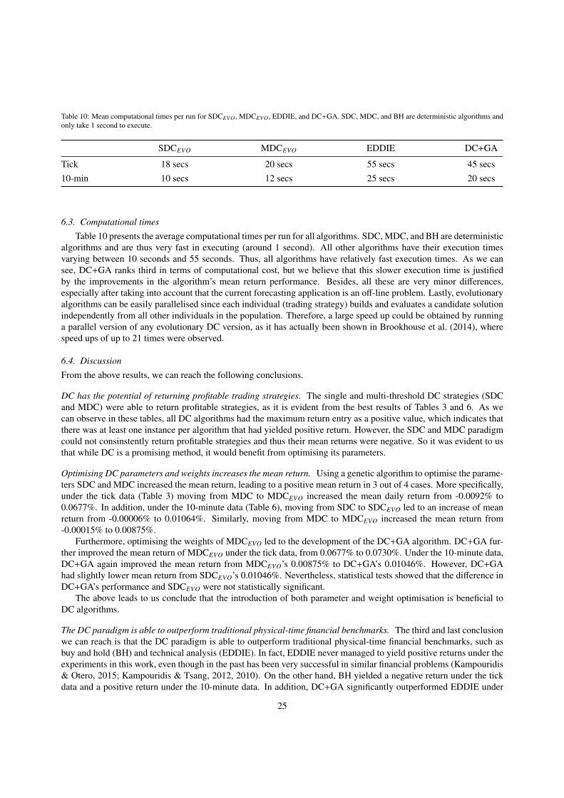
Table 10: Mean computational times per run for SDCEVO, MDCEVO, EDDIE, and DC+GA. SDC, MDC, and BH are deterministic algorithms andonly take 1 second to execute.

SDCEVO MDCEVO EDDIE DC+GA

Tick 18 secs 20 secs 55 secs 45 secs10-min 10 secs 12 secs 25 secs 20 secs

6.3. Computational times

Table 10 presents the average computational times per run for all algorithms. SDC, MDC, and BH are deterministicalgorithms and are thus very fast in executing (around 1 second). All other algorithms have their execution timesvarying between 10 seconds and 55 seconds. Thus, all algorithms have relatively fast execution times. As we cansee, DC+GA ranks third in terms of computational cost, but we believe that this slower execution time is justifiedby the improvements in the algorithm’s mean return performance. Besides, all these are very minor differences,especially after taking into account that the current forecasting application is an off-line problem. Lastly, evolutionaryalgorithms can be easily parallelised since each individual (trading strategy) builds and evaluates a candidate solutionindependently from all other individuals in the population. Therefore, a large speed up could be obtained by runninga parallel version of any evolutionary DC version, as it has actually been shown in Brookhouse et al. (2014), wherespeed ups of up to 21 times were observed.

6.4. Discussion

From the above results, we can reach the following conclusions.

DC has the potential of returning profitable trading strategies. The single and multi-threshold DC strategies (SDCand MDC) were able to return profitable strategies, as it is evident from the best results of Tables 3 and 6. As wecan observe in these tables, all DC algorithms had the maximum return entry as a positive value, which indicates thatthere was at least one instance per algorithm that had yielded positive return. However, the SDC and MDC paradigmcould not consinstently return profitable strategies and thus their mean returns were negative. So it was evident to usthat while DC is a promising method, it would benefit from optimising its parameters.

Optimising DC parameters and weights increases the mean return. Using a genetic algorithm to optimise the parame-ters SDC and MDC increased the mean return, leading to a positive mean return in 3 out of 4 cases. More specifically,under the tick data (Table 3) moving from MDC to MDCEVO increased the mean daily return from -0.0092% to0.0677%. In addition, under the 10-minute data (Table 6), moving from SDC to SDCEVO led to an increase of meanreturn from -0.00006% to 0.01064%. Similarly, moving from MDC to MDCEVO increased the mean return from-0.00015% to 0.00875%.

Furthermore, optimising the weights of MDCEVO led to the development of the DC+GA algorithm. DC+GA fur-ther improved the mean return of MDCEVO under the tick data, from 0.0677% to 0.0730%. Under the 10-minute data,DC+GA again improved the mean return from MDCEVO’s 0.00875% to DC+GA’s 0.01046%. However, DC+GAhad slightly lower mean return from SDCEVO’s 0.01046%. Nevertheless, statistical tests showed that the difference inDC+GA’s performance and SDCEVO were not statistically significant.

The above leads to us conclude that the introduction of both parameter and weight optimisation is beneficial toDC algorithms.

The DC paradigm is able to outperform traditional physical-time financial benchmarks. The third and last conclusionwe can reach is that the DC paradigm is able to outperform traditional physical-time financial benchmarks, such asbuy and hold (BH) and technical analysis (EDDIE). In fact, EDDIE never managed to yield positive returns under theexperiments in this work, even though in the past has been very successful in similar financial problems (Kampouridis& Otero, 2015; Kampouridis & Tsang, 2012, 2010). On the other hand, BH yielded a negative return under the tickdata and a positive return under the 10-minute data. In addition, DC+GA significantly outperformed EDDIE under

25

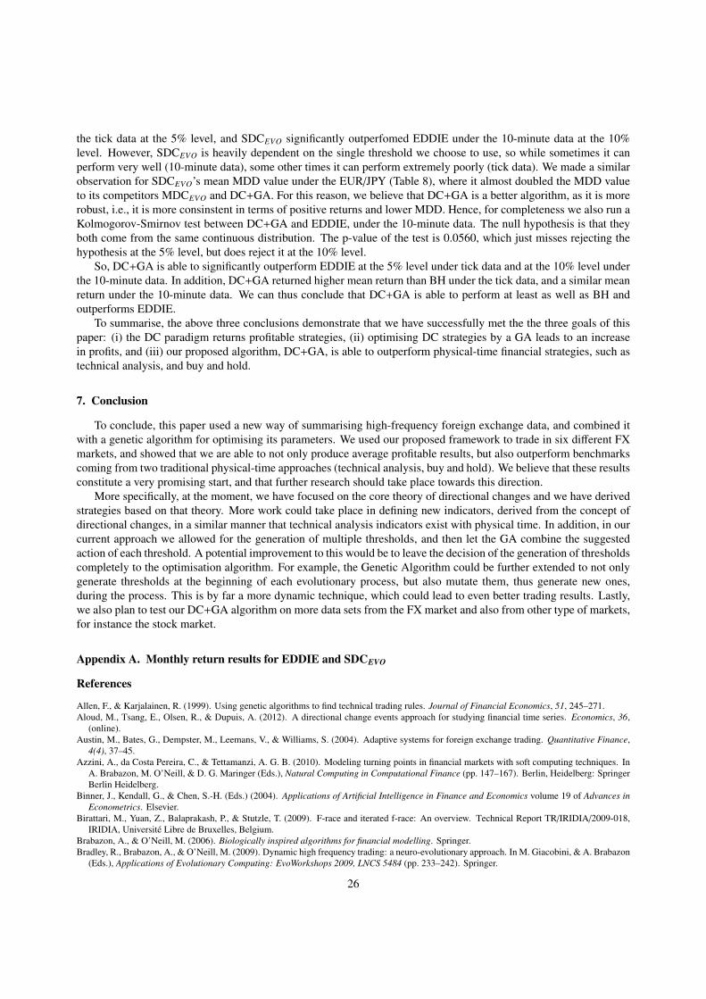
the tick data at the 5% level, and SDCEVO significantly outperfomed EDDIE under the 10-minute data at the 10%level. However, SDCEVO is heavily dependent on the single threshold we choose to use, so while sometimes it canperform very well (10-minute data), some other times it can perform extremely poorly (tick data). We made a similarobservation for SDCEVO’s mean MDD value under the EUR/JPY (Table 8), where it almost doubled the MDD valueto its competitors MDCEVO and DC+GA. For this reason, we believe that DC+GA is a better algorithm, as it is morerobust, i.e., it is more consinstent in terms of positive returns and lower MDD. Hence, for completeness we also run aKolmogorov-Smirnov test between DC+GA and EDDIE, under the 10-minute data. The null hypothesis is that theyboth come from the same continuous distribution. The p-value of the test is 0.0560, which just misses rejecting thehypothesis at the 5% level, but does reject it at the 10% level.

So, DC+GA is able to significantly outperform EDDIE at the 5% level under tick data and at the 10% level underthe 10-minute data. In addition, DC+GA returned higher mean return than BH under the tick data, and a similar meanreturn under the 10-minute data. We can thus conclude that DC+GA is able to perform at least as well as BH andoutperforms EDDIE.

To summarise, the above three conclusions demonstrate that we have successfully met the the three goals of thispaper: (i) the DC paradigm returns profitable strategies, (ii) optimising DC strategies by a GA leads to an increasein profits, and (iii) our proposed algorithm, DC+GA, is able to outperform physical-time financial strategies, such astechnical analysis, and buy and hold.

7. Conclusion

To conclude, this paper used a new way of summarising high-frequency foreign exchange data, and combined itwith a genetic algorithm for optimising its parameters. We used our proposed framework to trade in six different FXmarkets, and showed that we are able to not only produce average profitable results, but also outperform benchmarkscoming from two traditional physical-time approaches (technical analysis, buy and hold). We believe that these resultsconstitute a very promising start, and that further research should take place towards this direction.

More specifically, at the moment, we have focused on the core theory of directional changes and we have derivedstrategies based on that theory. More work could take place in defining new indicators, derived from the concept ofdirectional changes, in a similar manner that technical analysis indicators exist with physical time. In addition, in ourcurrent approach we allowed for the generation of multiple thresholds, and then let the GA combine the suggestedaction of each threshold. A potential improvement to this would be to leave the decision of the generation of thresholdscompletely to the optimisation algorithm. For example, the Genetic Algorithm could be further extended to not onlygenerate thresholds at the beginning of each evolutionary process, but also mutate them, thus generate new ones,during the process. This is by far a more dynamic technique, which could lead to even better trading results. Lastly,we also plan to test our DC+GA algorithm on more data sets from the FX market and also from other type of markets,for instance the stock market.

Appendix A. Monthly return results for EDDIE and SDCEVO

References

Allen, F., & Karjalainen, R. (1999). Using genetic algorithms to find technical trading rules. Journal of Financial Economics, 51, 245–271.Aloud, M., Tsang, E., Olsen, R., & Dupuis, A. (2012). A directional change events approach for studying financial time series. Economics, 36,

(online).Austin, M., Bates, G., Dempster, M., Leemans, V., & Williams, S. (2004). Adaptive systems for foreign exchange trading. Quantitative Finance,

4(4), 37–45.Azzini, A., da Costa Pereira, C., & Tettamanzi, A. G. B. (2010). Modeling turning points in financial markets with soft computing techniques. In

A. Brabazon, M. O’Neill, & D. G. Maringer (Eds.), Natural Computing in Computational Finance (pp. 147–167). Berlin, Heidelberg: SpringerBerlin Heidelberg.

Binner, J., Kendall, G., & Chen, S.-H. (Eds.) (2004). Applications of Artificial Intelligence in Finance and Economics volume 19 of Advances inEconometrics. Elsevier.

Birattari, M., Yuan, Z., Balaprakash, P., & Stutzle, T. (2009). F-race and iterated f-race: An overview. Technical Report TR/IRIDIA/2009-018,IRIDIA, Université Libre de Bruxelles, Belgium.

Brabazon, A., & O’Neill, M. (2006). Biologically inspired algorithms for financial modelling. Springer.Bradley, R., Brabazon, A., & O’Neill, M. (2009). Dynamic high frequency trading: a neuro-evolutionary approach. In M. Giacobini, & A. Brabazon

(Eds.), Applications of Evolutionary Computing: EvoWorkshops 2009, LNCS 5484 (pp. 233–242). Springer.

26

Table A.11: Monthly return results for EDDIE and SDCEVO. 10-minute interval data. Results presented per currency pair. Results shown in %values.

EDDIE SDCEVO

EUR/GBP August 0.004458 -0.005459September 0.005456 -0.004532October -0.013644 0.002058November 0.006171 0.002844December -0.011072 0.013137January -0.010316 -0.000073February -0.001960 0.000962March 0.007997 -0.002265April 0.000799 0.000304May -0.002026 0.000892

EUR/JPY August -0.513460 0.155999September -0.170211 0.050100October -0.088246 0.060285November 0.101843 0.000000December 0.613728 -0.421926January -0.548754 0.771926February 0.033461 -0.006850March 0.400234 -0.118628April 0.048707 0.049121May -0.041675 0.040874

EUR/USD August -0.026099 0.001232September -0.004848 0.001880October -0.053083 -0.007077November 0.004349 -0.000073December -0.0004962 -0.005356January -0.008512 0.014046February 0.011698 -0.000601March -0.000885 0.003289April -0.006766 -0.006851May 0.000674 0.000756

GBP/CHF August -0.019175 -0.004584September 0.002983 -0.014025October -0.036008 0.002891November -0.030220 -0.002861December -0.019675 0.000477January 0.007053 0.000968February 0.009592 0.009052March -0.008943 -0.027585April -0.002353 0.000696May -0.014646 0.005771

GBP/USD August 0.000832 0.000249September -0.009259 -0.014953October 0.002542 0.028377November 0.001273 0.000013December -0.020717 -0.030266January 0.007417 -0.001725February -0.005826 -0.012477March -0.029045 -0.002918April -0.002988 -0.005678May -0.007080 0.010379

27

Brookhouse, J., Otero, F., & Kampouridis, M. (2014). Working with OpenCL to speed up a genetic programming financial forecasting algorithm:Intial results. In Proceedings of the Companion Publication of the 2014 Annual Conference on Genetic and Evolutionary Computation (GECCO)(pp. 1117–1124). ACM.

Cervelló-Royo, R., Guijarro, F., & Michniuk, K. (2015). Stock market trading rule based on pattern recognition and technical analysis: Forecastingthe DJIA index with intraday data. Expert Systems with Applications, 4 (14), 5963–5975.

Chen, S.-H. (2002). Genetic Algorithms and Genetic Programming in Computational Finance. Springer-Verlag New York, LLC.Chen, T. L., & Chen, F. Y. (2016). An intelligent pattern recognition model for supporting investment decisions in stock market. Information

Sciences, 346, 261–274.Chiang, W. C., Enke, D., Wu, T., & Wang, R. (2016). An adaptive stock index trading decision support system. Expert Systems with Applications,

59, 195–207.Chourmouziadis, K., & Chatzoglou, P. D. (2016). An intelligent short term stock trading fuzzy system for assisting investors in portfolio manage-

ment. Expert Systems with Applications, 43, 298–311.Demšar, J. (2006). Statistical Comparisons of Classifiers over Multiple Data Sets. Journal of Machine Learning Research, 7, 1–30.Dupuis, A., & Olsen, R. (2012). High frequency finance: using scaling laws to build trading models. In J. James (Ed.), Handbook of exchange

rates chapter 20. Wiley, NJ, USA.Evans, C., Pappas, K., & Xhafa, F. (2013). Utilizing artificial neural networks and genetic algorithms to build an algo-trading model for intra-day

foreign exchange speculation. Mathematical and Computer Modelling, 58, 1249–1266.García, S., & Herrera, F. (2008). An Extension on “Statistical Comparisons of Classifiers over Multiple Data Sets” for all Pairwise Comparisons.

Journal of Machine Learning Research, 9, 2677–2694.Garcia-Almanza, A., Alexandrova-Kabadjova, B., & Martinez-Jaramillo, S. (2013). Bankruptcy prediction for banks: An artificial intelligence

approach to improve understandability. In X.-S. Yang (Ed.), Artificial Intelligence, Evolutionary Computing and Metaheuristics (pp. 633–656).Springer Berlin Heidelberg volume 427 of Studies in Computational Intelligence.

Glattfelder, J., Dupuis, A., & Olsen, R. (2011). Patterns in high-frequency FX data: Discovery of 12 empirical scaling laws. Quantitative Finance,11 (4), 599–614.

Godlberg, D. (1989). Genetic Algorithms in Search Optimisation and Machine Learning. Addison-Wesley.Gypteau, J., Otero, F. E., & Kampouridis, M. (2015). Generating directional change based trading strategies with genetic programming. In M. A.

Mora, & G. Squillero (Eds.), Applications of Evolutionary Computation: 18th European Conference (pp. 267–278). Springer.Hu, Y., Liu, K., Zhang, X., Su, L., Ngai, E., & Liu, M. (2015). Application of evolutionary computation for rule discovery in stock algorithmic

trading. Appl. Soft Comput., 36, 534–551.International Monetary Fund (2009). Global financial stability report. https://www.imf.org/external/pubs/ft/gfsr/2009/01/pdf/text.pdf.Jaisinghani, D. (2016). An empirical test of calendar anomalies for the indian securities markets. South Asian Journal of Global Business Research,

5 (1), 53–84.Kampouridis, M., & Otero, F. E. B. (2015). Heuristic procedures for improving the predictability of a genetic programming financial forecasting

algorithm. Soft Computing, (pp. 1–16).Kampouridis, M., & Tsang, E. (2010). EDDIE for investment opportunities forecasting: Extending the search space of the GP. In Proceedings of

the IEEE World Congress on Computational Intelligence (pp. 2019–2026). Barcelona, Spain.Kampouridis, M., & Tsang, E. (2012). Investment opportunities forecasting: Extending the grammar of a GP-based tool. Int. Journal of Computa-

tional Intelligence Systems, 5, 530–541.Kim, Y., & Enke, D. (2016). Developing a rule change trading system for the futures market using rough set analysis. Expert Systems with

Applications, 59, 165–173.Koza, J. (1992). Genetic Programming: On the programming of computers by means of natural selection. Cambridge, MA: MIT Press.Kwon, Y.-K., & Moon, B.-R. (2007). A hybrid neurogenetic approach for stock forecasting. IEEE Transactions on Neural Networks, 18, 851–864.Lopez-Ibanez, M., Dubois-Lacoste, J., Stutzle, T., & Birattari, M. (2011). The irace package, iterated race for automatic algorithm configuration.

Technical Report TR/IRIDIA/2011-004, IRIDIA, Université Libre de Bruxelles, Belgium.Mani, S. (1996). Financial forecasting using genetic algorithms. Applied Artificial Intelligence, 10, 543–566.Martinez-Jaramillo, S. (2007). Artificial Financial Markets: An agent-based Approach to Reproduce Stylized Facts and to study the Red Queen

Effect. Ph.D. thesis CFFEA, University of Essex.Michalewicz, Z. (2002). Genetic algorithms + data structures = evolution programs. Springer.Mitchell, M. (1996). An Introduction to Genetic Algorithms. MIT Press, Cambridge, MA.Olsen, R. B., Muller, U. A., Dacorogna, M. M., Pictet, O. V., Dave, R. R., & Guillaume, D. M. (1997). From the bird’s eye to the microschope: A

survey of new stylized facts of the intra-day foreign exchange markets. Finance and Stochastics, 1 (2), 95–129.Tsang, E., Markose, S., & Er, H. (2005). Chance discovery in stock index option and future arbitrage. New Mathematics and Natural Computation,

World Scientific, 1(3), 435–447.Tsang, E., & Martinez-Jaramillo, S. (2004). Computational finance. IEEE Computational Intelligence Society Newsletter, (pp. 3–8).Tsang, E., Tao, R., Serguieva, A., & Ma, S. (2016). Profiling high-frequency equity price movements in directional changes. Quantitative Finance,

2016, (online).

28