Exact and approximation algorithms for

the expanding search problem

Ben Hermans∗,a, Roel Leusa, and Jannik Matuschkeb

aResearch Center for Operations Research & Business Statistics, KU Leuven,Belgium

bResearch Center for Operations Management, KU Leuven, Belgium

Abstract

Suppose a target is hidden in one of the vertices of an edge-weighted graphaccording to a known probability distribution. The expanding searchproblem asks for a search sequence of the vertices so as to minimize theexpected time for finding the target, where the time for reaching thenext vertex is determined by its distance to the region that was alreadysearched. This problem has numerous applications, such as searching forhidden explosives, mining coal, and disaster relief. In this paper, we de-velop exact algorithms and heuristics, including a branch-and-cut proce-dure, a greedy algorithm with a constant-factor approximation guarantee,and a novel local search procedure based on a spanning tree neighborhood.Computational experiments show that our branch-and-cut procedure out-performs all existing methods for general instances and both heuristicscompute near-optimal solutions with little computational effort.

1 Introduction

The problem of searching a hidden target plays a major role in the daily op-erations of search and rescue teams, intelligence services, and law enforcementagencies. Research and development departments in corporations also face asearch problem when they need to identify a viable product design. One way torepresent the search space is by a graph in which each vertex has a given proba-bility to contain the target and each edge has a length that reflects the distance(cost, time, or a composite measure) to move between the adjacent vertices.We study the problem of a searcher who, starting from a predetermined root,needs to determine how to search the graph in order to minimize the expecteddistance traveled before finding the target.

The traditional paradigm of pathwise search assumes that the searcher canonly continue searching from their current location, which leads to a searchtrajectory that forms a walk in the graph. In this paper, we adopt the alternativeparadigm of expanding search, as introduced by Alpern and Lidbetter (2013).Here, the searcher can proceed from every previously visited vertex and theresulting trajectory forms a tree in the graph. Such a search arises naturally

∗The author is funded by a PhD Fellowship of the Research Foundation – Flanders.

1

arX

iv:1

911.

0895

9v1

[cs

.DM

] 2

0 N

ov 2

019

when the cost to traverse an edge for a second time is negligible compared tothe first traversal. When mining for coal, for example, moving within existingtunnels can occur in time negligible compared to the time needed to dig intoa new site (Alpern and Lidbetter, 2013). Similarly, when securing an area fora hidden explosive, moving within a secured area takes considerably less timethan securing a new location (Angelopoulos et al., 2019).

Another application for the expanding search paradigm follows from thesituation where we want to minimize the weighted average (re)connection timeof a graph’s vertices to its root (Averbakh and Pereira, 2012). In the contextof disaster relief, for example, the vertices could reflect villages, the root anaid center, and the edges road segments that have been destroyed by a naturaldisaster. Edge lengths represent the time necessary to clear the roads and oncea road segment has been cleared, the time to travel over it becomes negligible.The problem then consists in deciding the order in which to clear the roads soas to minimize the weighted reconnection time of all villages to the aid center,where the weighting occurs according to the relative importance of differentvillages. This is equivalent to the expanding search problem if we interpretvertex weights as a measure of relative importance rather than as a probabilitythat the respective vertex contains the target.

Contribution and main findings. In this paper, we study exact and ap-proximation algorithms for the expanding search problem. While a substantialamount of work has been done for the pathwise search problem, research onexpanding search has only emerged relatively recently. In particular, to thebest of our knowledge, no approximation algorithm for the problem has beendeveloped so far. This paper fills this gap by showing how a greedy approachyields a constant-factor approximation algorithm. As a second contribution,we develop a branch-and-cut procedure that finds an optimal expanding searchsequence for instances that were not solved by previous methods. Finally, wealso describe a local search procedure.

Our branch-and-cut procedure relies on a novel mixed integer program forthe expanding search problem that exploits the knowledge of how to solve thespecial case of trees. We build upon the single-machine scheduling literature(Correa and Schulz, 2005) to obtain a linear program that identifies an op-timal search sequence for a given tree, and we embed this formulation in amixed integer program to select an optimal tree within the graph. Inspired bywell-known results for the minimum spanning tree problem, we obtain valid in-equalities that form the basis of our branch-and-cut procedure. Computationalexperiments show that our branch-and-cut procedure outperforms the existingmethods for general instances and that the computational performance greatlydepends on the graph’s density.

The greedy approximation algorithm starts from the intuitive idea that oneprefers to probe groups of nearby vertices with a high probability to containthe object. More specifically, we employ the concept of the search density ofa subtree, defined as the ratio of (i) the total probability mass of all verticesin the subtree and (ii) the total length of all edges in the subtree. Using aproof technique inspired by Feige et al. (2004), we show that a greedy approachof approximating the subtree of maximum search density and then searchingthat tree leads to an 8-approximation algorithm. Computational experiments

2

suggest that, empirically, the greedy approach produces solutions much closerto optimality than the factor eight worst-case guarantee.

Our local search procedure, finally, iteratively improves the current solutionwithin an edge-swap neighborhood based on the spanning tree representationof the search sequence, exploiting our ability to find the optimal search for agiven tree efficiently. We observe that it is crucial to consider all edge swapsin the metric closure of the input graph. We further show that this procedurefinds the optimum when the underlying graph is a cycle. This contrasts with arelated insertion-based local search of Averbakh and Pereira (2012), for whichwe observe that it can perform arbitrarily bad on a cycle. Moreover, our localsearch found the optimum for around 80% of the instances in our computationalexperiment and it exceeded the optimal value by at most 2.15% for the othercases.

Related work. Since the seminal work of Koopman (1956a,b, 1957), searchtheory has grown to a rich area of research; see the books of Alpern and Gal(2003), Stone (2007), Alpern et al. (2013), and Stone et al. (2016) for gen-eral overviews. We focus on the work directly related to the expanding searchproblem, and compare it to previous work on the pathwise search problem.

It has been established that the pathwise search problem is NP-hard (Trum-mel and Weisinger, 1986), even if the underlying graph forms a tree (Sitters,2002). Archer et al. (2008) describe a 7.18-approximation algorithm for theproblem, and Li and Huang (2018) give an exact solution method that also al-lows for multiple searchers. Many of these results exploit the connection betweenthe pathwise search problem and the minimum latency problem, also known asthe traveling repairman problem, which asks for a tour that visits all verticesand minimizes the sum of arrival times (Afrati et al., 1986). Indeed, the path-wise search problem can be seen as a node-weighted version of the minimumlatency problem (Koutsoupias et al., 1996; Ausiello et al., 2000).

Considerably less work has been done for the expanding search problem.Averbakh and Pereira (2012) show that the problem is NP-hard in general anddevelop exact solution methods. Averbakh (2012) develops polynomial-time al-gorithms for a more general model that allows for multiple searchers, but onlyfor the special case where the graph is a path. Alpern and Lidbetter (2013)describe a polynomial algorithm for the expanding search problem when theunderlying graph is a tree, and Tan et al. (2019) study both exact and approxi-mation algorithms when there are multiple searchers, again for the special caseof trees. Fokkink et al. (2019), finally, generalize the algorithm of Alpern andLidbetter (2013) to submodular cost and supermodular weight functions. Thisgeneralization, however, does not work for general graphs since the length nec-essary to search a set of vertices is, in general, not a submodular function ofthat set.

Several articles have also studied expanding search games, where an adver-sary, or hider, chooses the target’s location so as to maximize the expected searchtime. This then leads to a zero-sum game between the searcher and hider. Inthis setting, the probability distribution for the target’s location cannot be takenas given, but results from an optimal (mixed) hider strategy. Alpern and Lid-better (2013) solve the game for trees and 2-edge-connected graphs, and Alpernand Lidbetter (2019) describe a method to approximate the game’s value for

3

arbitrary graphs. Angelopoulos et al. (2019) study a related problem where thesearcher wants to minimize the expanding search ratio, defined as the maximumover all vertices of (i) the length that the search needs to reach a vertex and (ii)the shortest path between the root and that vertex. The authors show that theproblem is NP-hard and find constant-factor approximation algorithms.

Overview. After formally defining the expanding search problem in Section 2,we develop our branch-and-cut procedure in Section 3. Next, we describe ourgreedy approximation algorithm and local search in Section 4, and report ourfindings from the computational experiments in Section 5. Finally, we concludeand discuss potential future work in Section 6.

2 Problem statement

Let G = (V,E) be a connected graph with root r ∈ V , a probability pv ∈ [0, 1]associated to each vertex v ∈ V , and a length λe ∈ R>0 to each edge e ∈ E.Denote the number of non-root vertices by n = |V \ r|. We consider onesearcher who has perfect information about the vertex probabilities and edgelengths. Finally, we assume that the target is hidden at exactly one of thenon-root vertices such that pr = 0 and

∑v∈V pv = 1.

We define an expanding search as a sequence of edges σ = (e1, . . . , en) suchthat r ∈ e1 and each edge ek, with k = 1, . . . , n, connects an unvisited vertex toone of the previously visited vertices. Hence, the edges e1, . . . , ek form a tree

in G for every k = 1, . . . , n. Next, denote by λ(σ, v) =∑ki=1 λei the distance

traveled until the search σ = (e1, . . . , en) reaches vertex v ∈ V , where ek is thefirst edge in σ with v ∈ ek. The search cost c(σ) of an expanding search σ,defined as the expected distance traveled before finding the target, then equals

c(σ) =∑v∈V

pvλ(v, σ), (1)

and the expanding search problem asks to find an expanding search that min-imizes this search cost. As mentioned above, Averbakh and Pereira (2012,Theorem 1) have shown that a problem equivalent to the expanding searchproblem is strongly NP-hard. Hence, unless P = NP, no polynomial-time algo-rithm that solves the expanding search problem exists and we need to rely onexponential-time (Section 3) or approximation (Section 4) algorithms.

3 Branch-and-cut procedure

The mixed integer program that forms the base of our branch-and-cut procedureembeds a linear program to determine an optimal search sequence on a given tree(Section 3.1) within a mixed integer program that selects a tree (Section 3.2).We also introduce two classes of valid inequalities to strengthen the formulation(Section 3.3) and show how to separate these valid inequalities (Section 3.4).

3.1 Linear program for trees

If G takes the form of a rooted tree, then the searcher can only probe a vertexv ∈ V \ r if all vertices on the unique path from r to v in the tree have

4

already been searched. Let A denote the set of arcs obtained by directingall edges in the tree so as to reflect these precedence constraints. That is,the set A contains an arc (i, j) for each edge i, j ∈ E such that vertex i isthe immediate predecessor of vertex j in the tree’s unique path from r to j.Several polynomial-time algorithms for the expanding search problem on a treethen arise as a special case of existing methods for sequencing with precedenceconstraints (Sidney, 1975; Monma and Sidney, 1979; Queyranne and Wang,1991; Correa and Schulz, 2005).

Define a decision variable δij for each pair of vertices i, j ∈ V that indicateswhether or not the search visits vertex i before j, and a decision variable zifor each vertex i ∈ V that records the probability that the target has not beenfound before visiting vertex i. Now consider the following linear program.

[LP] min∑

(i,j)∈A

λi,jzj (2)

s.t. δij + δji = 1 ∀ i, j ∈ V , i 6= j (3)

δij + δjk + δki ≥ 1 ∀ i, j, k ∈ V , i 6= j 6= k 6= i (4)

δij = 1 ∀ (i, j) ∈ A (5)

pi +∑

j∈V \i

pjδij = zi ∀ i ∈ V (6)

δij ≥ 0 ∀ i, j ∈ V (7)

To see why this is a correct formulation for the expanding search problem ona tree, suppose first that all variables δij are either zero or one. Constraints (3)then make sure that vertex i is searched either before or after vertex j. Togetherwith Constraints (4) and (5), this also enforces transitivity and the precedenceconstraints (Potts, 1980). Constraints (6), in turn, state that the target has notbeen found before reaching a certain vertex i with a probability equal to thetotal probability mass of all vertices unvisited prior to arriving at that vertex i.The objective function (2), finally, combines the length of each arc with theprobability that the searcher travels through this arc. Correa and Schulz (2005)have shown that a linear program equivalent to [LP], denoted [P-LP] in theirarticle, has an optimal solution with all variables δij either zero or one. Hence,the linear program [LP] provides a correct formulation for the expanding searchproblem on a tree.

3.2 Mixed integer program for general graphs

We keep the notation of the previous section except for A = (i, j), (j, i) : i, j ∈E, which now includes an arc for both possible directions to move over eachedge. We say that the search uses arc (i, j) ∈ A if the searcher travels fromvertex i to vertex j through edge i, j. In addition to the decision variablesused in the linear program [LP], we introduce for each arc (i, j) ∈ A a binarydecision variable xij that indicates whether or not the search uses arc (i, j) and,similarly, a continuous decision variable yij that records the probability thatthe searcher did not find the target before using arc (i, j). The following mixedinteger program then constitutes a valid formulation for the expanding search

5

problem on general graphs.

[MIP] min∑

(i,j)∈A

λi,jyij (8)

s.t. (3), (4), (6), and (7)∑i: (i,j)∈A

xij = 1 ∀ j ∈ V \ r (9)

∑i: (i,j)∈A

yij = zj ∀ j ∈ V \ r (10)

0 ≤ yij ≤ xij ≤ δij ∀ (i, j) ∈ A (11)

xij ∈0, 1 ∀ (i, j) ∈ A (12)

Similarly as before, the objective function (8) combines the length of eachedge with the probability that the searcher travels through that edge. Con-straints (9) state that the search must reach every non-root vertex throughexactly one arc, and Constraints (3), (4) and (11) prevent cycles. Together withConstraints (12), all feasible assignments to the variables (xij)(i,j)∈A thus consti-tute a spanning tree of G with root r. By Constraints (10), the probability thatthe search reaches a vertex equals the total probability with which the searchtravels through an arc leading to that vertex. Combined with Constraints (9)and (11), this implies that for each vertex j ∈ V \ r we have yij = zj if (i, j)is the unique arc reaching vertex j (and thus having xij = 1), and yij = 0otherwise. Hence, the x-variables select a tree, the δ- and z-variables determinean optimal search sequence on this tree, and the y-variables translate this tothe associated search cost.

3.3 Valid inequalities

The main source of weakness for the linear programming (LP) relaxation of[MIP] is that, in the presence of fractional values for the x-variables, there canbe multiple arcs (i, j) leading to the same vertex j with a positive value foryij . The valid inequalities to be discussed in this section attempt to bettercoordinate the value of these y-variables.

The first set of valid inequalities is inspired by the so-called “directed cutmodel” for spanning trees (see e.g. Magnanti and Wolsey, 1995):∑

(i,j)∈C(S)

yij ≥ zk for all k ∈ V \ r and S ⊆ V \ k with r ∈ S. (13)

Here, the directed cut C(S) = (i, j) ∈ A : i ∈ S, j /∈ S collects all arcs startingin S and ending in V \ S. The inequalities are valid because at least one arcin each directed cut C(S) that separates a vertex k from the root should betraveled through with at least the probability to reach this vertex k.

Our second set of valid inequalities is similar to Constraints (13), exceptthat now we directly use the probability parameters (pi)i∈V instead of decisionvariables (zi)i∈V :∑

(i,j)∈C(S)

yij ≥∑i∈V \S

pi for all S ⊆ V with r ∈ S. (14)

6

These inequalities are valid since at least one arc in the directed cut C(S)should be traveled through with a probability equal to the probability massof all vertices outside set S. For the special case where S = V \ j for somej ∈ V \ r, these inequalities can be strengthened to

zj =∑

i: (i,j)∈A

yij ≥ pj + yjk ∀ (j, k) ∈ A. (15)

Indeed, the searcher travels to vertex j with a probability at least the sum ofthe probability that vertex j contains the object and that the searcher travelsthrough arc (j, k).

In the remainder of this paper, we refer to the two classes of Inequalities (13)and (14)-(15) as cuts (C1) and (C2), respectively.

3.4 Separation

Constraints (13) and (14) contain exponentially many inequalities and it istherefore undesirable to include them all. Instead, we embed these inequalitiesin a cutting plane algorithm that iteratively solves the LP relaxation of [MIP],checks whether a violated valid inequality exists and, if so, adds it. This givesrise to a branch-and-cut procedure where we use the cutting plane algorithm tosolve the LP relaxations and branch on whether or not to use an arc.

For both Constraints (13) and (14), we can check whether there is a violatedinequality by solving O(n) minimum cut problems. Let (x?ij , y

?ij)(i,j)∈A, (z?j )j∈V

be a given solution to the LP relaxation and consider the directed graph (V,A) inwhich arc (i, j) ∈ A has capacity y?ij . A violated inequality for Constraints (13)then exists if and only if there is a vertex k ∈ V \ r for which the minimumdirected cut separating r from k has a capacity strictly smaller than z?k. A similarapproach allows to separate Constraints (14), except that now we additionallyintroduce a dummy sink node t in our directed graph and an extra arc (i, t)for each node i ∈ V with capacity pi. Since

∑i∈V \S pi = 1 −

∑i∈S pi for each

S ⊆ V , a violated inequality for Constraints (14) then exists if and only if theminimum directed cut has a capacity strictly smaller than one.

4 Approximation algorithm

If the graph is a star with the root at its center, traveling to a non-root vertex vtakes the same distance λr,v, independently of which vertices have been visitedbefore. A straightforward pairwise interchange argument then shows that it isoptimal to visit the vertices in non-increasing order of the ratio pv/λr,v (Smith,1956). The search density of a subgraph generalizes this idea to subgraphs bytaking the ratio of (i) the total probability mass of all vertices in the subgraphand (ii) the total length of all edges in the subgraph.

Alpern and Lidbetter (2013) have shown that if G is a tree, then there existsan optimal search that starts with searching the edges of a maximum densitysubtree. Although this approach may be suboptimal in general graphs (Alpernand Lidbetter, 2013), we will show that the resulting search cost is at mostfour times the optimal one. The problem of finding a subtree of maximumdensity in a general graph, however, is also strongly NP-hard. We develop a1/2-approximation for this problem (Section 4.1) and show how this leads to an

7

8-approximation for the expanding search problem (Section 4.2). In Section 4.3,finally, we discuss a local search procedure to further improve the sequence foundby the approximation algorithm.

4.1 The maximum density subtree problem

Given an arbitrary graph G′, let V [G′] and E[G′] collect the vertices and edgesof G′, respectively. For a set of vertices V ′ ⊆ V of edges E′ ⊆ E, we usethe notation p(V ′) =

∑v∈V ′ pv and λ(E′) =

∑e∈E′ λe. Let T (G) collect all

subtrees with root r of the graph G and, given a subtree T ∈ T (G), denotep(T ) = p(V [T ]) and λ(T ) = λ(E[T ]). The search density, or simply density, ofa subtree T ∈ T (G) with λ(T ) > 0 is then defined as

ρ(T ) =p(T )

λ(T ),

and the maximum density subtree problem (MDSP) asks to find a tree T ? ∈T (G) that maximizes this density:

ρ? = ρ(T ?) = maxT∈T (G)

ρ(T ).

The MDSP can be solved efficiently by a dynamic program in case G is a tree(Alpern and Lidbetter, 2013), but it is strongly NP-hard in general (Lau et al.,2006, Theorem 8). Kao et al. (2013) describe both exact and approximationalgorithms for different variants of the MDSP, but, to the best of our knowledge,we are the first to develop an approximation algorithm for the MDSP as definedabove.

As a subroutine to our approximation algorithm, we consider a sequence ofinstances for the prize-collecting Steiner tree (PCST) problem. Given a con-nected graph G = (V,E) with root r, edge lengths (λe)e∈E , and vertex penal-ties (p)v∈V , the PCST problem asks to find a tree T ∈ T (G) that minimizesλ(T )+p(V \V [T ]). Goemans and Williamson (1995) have developed an approx-imation algorithm (henceforth called the GW algorithm) for the PCST problemwith the following guarantee:

Theorem 1 (Goemans and Williamson, 1995). The GW algorithm yields a treeT ∈ T (G) with

λ(T ) +

(2− 1

n

)p(V \ V [T ]) ≤

(2− 1

n

)(λ(T ′) + p(V \ V [T ′]))

for each T ′ ∈ T (G).

Our approximation algorithm for the MDSP consists of a parametric searchwhere we iteratively guess a value for the maximum density ρ? and evaluate ourguess by employing the GW-algorithm. In particular, given a constant ε > 0,our parametric search produces a subtree T s ∈ T (G) as follows:

1. Take arbitrary T s ∈ T (G), and initialize α ←(2− 1

n

)p(T s)/λ(T s) and

β ← maxpv/λv,w : v, w ∈ E

2. While β > (1 + ε)α, do

8

(a) ρ← (α+ β)/2

(b) let T be the subtree obtained by applying the GW algorithm ongraph G with lengths (ρλe)e∈E and penalties (pv)v∈V

(c) if(2− 1

n

)p(T ) ≤ ρλ(T ), let β ← ρ; else, let α ←

(2− 1

n

)ρ(T ) and

T s ← T

3. Return T s.

Proposition 1. For each ε > 0, the maximum density ρ? is at most((1 + ε)

(2− 1

n

))times the density ρ(T s) of the tree T s obtained by the parametric search.

Proof. Denote by αi, βi, and T si the values for α, β, and T s at the beginning of

iteration i in the while loop, and let T ? be a tree with maximum density ρ? . Weclaim that for each iteration i ≥ 1 it holds that ρ? ≤ βi and αi =

(2− 1

n

)ρ(T s

i ).Since β ≤ (1 + ε)α after the final iteration, this implies

ρ? ≤ (1 + ε)α = (1 + ε)

(2− 1

n

)ρ(T s),

which would then prove the result.We prove the claim by induction. By definition, α1 =

(2− 1

n

)ρ(T s

1). Sincefor every two sequences a1, . . . , ak and b1, . . . , bk of respectively non-negativeand positive numbers it holds that

maxj=1,...,k

ajbj≥∑kj=1 aj∑kj=1 bj

,

we also have that β1 ≥ ρ?.Next, take an arbitrary iteration i ≥ 1, and assume that βi ≥ ρ? and

αi =(2− 1

n

)ρ(T s

i ). Let T be the subtree obtained by the GW algorithm anddistinguish between two cases. Firstly, if(

2− 1

n

)p(T ) ≤ ρλ(T ),

then adding(2− 1

n

)p(V \ V [T ]) to both sides of this inequality yields that(

2− 1

n

)p(V ) ≤ ρλ(T ) +

(2− 1

n

)p(V \ V [T ]).

Hence, by Theorem 1, we have for each T ′ ∈ T (G) that(2− 1

n

)p(V ) ≤

(2− 1

n

)(ρλ(T ′) + p(V \ V [T ′]))

or, equivalently, that ρλ(T ′) ≥ p(T ′). Thus, our guess ρ for the density wastoo high, and we obtain that βi+1 = ρ ≥ ρ?, while αi+1 = αi and T s

i+1 = T si .

Alternatively, if(2− 1

n

)p(T ) > ρλ(T ), then(

2− 1

n

)p(V ) > ρλ(T ) +

(2− 1

n

)p(V \ V [T ]),

which yields that(2− 1

n

)ρ(T ) > ρ. Thus, our guess ρ for the density was

too low, and we have αi+1 =(2− 1

n

)ρ(T s

i+1) > ρ and βi+1 = βi. Togetherwith the induction hypothesis, we obtain in both cases that ρ? ≤ βi+1 andαi+1 =

(2− 1

n

)ρ(T s

i+1), which proves the claim.

9

As summarized by the next result, by choosing ε = 1/(2n− 1), we obtain a1/2-approximation algorithm for the MDSP. The associated running time con-sists of the one for the GW algorithm multiplied with the number of iterationsin the while loop. In particular, Hegde et al. (2015, Theorem 28) discuss howthe GW algorithm can be implemented to run in time O(|E| log(n) log(M)) and,for every ε > 0, the number of iterations in the while loop is O(log(M/ε)).

Corollary 1. For ε = 1/(2n−1), the parametric search is a 1/2-approximationalgorithm for the maximum density subtree problem that runs in timeO(|E| log(n) log(M) log(nM)), with M the largest input number required to de-scribe the instance.

4.2 Greedy algorithm for the expanding search problem

To represent the graph structure that remains after having searched a set ofvertices, we use the concept of vertex contraction. Given a graph G = (V,E)and a subset S ⊆ V with r ∈ S, denote the graph obtained by contracting thevertices in S to the root by G/S. For each vertex w ∈ V \ S, let C(w, S) =v, w ∈ E : v ∈ S collect all edges in E connecting vertex w to a vertex in S.We then have that V [G/S] = (V \S)∪r, and that E[G/S] consists of all edgesv, w ∈ E with v, w ∈ V \S and all edges r, w with w ∈ V \S and non-emptyC(w, S). For each edge e ∈ E[G/S] in the contracted graph, we define a lengthλSe as follows. If the edge is not adjacent to the root, i.e. if r /∈ e, then we takethe original edge length λSe = λe. If the edge is of the form e = r, w for somew ∈ V \S, in turn, then we set λSe equal to the minimal length to reach vertex wfrom the set S in the original graph, i.e. λSe = mine′∈C(w,S) λe′ .

Our greedy algorithm assumes that an approximation algorithm for theMDSP is available and uses this to produce a search sequence σg as follows:

1. Initialize i← 1 and S ← r

2. While a vertex v ∈ V \ S with pv > 0 remains, do

(a) let Ti be the subtree obtained by applying the approximation algo-rithm for the MDSP on graph G/S with probabilities (pv)v∈V [G/S]

and lengths (λSe )e∈E[G/S]

(b) let σi be an arbitrary expanding search on tree Ti

(c) increment i and let S ← S ∪ V [Ti]

3. Let σg be the expanding search implied by (σ1, σ2, . . .), where every edgeadjacent to the root in the contracted graph is replaced with a correspond-ing length-minimizing edge in the original graph.

Suppose we have an algorithm for the MDSP that can find a subtree witha density at most α ≥ 1 times smaller than the maximum density. Employingthis algorithm within our greedy procedure then leads to a search sequence witha cost at most 4α times the optimal search cost. The proof follows a similarstructure as the one of Feige et al. (2004, Theorem 4).

Theorem 2. Given a 1/α-approximation algorithm for the maximum densitysubtree problem, the greedy algorithm is a 4α-approximation algorithm for theexpanding search problem.

10

Proof. Let σ? be an optimal expanding search sequence, σg the sequence ob-tained by the greedy algorithm, and m the number of iterations in this greedyalgorithm. For each iteration i, let Ri =

⋃mj=i V [Tj ] \ r collect the unvisited

vertices prior to iteration i, denote by λ(i) = λV \Ri(Ti) the total length of thetree obtained in iteration i, and call ϕi = p(Ri)λ

(i)/p(Ti) the price of iteration i.To show that c(σg) ≤ 4αc(σ?), we proceed in three steps. Firstly, Lemma 1

gives an upper bound on the greedy algorithm’s search cost in terms of theweighted sum of prices. Next, Lemma 2 shows that if the searcher has alreadyvisited a set S of vertices and if ρ is an upper bound on the density in theremaining graph G/S, then no tree in the original graph can search more thanτ ρ probability mass of the unvisited vertices within length τ . Lemma 3, finally,uses this result together with a geometric argument to show that the upperbound for the greedy algorithm’s search cost is at most four times the optimalsearch cost.

Lemma 1. c(σg) ≤∑mi=1 p(Ti)ϕi.

Proof. By Equation (1) and the construction of σg,

c(σg) =∑v∈V

pvλ(v, σg) =

m∑i=1

∑v∈V [Ti]

pvλ(v, σg) ≤m∑i=1

∑v∈V [Ti]

pv

i∑j=1

λ(j).

Rearranging terms then yields that

c(σg) ≤m∑i=1

λ(i)m∑j=i

p(Ti) =

m∑i=1

λ(i)p(Ri),

and the result follows since the definition of ϕi implies that λ(i)p(Ri) = p(Ti)ϕi.

Lemma 2. Given set of vertices S ⊂ V , let ρ be such that ρ ≥ p(T )/λS(T ) forevery T ∈ T (G/S). For each τ > 0 and T ∈ T (G) with λ(T ) ≤ τ then holdsthat p(V [T ] \ S) ≤ τ ρ.

Proof. For arbitrary τ > 0 and T ∈ T (G) with λ(T ) ≤ τ , consider the graphT/S obtained from T by contracting the vertices of S to the root. Since T/S ∈T (G/S), the definition of ρ together with the observation that λS(T/S) ≤λ(T ) ≤ τ yields that

p(V [T ] \ S) = p(T/S) ≤ ρλS(T/S) ≤ τ ρ.

Lemma 3.∑mi=1 p(Ti)ϕi ≤ 4αc(σ?).

Proof. The proof relies on a geometric argument and proceeds in two steps.Firstly, we construct two diagrams whose surfaces equal c(σ?) and

∑mi=1 p(Ti)ϕi,

respectively. Next, we show that if we shrink the latter diagram by factor 4α,then it fits within the former. Figure 1 illustrates this idea.

The first diagram contains one column for each non-root vertex and thesen columns are ordered from left to right in the same order as the optimalexpanding search visits the corresponding vertices. In particular, if vertex v ∈ Vis the kth one to be searched by σ?, then let pv be the width of column k and

11

Figure 1: Geometric argument to show that∑mi=1 p(Ti)ϕi ≤ 4αc(σ?).

p

λ

pv

λ(v, σ?)

p

ϕ

p(Ti)

ϕi

q′

p

λ

q

p(Ri)/2

ϕi

2α

λ(v, σ?) its height. By Equation (1), the resulting diagram’s surface equalsc(σ?). The second diagram, in turn, contains m columns that correspond to thetrees selected in the greedy algorithm. Let p(Ti) be the width of column i andϕi its height, then the diagram’s surface equals

∑mi=1 p(Ti)ϕi.

Now shrink the second diagram’s surface by dividing the width of each col-umn by two and the height by 2α. The original diagram’s surface then equals4α times the shrunk one. Next, take an arbitrary point q′ within the seconddiagram, align the shrunk diagram to the right of the first diagram, and callq the point corresponding to q′ within the shrunk diagram (see Figure 1). Tocomplete the proof, we show that q lies within the first diagram.

Call i the index of the column that contains q′ in the second diagram, thenthe height of point q in the shrunk diagram is at most ϕi/2α and its distancefrom the right-hand side boundary is at most p(Ri)/2. Hence, it suffices toshow that after having traveled length ϕi/2α, at least a probability mass ofp(Ri)/2 still needs to be searched under the optimal sequence σ?. To provethis, we apply Lemma 2 with S = V \ Ri and ρ = αp(Ti)/λ

(i), where ρ upperbounds the density in G/Si since we obtained Ti from our 1/α-approximationalgorithm for the MDSP. Lemma 2 then yields that in length τ = ϕi/2α, theoptimal sequence σ? can search at most a probability mass

ϕi2α

αp(Ti)

λ(i)=p(Ri)

2

within the set Ri. Hence, after length ϕi/2α, a probability mass of at leastp(Ri)/2 still needs to be searched, which implies that point q lies within thefirst diagram.

In sum, Lemmas 1 and 3 yield

c(σg) ≤m∑i=1

p(Ti)ϕi ≤ 4αc(σ?),

which completes the proof of Theorem 2.

12

Since the greedy algorithm needs at most n iterations to construct the se-quence σg, Corollary 1 and Theorem 2 yield the following result.

Corollary 2. The greedy algorithm and parametric search with ε = 1/(2n− 1)yield an 8-approximation algorithm for the expanding search problem that runs intime O(|E|n log(n) log(M) log(nM)), with M the largest input number requiredto describe the instance.

4.3 Local search

We now describe a local search algorithm that attempts to improve a givensearch sequence, such as the one obtained by our greedy algorithm. In thisprocedure, a solution is represented by a spanning tree in the metric closure ofthe instance graph. The associated cost is the search cost of an optimal sequencewithin this tree. A local move consists of adding one edge and removing anotheredge such that we obtain a new spanning tree. If the optimal search cost of thenew tree is better than that of the previous tree, we proceed with it; otherwise,we try the next local move. The algorithm ends when no move exists thatimproves upon the current tree’s search cost.

To formalize this, denote by G = (V, E) the metric closure of graph G =(V,E), i.e. the complete graph on V with the length of edge v, w ∈ E equalto the shortest path between vertices v and w in G. Let T ∈ T (G) be agiven spanning tree of G, and define c?(T ) as the optimal search cost associatedwith this tree. Note that c?(T ) can be efficiently computed using, for example,the algorithm of Monma and Sidney (1979). Next, call CT,e the fundamentalcycle of T with respect to an edge e ∈ E \ E[T ], i.e. the unique cycle in thegraph obtained by adding edge e to tree T . Finally, let T + e − e′ denotethe tree obtained by adding an edge e ∈ E \ E[T ] to T and removing anotheredge e′ ∈ CT,e. Our local search algorithm then produces a feasible expandingsearch sequence σls for the original graph G as follows:

1. Given a spanning tree T ∈ T (G), initialize S ← E \ E[T ]

2. While S is non-empty, do

(a) take an arbitrary edge e ∈ S(b) if c?(T + e − e′) < c?(T ) for an edge e′ ∈ CT,e, let T ← T + e − e′

and S ← E \ E[T ]

(c) else, let S ← S \ e

3. Let σls be the search sequence in G obtained from the optimal sequenceassociated with T in G by replacing each transitive edge by the underlyingshortest path in G and, to avoid cycles, omitting those edges that connecttwo previously visited vertices.

Our computational experiments suggest that, empirically, this local searchprovides a high-quality solution as it attained the optimum in around 80% ofthe cases. The next lemma shows that the procedure always finds a globallyoptimal solution if the input graph is a cycle. To keep the proof simple, weassume that pv > 0 for all v ∈ V \ r, which is without loss of generality.

Lemma 4. If G is a cycle, every locally optimal tree is also globally optimal.

13

Figure 2: Instance that illustrates the importance of taking the graph’s metricclosure in our local search.

r...

2

1k

1

1k

k1k

n

m

m

m

m

1

1

1

Proof. Let T ∈ T (G) be a locally optimal tree in the metric closure of G. Bycontradiction assume that T contains an edge e = v, w that is in G but notin G. W.l.o.g. assume e is the last such edge in the optimal search sequence σfor T and that v is visited before w. Because e is not in G, it corresponds to apath in G containing at least one internal vertex. Let z be the internal vertexof this path that is visited first in the sequence σ. If z is visited before w in σ,then the tree T ′ = T + z, w − v, w has lower optimal search cost than T(note that a feasible search sequence for T ′ is σ with v, w replaced by z, w,with λz,w < λv,w). If z is visited after w in σ, then by choice of e and z,either the edge v, z or the edge z, w must be in T . Note that replacingv, w ∈ T by the respective missing edge is a feasible local move, creating anew tree T ′′. A feasible search sequence for T ′′ is σ with v, w replaced by thetuple v, z, z, w. In this sequence, z is visited strictly earlier while no othervertex is visited later than in the optimal order for T . Hence, in either case, Twas not locally optimal, yielding a contradiction.

We conclude that T only contains edges of G. Because G is a cycle, any treein G can be attained from T by a local move. Because there is a tree T ∗ in Gthat corresponds to a globally optimal search sequence, also T must be globallyoptimal.

Figure 2 illustrates the importance of taking the metric closure of the graph.Given positive integers n, m, and k = n− 1, consider the search sequence σ1 =(r, 1, r, 2, . . . , r, k, r, n), and the search sequence σ? = (r, n, 1, n,2, n, . . . , k, n), which is a global optimum for m, k ≥ 3. The associated

search costs are c(σ1) =∑ki=1

imk = m(k+1)

2 and c(σ?) = m+ (k+1)2 , such that the

ratio c(σ1)/c(σ?) can be made arbitrarily high by choosing k and m sufficientlylarge. Without considering the metric closure of the graph, the tree defined bythe first sequence forms a local optimum because replacing an edge r, i byanother edge i, n only increases the distance to reach vertex i ∈ 1, . . . , k. Ifwe do consider the metric closure, however, this tree is locally optimal only ifm ≤ 2 because, otherwise, replacing edge r, 2 by the transitive edge 1, 2 oflength 2 would decrease the search cost. Since for m = 2 the ratio c(σ1)/c(σ?)tends to 2 as k increases, we conclude that the worst-case ratio for the instanceof Figure 2 is arbitrarily high without considering the graph’s metric closure andis bounded by 2 if we do consider the metric closure. This latter observation

14

Figure 3: Instance for which the local search of Averbakh and Pereira (2012)has locality gap Ω(n).

r

1 1n

2 1n

i1n

n1n

n

1

2

i− 1

i

n− 1

n

also implies that the worst-case ratio of our local search is at least 2.Averbakh and Pereira (2012) have described a different local search for ex-

panding search. In their method a solution is represented by the sequence inwhich the vertices are visited instead of by the underlying spanning tree. Givena permutation π = (r, π1, . . . , πn) of the vertices in V with πk indicating the kth

vertex to be searched, define a spanning tree Tπ ∈ T (G) by including for eachk ∈ 1, . . . , n a minimum-length edge in the metric closure G that connectsvertex πk to one of the vertices in r, π1, . . . , πk−1. Given a permutation π,the local search of Averbakh and Pereira (2012) then checks whether there ex-ist i and j, with i < j, such that the permutation π′ obtained by insertingvertex πj at position i in permutation π and shifting all vertices (πi, . . . , πj−1)

one position backwards attains a lower search cost c?(Tπ′) < c?(Tπ). If so, the

procedure repeats with permutation π′, otherwise π is a local optimum. Observethat Averbakh and Pereira (2012) focus on complete graphs in their article, butthat this is equivalent to our setting when taking the metric closure.

Although the insertion-based local search of Averbakh and Pereira (2012) isa natural approach, Figure 3 illustrates that it can perform arbitrarily bad on acycle. This contrasts with our local search procedure that, as argued above, findsa global optimum on a cycle. Referring to Figure 3, the ‘clockwise’ sequence π =(r, n, n − 1, . . . , 1) forms a local optimum for the procedure of Averbakh and

Pereira (2012) with search cost c?(Tπ) =∑ni=1

∑nj=i

jn = (n+1)(2n+1)

6 (it is easyto check that changing only a single element in the sequence does not resultin lower cost). The optimal expanding search σ? = (r, 1, 1, 2, . . . , n −1, n), however, goes counterclockwise and attains a search cost of c(σ?) =∑ni=1

n+i−1n = 3n−1

2 . Hence, the ratio c?(Tπ)/c(σ?) grows proportionally withn, establishing that the locality gap of this procedure is Ω(n).

5 Computational experiment

This section reports how our methods perform on existing and newly generatedtest instances. After providing details regarding the implementation, we testour branch-and-cut algorithm on the benchmark instances provided by Aver-bakh and Pereira (2012). The results indicate that our method outperforms

15

the current state of the art for weighted instances (i.e. with probabilities thatdiffer across vertices) and that sparse graphs are considerably easier to solvethan dense ones. We also provide numerical evidence that our valid inequalitiesand heuristics lead to reasonably tight lower and upper bounds for the optimalsearch cost.

5.1 Implementation details

All our algorithms were implemented using the C++ programming language,compiled with Microsoft Visual C++ 14.0, and run using an Intel Core i7-4790processor with 3.60 GHz CPU speed and 8 GB of RAM under a Windows 1064-bit OS. To solve the mixed integer programs, we employed the commercialsolver IBM ILOG CPLEX 12.8 using only one thread. Apart from the warmstart provided by our greedy algorithm combined with the local search, allCPLEX parameters were set to their default values.

Unless mentioned otherwise, we ran our branch-and-cut algorithm with bothclasses of valid inequalities, i.e. with cuts (C1) and (C2). Violated valid inequal-ities were separated using the Ford-Fulkerson algorithm (Ford and Fulkerson,1956). Relying on more efficient algorithms for the maximum flow problem, suchas the push-relabel algorithm of Goldberg and Tarjan (1988), should not affectour results because separating the cuts requires only a relatively small fractionof the computation time. For the GW subroutine in our greedy algorithm, fi-nally, we used the implementation of Hegde et al. (2015) that is available onGitHub (https://github.com/fraenkel-lab/pcst_fast). As part of our lo-cal search, we employed the polynomial-time algorithm of Monma and Sidney(1979) to determine an optimal sequence for a given tree, and we took the treereturned by the greedy algorithm as input for the local search procedure.

5.2 Performance on instances of Averbakh and Pereira(2012)

Averbakh and Pereira (2012) consider both an unweighted and a weighted ver-sion of their problem, which corresponds to whether or not all vertices haveequal probabilities. They further distinguish between random and euclideannetwork structures. In the first case, the distance between each pair of verticesis randomly generated, after which the metric closure of the graph is taken bycomputing shortest paths. In the second case, the distances are generated byassociating with each vertex a point in the euclidean plane and then taking theeuclidean distance between each pair of points and rounding to the nearest in-teger. For both types, the authors generated 10 benchmark instances with andwithout vertex weights for each of the considered network sizes.

Tables 1-2 displays the average CPU time in seconds for the branch-and-bound algorithm of Averbakh and Pereira (2012) and for our branch-and-cutmethod, where the averaging occurs over the solved instances within each set-ting. Importantly, the CPU times for the algorithm of Averbakh and Pereira(2012) have been taken directly from their article because we were unable toobtain or to replicate their code. To partially compensate for the different pro-cessor speeds (2.33 GHz versus 3.60 GHz), we employ a time limit of 20 minutesto solve the instances instead of the 30 minutes used in Averbakh and Pereira

16

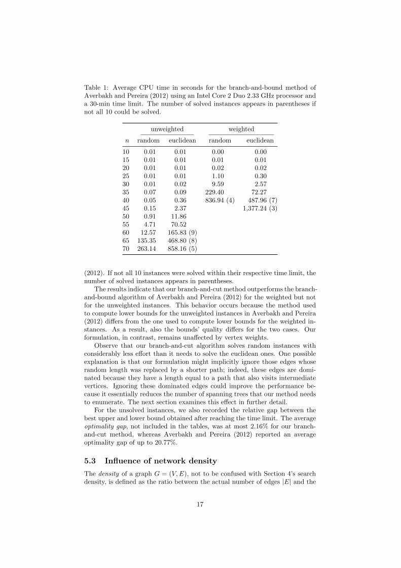
Table 1: Average CPU time in seconds for the branch-and-bound method ofAverbakh and Pereira (2012) using an Intel Core 2 Duo 2.33 GHz processor anda 30-min time limit. The number of solved instances appears in parentheses ifnot all 10 could be solved.

unweighted weighted

n random euclidean random euclidean

10 0.01 0.01 0.00 0.0015 0.01 0.01 0.01 0.0120 0.01 0.01 0.02 0.0225 0.01 0.01 1.10 0.3030 0.01 0.02 9.59 2.5735 0.07 0.09 229.40 72.2740 0.05 0.36 836.94 (4) 487.96 (7)45 0.15 2.37 1,377.24 (3)50 0.91 11.8655 4.71 70.5260 12.57 165.83 (9)65 135.35 468.80 (8)70 263.14 858.16 (5)

(2012). If not all 10 instances were solved within their respective time limit, thenumber of solved instances appears in parentheses.

The results indicate that our branch-and-cut method outperforms the branch-and-bound algorithm of Averbakh and Pereira (2012) for the weighted but notfor the unweighted instances. This behavior occurs because the method usedto compute lower bounds for the unweighted instances in Averbakh and Pereira(2012) differs from the one used to compute lower bounds for the weighted in-stances. As a result, also the bounds’ quality differs for the two cases. Ourformulation, in contrast, remains unaffected by vertex weights.

Observe that our branch-and-cut algorithm solves random instances withconsiderably less effort than it needs to solve the euclidean ones. One possibleexplanation is that our formulation might implicitly ignore those edges whoserandom length was replaced by a shorter path; indeed, these edges are domi-nated because they have a length equal to a path that also visits intermediatevertices. Ignoring these dominated edges could improve the performance be-cause it essentially reduces the number of spanning trees that our method needsto enumerate. The next section examines this effect in further detail.

For the unsolved instances, we also recorded the relative gap between thebest upper and lower bound obtained after reaching the time limit. The averageoptimality gap, not included in the tables, was at most 2.16% for our branch-and-cut method, whereas Averbakh and Pereira (2012) reported an averageoptimality gap of up to 20.77%.

5.3 Influence of network density

The density of a graph G = (V,E), not to be confused with Section 4’s searchdensity, is defined as the ratio between the actual number of edges |E| and the

17

Table 2: Average CPU time in seconds for our branch-and-cut algorithm usingan Intel Core i7-4790 3.60 GHz processor and a 20-min time limit. The numberof solved instances appears in parentheses if not all 10 could be solved.

unweighted weighted

n random euclidean random euclidean

10 0.15 0.15 0.15 0.1615 0.24 0.32 0.22 0.2920 0.98 1.09 0.67 1.0925 1.67 3.31 2.60 1.9430 2.34 7.76 2.76 22.1535 7.86 27.83 6.91 57.2440 10.05 60.82 13.54 110.6745 12.54 157.80 18.44 144.0450 71.44 192.16 (9) 48.60 (9) 161.69 (8)55 41.69 436.99 (7) 70.98 168.96 (6)60 98.79 577.51 (4) 112.21 (9) 683.07 (3)65 77.60 601.35 (3) 195.91 486.17 (4)70 166.78 (9) 162.57

maximum possible number of edges |V |(|V |−1)/2. To examine how the networkdensity influences the computational performance, a new set of test instanceswas generated in which we control for the network density. In particular, for allconsidered graph sizes and densities, ten instances were randomly generated asfollows. An integer weight av between 0 and 1000 was drawn randomly for eachvertex v ∈ V \ r, after which we set the probability pv = av/

∑w∈V \r aw.

To generate edges, first a spanning tree was constructed by randomly select-ing a sequence of edges and including the next edge whenever it connects twopreviously unconnected vertices. Secondly, edges were randomly added untilthe desired density was obtained. Edge lengths were generated by assigning anarbitrary point in the natural cube between 0 and 100 to each vertex and thentaking the rectilinear (or Manhattan) distance between those vertices that areconnected by an edge.

Table 3 shows that the network density strongly affects the CPU times. Forgraphs with n = 40 vertices and a density of 100%, for example, the averageCPU time exceeds the one for a density of 20% with almost factor ten. To a lesserextent, the average optimality gap for unsolved instances also seems to increasein the network density. As mentioned above, one possible reason why solvingdense graphs requires more effort is that our method needs to enumerate morespanning trees for these graphs. Indeed, the binary x-variables in our mixedinteger program essentially select a spanning tree, and the more such trees thegraph contains, the more branching needs to be done by the branch-and-cutalgorithm.

18

Table 3: Influence of network density on average CPU time (in seconds), numberof solved instances (# out of 10), and average optimality gap (in %) using a20-min time limit.

density = 20% density = 60% density = 100%

n CPU # gap CPU # gap CPU # gap

10 0.08 10 0.00 0.11 10 0.00 0.12 10 0.0020 0.27 10 0.00 0.52 10 0.00 0.79 10 0.0030 1.20 10 0.00 2.24 10 0.00 4.74 10 0.0040 2.20 10 0.00 8.19 10 0.00 20.19 10 0.0050 6.82 10 0.00 83.46 10 0.00 95.13 8 0.9560 59.34 9 0.32 141.96 9 0.79 291.45 7 0.5170 108.15 10 0.00 536.39 6 0.64 305.09 3 1.2980 194.68 10 0.00 478.04 5 0.91 720.39 2 0.9990 321.08 10 0.00 1,011.24 2 0.75

100 454.05 6 0.79110 676.50 4 0.38120 802.89 2 0.85

5.4 Quality of formulation, valid inequalities, and heuris-tics

Solving the linear programming (LP) relaxation obtained by relaxing the inte-grality constraints in our mixed integer program provides a lower bound on theminimal search cost. The greedy algorithm, on the other hand, yields an upperbound as it returns a feasible starting solution. The goal of adding the validinequalities (Section 3.3) and local search (Section 4.3), finally, is to tightenthese bounds. To assess the quality of our formulation, valid inequalities, andheuristics, we examine how close these bounds are to the minimal search cost.Figure 4 plots the average ratio (averaged over the 10 solved instances persetting) between the bounds and optimum as a function of network size anddensity.

With a lower bound always exceeding 97% of the minimal search cost, the LPrelaxation together with both cuts (C1) and (C2) provides a reasonable lowerbound. Although cuts (C2) do considerably increase the lower bound comparedto the formulation without valid inequalities, cuts (C1) clearly have the mostinfluence: the LP relaxation with only cuts (C1) achieves a lower bound onlymarginally weaker than the one with all cuts included.

Figure 4 also indicates that our heuristics provide high-quality solutions,especially when including the local search algorithm. On average, the greedysolution exceeds the optimal search cost with at most 4%, which drops to only0.27% after performing the local search. Moreover, out of all 379 instancessolved to optimality in our computational experiment, the local search couldfind the optimum for 305 instances and exceeded the minimal search cost withat most 2.15% for the other cases. With respect to computation times, thegreedy heuristic always required less than 0.3 seconds and the local search pro-cedure needed at most 100 seconds. We conclude that, empirically, the greedyalgorithm produces solutions much closer to optimality than the factor eight

19

Figure 4: Average ratio between bounds and the optimum. The bounds providedby the LP relaxation without cuts and with only cuts (C2) deteriorate as networksize and density increase, whereas the other bounds remain reasonably close tothe optimum.

(a) Ratio as a function of network size n for a given 60% network density.

10 30 50

0.78

0.84

0.97

1

1.04 greedy

local search

all cuts

cuts (C1)

cuts (C2)

no cuts

n

bound relative to optimum

(b) Ratio as a function of network density for a given network size n = 40.

20% 60% 100%

0.74

0.84

0.97

1

1.04 greedy

local search

all cuts

cuts (C1)

cuts (C2)

no cuts

density

bound relative to optimum

20

worst-case guarantee.Finally, observe that the lower bound provided by the LP relaxation without

cuts and with only cuts (C2) weakens as network size and density increase. Theother bounds, in contrast, seem to be more stable. This inverse relation betweennetwork density and the quality of the formulation without cuts constitutesanother reason why instances with a higher density require more effort: tomake up for the weaker lower bound, cuts need to be generated. Not onlydoes separating these cuts take time, but, more importantly, adding them alsoincreases the time needed to solve each LP relaxation because the model growsin size.

6 Discussion

We have studied exact and approximation algorithms for the expanding searchproblem, which has received increasing attention in the literature since its in-troduction by Alpern and Lidbetter (2013). Our novel branch-and-cut methodcan solve instances that were unsolved by existing algorithms and the greedyalgorithm described in this paper is the first constant-factor approximation al-gorithm established for the problem.

The formulation at the base of our branch-and-cut procedure builds uponresults from the single-machine scheduling literature and uncouples the selec-tion of a tree from the sequencing on that tree. We believe this could be afruitful approach for dealing with other scheduling problems as well. In partic-ular, our formulation seems generalizable to the problem of scheduling with ORprecedence constraints (Gillies and Liu, 1995).

Our results also contribute to the literature on search games. More specifi-cally, consider the expanding search game where the target acts as an adversarythat hides in one of the graph’s vertices in order to maximize the expected searchtime. Together with the work of Hellerstein et al. (2019), our branch-and-cutprocedure yields a method to compute the game’s value exactly, whereas ourgreedy approach allows to approximate this value within factor eight. Note thatthese results are incomparable with the approximations of Alpern and Lidbetter(2019) because, in that article, the target can hide at any point of an edge inthe network instead of being restricted to hide at vertices only.

The tree-based local search procedure introduced in Section 4.3 showedpromising results in computational experiments. We also established that itfinds a global optimum in case the underlying graph is a cycle, whereas othernatural approaches for local neighborhoods fail on these instances. Determiningthe actual worst-case guarantee of the local search is an interesting problem forfuture research.

Finally, in line with the work of Tan et al. (2019), it would be interesting togeneralize the expanding search model to multiple searchers. In fact, by takingthe search sequence returned by our greedy algorithm as a so-called ‘list sched-ule’, the techniques of Chekuri et al. (2001) and Tan et al. (2018, 2019) seemto provide a promising starting point to obtain constant-factor approximationalgorithms for the setting with multiple searchers.

21

Acknowledgments

Ben Hermans is funded by a PhD Fellowship of the Research Foundation –Flanders (Fonds Wetenschappelijk Onderzoek). We thank I. Averbakh and J.Pereira for kindly sharing their instances.

References

Afrati, F., Cosmadakis, S., Papadimitriou, C. H., Papageorgiou, G. and Pa-pakostantinou, N. (1986), ‘The complexity of the travelling repairman prob-lem’, RAIRO-Theoretical Informatics and Applications 20(1), 79–87.

Alpern, S., Fokkink, R., Gasieniec, L., Lindelauf, R. and Subrahmanian, V.(2013), Search Theory, Springer.

Alpern, S. and Gal, S. (2003), The Theory of Search Games and Rendezvous,Kluwer International Series in Operations Research and Management Sciences(Kluwer, Boston).

Alpern, S. and Lidbetter, T. (2013), ‘Mining coal or finding terrorists: Theexpanding search paradigm’, Operations Research 61(2), 265–279.

Alpern, S. and Lidbetter, T. (2019), ‘Approximate solutions for expand-ing search games on general networks’, Annals of Operations Research275(2), 259–279.

Angelopoulos, S., Durr, C. and Lidbetter, T. (2019), ‘The expanding searchratio of a graph’, Discrete Applied Mathematics 260, 51–65.

Archer, A., Levin, A. and Williamson, D. P. (2008), ‘A faster, better approxi-mation algorithm for the minimum latency problem’, SIAM Journal on Com-puting 37(5), 1472–1498.

Ausiello, G., Leonardi, S. and Marchetti-Spaccamela, A. (2000), On salesmen,repairmen, spiders, and other traveling agents, in ‘Italian Conference on Al-gorithms and Complexity’, Springer, pp. 1–16.

Averbakh, I. (2012), ‘Emergency path restoration problems’, Discrete Optimiza-tion 9(1), 58 – 64.

Averbakh, I. and Pereira, J. (2012), ‘The flowtime network construction prob-lem’, IIE Transactions 44(8), 681–694.

Chekuri, C., Motwani, R., Natarajan, B. and Stein, C. (2001), ‘Approxima-tion techniques for average completion time scheduling’, SIAM Journal onComputing 31(1), 146–166.

Correa, J. R. and Schulz, A. S. (2005), ‘Single-machine scheduling with prece-dence constraints’, Mathematics of Operations Research 30(4), 1005–1021.

Feige, U., Lovasz, L. and Tetali, P. (2004), ‘Approximating min sum set cover’,Algorithmica 40(4), 219–234.

22

Fokkink, R., Lidbetter, T. and Vegh, L. A. (2019), ‘On submodular search andmachine scheduling’, Mathematics of Operations Research pp. 1–19. ePubahead of print August 1, https://doi.org/10.1287/moor.2018.0978.

Ford, L. R. and Fulkerson, D. R. (1956), ‘Maximal flow through a network’,Canadian Journal of Mathematics 8, 399–404.

Gillies, D. W. and Liu, J. W.-S. (1995), ‘Scheduling tasks with AND/OR prece-dence constraints’, SIAM Journal on Computing 24(4), 797–810.

Goemans, M. X. and Williamson, D. P. (1995), ‘A general approximationtechnique for constrained forest problems’, SIAM Journal on Computing24(2), 296–317.

Goldberg, A. V. and Tarjan, R. E. (1988), ‘A new approach to the maximum-flow problem’, Journal of the ACM 35(4), 921–940.

Hegde, C., Indyk, P. and Schmidt, L. (2015), A nearly-linear time framework forgraph-structured sparsity, in ‘International Conference on Machine Learning’,pp. 928–937.

Hellerstein, L., Lidbetter, T. and Pirutinsky, D. (2019), ‘Solving zero-sum gamesusing best-response oracles with applications to search games’, OperationsResearch 67(3), 731–743.

Kao, M.-J., Katz, B., Krug, M., Lee, D., Rutter, I. and Wagner, D. (2013),‘The density maximization problem in graphs’, Journal of Combinatorial Op-timization 26(4), 723–754.

Koopman, B. O. (1956a), ‘The theory of search I: Kinematic bases’, Operationsresearch 4(3), 324–346.

Koopman, B. O. (1956b), ‘The theory of search II: Target detection’, Operationsresearch 4(5), 503–531.

Koopman, B. O. (1957), ‘The theory of search III: The optimum distribution ofsearching effort’, Operations Research 5(5), 613–626.

Koutsoupias, E., Papadimitriou, C. and Yannakakis, M. (1996), Searching afixed graph, in F. Meyer and B. Monien, eds, ‘Automata, Languages andProgramming’, Springer Berlin Heidelberg, Berlin, Heidelberg, pp. 280–289.

Lau, H. C., Ngo, T. H. and Nguyen, B. N. (2006), ‘Finding a length-constrainedmaximum-sum or maximum-density subtree and its application to logistics’,Discrete Optimization 3(4), 385–391.

Li, S. and Huang, S. (2018), ‘Multiple searchers searching for a randomly dis-tributed immobile target on a unit network’, Networks 71(1), 60–80.

Magnanti, T. L. and Wolsey, L. A. (1995), Optimal trees, in M. O. Ball,T. L. Magnanti, C. L. Monma and G. L. Nemhauser, eds, ‘Network Mod-els’, Vol. 7 of Handbooks in Operations Research and Management Science,Elsevier, pp. 503–615.

23

Monma, C. L. and Sidney, J. B. (1979), ‘Sequencing with series-parallel prece-dence constraints’, Mathematics of Operations Research 4(3), 215–224.

Potts, C. N. (1980), ‘An algorithm for the single machine sequencing problemwith precedence constraints’, Mathematical Programming Studies 13, 78–87.

Queyranne, M. and Wang, Y. (1991), ‘Single-machine scheduling polyhedra withprecedence constraints’, Mathematics of Operations Research 16(1), 1–20.

Sidney, J. B. (1975), ‘Decomposition algorithms for single-machine sequencingwith precedence relations and deferral costs’, Operations Research 23(2), 283–298.

Sitters, R. (2002), The minimum latency problem is NP-hard for weighted trees,in ‘International Conference on Integer Programming and Combinatorial Op-timization’, Springer, pp. 230–239.

Smith, W. E. (1956), ‘Various optimizers for single-stage production’, NavalResearch Logistics Quarterly 3(1-2), 59–66.

Stone, L. D. (2007), Theory of Optimal Search, 2nd edition, INFORMS.

Stone, L. D., Royset, J. O. and Washburn, A. R. (2016), Optimal Search forMoving Targets, Springer.

Tan, Y., Qiu, F., Das, A. K., Kirschen, D. S., Arabshahi, P. and Wang, J.(2018), ‘Scheduling post-disaster repairs in electricity distribution networks’,ArXiv e-prints arXiv:1702.08382 pp. 1–23. https://arxiv.org/pdf/1702.

08382.pdf.

Tan, Y., Qiu, F., Das, A. K., Kirschen, D. S., Arabshahi, P. and Wang, J.(2019), ‘Scheduling post-disaster repairs in electricity distribution networks’,IEEE Transactions on Power Systems 34(4), 2611–2621.

Trummel, K. and Weisinger, J. (1986), ‘The complexity of the optimal searcherpath problem’, Operations Research 34(2), 324–327.

24