exact fit to the swaption volatility matrix using semide...

Exact Fit to the Swaption Volatility MatrixUsing Semidefinite Programming∗

Alan Brace†and Robert S. Womersley‡

Working paper presented at

ICBI Global Derivatives Conference

Paris, April 2000

Abstract

This paper addresses the problem of parameterizing jointly to all swaptions inthe framework of the lognormal Libor market model (LLMM). First we refine someprevious work showing that swaprates are nearly lognormal with a deterministicvolatility. Then we formulate the fitting problem in terms of covariance matricesrather than the usual two variable volatility function. Semidefinite programming,in which the variables are positive semidefinite matrices (covariance matrices),minimizes a linear function of the variables subject to linear constraints on thevariables. Exact fits to the swaption volatility matrix are imposed through linearconstraints on covariance matrices. Various objectives can be used to get close toa historical covariance matrix. The method is illustrated by pricing fixed maturityBermudan options.

Keywords: lognormal Libor market model, swaption volatility matrix, covariancematrix, semidefinite programming, Bermudan option.

∗The authors would like to thank National Australia Bank for its support and Paul O’Brien for hishelp and comments

†National Australia Bank <[email protected]>‡School of Mathematics, University of New South Wales <[email protected]>,

http://www.maths.unsw.edu.au/~rsw

1

Fitting Swaption Volatilities using Semidefinite Programming 2

Contents

1 Introduction 2

2 Swaprate Volatilities in the LLMM 42.1 Some low variance and other martingales . . . . . . . . . . . . . . . . . . 62.2 Swaprate Analysis . . . . . . . . . . . . . . . . . . . . . . . . . . . . . . 82.3 Swaprate Volatility Analysis . . . . . . . . . . . . . . . . . . . . . . . . . 102.4 Swaption values . . . . . . . . . . . . . . . . . . . . . . . . . . . . . . . . 11

3 Semidefinite programming 123.1 Semidefinite/Covariance matrices . . . . . . . . . . . . . . . . . . . . . . 123.2 Objective functions . . . . . . . . . . . . . . . . . . . . . . . . . . . . . . 14

4 Volatility Structure 164.1 Cap and swaption volatilities . . . . . . . . . . . . . . . . . . . . . . . . 164.2 Choice of volatility function . . . . . . . . . . . . . . . . . . . . . . . . . 164.3 Simplification . . . . . . . . . . . . . . . . . . . . . . . . . . . . . . . . . 184.4 Implied Correlation . . . . . . . . . . . . . . . . . . . . . . . . . . . . . . 19

5 Numerical Results 205.1 Volatility data . . . . . . . . . . . . . . . . . . . . . . . . . . . . . . . . . 205.2 Covariance approximation . . . . . . . . . . . . . . . . . . . . . . . . . . 225.3 Bermudan prices . . . . . . . . . . . . . . . . . . . . . . . . . . . . . . . 24

1 Introduction

Most professionals now regard the so called market models (see [17] for a review) asthe best starting point for pricing caps, swaptions and associated exotics. These modelsare arbitrage free, lognormal, return Black cap or swaption formulae, have two variable(time/maturity) volatility functions, and input today’s yield curve as an initial value.The lognormal Libor market model (LLMM) parameterizes accurately to the cap stripand returns caplet prices that agree with Black values, while the lognormal swapratemodel (LSRM) parameterizes accurately to some subsets of the swaption volatility ma-trix (like the reverse diagonal), and returns some Black swaption values. Outstandingproblems that have been considered but not settled are: parameterizing jointly to allswaptions; including caps in the swaption parameterization; and fitting cap and swap-tion volatility skews [3]. We address the first.

It is important to realize that if all swaptions are to be fitted without compromisingthe model, then it is prices rather than volatilities that must be fitted, which leads toa highly non-linear optimization problem (the first author has discouraging memoriesof genetic algorithm routines that took hours and never gave similar answers twice).Clearly, fitting volatilities is simpler, because it cuts out the complexities of the Black


formula. But then, because only a subset of swaption volatilities can be returned withoutcompromising the model, approximation becomes the necessary price of tractability. Wechoose to make such approximations within the LLMM because it is relatively easy(analytically and computationally), but in principle other market models could be used.

Thus we aim to exactly fit in the LLMM a matrix of approximate swaption volatilities.Our approach involves three main steps:

1. In Section 2 we refine some of the arguments in [6] and [7] which showed thatswaprates in the LLMM are virtually lognormal with nearly deterministic volatility.The necessary approximations work because certain low variance martingales areset equal to their start values. We checked these approximations by confirming thatour parameterized models returned, via simulation, those prices that are input tothe parameterization.

2. Secondly (see Sections 2 and 4) we decided to work with covariance matrices1 ratherthan the volatility functions from which they are formed, as that removed anotherlayer of complexity. Except for the case of piecewise constant volatility (which iswhat we use here), reversing this step to obtain continuous volatility functions isnot trivial.

3. Thirdly (see Sections 3 and 4) we realized that given the right volatility structureand optimization objective, the problem was solvable using the recently developedtechniques of semidefinite programming (analogous to linear programming exceptthe variables are semidefinite matrices rather than non-negative vectors).

Considerable experimentation led us to volatility functions of the form (with standardnotation)

γ(t, T ) = φ(t)ξ(T − t),

in which φ(·) is piecewise constant. These volatility functions can be thought of as being“homogeneous in layers” determined by time t. Swaption volatilities then turn out to besimple linear combinations of covariance matrices, leading to linear equality constraintsin the semidefinite framework. Moreover, because ξ(·) is homogeneous, instantaneouscorrelation can be sensibly defined, so our objective function can be made to target his-toric covariance in some way. The resulting parameterizations fit all swaption volatilitieswith a correlation structure not too different from the historic one. That correlationstructure can be thought of as implied correlation.

Of course we parameterized to European swaptions and got back, via simulation,the values input to the parameterization. In addition we decided to test our techniqueon fixed maturity Bermudans because they tend to be parameterized on a deal-by-dealbasis. Specifically, we were interested in whether, with just one parameterization andover a range of data, our method could return similar prices to the standard models for

1Our thanks to Marek Musiela for this suggestion.


Bermudans using two significantly different reverse diagonals. The results (see Section 5)surprised us: our Bermudan prices were either roughly equal to, or less than, prices fromthe standard single factor models.

We are uncertain of what to make of our finding, but take comfort from the factthat Bermudans have been priced with single factor models for a long time, with only acouple (as far as we know) of rumoured instances of significant writeoffs. The point isthat, because banks tend to be overall buyers of Bermudans, such writeoffs would likelyarise from models that overprice rather than underprice.

2 Swaprate Volatilities in the LLMM

The background to this section is [6], in which Brace et al showed LLMM swaprates werestatistically lognormal and derived approximate formulae for their volatilities, and [7]in which Barton et al investigated hedging implications. We show the relative accuracyof these approximations stems from certain low variance martingales being set equal totheir start values, and in Theorem 2.4 slightly tighten their approximation ([6], page 9equation (23)) for swaprate volatility in the LLMM.

For arbitrary time T let WT and ET denote Brownian motion and expectation re-spectively under the forward measure PT . In particular let W0 and E0 denote Brownianmotion and expectation under the arbitrage free measure. Also let P (t, T ) denote thetime t-price of a zero coupon bond maturing at an arbitrary time T , and set Tj = T + jδfor j = 1, 2, . . . , n. Then in the LLMM simple forwards

K(t, T ) =1

δ

{P (t, T )

P (t, T1)− 1

}over arbitrary δ-intervals [T, T + δ] are lognormal with deterministic volatility γ(t, T )and

dK(t, T ) = K(t, T )γ(t, T )dWT1(t)

under forward measures PT1 at the ends of their intervals. Moreover, see [8], the corre-sponding stochastic HJM volatility σ(t, T ) satisfies∫ T1

T

σ(t, u)du =δK(t, T )

1 + δK(t, T )γ(t, T ) = µ(t, T )γ(t, T ), (2.1)

where

µ(t, T ) =δK(t, T )

1 + δK(t, T ). (2.2)

In addition it is easy to show that forward contracts

FT (t, Tj) =P (t, Tj)

P (t, T ),


expiring at T and maturing at Tj, satisfy stochastic differential equations SDEs like

dFT (t, Tj) = −FT (t, Tj)

∫ Tj

T

σ(t, u)dudWT (t), (2.3)

d [FT (t, Tj)K(t, Tj−1)]

FT (t, Tj)K(t, Tj−1)=

{γ(t, Tj−1)−

∫ Tj

T

σ(t, u)du

}dWT (t).

Let K(t, T, r) be the forward over the interval [T, T + δr] defined by

FT (t, T + δr) =P (t, T + δr)

P (t, T )=

1

1 + rδK(t, T, r).

The time t value of an r-period payer swap in which the floating forward K(t, Tj−r, r)over the interval [Tj−r, Tj ] is swapped in arrears against fixed κ at n/r intervals of rδ,can be expressed as the weighted sum of the simple forwards K(t, Tj) like

Pswap(t, T, r, n) = E0

{n∑

j=1

roz(j, r)β(t)

β(Tj)δ [K(t, Tj−r, r)− κ]

∣∣∣∣∣Ft

},

= δn∑

j=1

P (t, Tj) [K(t, Tj−1) − roz(j, r)κ] ,

where β(·) is the HJM bank account and roz(·) is the r or zero function

roz(j, r) =

{r if j mod r = 0,0 otherwise.

Introducing the corresponding r-period swap rate

ω(t, T, r, n) =

∑nj=1 FT (t, Tj)K(t, Tj−1)∑n

j=1 roz(j, r)FT (t, Tj), (2.4)

this payer swap can be rewritten

Pswap(t, T, r, n) = δn∑

j=1

roz(j, r)P (t, Tj)[ω(t, T, r, n)− κ].

A payer swaption exchanges in arrears at n/r consecutive intervals of rδ the time Tswaprate ω(T, T, r, n) against the strike κ when ω(t, T, r, n) ≥ κ, and so has value

Pswpn(t, T, r, n) = E0

{n∑

j=1

roz(j, r)β(t)

β(Tj)δ[ω(t, T, r, n)− κ]+

∣∣∣∣∣Ft

}, (2.5)

= δP (t, T )ET

{n∑

j=1

roz(j, r)FT (T, Tj)[ω(t, T, r, n)− κ]+

∣∣∣∣∣Ft

}.

We will tackle this expectation by showing that under a new measure P(r)T equivalent to

PT , the r-period swaprate ω(t, T, r, n) is close to lognormal.


2.1 Some low variance and other martingales

The first set of (low variance) martingales are the µ(t, T ) defined in (2.1). From (2.3),it is easy to show

µ(t, T ) = 1− 1

1 + δK(t, T )= 1− FT (t, T1) ∈ [0, 1] ,

dµ(t, T ) = [1− µ(t, T )]µ(t, T )γ(t, T )dWT (t)

=δK(t, T )

[1 + δK(t, T )]2γ(t, T )dWT (t),

demonstrating that µ(t, T ) is a PT -martingale. The [1− µ(t, T )] term in the SDE pre-vents us viewing µ(t, T ) as an exponential martingale with a stochastic volatility wemight find to be small. But in absolute terms, not only is µ(t, T ) bounded in [0, 1], butits absolute volatility is a couple of orders of magnitude (δK(t, T ) ∼= 1%− 2%) less thanthe volatilities of the forwards. For this reason, we will approximate µ(t, T ) with its zerovalue

µ(t, T ) ∼= µ(0, T ) =δK(0, T )

1 + δK(0, T )(2.6)

for all maturities T .With the aid of the SDEs (2.3), the following result (which is an easy exercise) helps

us analyze the stochastic behaviour of the swaprate (2.4).

Theorem 2.1 Under some measure P, let Y (t) be an Ito process with SDE

dY (t)

Y (t)= η(t)dt+ ξ(t)dW (t),

and let Xj, j = 1, . . . , n be exponential martingales with SDEs

dXj(t)

Xj(t)= σj(t)dW (t),

where the ηt), ξ(t) and σj(t) may be stochastic. Then the variable

Z(t) =Y (t)∑n

j=1 roz(j, r)Xj(t),

(1 ≤ j ≤ n, nmod r = 0) satisfies the SDE

dZ(t)

Z(t)= η(t)dt+

[ξ(t)−

∑nj=1 roz(j, r)Xj(t)σj(t)∑n

j=1 roz(j, r)Xj(t)

]dW (r)(t);

dW (r)(t) = dW (t)−∑n

j=1 roz(j, r)Xj(t)σj(t)∑nj=1 roz(j, r)Xj(t)

dt.


Remark 2.2 If η(t) = 0 so that Y (t) is a P-martingale, then clearly Z(t) will be an

exponential martingale under the measure P(r) induced by W (r)(t). In other words, given

some exponential martingales under a measure P, one martingale divided by the sum ofothers, will itself be an exponential martingale, but under another measure P

(r) equivalentto P.

The second set of (low variance) martingales are the weights uj(t) of the K(t, Tj−1)in the swaprate formula (2.4), namely

uj(t) =FT (t, Tj)∑n

j=1 roz(j, r)FT (t, Tj)j = 1, . . . , n. (2.7)

If Xj(t) = FT (t, Tj) and Y (t) = FT (t, Tj) in Theorem 2.1, then using (2.3)

duj(t)

uj(t)=

[−∫ Tj

T

σ(t, u)du+

n∑j=1

roz(j, r)uj(t)

∫ Tj

T

σ(t, u)du

]dW

(r)T (t), (2.8)

dW(r)T (t) = dWT (t) +

n∑j=1

roz(j, r)uj(t)

∫ Tj

T

σ(t, u)du dt.

The weights uj(t) will all be martingales under the measure P(r)T induced by W

(r)T (t), and

because the plus and minus terms in (2.8) are roughly equal, their volatilities will tendto be small, making their initial values uj(0) good approximations to subsequent values.

The third set of (not low variance) martingales are the actual terms in the swaprate(2.4) as a whole, namely

vj(t) =FT (t, Tj)K(t, Tj−1)∑nj=1 roz(j, r)FT (t, Tj)

j = 1, . . . , n. (2.9)

If Xj(t) = FT (t, Tj) and Y (t) = FT (t, Tj)K(t, Tj−1) in Theorem 2.1, then using (2.3)

dvj(t)

vj(t)=

[γ(t, Tj−1)−

∫ Tj

T

σ(t, u)du+

n∑j=1

roz(j, r)uj(t)

∫ Tj

T

σ(t, u)du

]dW

(r)T (t); (2.10)


n∑j=1

roz(j, r)uj(t)

∫ Tj

T

σ(t, u)du dt.

Hence the vj(t) will also be martingales under the measure P(r)T induced by W

(r)T (t). Note,

however, that the volatility of vj(t) will be approximately γ(t, Tj−1), which is not small.Because it is convenient to cover them here, we also identify two other types of

martingales which will appear later.


A fourth set of (low variance) martingales are the weights in the expression (2.19)below for swaprate volatility, namely

wj(t) =FT (t, Tj)K(t, Tj−1)∑nj=1 FT (t, Tj)K(t, Tj−1)

j = 1, . . . , n. (2.11)

If Xj(t) = FT (t, Tj)K(t, Tj−1) and Y (t) = FT (t, Tj)K(t, Tj−1) in Theorem 2.1, then from(2.3)

dwj(t)

wj(t)=

[γ(t, Tj−1)−

∫ Tj

T

σ(t, u)du

−n∑

j=1

wj(t)

{γ(t, Tj−1) −

∫ Tj

T

σ(t, u)du

}]dW ∗

T (t); (2.12)

dW ∗T (t) = dWT (t) −

n∑j=1

wj(t)

{γ(t, Tj−1)−

∫ Tj

T

σ(t, u)du

}dt.

The weights wj(t) will all be martingales under the measure P∗T induced by W ∗

T (t) and,again because the plus and minus terms in (2.12) are roughly equal, their volatilitieswill tend to be small, again making their initial values wj(0) good approximations tosubsequent values.

A fifth and final type of martingale helps change measure between PT and P(r)T , see

Theorem 2.3 below. If Xj(t) = FT (t, Tj) and Y (t) = 1 in Theorem 2.1, then using (2.3)

d

(1∑n

j=1 roz(j, r)FT (t, Tj)

)(

1∑nj=1 roz(j, r)FT (t, Tj)

) =

[n∑

j=1

roz(j, r)uj(t)

∫ Tj

T

σ(t, u)du

]dW

(r)T (t). (2.13)

showing the reciprocal of∑n

j=1 roz(j, r)FT (t, Tj) is yet another martingale under the

measure P(r)T induced by W

(r)T (t).

2.2 Swaprate Analysis

In the LLMM, define the swaprate measure P(r)T , to be the measure equivalent to PT

induced by the Brownian motion W(r)T (t) appearing in formulae (2.8) and (2.10) above,


n∑j=1

roz(j, r)uj(t)

∫ Tj

T

σ(t, u)du dt. (2.14)

Note that the W(r)T (t) can be expressed as the uj(t)-weighted sum of the forward Brow-

nian motions WTj(t) under the forward measures PTj

dW(r)T (t) =

n∑j=1

roz(j, r)uj(t)dWTj(t),


which means, intuitively, that the swaprate Brownian motion W(r)T (t) is not too different

from any of the forward Brownian motions WTj(t).

Using (2.4) and (2.10), after some rearrangement, an SDE for the forward swaprateω(t, T, r, n), is

dω(t, T, r, n)

ω(t, T, r, n)=

n∑j=1

{wj(t)γ(t, Tj−1) +

[roz(j, r)uj(t)− wj(t)]

∫ Tj

T

σ(t, u)du

}dW

(r)T (t) (2.15)

= σ(t, T, r, n)dW(r)T (t),

showing that within the LLMM each swaprate ω(t, T, r, n), of whatever length nδ, ma-

turity T or roll r, will be a martingale under the corresponding swaprate measure P(r)T .

We intend to show that the volatility σ(t, T, r, n) is nearly deterministic.

To change measures between PT and P(r)T use

Theorem 2.3 For 0 ≤ t ≤ T ∗ ≤ T < Tj

ET {f(T ∗)| Ft} =

n∑j=1

roz(j, r)FT (t, Tj)E(r)T

{f(T ∗)∑n

j=1 roz(j, r)FT (T ∗, Tj)

∣∣∣∣∣Ft

},

E(r)T {g(T ∗)| Ft} =

1∑nj=1 roz(j, r)FT (t, Tj)

ET

{g(T ∗)

n∑j=1

roz(j, r)FT (T ∗, Tj)

∣∣∣∣∣Ft

}.

Proof: From (2.14)

dWT (t) = dW(r)T (t)−

n∑j=1

roz(j, r)uj(t)

∫ Tj

T

σ(t, u)du dt,

and so from Girsanov and (2.13), change of measure will be given by

ET {f(T ∗)| Ft} = E(r)T

{E{∫ T

t

n∑j=1

roz(j, r)uj(s)

∫ Tj

T

σ(s, u)dudWT (s)

}f(T ∗)

∣∣∣∣∣Ft

}

= E(r)T

{ ∑nj=1 roz(j, r)FT (t, Tj)∑nj=1 roz(j, r)FT (T, Tj)

f(T ∗)

∣∣∣∣∣Ft

}

=n∑

j=1

roz(j, r)FT (t, Tj)E(r)T

{f(T ∗)∑n

j=1 roz(j, r)FT (T ∗, Tj)

∣∣∣∣∣Ft

},

because1∑n

j=1 roz(j, r)FT (T ∗, Tj)is a P

(r)T -martingale.


A change of measure from PT to P(r)T transforms the swaption formula (2.5) to

Pswpn(t, T, r, n) = δ

[n∑

j=1

roz(j, r)P (t, Tj)

]E

(r)T

{[ω(T, T, r, n)− κ]+

∣∣Ft

}(2.16)

which would lead to the Black swaption formula if ω(t, T, r, n) were lognormal under P(r)T .

2.3 Swaprate Volatility Analysis

In [6] it was demonstrated by simulation, that swaprates are statistically lognormal,indicating that the volatility term

σ(t, T, r, n) =n∑

j=1

{wj(t)γ(t, Tj−1) + [roz(j, r)uj(t)− wj(t)]

∫ Tj

T

σ(t, u)du

}, (2.17)

in (2.15) is close to deterministic. Moreover, if in (2.15) we assume

n∑j=1

[roz(j, r)uj(t)− wj(t)]

∫ Tj

T

σ(t, u)du ∼= 0, (2.18)

and approximate the wj(t) by their initial values wj(0), then we obtain equation (23) onpage 9 of [6], which produced swaption values accurate to within 1− 2%.

To get a more exact approximation include the terms (2.18). From (2.2)∫ Tj

T

σ(t, u)du =

j∑`=1

µ(t, T`−1)γ(t, T`−1),

where each µ(t, T`−1) is a low variance PT`-martingale. Substituting in (2.17), the in-

stantaneous swaprate volatility σ(t, T, r, n) therefore becomes

σ(t, T, r, n) =n∑

j=1

{wj(t)γ(t, Tj−1) +

[roz(j, r)uj(t) − wj(t)]

j∑`=1

µ(t, T`−1)γ(t, T`−1)

}, (2.19)

=n∑

j=1

γ(t, Tj−1)

{wj(t) + µ(t, Tj−1)

n∑`=j

[roz(`, r)u`(t) − w`(t)]

},

=

n∑j=1

Aj(t)γ(t, Tj−1)

where

Aj(t) = wj(t) + µ(t, Tj−1)

n∑`=j

[roz(`, r)u`(t) − w`(t)] , (2.20)


and wj(t), µ(t, Tj−1) and u`(t) are defined by (2.11), (2.2) and (2.7) above.As remarked above, the uj(t), wj(t) and µ(t, T`−1) are low variance.martingales under

their respective measures. So approximating them by their initial values is not unrea-sonable, and gives the following fundamental and important result:

Theorem 2.4 In the LLMM, swaprates are almost lognormal, with a volatility that canbe closely approximated by the deterministic vector volatility function

σ(t, T, r, n) =n∑

j=1

Ajγ(t, Tj−1), (2.21)

where, for j = 1, . . . , n,

Aj = wj(0) + µ(0, Tj−1)n∑

`=j

[roz(`, r)u`(0)− w`(0)] , (2.22)

wj(0) =FT (0, Tj)K(0, Tj−1)∑nj=1 FT (0, Tj)K(0, Tj−1)

,

µ(0, Tj−1) =δK(0, Tj−1)

1 + δK(0, Tj−1),

uj(0) =FT (0, Tj)∑n

j=1 roz(j, r)FT (0, Tj).

2.4 Swaption values

Using (2.16) with the approximation (2.21), the present (time t = 0) value of a payerswaption will be

Pswpn(0, T, r, n) ∼= δ

[n∑

j=1

roz(j, r)P (0, Tj)

]E

(r)T

{[ω(0, T, r, n)e(Z)− κ]+

}, (2.23)

where, under the swaprate measure P(r)T

Z ∼ N(0, β2T ),

e(Z) = exp

(Z − 1

2VarZ

),


and the Black volatility β(T, r, n) of the swaption and its swaption zeta ζ(T, r, n) aregiven by

ζ(T, r, n) = β(T, r, n)2 T (2.24)

=

∫ T

0

|σ(s, T, r, n)|2 ds

=

∫ T

0

n∑j=1

|Ajγ(s, Tj−1)|2 ds

=

n∑i=1

n∑j=1

AiAj

∫ T

0

γ∗(s, Ti−1)γ(s, Tj−1)ds,

=n∑

i=1

n∑j=1

AiAj∆i,j

in which

∆ = (∆i,j) =

(∫ T

0

γ∗(s, Ti−1)γ(s, Tj−1)

)is the swap quadratic variation matrix. A closed formula for the approximate presentvalue of the swaption is therefore

Pswpn(0, T, r, n) ∼= δ

n∑j=1

roz(j, r)P (0, Tj)B {T, r, n, κ, ω(0, T, r, n), β(T, r, n)} , (2.25)

where B(·) is the Black futures formula.

3 Semidefinite programming

Semidefinite programming (SDP) is a relatively recent extension of linear programmingin which the variables are positive semidefinite matrices, rather than vector of non-negative variables as in linear programming. General references on semidefinite pro-gramming include the review article by Vandenberghe and Boyd [23], the special issue ofMathematical Programming edited by Overton and Wolkowicz [20], and more recentlythe Handbook of Semidefinite Programming [25].

3.1 Semidefinite/Covariance matrices

Let Sn denote the space of real symmetric n× n matrices, that is

Sn = {X ∈ Rn×n : XT = X}.


The natural inner product on the vector space Sn is the Frobenius inner product

X • Y = trace(XTY ) =n∑

i=1

n∑j=1

XijYij, X, Y ∈ Sn,

which induces the Frobenius norm ‖X‖F defined by

‖X‖2F = X •X.

A matrix X ∈ Sn is positive semidefinite (written X � 0) if any one of the followingequivalent conditions hold:

1. For every vector w ∈ Rn, wTXw ≥ 0.

2. Every eigenvalue of X is nonnegative: λi(X) ≥ 0, i = 1, . . . , n.

3. The Cholesky factorization X = LLT , where L ∈ Rn is lower triangular, exists.

4. X has a square root Y ∈ Sn such that X = Y Y T .

5. X • Y ≥ 0 for every Y ∈ Sn, Y � 0.

Remark 3.1 These are precisely the class of matrices of interest to us because a matrixX ∈ Sn is a covariance matrix iff X is positive semidefinite (see [16] for example).

Semidefinite programming deals with optimization problems of the form

find X ∈ Sn

to minimize C •Xsubject to Ak •X = bk k = 1, . . . , m

X � 0,

(3.1)

where C ∈ Sn, Ak ∈ Sn for k = 1, . . . , m, and bk ∈ R for k = 1, . . . , m are given data.Here the objective function C •X and constraints Ak •X = bk are all linear functionsof the variables X. The set {X ∈ Sn : X � 0} is a convex cone, but is not polyhedral,unlike {x ∈ R

n : x ≥ 0} which is a polyhedral convex cone.The dual problem is

find y ∈ Rm

to maximize yT bsubject to C −∑m

k=1 ykAk � 0.(3.2)

Weak duality holds in that if X ∈ Sn is feasible for (3.1) and y ∈ Rm is feasible in (3.2),

then C • X ≥ yT b. If both the primal problem (3.1) and the dual problem (3.2) havestrictly feasible points (a stronger condition than is required in linear programming),then the primal and dual objective values are equal at a solution. The dual formulationis most commonly used in the control theory literature (see [5] for example).


Linear programming is just a special case of semidefinite programming in which thematrices are diagonalX = diag(x) and Ak = diag(ak) where x, ak ∈ R

n, so X•Ak = aTk x.

Several different semidefinite matrices X1, X2, . . . , Xp can be accumulated into one largerblock diagonal semidefinite matrix X = diag(X1, X2, . . . , Xp).

We will consider a standard problem which explicitly includes both symmetric posi-tive semidefinite matrix variables and vectors of non-negative variables:

find X ∈ Sn, x ∈ Rn

to minimize C •X + cTxsubject to Ak •X = bk k = 1, . . . , ms,

aTj x = βj j = 1, . . . , ml,X � 0, x ≥ 0.

(3.3)

Here X and Ak, k = 1, . . . , ms are symmetric block diagonal matrices, each with p blocksof size n1, . . . , np, where n =

∑pi=1 ni.

Karmarkar’s 1984 polynomial time algorithm for linear programming lead to an ex-plosion of work in interior point methods for linear programming (see [24] for example).Many of the extensions to more general convex programs were pioneered by Nesterovand Nemirovski [19]. Instead of following edges of the feasible region {x ∈ R

n : Ax =b, x ≥ 0} to a minimum vertex as in the simplex method for linear programming, inte-rior point methods use strictly positive iterates x > 0 and follow the “central path” to asolution. In linear programming the nonnegative orthant x ≥ 0 is a polyhedral convexcone, so the feasible region is the intersection of hyperplanes and a polyhedral convexcone. In semidefinite programming the variables are symmetric matrices X ∈ Sn, whichmust lie in the convex (but not polyhedral) cone X � 0 intersected with hyperplanesX • Ak = bk for k = 1, . . . , m. Because they move through the interior of the coneconstraint, interior point methods have been successfully generalized to provide efficientmethods for semidefinite programming (see [1, 22] for example).

3.2 Objective functions

Many different problems can be formulated as semidefinite problems (see [23]). In par-ticular semidefinite programming is closely related to eigenvalue optimization problems.If λ1, λ2, . . . , λn are the eigenvalues of X, then

I •X = trace(X) =

n∑i=1

λi,

(where I is the appropriately sized identity matrix). The expression I •X is one of thesimplest objective functions to minimize in semidefinite programming, and can be usedto “minimize” the size of X � 0.

The largest eigenvalue of a symmetric matrix can be minimized subject to the con-


straints Ak •X = bk, k = 1, . . . , m, by adding a further constraint, and solving

find X ∈ Sn, ζ ∈ R

to minimize ζsubject to ζI −X � 0,

Ak •X = bk, k = 1, . . . , ms.

(3.4)

This can be simply justified by noting that the eigenvalues of ζI − X are ζ − λi(X),so that ζI − X � 0 is equivalent to ζ ≥ λi(X) for i = 1, . . . , n. Problem (3.4) can beconverted into the form (3.3) by adding a surplus matrix S = ζI −X � 0.

The fit to the swaption volatility matrix is imposed through linear constraints of theform Ak • X = bk (see Section 4), while a variety of different objectives can be used.In particular we are interested in making the positive semidefinite covariance matrix“close” to a historical covariance matrix G. The difference X − G is in general notpositive semidefinite, so simple objective like trace(X − G) or the largest eigenvalue ofX −G will not work.

We cannot use the Frobenius norm, or its square, directly to force X close to a targetmatrix G ∈ Sn because ‖X − G‖2

F = (X −G) • (X −G) is not linear in X. However avariety of other matrix norms can be used. The 2−norm,

‖X −G‖2 = maxi=1,... ,n

|λi(X −G)|

can be minimized by adding two further constraints and solving

find X ∈ Sn, ζ ∈ R

to minimize ζsubject to ζI − (X −G) � 0,

ζI + (X −G) � 0,Ak •X = bk, k = 1, . . . , m,X � 0, ζ ≥ 0.

(3.5)

This can be done as the constraints ζI − (X −G) � 0 and ζI + (X −G) � 0 imply thatζ ≥ λi(X −G) and ζ ≥ −λi(X −G), so that

ζ ≥ maxi=1,... ,n

{λi(X −G),−λi(X −G)} = ‖X −G‖2.

The constraint ζ ≥ 0 is in fact implied by the positive semidefinite constraints. From [10]a bound on the two norm of a matrix gives bounds on the maximum difference betweenelements

maxi,j=1,... ,n

|Xij −Gij| ≤ ‖X −G‖2 ≤ n maxi,j=1,... ,n

|Xij −Gij |. (3.6)

A much more difficult problem is to find the best covariance matrixX with rank(X) ≤r where the maximal rank r, 1 ≤ r < n, is specified. Note that if X is rank-1, so


X = λxx∗, where ‖x‖2 = 1, and λ ≥ 0, then the constraints Ak •X = bk are equivalentto the quadratic constraints λx∗Akx = bk.

Semidefinite programming is part of optimization over convex cones. Interior pointmethods have been developed for problems which include semidefinite, quadratic coneand linear constraints. Although we explicitly use both semidefinite and linear variableswe did not directly use the quadratic cone constraints. We used the MATLAB researchsoftware SDPPACK available from [1] in our experiments. Another possibility is thepackage [22].

4 Volatility Structure

4.1 Cap and swaption volatilities

Let γ(t, T ) be the volatility function for lognormal forwards over the interval [T, T + δ].Suppose all caps and swaptions mature at multiples of δ, and set Ti = iδ for i =0, 1, . . . , N . We are interested in the volatility σ(t,m, r, n) of the r-roll forward swapSwap(m,n, r) starting at time Tm (first exchange at Tm+r) and finishing at Tm+n (lastof n−m

rexchanges at Tm+n with m+ n ≤ N).

Remark 4.1 Because caplets are just one exchange swaptions we will treat them asparticular members of one general swaption class. This entails no loss of generality,eases the entry of constraints into the SDP framework, and simplifies programming.

Section 2, and in particular Theorem 2.4, imply that the swaprate volatility can beaccurately approximated by a linear combination of forward volatilities. In terms ofγ(·), the Black volatility β(m,n, r) of a swaption Swpn(m,n, r) on the forward swapSwap(m,n, r) satisfies

Tmβ2(m,n, r) =

n∑i=1

n∑j=1

A(m)i A

(m)j

∫ Tm

0

γ∗(t, Ti+m−1)γ(t, Tj+m−1)dt. (4.1)

Part (only part, because there may be extra correlation requirement etc) of the parame-terization problem is to find a γ(·) that returns given market cap and swaption volatilitiesvia (4.1).

4.2 Choice of volatility function

We first express the constraints (4.1) as the Frobenius inner product of constraint matri-ces with a block covariance matrix that we will find using the semidefinite programming.

Let γ be of the form

γ(t, T ) =

∞∑k=1

ξ(k)(T − t)I{t ∈ ((k − 1)δ, kδ]}, (k − 1)δ < t ≤ T, (4.2)

where the vector functions ξ(k) are homogeneous on the kth time interval t ∈ ((k−1)δ, kδ].


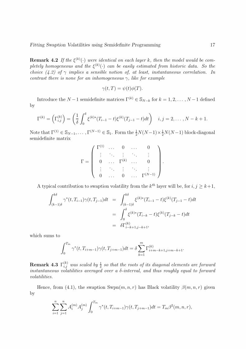
Remark 4.2 If the ξ(k)(·) were identical on each layer k, then the model would be com-pletely homogeneous and the ξ(k)(·) can be easily estimated from historic data. So thechoice (4.2) of γ implies a sensible notion of, at least, instantaneous correlation. Incontrast there is none for an inhomogeneous γ, like for example

γ(t, T ) = ψ(t)φ(T ).

Introduce the N−1 semidefinite matrices Γ(k) ∈ SN−k for k = 1, 2, . . . , N−1 definedby

Γ(k) =(Γ

(k)i,j

)=

(1

δ

∫ δ

0

ξ(k)∗(Ti−1 − t)ξ(k)(Tj−1 − t)dt

)i, j = 2, . . . , N − k + 1.

Note that Γ(1) ∈ SN−1, . . . ,Γ(N−1) ∈ S1. Form the 1

2N(N−1)× 1

2N(N−1) block-diagonal

semidefinite matrix

Γ =

Γ(1) . . . 0 . . . 0...

. . ....

. . ....

0 . . . Γ(k) . . . 0...

. . ....

. . ....

0 . . . 0 . . . Γ(N−1)

.

A typical contribution to swaption volatility from the kth layer will be, for i, j ≥ k+1,∫ kδ

(k−1)δ

γ∗(t, Ti−1)γ(t, Tj−1)dt =

∫ kδ

(k−1)δ

ξ(k)∗(Ti−1 − t)ξ(k)(Tj−1 − t)dt

=

∫ δ

0

ξ(k)∗(Ti−k − t)ξ(k)(Tj−k − t)dt

= δΓ(k)i−k+1,j−k+1,

which sums to∫ Tm

0

γ∗(t, Ti+m−1)γ(t, Tj+m−1)dt = δ

m∑k=1

Γ(k)i+m−k+1,j+m−k+1.

Remark 4.3 Γ(k)i,j was scaled by 1

δso that the roots of its diagonal elements are forward

instantaneous volatilities averaged over a δ-interval, and thus roughly equal to forwardvolatilities.

Hence, from (4.1), the swaption Swpn(m,n, r) has Black volatility β(m,n, r) givenby

n∑i=1

n∑j=1

A(m)i A

(m)j

∫ Tm

0

γ∗(t, Ti+m−1)γ(t, Tj+m−1)dt = Tmβ2(m,n, r),


leading to the equality constraint

n∑i=1

n∑j=1

m∑k=1

1

mA

(m)i A

(m)j Γ

(k)i+m−k+1,j+m−k+1 = β2(m,n, r). (4.3)

This constraint can be rewritten as the Frobenius product

u(m) • Γ = b(m), (4.4)

where the 12N(N − 1) × 1

2N(N − 1) constraint matrices u(m) are formed from the A

(m)i

according to (4.3).

4.3 Simplification

To fit a full quarterly volatility spectrum with time to maturity plus length of underlyingranging up to 10 years requires N = 40, making Γ a 780 × 780 matrix. That is acomputationally expensive problem for a 300 MHz laptop, despite the block structure ofΓ! So we “compact” our matrices into annual blocks and hence reduce the scale of theproblem by a factor of 4.

Specifically, introduce the nine (11−K)× (11−K) matrices Γ(K), for K = 1, . . . , 9,defined by

Γ(k)i,j = X

(K)I,J whenever (4.5)

i = 4(I − 1) + α, j = 4(J − 1) + β, k = 4(K − 1) + γ,

for I, J = 1, . . . , 11−K, and α, β, γ = 1, . . . , 4.

Because both the constraints (4.3) and “compaction” (4.5) are linear, clearly (4.4)can be rewritten in the form

U (m) •X = b(m), (4.6)

where X is the (now more computationally tractable) 54×54 block-diagonal semidefinitematrix defined by

X =

X(1) . . . 0 . . . 0

.... . .

.... . .

...0 . . . X(K) . . . 0...

. . ....

. . ....

0 . . . 0 . . . X(9)

,

and the U (m) are obtained by “compacting” the u(m). We can regard each successiveblock X(K) as the covariance of the Kth annual layer.


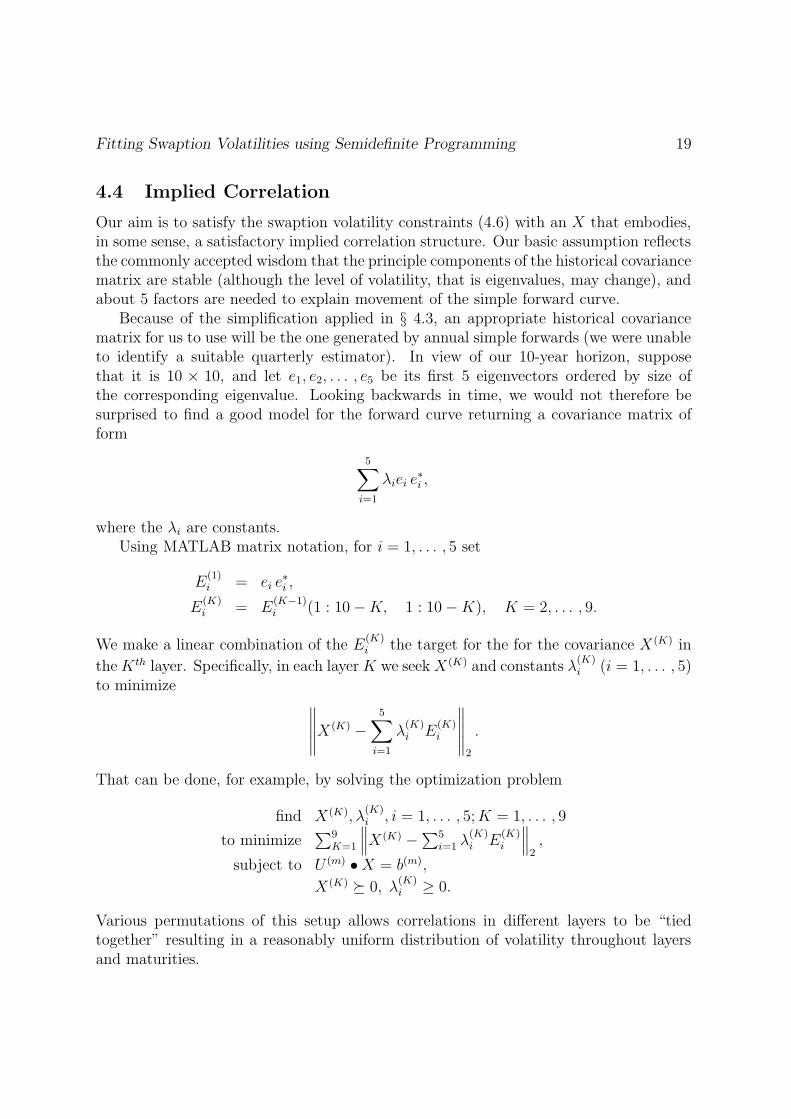
4.4 Implied Correlation

Our aim is to satisfy the swaption volatility constraints (4.6) with an X that embodies,in some sense, a satisfactory implied correlation structure. Our basic assumption reflectsthe commonly accepted wisdom that the principle components of the historical covariancematrix are stable (although the level of volatility, that is eigenvalues, may change), andabout 5 factors are needed to explain movement of the simple forward curve.

Because of the simplification applied in § 4.3, an appropriate historical covariancematrix for us to use will be the one generated by annual simple forwards (we were unableto identify a suitable quarterly estimator). In view of our 10-year horizon, supposethat it is 10 × 10, and let e1, e2, . . . , e5 be its first 5 eigenvectors ordered by size ofthe corresponding eigenvalue. Looking backwards in time, we would not therefore besurprised to find a good model for the forward curve returning a covariance matrix ofform

5∑i=1

λiei e∗i ,

where the λi are constants.Using MATLAB matrix notation, for i = 1, . . . , 5 set

E(1)i = ei e

∗i ,

E(K)i = E

(K−1)i (1 : 10−K, 1 : 10−K), K = 2, . . . , 9.

We make a linear combination of the E(K)i the target for the for the covariance X(K) in

theKth layer. Specifically, in each layerK we seekX(K) and constants λ(K)i (i = 1, . . . , 5)

to minimize ∥∥∥∥∥X(K) −5∑

i=1

λ(K)i E

(K)i

∥∥∥∥∥2

.

That can be done, for example, by solving the optimization problem

find X(K), λ(K)i , i = 1, . . . , 5;K = 1, . . . , 9

to minimize∑9

K=1

∥∥∥X(K) −∑5i=1 λ

(K)i E

(K)i

∥∥∥2,

subject to U (m) •X = b(m),

X(K) � 0, λ(K)i ≥ 0.

Various permutations of this setup allows correlations in different layers to be “tiedtogether” resulting in a reasonably uniform distribution of volatility throughout layersand maturities.


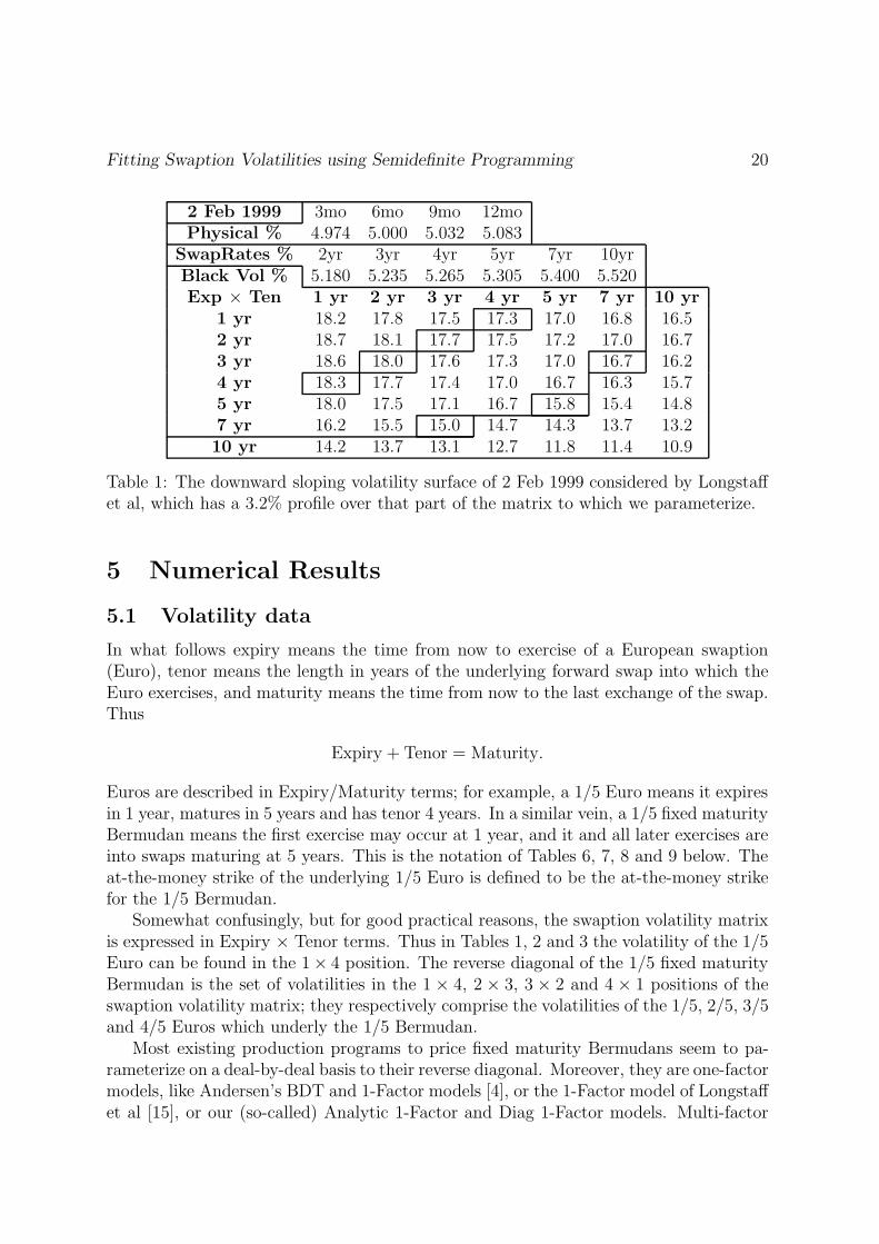
2 Feb 1999 3mo 6mo 9mo 12moPhysical % 4.974 5.000 5.032 5.083

SwapRates % 2yr 3yr 4yr 5yr 7yr 10yrBlack Vol % 5.180 5.235 5.265 5.305 5.400 5.520Exp × Ten 1 yr 2 yr 3 yr 4 yr 5 yr 7 yr 10 yr

1 yr 18.2 17.8 17.5 17.3 17.0 16.8 16.52 yr 18.7 18.1 17.7 17.5 17.2 17.0 16.73 yr 18.6 18.0 17.6 17.3 17.0 16.7 16.24 yr 18.3 17.7 17.4 17.0 16.7 16.3 15.75 yr 18.0 17.5 17.1 16.7 15.8 15.4 14.87 yr 16.2 15.5 15.0 14.7 14.3 13.7 13.210 yr 14.2 13.7 13.1 12.7 11.8 11.4 10.9

Table 1: The downward sloping volatility surface of 2 Feb 1999 considered by Longstaffet al, which has a 3.2% profile over that part of the matrix to which we parameterize.

5 Numerical Results

5.1 Volatility data

In what follows expiry means the time from now to exercise of a European swaption(Euro), tenor means the length in years of the underlying forward swap into which theEuro exercises, and maturity means the time from now to the last exchange of the swap.Thus

Expiry + Tenor = Maturity.

Euros are described in Expiry/Maturity terms; for example, a 1/5 Euro means it expiresin 1 year, matures in 5 years and has tenor 4 years. In a similar vein, a 1/5 fixed maturityBermudan means the first exercise may occur at 1 year, and it and all later exercises areinto swaps maturing at 5 years. This is the notation of Tables 6, 7, 8 and 9 below. Theat-the-money strike of the underlying 1/5 Euro is defined to be the at-the-money strikefor the 1/5 Bermudan.

Somewhat confusingly, but for good practical reasons, the swaption volatility matrixis expressed in Expiry × Tenor terms. Thus in Tables 1, 2 and 3 the volatility of the 1/5Euro can be found in the 1× 4 position. The reverse diagonal of the 1/5 fixed maturityBermudan is the set of volatilities in the 1 × 4, 2 × 3, 3 × 2 and 4 × 1 positions of theswaption volatility matrix; they respectively comprise the volatilities of the 1/5, 2/5, 3/5and 4/5 Euros which underly the 1/5 Bermudan.

Most existing production programs to price fixed maturity Bermudans seem to pa-rameterize on a deal-by-deal basis to their reverse diagonal. Moreover, they are one-factormodels, like Andersen’s BDT and 1-Factor models [4], or the 1-Factor model of Longstaffet al [15], or our (so-called) Analytic 1-Factor and Diag 1-Factor models. Multi-factor


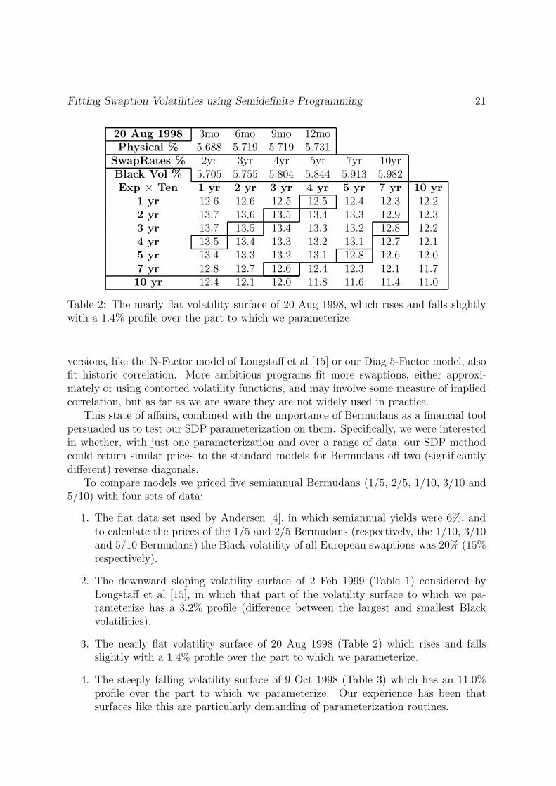
20 Aug 1998 3mo 6mo 9mo 12moPhysical % 5.688 5.719 5.719 5.731


1 yr 12.6 12.6 12.5 12.5 12.4 12.3 12.22 yr 13.7 13.6 13.5 13.4 13.3 12.9 12.33 yr 13.7 13.5 13.4 13.3 13.2 12.8 12.24 yr 13.5 13.4 13.3 13.2 13.1 12.7 12.15 yr 13.4 13.3 13.2 13.1 12.8 12.6 12.07 yr 12.8 12.7 12.6 12.4 12.3 12.1 11.710 yr 12.4 12.1 12.0 11.8 11.6 11.4 11.0

Table 2: The nearly flat volatility surface of 20 Aug 1998, which rises and falls slightlywith a 1.4% profile over the part to which we parameterize.

versions, like the N-Factor model of Longstaff et al [15] or our Diag 5-Factor model, alsofit historic correlation. More ambitious programs fit more swaptions, either approxi-mately or using contorted volatility functions, and may involve some measure of impliedcorrelation, but as far as we are aware they are not widely used in practice.

This state of affairs, combined with the importance of Bermudans as a financial toolpersuaded us to test our SDP parameterization on them. Specifically, we were interestedin whether, with just one parameterization and over a range of data, our SDP methodcould return similar prices to the standard models for Bermudans off two (significantlydifferent) reverse diagonals.

To compare models we priced five semiannual Bermudans (1/5, 2/5, 1/10, 3/10 and5/10) with four sets of data:

1. The flat data set used by Andersen [4], in which semiannual yields were 6%, andto calculate the prices of the 1/5 and 2/5 Bermudans (respectively, the 1/10, 3/10and 5/10 Bermudans) the Black volatility of all European swaptions was 20% (15%respectively).

2. The downward sloping volatility surface of 2 Feb 1999 (Table 1) considered byLongstaff et al [15], in which that part of the volatility surface to which we pa-rameterize has a 3.2% profile (difference between the largest and smallest Blackvolatilities).

3. The nearly flat volatility surface of 20 Aug 1998 (Table 2) which rises and fallsslightly with a 1.4% profile over the part to which we parameterize.

4. The steeply falling volatility surface of 9 Oct 1998 (Table 3) which has an 11.0%profile over the part to which we parameterize. Our experience has been thatsurfaces like this are particularly demanding of parameterization routines.


9 Oct 1998 3mo 6mo 9mo 12moPhysical % 5.344 5.152 5.000 4.938


1 yr 26.0 24.0 23.0 22.5 21.5 20.5 19.02 yr 23.0 22.0 21.0 19.3 18.8 18.0 17.53 yr 21.7 19.3 18.9 17.7 17.0 16.5 15.54 yr 19.2 18.1 17.0 16.3 15.6 15.2 14.15 yr 18.0 17.2 16.2 15.5 15.0 14.2 13.27 yr 16.0 15.5 15.0 14.5 14.0 13.0 11.710 yr 14.1 13.0 12.4 11.4 10.6 10.0 9.2

Table 3: The steeply falling volatility surface of 9 Oct 1998, which has an 11.0% profileover the part to which we parameterize.

Tables 1,2, 3 contain input data from the US taken off Bloomberg for the three days 2Feb 99, 20 Aug 98 and 9 Oct 98. Swaprates are semi-annual, the daycount for both cashand swaprates is Actual/360, and volatilities are percentage Black semiannual swaptionvolatilities.

Generally volatility surfaces either rise and fall or just fall, rarely do they uniformlyrise. Moreover the 1/5, 2/5 and 1/10, 3/10, 5/10 reverse diagonals are fairly widelyseparated. So we feel that, while more comparisons might be better, our choice of dataand Bermudan maturities ought to constitute a robust and revealing test.

The models used by Andersen and Longstaff et al are described in their papers [4]and [15] respectively. The volatility function in our Analytic 1-Factor and Diag 1-Factormodels depends only on maturity; the former splines values on nodes and numericallyintegrates down through the exercise times (hence the name “Analytic”), while the lattercombines the simulation techniques of Glasserman et al [9] with the Bermudan techniquesof Longstaff et al [14]. The volatility function in the Diag 5-Factor model dependsmainly on maturity, but also incorporates a homogeneous multi-factor component tocarry historical correlation.

5.2 Covariance approximation

Table 4 specifies our covariance matrix. Annual forwards were used because we felt theircovariance best corresponded to the way we “compacted” our matrices and volatilityfunctions from quarterly to annual periods in order to get a computationally simpleenough problem for our SDP software to tackle (we were also unable to find a betterestimator).

Targeting actual historic correlation via the SDP objective function is not possiblebecause the problem is non-linear. So we fell back on what seems to be part of the folk


1 yr 2 yr 3 yr 4 yr 5 yr 6 yr 7 yr 8 yr 9 yr 10 yr2.392 2.696 2.564 2.365 2.189 2.038 1.913 1.810 1.729 1.668 1 yr

3.760 3.834 3.634 3.413 3.229 3.086 2.975 2.889 2.825 2 yr4.094 3.976 3.780 3.602 3.462 3.357 3.280 3.226 3 yr

3.945 3.810 3.662 3.529 3.428 3.360 3.317 4 yr3.745 3.641 3.526 3.433 3.373 3.341 5 yr

3.590 3.522 3.461 3.421 3.397 6 yr3.518 3.510 3.497 3.480 7 yr

3.547 3.561 3.555 8 yr3.596 3.603 9 yr

3.625 10 yr

Table 4: 100 times the annualized historical covariance matrix for annual forwards,computed from data running from May 1994 to Feb 2000.

Total = 371 < 20% < 30% > 30% > 50% > 70% > 100%Flat 15% 371 371 0 0 0 0

2 Feb 1999 323 365 6 0 0 020 Aug 1998 363 371 0 0 0 09 Oct 1998 279 313 58 26 8 0

Table 5: Number of elements, out of a total of 371, whose absolute percentage differencesbetween implied and target correlations lie in the given ranges, for the four data sets.

wisdom of financial mathematics (we have no references), that the shapes of the largest(ranked by eigenvalue) eigenvectors of the historical covariance matrix are invariant. Inour SDP routine we minimize the matrix 2-norm of the difference between the covariancematrix we are seeking, and a target covariance matrix formed by any linear combinationof the first five eigenvectors times their transposes, of the historic covariance.

Thus the correlations implied by our fitted covariances approximate the correlationsdetermined by the target covariance, which in turn approximate actual historic corre-lations. Experiments, in which we changed eigenvalues but not eigenvectors, convincedus that absolute differences of up to 30% between corresponding elements of correlationmatrices related in this way, generally make little difference in practice. So we believe agood covariance fit simultaneously gets all elements of the implied correlation matrices towithin 30% of corresponding correlations derived from the target, and pointedly ignorethe actual historic correlation matrix. Our dilemma arises, of course, from the existenceof two appealing but incompatible notions of “good correlation fit”, only one of whichsuits the SDP framework. The results of our covariance fit are contained in Table 5.

We have not analyzed implied correlation extensively, but despite the many unan-swered questions that occur to us, some comments can be made. Some 371 comparisonsare possible between elements in the implied correlation matrices and corresponding el-


Flat Case Exp/Mat 1/5 2/5 1/10 3/10 5/10Black Volatility 20% 20% 15% 15% 15%

European Black 158.1 162.4 232.5 293.3 253.6Payer SDP 5-Factor 157.7

(0.8)162.0(0.8)

231.8(1.1)

291.1(1.4)

251.7(1.3)

Bermudan Analytic 1-Factor 220.0 188.9 411.7 369.2 284.2Payer Andersen 1-Factor - - - 187.9 - - - - - - 282.7

Andersen BDT - - - 187.8 - - - - - - 283.8Diag 1-Factor 217.9

(0.4)187.6(0.4)

401.2(0.7)

365.4(0.7)

282.6(0.6)

Diag 5-Factor 221.8(0.4)

190.6(0.4)

412.6(0.7)

371.5(0.7)

287.0(0.6)

SDP 5-Factor 214.3(0.8)

185.6(0.8)

400.2(1.4)

360.8(1.4)

279.2(1.2)

European Black 158.1 162.4 232.5 293.3 253.6Receiver SDP 5-Factor 157.7

(0.7)161.7(0.7)

232.5(1.0)

292.6(1.3)

252.6(1.1)

Bermudan Analytic 1-Factor 217.6 187.4 400.7 361.8 280.8Receiver Andersen 1-Factor - - - 186.6 - - - - - - 279.5

Andersen BDT - - - 186.8 - - - - - - 279.2Diag 1-Factor 215.9

(0.3)186.6(0.3)

397.6(0.5)

359.5(0.5)

280.0(0.5)


188.4(0.3)

401.3(0.5)

361.8(0.5)

281.8(0.4)

SDP 5-Factor 212.7(0.7)

183.8(0.6)

395.6(1.2)

357.7(1.2)

277.5(1.0)

Table 6: Bermudan and Euro prices in the flat case. Numbers which strike us as inter-esting have been rendered bold.

ements in the target correlation matrices. Listed in Table 5 are the numbers of elementswhose absolute percentage difference falls in the indicated category. By our criteria,clearly the Flat and 20 Aug 98 fits can be regarded as good, the 2 Feb 99 as satisfactory,and the 9 Oct 98 fit as poor. All efforts to significantly improve the last fit failed, sowe feel that the result reflects reality: when the volatility surface slopes steeply down,implied correlation moves sharply away from historical correlation.

5.3 Bermudan prices

Our Analytic and Diag models were parameterized on a deal-by-deal basis to the reversediagonal of the Bermudan being considered. To price the 1/5 and 2/5 Bermudans weparameterized to the 1/5, 2/5, 3/5 and 4/5 Euros, whose volatilities are boxed in Tables1, 2 and 3. To price the 1/10, 3/10 and 5/10 Bermudans we parameterized to 3/10,5/10 and 7/10 Euros (volatilities boxed), and also to the 1/10, 2/10, 4/10, 6/10, 8/10and 9/10 Euros by linearly interpolating their unspecified volatilities off the tables. OurSDP routine parameterized to those 31 Euros, with maturity less than or equal to 10


2 Feb 1999 Exp/Mat 1/5 2/5 1/10 3/10 5/10European Black 127.1 134.4 249.8 323.2 270.9Payer SDP 5-Factor 127.3

(0.6)134.8(0.7)

251.5(1.2)

321.6(1.6)

269.1(1.4)

Bermudan Analytic 1-Factor 181.6 158.0 474.3 418.4 307.9Payer Longstaff 1-Factor 179.7 157.0 466.1 411.3 304.1


157.7(0.4)

463.7(0.7)

415.0(0.8)

309.4(0.7)

Longstaff N-Factor 189.7 164.9 500.4 439.1 322.3Diag 5-Factor 182.4

(0.3)159.5(0.4)

473.9(0.8)

421.8(0.8)

313.5(0.7)

SDP 5-Factor 183.8(0.7)

161.2(0.7)

460.5(1.6)

407.2(1.6)

314.0(1.4)


(0.5)134.8(0.6)

252.5(1.1)

322.6(1.4)

271.2(1.1)

Bermudan Analytic 1-Factor 175.4 154.8 409.8 383.6 295.8Receiver Longstaff 1-Factor 175.5 154.3 412.7 386.7 295.1


155.0(0.2)

407.9(0.5)

382.2(0.6)

299.2(0.5)

Longstaff N-Factor 181.9 159.6 431.1 401.5 305.3Diag 5-Factor 175.6

(0.2)155.7(0.2)

409.8(0.5)

383.9(0.6)

300.1(0.5)

SDP 5-Factor 176.1(0.6)

156.6(0.5)

404.0(1.3)

374.3(1.3)

301.0(1.1)

Table 7: Bermudan and Euro prices for the downward sloping volatility surface con-sidered by Longstaff et al. Numbers which strike us as interesting have been renderedbold

years, which appear above the lower stepped line in the tables.Our results are contained in Tables 6, 7, 8 and 9 which list the prices of at-the-

money semi-annual European and Bermudan options in points–per–million ($100 unitsper $1,000,000 face value) for each of our four data sets.

In a separate exercise to back check each parameterization (not tabulated), at-the-money values of the 31 fitted Euros were simulated; in all cases values returned werewithin two standard deviations of the corresponding Black value. Those 31 Euros includethe 1/5, 2/5, 3/10, 5/10 Euros, so our simulated European prices in Tables 6–9 oughtto agree with the Black prices. They do, with the exception of the 3/10 EuropeanPayer in Table 9 which we regard as a statistically acceptable anomaly. So our SDPparameterization successfully returns fitted options.

To our surprise, Burmudan prices produced by the SDP parameterizations were eitherroughly equal to, or less than, prices from the single factor models. In particular, pricesof the “real Bermudan” 1/10s (the 5/10s are “half vanilla”) were almost uniformly lower,and in the case of the 1/10 Payer of 9 Oct 1998 significantly so (40-50 points or around9% of value). This finding contrasts with the view of Longstaff et. al [15] who believe


20 Aug 1998 Exp/Mat 1/5 2/5 1/10 3/10 5/10European Black 99.0 110.9 192.9 258.5 225.2Payer SDP 5-Factor 99.2

(0.5)110.2(0.6)

190.3(0.9)

257.7(1.3)

225.1(1.1)

Bermudan Analytic 1-Factor 147.8 130.8 373.6 332.4 253.6Payer Diag 1-Factor 147.0

(0.2)130.5(0.3)

366.6(0.6)

329.4(0.6)

253.6(0.6)


132.0(0.3)

373.5(0.6)

334.7(0.6)

257.3(0.6)

SDP 5-Factor 150.2(0.6)

129.2(0.6)

371.7(1.3)

329.3(1.3)

254.7(1.1)


(0.4)110.1(0.5)

190.8(0.9)

257.9(1.1)

226.0(1.0)

Bermudan Analytic 1-Factor 136.1 126.5 328.3 315.8 248.0Receiver Diag 1-Factor 135.4

(0.5)126.6(0.2)

327.1(0.4)

314.7(0.5)

249.9(0.4)


127.2(0.2)

329.2(0.4)

316.4(0.5)

250.4(0.4)

SDP 5-Factor 137.6(0.5)

124.7(0.5)

327.3(1.0)

312.4(1.1)

249.1(0.9)

Table 8: Bermudan and Euro prices for a fairly flat volatility surface. Numbers whichstrike us as interesting have been rendered bold.

single factor models underprice Bermudans.We are uncertain just what to make of our results. Our experience with the Diag

5-Factor model was that one could shift prices 20-30 points by massaging correlation;tight fits of forwards to cash and swap rates produced lumpy unstable eigenvectors andhigher prices, while looser fits produced smoother more stable eigenvectors and lowerprices. Perhaps there is some roughly similar effect, not yet clear to us, that works inthe opposite direction for our SDP parameterizations.

Nevertheless, we take comfort from the fact that Bermudans have been priced withsingle factor models for a long time, with only a couple (as far as we know) of rumouredinstances of significant writeoffs. Because banks tend to be overall buyers of Bermudans,such writeoffs would likely arise from models that overprice rather than underprice.These thoughts combine to favour our findings.

References

[1] Alizadeh, F., J. P. Haeberly, M. V. Nayakkankuppam, M. L. Overton, and S. Schmi-eta, (1997): “SDPPACK User’s Guide, Version 0.9 Beta for MATLAB 5.0.”http://cs.nyu.edu/cs/faculty/overton/sdppack/sdppack.html

[2] Alizadeh, F., J. P. Haeberly, and M. L. Overton (1998): “Primal-dual interior-pointmethods for semidefinite programming: convergence rates, stability and numerical


9 Oct 1998 Exp/Mat 1/5 2/5 1/10 3/10 5/10European Black 158.3 159.3 290.9 327.0 263.4Payer SDP 5-Factor 159.1

(0.8)158.9(0.8)

294.9(1.4)

330.6(1.6)

264.3(1.4)

Bermudan Analytic 1-Factor 243.9 194.4 550.4 425.7 302.7Payer Diag 1-Factor 243.2

(0.4)195.2(0.4)

542.4(0.7)

423.4(0.7)

303.0(0.6)


198.0(0.4)

558.0(0.8)

431.2(0.8)

307.0(0.7)

SDP 5-Factor 237.9(0.9)

194.5(0.8)

506.4(1.8)

413.2(1.7)

312.9(1.3)


(0.7)160.4(0.7)

297.5(1.3)

326.7(1.4)

265.1(1.1)

Bermudan Analytic 1-Factor 195.4 175.2 410.2 379.4 286.9Receiver Diag 1-Factor 195.4

(0.3)177.0(0.3)

410.3(0.6)

378.4(0.6)

288.6(0.5)


177.6(0.3)

411.3(0.6)

380.5(0.6)

289.3(0.5)

SDP 5-Factor 188.2(0.7)

173.7(0.6)

386.9(1.3)

370.2(1.3)

295.1(1.1)

Table 9: Bermudan prices for the steeply falling volatility surface. Numbers which strikeus as interesting have been rendered bold.

results”, SIAM Journal on Optimization, 8, 746–768.

[3] Andersen, L. and J. Andreasen (1998): “Volatility skews and extensions of the Libormarket model”, General Re Financial Products Working Paper, August 1998.

[4] Andersen, L. (1999): “A simple approach to the pricing of Bermudan swaptionsin the multi-factor Libor market model”, General Re Financial Products WorkingPaper, March 1999.

[5] Boyd, S., L. E. Ghaoui, E. Feron, and V. Balakrishnan (1994): Linear MatrixInequalities in System and Control Theory, SIAM, Philadelphia.

[6] Brace A., T. Dun and G. Barton (1998): “Towards a Central Interest Rate Model”,ICBI Global Derivatives Conference, Paris, April 1998.

[7] Barton, G., T. Dun and E. Schloegl (2000): “Simulated swaption delta hedging inthe lognormal forward Libor model”, University Technology Sydney working paper,February 2000.

[8] Brace, A., D. Gatarek and M. Musiela (1997): “The market model of interest ratedynamics”, Mathematical Finance 7, 127–155.


[9] Glasserman, P. and X.L. Zhao (1998): “Arbitrage-free discretization of lognor-mal forward Libor and swaprate models”, Columbia Business School working paperFebruary 1998.

[10] Golub, G. and C. Van Loan (1996): Matrix Computations, 3rd edition, John Hop-kins University Press, Baltimore and London.

[11] Helmberg, C., F. Rendl, R. Vanderbei, and H. Wolkowicz (1996): “An interiorpoint method for semi-definite programming”, SIAM Journal on Optimization, 6,342–361.

[12] Horn, R. A. and C. R. Johnson (1985): Matrix Analysis, Cambridge UniversityPress, Cambridge.

[13] Lewis, A. S. and M. L. Overton, eds. (1996): “Eigenvalue optimization,” ACTANumerica, 149–190.

[14] Longstaff, F. A. and E.S. Schwartz (1998): “Valuing American options by simula-tion: A simple least squares approach”, Anderson School at UCLA Working Paper,October 1998.

[15] Longstaff, F. A., P. Santa-Clara, and E.S. Schwartz (1999): “Throwing away abillion dollars: the cost of suboptimal exercise strategies in the swaptions market”,Anderson School at UCLA working paper, May 1999.

[16] Muirhead, R. J. (1982): Aspects of Multivariate Statistical Theory, John Wiley,Chichester and New York.

[17] Musiela, M. and M. Rutkowski (1997): Martingale Methods in Financial Modelling,Springer-Verlag.

[18] Musiela, M. and M. Rutkowski (1997): “Continuous-time term structure models:forward measure approach,” Finance and Stochastics 1, 261-291.

[19] Nesterov, Y. and A. Nemirovski (1994): Interior Point Polynomial Methods in Con-vex Programming, SIAM, Philadelphia.

[20] Overton M. L. and H. Wolkowic (1997): “Semidefinite programming,” MathematicalProgramming, 77, 105–110.

[21] Pedersen, M. B. (1999): “Bermudan swaptions in the Libor market model,” Sim-Corp Financial Research Working Paper, March 1999.

[22] Sturm J. F. (1999): “Using SeDuMi 1.02, a MATLAB toolbox for optimization oversymmetric cones,” Department of Quantitative Economics, Maastricht University,Netherlands, http://www.unimaas.nl/~sturm.


[23] Vandenberghe, L. and S. Boyd (1996): “Semidefinite programming,” SIAM Review,38, 49–95.

[24] Wright, S. (1997): Primal-Dual Interior-Point Methods, SIAM, Philadelphia.

[25] Wolkowicz, H., R. Saigal and L. Vandenberghe eds. (2000): Handbook on Semidef-inite Programming, Kluwer.

exact fit to the swaption volatility matrix using semide...

Documents