exact likelihood inference for laplace distribution based ... · exact likelihood inference for...

Exact likelihood inference for Laplace distribution

based on Type-II censored samples

G. Iliopoulos∗ and N. Balakrishnan†

Abstract

We develop exact inference for the location and scale parameters of the Laplace (double ex-ponential) distribution based on their maximum likelihood estimators from a Type-II censoredsample. Based on some pivotal quantities, exact confidence intervals and tests of hypothesesare constructed. Upon conditioning first on the number of observations that are below the pop-ulation median, exact distributions of the pivotal quantities are expressed as mixtures of linearcombinations and of ratios of linear combinations of standard exponential random variables,which facilitates the computation of quantiles of these pivotal quantities. Tables of quantilesare presented for the complete sample case.

AMS 2010 subject classifications: Primary 62E15; Secondary 62F03, 62F10.

Keywords and phrases: Laplace (double exponential) distribution; exact inference; maximum

likelihood estimators; Type-II censoring; mixtures; pivotal quantities; linear combinations of expo-

nential order statistics.

1 Introduction

Let X1, . . . ,Xn, n > 2, be a random sample from the Laplace (or double exponential) distribution

L(µ, σ), µ ∈ R, σ > 0, with probability density function (pdf)

f(x;µ, σ) =1

2σe−

1

σ|x−µ|, x ∈ R.

It is well-known (see, for example, Johnson et al., 1995, and Kotz et al., 2001) that the maximum

likelihood estimators (MLEs) µ and σ of µ and σ are the sample median and the sample mean

deviation from the sample median, respectively. Note that in the case of an even sample size, µ

is not unique since then any point between the two middle observations maximizes the likelihood

function with respect to µ. However, it is customary to define the sample median as the average

of the two middle observations and take that as the MLE of µ, and that is what we will do too

∗Department of Statistics and Insurance Science, University of Piraeus, 80 Karaoli & Dimitriou str., 18534 Piraeus,

Greece; e–mail: [email protected]†Department of Mathematics and Statistics, McMaster University, Hamilton, Ontario, Canada L8S 4K1; e–mail:

[email protected]

1

hereafter. On the other hand, σ is always well-defined, since it turns out to be the difference of

the sum of all sample points above µ (whatever we take it to be) and the sum of all sample points

below µ divided by the sample size.

Balakrishnan and Cutler (1995) showed that the MLEs can be explicitly derived even in the

presence of general Type-II censoring in the sample. Their result was further generalized by Childs

and Balakrishnan (1997). To be more specific, let X1:n < · · · < Xn:n denote the ordered sample

and assume that r observations have been censored from the left and s observations have been

censored from the right, i.e., the observed data consist of the order statistics

Xr+1:n < · · · < Xn−s:n,

which corresponds to a doubly Type-II censored sample. Such a censored sample may arise ei-

ther naturally (for example, when some extreme values cannot be recorded due to experimental

constraints or they are just missing) or intentionally (when the researcher decides to ignore some

extreme observations based on robustness considerations). In order to be able to estimate both

parameters, at least two observations are needed and so, we will assume that n−r−s > 2. Clearly,

when r = s = 0, the complete data are observed. In what follows, m = m(n) > 1 is defined to be

equal to (n+1)/2 when n is odd and n/2 when n is even. In other words, we are taking n = 2m−1

and n = 2m for the odd and even sample cases, respectively. Then, from the above mentioned

works, the following expressions of the MLEs are known:

• If max(r, s) < m, then

µ =

{

Xm:n, n = 2m − 112 (Xm:n + Xm+1:n), n = 2m,

i.e., the sample median, and

σ =1

n − r − s

{ n−s∑

i=m+1

Xi:n + sXn−s:n − rXr+1:n −

[n/2]∑

i=r+1

Xi:n

}

,

where [x] denotes the integer part of x, and by convention∑ℓ

i=k ≡ 0 when k > ℓ;

• if s > m, then

σ =1

n − r − s

{ n−s∑

i=r+1

(Xn−s:n − Xi:n) + r(Xn−s:n − Xr+1:n)

}

and

µ = Xn−s:n + log

(

n/2

n − s

)

σ;

2

• if r > m, then

σ =1

n − r − s

{ n−s∑

i=r+1

(Xi:n − Xr+1:n) + s(Xn−s:n − Xr+1:n)

}

and

µ = Xr+1:n + log

(

n − r

n/2

)

σ.

Since µ and σ are the location and scale parameters, respectively, it is evident that the random

variables T = (µ − µ)/σ and S = σ/σ have distributions which are free of both parameters and

can therefore serve as pivotal quantities. Hence, inference about µ and σ can be carried out based

on T and S, respectively. Indeed, Bain and Engelhardt (1973) considered approximate inference

based on the above pivotal quantities. Kappenman (1975) subsequently developed conditional

inference for µ and σ by conditioning on appropriate ancillary statistics. Grice, Bain and Engelhardt

(1978) compared numerically the two approaches with respect to inference about µ and found that

the conditional one gives slightly narrower confidence intervals. Childs and Balakrishnan (1996)

extended Kappenman’s (1975) conditional approach to the case of Type-II right censored data. A

completely different procedure based on the distribution of the standard t-statistic in the Laplace

case was considered by Sansing (1976).

In this paper, we develop exact inference for µ and σ based on T and S either when the sample

is complete or when it is general Type-II censored. The importance of the results established here is

two-fold. First, we provide the necessary tools for constructing exact confidence intervals and tests

of hypotheses under the important Laplace model that often serves as an alternative to the normal

distribution; see Kotz et al. (2001). Moreover, by tabulating the most commonly used quantiles of

T and S (see Tables 4 and 5), we make these inferential processes as straightforward as in the case

of normal samples. Secondly, exact inferential methods under censoring developed under Laplace

model makes a substantial addition as there are very few models such as exponential, Pareto and

uniform for which this development is possible.

The rest of this paper is organized as follows. In Section 2, we describe some known preliminary

results on the Laplace distribution and also on the conditional distributions of order statistics which

are essential for the ensuing developments. In Sections 3 and 4, we derive the exact distributions

of S and T , respectively. We show that S is distributed as a mixture of linear combinations of

independent standard exponential random variables while T is distributed as a mixture of ratios

of (dependent) linear combinations of independent standard exponential random variables. Using

these distributional results, in Section 5, we develop exact confidence intervals and tests of hy-

potheses about the parameters µ and σ. We also evaluate the performance of confidence intervals

3

obtained from an asymptotic approach given by Bain and Engelhardt (1973) and from the para-

metric bootstrap approach. In Section 6, we use a real dataset as an example and illustrate all the

inferential procedures developed here. In Section 7, we make some concluding remarks. Finally, an

Appendix presents the derivations of all the above mentioned distributions of the pivotal quantities.

2 Preliminaries

Let X ∼ L(µ, σ). It is well-known that the parameter µ is the median of the distribution and thus,

P(X 6 µ) = P(X > µ) = 1/2. Moreover, the conditional distribution of X − µ, given X > µ, is

exponential with mean σ, denoted by E(σ). This is also the conditional distribution of µ−X, given

X 6 µ.

Let Z1, . . . , Zniid∼ E(σ) and denote by Z1:n < · · · < Zn:n the corresponding order statistics.

For i = 1, . . . , n, let us denote the i-th spacing Zi:n − Zi−1:n by Zi:n, where Z0:n ≡ 0. Then, the

normalized spacings

nZ1:n, (n − 1)Z2:n, · · · , (n − i + 1)Zi:n , · · · , Zn:n

form a random sample from E(σ) as well (see Arnold et al., 2008).

Iliopoulos and Balakrishnan (2009) established the following independence result concerning or-

der statistics. If X1, . . . ,Xn is a random sample from any (either discrete or continuous) parent dis-

tribution and D denotes the number of X’s being at most equal to a pre-fixed constant C, then, con-

ditional on D = d, the blocks of order statistics (X1:n, . . . ,Xd:n) and (Xd+1:n, . . . ,Xn:n) are indepen-

dent. Moreover, conditional on D = d, (X1:n, . . . ,Xd:n)d= (L1:d, . . . , Ld:d) and (Xd+1:n, . . . ,Xn:n)

d=

(R1:n−d, . . . , Rn−d:n−d), where L1, . . . , Ld is a random sample from the parent distribution right

truncated at C, and R1, . . . , Rn−d is a random sample from the parent distribution left truncated

at C.

Now, we shall explain how we can use the above results for the inferential problem at hand. Con-

sider the complete sample X1, . . . ,Xn from L(µ, σ) and set D = #{X ′s 6 µ}. Clearly, D follows a

binomial B(n, 1/2) distribution. Conditional on D = d, (µ − Xd:n, . . . , µ − X1:n)d= (L1:d, . . . , Ld:d)

and (Xd+1:n − µ, . . . ,Xn:n − µ)d= (R1:n−d, . . . , Rn−d:n−d), where L1, . . . , Ld, R1, . . . , Rn−d

iid∼ E(σ).

Moreover, since any linear combination of Li:d’s and Rj:n−d’s can be expressed as a linear combi-

nation of the spacings Li:d’s and Rj:n−d’s which are independent E(σ) random variables, we will

first condition on D = d and express S and T through linear combinations of the above spacings.

Then, we will derive the conditional distributions of S and T for all d = 0, 1, . . . , n, and finally

we will uncondition with respect to D in order to express the unconditional distributions of S

and T as suitable mixtures. It should be mentioned that this mixture representation of the exact

4

distributions of the MLEs, in the special case of complete samples of odd sizes, may be deduced

from Proposition 2.6.6 of Kotz et al. (2001).

3 The distribution of S = σ/σ

By invariance, the distribution of S does not depend on σ and so we may take σ = 1 without loss

of any generality. In what follows, we set D = #{X ′s 6 µ}. Moreover, let L1, . . . , Ln, R1, . . . , Rn

be iid E(1) random variables and V an independent gamma G(a, 1) random variable with scale

parameter 1 and shape parameter a which will be suitably determined later.

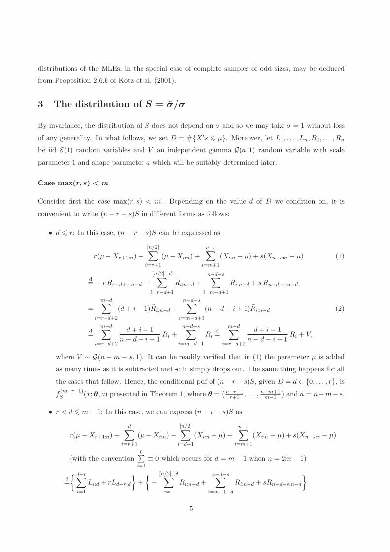
Case max(r, s) < m

Consider first the case max(r, s) < m. Depending on the value d of D we condition on, it is

convenient to write (n − r − s)S in different forms as follows:

• d 6 r: In this case, (n − r − s)S can be expressed as

r(µ − Xr+1:n) +

[n/2]∑

i=r+1

(µ − Xi:n) +

n−s∑

i=m+1

(Xi:n − µ) + s(Xn−s:n − µ) (1)

d= − r Rr−d+1:n−d −

[n/2]−d∑

i=r−d+1

Ri:n−d +n−d−s∑

i=m−d+1

Ri:n−d + s Rn−d−s:n−d

=

m−d∑

i=r−d+2

(d + i − 1)Ri:n−d +

n−d−s∑

i=m−d+1

(n − d − i + 1)Ri:n−d (2)

d=

m−d∑

i=r−d+2

d + i − 1

n − d − i + 1Ri +

n−d−s∑

i=m−d+1

Rid=

m−d∑

i=r−d+2

d + i − 1

n − d − i + 1Ri + V,

where V ∼ G(n − m − s, 1). It can be readily verified that in (1) the parameter µ is added

as many times as it is subtracted and so it simply drops out. The same thing happens for all

the cases that follow. Hence, the conditional pdf of (n− r − s)S, given D = d ∈ {0, . . . , r}, is

f(m−r−1)S (x;θ, a) presented in Theorem 1, where θ =

(

n−r−1r+1 , . . . , n−m+1

m−1

)

and a = n−m− s.

• r < d 6 m − 1: In this case, we can express (n − r − s)S as

r(µ − Xr+1:n) +

d∑

i=r+1

(µ − Xi:n) −

[n/2]∑

i=d+1

(Xi:n − µ) +

n−s∑

i=m+1

(Xi:n − µ) + s(Xn−s:n − µ)

(with the convention0∑

i=1≡ 0 which occurs for d = m − 1 when n = 2m − 1)

d=

{ d−r∑

i=1

Li:d + rLd−r:d

}

+

{

−

[n/2]−d∑

i=1

Ri:n−d +

n−d−s∑

i=m+1−d

Ri:n−d + sRn−d−s:n−d

}

5

=

{ d−r∑

i=1

(d − i + 1)Li:d

}

+

{ m−d∑

i=1

(d + i − 1)Ri:n−d +n−d−s∑

i=m−d+1

(n − d − i + 1)Ri:n−d

}

d=

d−r∑

i=1

Li +

m−d∑

i=1

d + i − 1

n − d − i + 1Ri +

n−d−s∑

i=m−d+1

Rid=

m−d∑

i=1

d + i − 1

n − d − i + 1Ri + V,

where V ∼ G(n − m − s − r + d, 1). Hence, (n − r − s)S|(D = d) ∼ f(m−d)S (x;θ, a), where

θ =(

n−dd , . . . , n−m+1

m−1

)

and a = n − m − s − r + d.

• d = m 6= n − s: In this case, we can express (n − r − s)S as

r(µ − Xr+1:n) +

[n/2]∑

i=r+1

(µ − Xi:n) +n−s∑

i=m+1

(Xi:n − µ) + s(Xn−s:n − µ)

d=

{ m−r∑

i=m−[n/2]+1

Li:m + r Lm−r:m

}

+

{ n−m−s∑

i=1

Ri:n−m + sRn−m−s:n−m

}

=

{

[n/2]L1:m +m−r∑

i=2

(m − i + 1)Li:m

}

+

{ n−m−s∑

i=1

(n − m − i + 1)Ri:n−m

}

d=

[n/2]

mL1 +

m−r∑

i=2

Li +

n−m−s∑

i=1

Rid=

[n/2]

mL1 + V,

where V ∼ G(n − s − r − 1, 1). Note that when n = 2m the above conditional distribution

becomes G(n − s − r, 1). Thus, (n − r − s)S|(D = m) ∼ f(1)S (x;θ, a), where θ =

(

mm−1

)

and

a = n − s − r − 1 when n = 2m − 1, or G(n − s − r, 1) when n = 2m.

• m + 1 6 d < n − s: Due to symmetry, (n − r − s)S has the same conditional distribution

either when we condition on D = d or on D = n − d. So, by interchanging d and n − d in

the conditional distribution of the case r < d 6 m − 1, we have (n − r − s)S|(D = d) ∼

f(m−n+d)S (x;θ, a), where θ =

(

dn−d , · · · , n−m+1

m−1

)

and a = 2n − m − r − s − d.

• n−s 6 d 6 n: Yet again, due to symmetry, the conditional distribution of (n−r−s)S, given

D = d, is f(m−s−1)S (x;θ, a), where θ =

(

n−s−1s+1 , · · · , n−m+1

m−1

)

and a = n − m − r.

Case s > m

• d 6 r: In this case, (n − r − s)S may be expressed as

− r(Xr+1:n − µ) −n−s∑

i=r+1

(Xi:n − µ) + (n − s)(Xn−s:n − µ)

d= − r Rr−d+1:n−d −

n−d−s∑

i=r−d+1

Ri:n−d + (n − s)Rn−d−s:n−d

6

=n−d−s∑

i=r−d+2

(d + i − 1)Ri:n−dd=

n−d−s∑

i=r−d+2

d + i − 1

n − d − i + 1Ri.

Hence, (n− r− s)S|(D = d) ∼ f(n−r−s−1)S (x;θ, a), where θ =

(

n−r−1r+1 , · · · , s+1

n−s−1

)

and a = 0.

• r + 1 6 d < n − s: In this case, we can express (n − r − s)S as

r(µ − Xr+1:n) +

d∑

i=r+1

(µ − Xi:n) −

n−s∑

i=d+1

(Xi:n − µ) + (n − s)(Xn−s:n − µ)

d=

{ d−r∑

i=1

Li:d + rLd−r:d

}

+

{

−n−d−s∑

i=1

Ri:n−d + (n − s)Rn−d−s:n−d

}

=

{ d−r∑

i=1

(d − i + 1)Li:d

}

+

{ n−d−s∑

i=1

(d + i − 1)Ri:n−d

}

d=

d−r∑

i=1

Li +

n−d−s∑

i=1

d + i − 1

n − d − i + 1Ri

d=

n−d−s∑

i=1

d + i − 1

n − d − i + 1Ri + V,

where V ∼ G(d − r, 1). Hence, (n − r − s)S|(D = d) ∼ f(n−d−s)S (x;θ, a), where θ =

(

n−dd , · · · , s+1

n−s−1

)

and a = d − r.

• d > n − s: Finally, in this case, (n − r − s)S can be expressed as

r(µ − Xr+1:n) +

n−s∑

i=r+1

(µ − Xi:n) − (n − s)(µ − Xn−s:n)

d=rLd−r:d +

d−r∑

i=d−n+s+1

Li:d − (n − s)Ld−n+s+1:d

=d−r∑

i=d−n+s+2

(d − i + 1)Li:dd=

n−r−s−1∑

i=1

Lid= V,

where V ∼ G(n − r − s − 1, 1). Hence, (n − r − s)S|(D = d) ∼ G(n − r − s − 1, 1).

Case r > m

Using again a symmetry argument, we conclude that the conditional distributions of (n − r − s)S,

given D = d, are as in the previous section when interchanging r and s, and replacing d by n − d.

Let f∗S|D(x|d) denote in general the conditional pdf of (n − r − s)S, given D = d. Then, by

standard arguments, the conditional pdf of S, given D = d, is fS|D(x|d) = (n− r− s)f∗S|D((n− r−

s)x|d). Using now all the conditional pdfs of S, given D = d, presented above, we can express the

exact pdf of S as

fS(x) =

n∑

d=0

P(D = d)fS|D(x|d) =1

2n

n∑

d=0

(

n

d

)

fS|D(x|d), x > 0.

7

Note also that the distribution of S remains the same when the values of r and s are interchanged.

4 The distribution of T = (µ − µ)/σ

Let µ be the sample median, that is,

µ =

{

Xm:n, n = 2m − 112 (Xm:n + Xm+1:n), n = 2m

=

{

∑mi=1 Xi:n, n = 2m − 1

∑mi=1 Xi:n + 1

2Xm+1:n, n = 2m.

Once again, by invariance, we may take σ = 1 without loss of any generality. In what follows, U ’s,

Z’s, and W denote independent random variables, where U ’s and Z’siid∼ E(1) while W is a gamma

random variable with scale parameter 1 and shape parameter that will be suitably determined.

Moreover, the expressions for the conditional pdfs of T , given D = d, are presented in Theorems

2–6.

Case max(r, s) < m

• d 6 r: By conditioning on D = d, we may write

µ − µd=

{

Rm−d:n−d, n = 2m − 112(Rm−d:n−d + Rm+1−d:n−d), n = 2m

=

{

∑m−di=1 Ri:n−d, n = 2m − 1

∑m−di=1 Ri:n−d + 1

2 Rm+1−d:n−d, n = 2m.(3)

Upon using (2), we can see that when n = 2m − 1, conditional on D = d, T/(n − r − s) ≡

(µ − µ)/{(n − r − s)σ} has the same distribution as

m−d∑

i=1Ri:n−d

m−d∑

i=r−d+2

(d + i − 1)Ri:n−d +n−d−s

∑

i=m−d+1

(n − d − i + 1)Ri:n−d

d=

r−d+1∑

i=1

1n−d−i+1 Ri +

m−d∑

i=r−d+2

1n−d−i+1 Ri

m−d∑

i=r−d+2

d+i−1n−d−i+1 Ri +

n−d−s∑

i=m−d+1

Ri

d=

r−d+1∑

i=1

1n−d−i+1 Ui +

m−r−1∑

i=1

1m+i−1 Zi

m−r−1∑

i=1

m−im+i−1 Zi + W

,

where W ∼ G(n−m−s, 1) ≡ G(m−s−1, 1). Hence, T/(n−r−s)|(D = d) ∼ f(r−d+1,m−r−1)T (x;θ,λ,µ, a),

where θ = (n−r, · · · , n−d), λ =(

1m , · · · , 1

n−r−1

)

, µ =(

m−1m , · · · , r+1

n−r−1

)

and a = m−s−1.

On the other hand, when n = 2m, we have, conditional on D = d, T/(n − r − s) to have the

same distribution asm−d∑

i=1Ri:n−d + 1

2Rm−d+1:n−d

m−d∑

i=r−d+2

(d + i − 1)Ri:n−d +n−d−s

∑

i=m−d+1

(n − d − i + 1)Ri:n−d

8

d=

r−d+1∑

i=1

1n−d−i+1 Ri +

m−d∑

i=r−d+2

1n−d−i+1 Ri + 1

2m Rm−d+1

m−d∑

i=r−d+2

d+i−1n−d−i+1 Ri + Rm−d+1 +

n−d−s∑

i=m−d+2

Ri

d=

r−d+1∑

i=1

1n−d−i+1 Ui + 1

2m Z1 +m−r∑

i=2

1m+i−1 Zi

m−r∑

i=1

m−i+1m+i−1 Zi + W

,

where W ∼ G(n − m − s − 1, 1) ≡ G(m − s − 1, 1). Hence, T/(n − r − s)|(D = d) ∼

f(r−d+1,m−r)T (x;θ,λ,µ, a), with θ and a as before and λ =

(

12m , 1

m+1 , · · · , 1n−r−1

)

and µ =(

1, m−1m+1 , · · · , r+1

n−r−1

)

.

• r < d 6 m− 1: In this case, the conditional distribution of µ− µ, given D = d, is once again

as in (3). Thus, when n = 2m − 1, we have, conditional on D = d, T/(n − r − s) to have the

same distribution as

m−d∑

i=1Ri:n−d

d−r∑

i=1(d − i + 1)Li:d +

m−d∑

i=1(d + i − 1)Ri:n−d +

n−r−s∑

i=m−d+1

(n − d − i + 1)Ri:n−d

d=

m−d∑

i=1

1m+i−1 Zi

m−d∑

i=1

m−im+i−1 Zi + W

,

where W ∼ G(n− r− s−m+ d, 1) ≡ G(m− r− s+ d− 1, 1). Hence, T/(n− r− s)|(D = d) ∼

f(0,m−d)T (x;λ,µ, a), where λ =

(

1m , · · · 1

n−d

)

, µ =(

m−1m , · · · , d

n−d

)

and a = m− r − s + d− 1.

When n = 2m, T/(n − r − s) has the same distribution as

m−d∑

i=1Ri:n−d + 1

2 Rm−d+1:n−d

d−r∑

i=1(d − i + 1)Li:d +

m−d∑

i=1(d + i − 1)Ri:n−d +

n−r−s∑

i=m−d+1

(n − d − i + 1)Ri:n−d

d=

12m Z1 +

m−d+1∑

i=2

1m+i−1 Zi

m−d+1∑

i=1

m−i+1m+i−1 Zi + W

,

where W ∼ G(n − r − s − m + d − 1, 1) ≡ G(m − r − s + d − 1, 1). Hence, T/(n − r −

s)|(D = d) ∼ f(0,m−d+1)T (x;λ,µ, a), where λ =

(

12m , 1

m+1 , · · · , 1n−d

)

, µ =(

1, m−1m+1 , · · · , d

n−d

)

and a = m − r − s + d − 1.

• d = m 6= n − s: In this case, the conditional distribution of µ − µ, given D = m, is

µ − µd=

{

−L1:m, n = 2m − 112(R1:n−m − L1:m), n = 2m.

Thus, when n = 2m−1, we have, conditional on D = m, T/(n−r−s) has the same distribution

as − 1m Z1/

{

m−1m Z1 + W

}

, where W ∼ G(n − r − s − 1, 1) ≡ G(2m − r − s − 2, 1), that is,

−T/(n−r−s)|(D = d) ∼ f(0,1)T (x;λ,µ, a) with λ =

(

1m

)

, µ =(

m−1m

)

and a = 2m−r−s−2.

On the other hand, when n = 2m, T/(n − r − s)d= 1

2m(Z1 − Z2)/(Z1 + Z2 + W ), where

9

W ∼ G(n − r − s − 2, 1) ≡ G(2m − r − s − 2, 1). Thus, in this case, T/(n − r − s)|(D = d) ∼

gT (x; 1/2m, 2m − r − s − 2) as given in Theorem 6.

• m + 1 6 d < n − s: Using a symmetry argument, we get when n = 2m − 1, −T/(n −

r − s)|(D = d) ∼ f(0,d−m+1)T (x;λ,µ, a), where λ =

(

1m , · · · , 1

d

)

, µ =(

m−1m , · · · , n−d

d

)

and

a = n−r−s−d+m−1, while when n = 2m, −T/(n−r−s)|(D = d) ∼ f(0,d−m+1)T (x;λ,µ, a),

where λ =(

12m , 1

m+1 , · · · , 1d

)

, µ =(

1, m−1m+1 , · · · , n−d

d

)

and a = n − r − s − d + m − 1.

• d > n − s: Yet again, by a symmetry argument, we get when n = 2m − 1, −T/(n − r −

s)|(D = d) ∼ f(d−n+s+1,m−s−1)T (x;θ,λ,µ, a) with θ = (n − s, · · · , d), λ =

(

1m , · · · , 1

n−s−1

)

,

µ =(

m−1m , · · · , s+1

n−s−1

)

and a = m − r − 1, while when n = 2m, −T/(n − r − s)|(D =

d) ∼ f(d−n+s+1,m−s)T (x;θ,λ,µ, a) with θ and a as before, λ =

(

12m , 1

m+1 , · · · , 1n−s−1

)

and

µ =(

1, m−1m+1 , · · · , s+1

n−s−1

)

.

Now, let f∗T |D(x|d) denote in general the conditional pdf of T/(n − r − s), given D = d. Then,

by standard arguments, T |(D = d) ∼ fT |D(x|d) = (n− r− s)−1f∗T |D(x/(n− r− s)|d) and the exact

pdf of T is given by

fT (x) =1

2n

n∑

d=0

(

n

d

)

fT |D(x|d), x ∈ R.

Case s > m

Note here thatµ − µ

σ=

Xn−s:n − µ

σ+ log

(

n/2

n − s

)

and so, we actually need the conditional distributions of T ∗ = (Xn−s:n − µ)/σ.

• d 6 r: Conditional on D = d, T ∗/(n − r − s) has the same distribution as

n−d−s∑

i=1Ri:n−d

n−d−s∑

i=r−d+2

(d + i − 1)Ri:n−d

d=

r−d+1∑

i=1

1n−d−i+1 Ui +

n−r−s−1∑

i=1

1s+i Zi

n−r−s−1∑

i=1

n−s−is+i Zi

,

and hence, T ∗/(n − r − s)|(D = d) ∼ f(r−d+1,n−r−s−1)T (x;θ,λ,µ, 0) as given in Theorem 4,

where θ = (n − r, · · · , n − d), λ =(

1n−r−1 , · · · , 1

s+1

)

and µ =(

r+1n−r−1 , · · · , n−s−1

s+1

)

.

• r + 1 6 d < n − s: Conditional on D = d, T ∗/(n − r − s) has the same distribution as

n−d−s∑

i=1Ri:n−d

d−r∑

i=1(d − i + 1)Li:d +

n−d−s∑

i=1(d + i − 1)Ri:n−d

d=

n−d−s∑

i=1

1s+i Zi

n−d−s∑

i=1

n−s−is+i Zi + W

,

10

where W ∼ G(d − r, 1). Thus, T ∗/(n − r − s)|(D = d) ∼ f(0,n−r−s−1)T (x;λ,µ, a), where

λ =(

1s+1 , · · · , 1

n−d

)

, µ =(

n−s−1s+1 , · · · , d

n−d

)

and a = d − r.

• d > n − s: Conditional on D = d, T ∗/(n − r − s) has the same distribution as

−

d−n+s+1∑

i=1Li:d

d−m+1∑

i=d−n+s+2

(n − d + i − 1)Li:d

d= −

d−n+s+1∑

i=1

1d−i+1 Ui

W

where W ∼ G(n − r − s − 1, 1). Thus, −T ∗/(n − r − s)|(D = d) ∼ f(d−n+s+1,0)T (x;θ, a) as

given in Theorem 5, where θ = (n− s, · · · , d) and a = n− r − s− 1. It should be noted that

this is the only case in which the conditional distribution can be written as the ratio of two

independent random variables.

Now, let f∗T |D(x|d) denote the conditional distribution of T ∗/(n − r − s), given D = d, and let

K = log( n/2

n−s

)

. Then, T |(D = d) ∼ fT |D(x|d) = (n − r − s)−1f∗T |D((x − K)/(n − r − s)|d) and the

exact pdf of T is given once again by

fT (x) =1

2n

n∑

d=0

(

n

d

)

fT |D(x|d), x ∈ R.

Case r > m

By symmetry, the conditional distributions can be deduced from the previous case.

5 Exact inference and comparison with asymptotic approach

Since S and T are pivotal quantities for σ and µ, respectively, they can be used for developing exact

inferential procedures for the two parameters. Their forms are analogous to that of the familiar

normal theory involving chi-square and t distributed pivots and so everything works in exactly the

same manner. For instance, let Sn,r,s;α and Tn,r,s;α denote the upper α-quantiles of S and T when

the sample size equals n and r and s observations have been censored from the left and right,

respectively. Then, a 100(1 − α)% exact confidence interval for σ is [σ/Sn,r,s;α/2, σ/Sn,r,s;1−α/2],

while the null hypothesis σ = σ0 will be rejected in favor of the alternatives σ > σ0, σ < σ0 or σ 6= σ0

if σ/σ0 is larger than Sn,r,s;α, smaller than Sn,r,s;1−α, or outside interval [Sn,r,s,1−α/2, Sn,r,s,α/2],

respectively. In a similar vein, a 100(1 − α)% exact confidence interval for µ is given by [µ −

Tn,r,s;α/2σ, µ−Tn,r,s;1−α/2σ], and testing the hypothesis µ = µ0 against the usual one- or two-sided

11

alternatives is then carried out in the usual manner. Note here that unless r = s wherein the

distribution of T is symmetric about the origin, Tn,r,s;1−α/2 6= −Tn,r,s;α/2.

In order to find any required quantile, one needs to solve a nonlinear equation. Although the

exact pdfs of S and T look quite cumbersome, the task can be accomplished by using an appropriate

strategy. First, from Theorem 1, one can see that in order to calculate quantiles of S, the lower

incomplete gamma function is needed. This function is readily available in almost any statistics or

mathematics package and can be accurately evaluated. Next, even though the conditional cdfs’ of

T in Theorem 2 appear to be more difficult to compute, observe that since a is integer-valued, both

numerator and denominator of each term of the sum consists of factorized polynomials. Hence,

the method of partial fractions can give the required result. With respect to the accuracy of

calculations, the fact that θ’s, λ’s and µ’s are vectors of either integers or rationals allows us to

work only with rational numbers and thus achieve any desired precision. In fact, this is exactly what

we did for determining the quantiles of T using Mathematica. In Tables 4 and 5, we have tabulated

quantiles of the exact distributions of T and S, respectively, for n up to 40 in the case of complete

samples. More tables can be found at http:\\www.unipi.gr\faculty\geh\Quantiles.zip

In the case of complete samples, Bain and Engelhardt (1973) relied on approximations of the

distributions of S and T in order to construct confidence intervals and tests of hypotheses for the

Laplace parameters. In fact, they started by providing their exact distributions when n = 3 and

5, but they then stated that “‘the derivation (. . .) becomes quite tedious as n increases”. As we

have derived here the exact distributions of S and T for all sample sizes, it would be worthwhile to

evaluate the actual coverage probability of the approximate confidence intervals proposed by these

authors.

According to Bain and Engelhardt (1973), the most convenient approach for constructing a

confidence interval for σ is based on the approximation of the distribution of 2nS by a chi-square

distribution with 2nE(S) degrees of freedom. By using the exact distribution of S, we observed that

the above chi-square distribution provides a very good approximation indeed. More specifically,

for n > 10, the actual confidence coefficients of the approximated intervals equal nominal values of

90%, 95% and 99% when rounded to the third decimal place.

In order to construct confidence intervals for µ, Bain and Engelhardt (1973) considered several

approaches. One of these is based on the fact that T ∗ = n1/2(µ−µ)/σ and S∗ = n1/2(σ/σ−1) have

asymptotic standard normal distributions (see also Chernoff et al., 1967). Since σ is a consistent

estimator of σ, Slutsky’s Lemma ensures that n1/2T has an asymptotic standard normal distribution

as well. However, the confidence intervals obtained by using the latter normal approximation are

too narrow for finite samples and hence they have considerably less coverage probability than

12

the nominal level. Therefore, they suggested to exploit the fact that, for finite samples, µ, σ are

uncorrelated which implies that S∗, T ∗ are asymptotically independent. Then, an application of the

delta method shows that n1/2T/(1 + T 2)1/2 also has an asymptotic standard normal distribution.

This in turns implies that an asymptotic 100(1 − α)% confidence interval for µ is given by µ ±

σzα/2/(n − z2α/2)

1/2, where zα denotes the upper α-quantile of the standard normal distribution.

However, the exact coverage probability of this interval is quite below the nominal confidence level

as can be seen in Table 1.

Another simple strategy for constructing confidence intervals for the Laplace parameters is the

parametric boostrap approach, i.e., Monte Carlo sampling from L(µ, σ). Table 2 and 3 contain

results of a simulation study on the coverage probabilities of boostrap confidence intervals for the

two parameters. The results are based on 10000 simulations with the number of boostrap samples

taken to be 1000. Note here that for the confidence interval for σ the bias-corrected and accelerated

percentile method (see Efron and Tibshirani, 1982, pp. 184-188) has been used since the distribution

of σ is asymmetric. As we can see the estimated confidence levels are quite close to the nominal

ones for small sample sizes and achieve them for moderate sample sizes. However, this approach

does not differ much from estimating the quantiles of S and T by Monte Carlo which is an easy

task since they are pivotal quantities.

In conclusion, the distribution of 2nS can be approximated very well by a particular chi-square

distribution and so, the latter can be used in order to avoid solving the rather cumbersome equa-

tions that yield the corresponding exact quantiles. On the other hand, the normal approximation

of the distribution of T is poor (at least for moderate sample sizes) which means that its exact

distribution is necessary for exact inference about the location parameter. Furthermore, the para-

metric bootstrap approach seem to work well provided that the number of bootstrap samples is

large. In any case, for the convenience of users, we have provided in Tables 4 and 5 the most

important quantiles of both exact distributions that would facilitate exact inference when dealing

with Laplace distribution.

6 An illustrative example

Bain and Engelhardt (1973) considered 33 years of flood data from two stations on Fox River,

Wisconsin. They modeled the data using a Laplace distribution and provided 95% approximate

confidence intervals (c.i.’s) for the location and scale parameters based on the pivotal quantities

T and S, respectively. Kappenman (1975) analyzed further these data for illustrating his condi-

tional approach. The data are presented in Table 6. Here we provide 95% exact c.i.’s using the

distributions of T and S presented in the preceding sections.

13

From the data, we find µ = 10.13 and σ = 3.36091. From Table 4, we see that the 0.025-quantile

of T is 0.4128, and so the exact 95% c.i. for the location parameter µ is

[10.13 − 0.4128 × 3.36091, 10.13 + 0.4128 × 3.36091] = [8.74, 11.52].

For comparative purposes, we note that Bain and Engelhardt gave the approximate 95% c.i. for

µ to be [8.91, 11.35], while Kappenman’s conditional approach yielded [8.99, 12.41]. For a c.i. for

the scale parameter σ, we find from Table 5 the 0.975 and 0.025 quantiles of S to be 1.3492 and

0.6745, respectively. So, the 95% equi-tailed c.i. for σ is

[3.36091/1.3492, 3.36091/0.6745] = [2.49, 4.98].

This essentially agrees with Bain and Engelhardt’s approximate c.i. and Kappenman’s conditional

c.i. of [2.49, 4.97].

Childs and Balakrishnan (1996) discussed conditional inference of Laplace parameters under

Type-II right censoring. As an example, they considered the Fox River flood data and assumed

that the 10 largest observations had been censored. They reported the 95% conditional c.i.’s for µ

and σ to be [7.69, 11.40] and [2.73, 6.30], respectively. Using the distributions derived in the previous

sections, we found the 0.975 and 0.025 quantiles of T to be −0.4193 and 0.4191, respectively. (Note

that in this case the distribution of T is not symmetric due to the unbalanced censoring and that’s

why the two quantiles differ in absolute value. Their absolute values are, however, too close because

of the large sample size.) In this case, we have µ = 10.13, σ = 3.88217 and so, the 95% exact c.i.

for µ is

[10.13 − 0.4191 × 3.88217, 10.13 + 0.4193 × 3.88217] = [8.50, 11.76].

Similarly, we found the 0.975 and 0.025 quantiles of S in this case to be 1.4190 and 0.6147, respec-

tively. So, the exact 95% c.i. for σ is

[3.88217/1.4190, 3.88217/0.6147] = [2.74, 6.32]

which, as in the case of complete sample, essentially coincides with that obtained by the conditional

approach.

7 Concluding remarks

Here, we have developed exact distributional results for the distributions of the pivotal quantities

based on the MLEs of the location and scale parameters of Laplace distribution based on general

Type-II censored samples. It would be possible to develop similar results when the location and

scale parameters µ and σ are estimated by other L-estimators such as the best linear unbiased

14

estimators and best linear invariant estimators. Also, the results developed here for the case of

Type-II censoring could be adopted to the situation when the available sample is progressively

Type-II censored (see Balakrishnan, 2007, for details) or Type-I censored. Work on these problems

is currently under progress and we hope to report these findings in a future paper.

Appendix

Lemma 1. Let U1, . . . , Ukiid∼ E(1) and θ = (θ1, . . . , θk) be a vector of distinct positive real numbers.

Then, the pdf of U =∑k

i=1 Ui/θi is given by

fU(u;θ) =k

∑

j=1

( k∏

i=1i6=j

θi

θi − θj

)

θje−uθj , u > 0.

Theorem 1. Let U1, . . . , Ukiid∼ E(1) and W ∼ G(a, 1) independently of U ’s, where a is a positive

integer. Further, let θ = (θ1, . . . , θk) be a vector of distinct positive integers that are all different

than 1. Then, the pdf of S =∑k

i=1 Ui/θi + W is given by

f(k)S (s;θ, a) =

k∑

j=1

( k∏

i=1i6=j

θi

θi − θj

)

θje−sθj

(1 − θj)aP (a, s(1 − θj)), s > 0, (4)

and the corresponding distribution function is given by

F(k)S (s;θ, a) =

k∑

j=1

( k∏

i=1i6=j

θi

θi − θj

){

P (a, s) −P (a, s(1 − θj))

(1 − θj)ae−sθj

}

, s > 0,

where P (a, x) = Γ(a)−1∫ x0 ta−1e−tdt is the regularized lower incomplete gamma function.

Proof. Consider first the case k = 1. Then, U1 = θ1(S − W ) and dU1/dS = θ1, and so the joint

pdf of (S,W ) is

f(1)S,W (s,w; θ1, a) = θ1e

−sθ1wa−1e−w(1−θ1)

Γ(a), s > w > 0.

Thus, the marginal pdf of S is

f(1)S (s; θ1, a) =θ1e

−sθ1

∫ s

w=0

wa−1e−w(1−θ1)

Γ(a)dw

=θ1e

−sθ1

(1 − θ1)a

∫ s(1−θ1)

v=0

va−1e−v

Γ(a)dv

=θ1e

−sθ1

(1 − θ1)aP (a, s(1 − θ1)), s > 0.

15

On the other hand,

F(1)S (s; θ1, a) =

∫ s

t=0

∫ t

w=0θ1e

−tθ1wa−1e−w(1−θ1)

Γ(a)dwdt

=

∫ s

w=0

∫ s

t=wθ1e

−tθ1wa−1e−w(1−θ1)

Γ(a)dtdw

=

∫ s

w=0{e−wθ1 − e−sθ1}

wa−1e−w(1−θ1)

Γ(a)dw

=P (a, s) −P (a, s(1 − θ1))

(1 − θ1)ae−sθ1 , s > 0.

Now, let k > 1. Since S = U + W , U = S − W and dU/dS = 1, by using Lemma 1, we obtain the

joint pdf of (S,W ) to be

f(k)S,W (s,w;θ, a) =

k∑

j=1

( k∏

i=1i6=j

θi

θi − θj

)

θje−(s−w)θj

wa−1e−w

Γ(a), s > w > 0,

=

k∑

j=1

( k∏

i=1i6=j

θi

θi − θj

)

f(1)S,W (s,w; θj , a).

Upon integrating with respect to w, we obtain the required result. The expression for F(k)S (s;θ, a)

can be derived in an analogous manner.

Theorem 2. Let U1, . . . , Uℓ, Z1, . . . , Zk,W be independent random variables, U ’s, Z’siid∼ E(1), and

W ∼ G(a, 1), a > 0. Further, let θ = (θ1, . . . , θℓ), λ = (λ1, . . . , λk) and µ = (µ1, . . . , µk) be vectors

of positive numbers such that all θ’s are distinct and λi/µi is strictly increasing in i. Then, the pdf

of the random variable

Y =

∑ℓi=1 Ui/θi +

∑ki=1 λiZi

∑ki=1 µiZi + W

(5)

is

f(1,k)T (y; θ1,λ,µ, a)

=θ1

(1 + yθ1)ak∏

i=1{1 + θ1(yµi − λi)}

{

a

1 + yθ1+

k∑

i=1

µi

1 + θ1(yµi − λi)

}

I(0,∞)(y)

−

k∑

j=1

θ1(λj − yµj)a+k−1

(λj − yµj + y)a{1 + θ1(yµj − λj)}k∏

i=1i6=j

{λj − λi − y(µj − µi)}

×

{

aλj

λj − yµj + y+

µj

1 + θ1(yµj − λj)+

k∑

i=1i6=j

λjµi − λiµj

λj − λi − y(µj − µi)

}

I(0,

λj

µj

](y)

16

when ℓ = 1, and

f(ℓ,k)T (y;θ,λ,µ, a) =

ℓ∑

j=1

( ℓ∏

i=1i6=j

θi

θi − θj

)

f(1,k)T (y; θj ,λ,µ, a)

when ℓ > 1.

Proof. Let us first consider the case ℓ = 1 and write for convenience U , θ instead of U1, θ1. The

joint pdf of U,Z1, . . . , Zk,W is

wa−1

Γ(a)e−u−w−

∑ki=1

zi , u, w, z1, . . . , zk > 0.

By solving (5) (for ℓ = 1) with respect to U , we get U = θ{WY +∑k

i=1(µiY − λi)Zi} and

dU/dY = θ(W +∑k

i=1 µiZi) > 0. So, the joint density of Y,Z1, . . . , Zk,W is

h(1)(y,w, z1, . . . , zk; θ,λ,µ, a) =θwa−1

Γ(a)

(

w +k∑

i=1µizi

)

e−(1+θy)w−

k∑

i=1

{1+θ(yµi−λi)}zi

,

w, z1, . . . , zk, wy +k∑

i=1(yµi − λi)zi > 0. (6)

Since yµi−λi > 0 ⇔ y > λi/µi, it follows that, for y > λk/µk, we must integrate h(1)(y,w, z1, . . . , zk)

for all w, z1, . . . , zk > 0. On the other hand, if y ∈ (λk−1/µk−1, λk/µk), we have yµk − λk < 0 and

yµi − λi > 0, i = 1, . . . , k − 1, which means that g must be first integrated for 0 < zk < ywλk−yµk

+∑k−1

i=1yµi−λi

λk−yµkzi and then for w, z1, . . . , zk−1 > 0. In general, when y ∈ (λj−1/µj−1, λj/µj), g must

be integrated in turn for 0 < zk < ywλk−yµk

+∑k−1

i=1yµi−λi

λk−yµkzi, . . . , 0 < zj < yw

λj−yµj+

∑j−1i=1

yµi−λi

λj−yµjzi

and w, z1, . . . , zj−1 > 0.

In what follows, we make use of the formula

∫ M

x=0e−εx(γ + δx)dx =

1

ε

{

γ +δ

ε− e−εM

(

γ +δ

ε+ δM

)}

which holds for any γ, δ ∈ R and either M ∈ [0,∞), ε ∈ R (where in the case ε = 0, we must

take the limit of the right hand side as ε → 0), or M = ∞, ε > 0. Moreover, in order to avoid

unnecessary complicated evaluations, we shall derive the density for all y’s outside the set

A = {y : 1 + θ(yµj − λj) = 0, for some j = 1, . . . , k}

which is finite and hence has zero probability.

Let us first consider y > λk/µk. Then, the density of Y at y is

∫ ∞

w=0

∫ ∞

z1=0· · ·

∫ ∞

zk=0

θwa−1

Γ(a)

(

w +k∑

i=1µizi

)

e−(1+θy)w−

k∑

i=1


dzk · · · dz1dw

17

=θ

1 + θ(yµk − λk)

∫ ∞

w=0

∫ ∞

z1=0· · ·

∫ ∞

zk−1=0

wa−1

Γ(a)e−(1+θy)w−

k−1∑

i=1


×

{

w +k−1∑

i=1µizi +

µk


}

dzk−1 · · · dz1dw (7)

=θ

k∏

i=k−1

{1 + θ(yµi − λi)}

∫ ∞

w=0

∫ ∞

z1=0· · ·

∫ ∞

zk−2=0

wa−1


k−2∑

i=1


×

{

w +k−2∑

i=1µizi +

k∑

i=k−1

µi

1 + θ(yµi − λi)

}

dzk−2 · · · dz1dw

= · · · · · ·

=θ

k∏

i=1{1 + θ(yµi − λi)}

∫ ∞

w=0

wa−1

Γ(a)e−(1+θy)w

{

w +k∑

i=1

µi


}

dw

=θ

(1 + θy)ak∏

i=1{1 + θ(yµi − λi)}

{

a

1 + θy+

k∑

i=1

µi


}

(8)

as stated. Next, for y ∈ (λk−1/µk−1, λk/µk) ∩ A∁, the density of Y is

∫ ∞

w=0

∫ ∞

z1=0· · ·

∫ ∞

zk−1=0

∫yw

λk−yµk+

k−1∑

i=1

yµi−λiλk−yµk

zi

zk=0

θwa−1


k∑

i=1


×

(

w +k∑

i=1µizi

)

dzk · · · dz1dw

=θ


∫ ∞

w=0

∫ ∞

z1=0· · ·

∫ ∞

zk−1=0

wa−1


k−1∑

i=1


×

{

w +k−1∑

i=1µizi +

µk

1 + θ(yµk − λk)− e

−{1+θ(yµk−λk)}(

yw

λk−yµk+

k−1∑

i=1

yµi−λiλk−yµk

zi

)

×

[

w +k−1∑

i=1µizi +

µk

1 + θ(yµk − λk)+ µk

(

yw

λk − yµk+

k−1∑

i=1

yµi − λi

λk − yµkzi

)]}


=θ


{∫ ∞

w=0

∫ ∞

z1=0· · ·

∫ ∞

zk−1=0

wa−1


k−1∑

i=1


×

(

w +k−1∑

i=1µizi +

µk


)


−

∫ ∞

w=0

∫ ∞

z1=0· · ·

∫ ∞

zk−1=0

wa−1

Γ(a)e−(

1+ y

λk−yµk

)

w−k−1∑

i=1

(

1+yµi−λiλk−yµk

)

zi

×

(

λkw

λk − yµk+

k−1∑

i=1

λkµi − λiµk

λk − yµkzi +

µk


)


}

. (9)

Note that the first k-fold integral is the same as that in (7) and so it is equal to (8). On the other

18

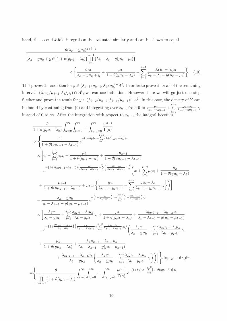
hand, the second k-fold integral can be evaluated similarly and can be shown to equal

θ(λk − yµk)a+k−1

(λk − yµk + y)a{1 + θ(yµk − λk)}k−1∏

i=1{λk − λi − y(µk − µi)}

×

{

aλk

λk − yµk + y+

µk

1 + θ(yµk − λk)+

k−1∑

i=1

λkµi − λiµk

λk − λi − y(µk − µi)

}

. (10)

This proves the assertion for y ∈ (λk−1/µk−1, λk/µk)∩A∁ . In order to prove it for all of the remaining

intervals (λj−1/µj−1, λj/µj) ∩ A∁, we can use induction. Howewer, here we will go just one step

further and prove the result for y ∈ (λk−2/µk−2, λk−1/µk−1)∩A∁. In this case, the density of Y can

be found by continuing from (9) and integrating over zk−1 from 0 to ywλk−1−yµk−1

+k−2∑

i=1

yµi−λi

λk−1−yµk−1

zi

instead of 0 to ∞. After the integration with respect to zk−1, the integral becomes

θ


∫ ∞

w=0

∫ ∞

z1=0· · ·

∫ ∞

zk−2=0

wa−1

Γ(a)

×

{

1

1 + θ(yµk−1 − λk−1)e−(1+θy)w−

k−2∑

i=1


×

[

w +k−2∑

i=1µizi +

µk

1 + θ(yµk − λk)+

µk−1

1 + θ(yµk−1 − λk−1)

− e−{1+θ(yµk−1−λk−1)}

(

ywλk−1

−yµk−1

+k−2∑

i=1

yµi−λiλk−1

−yµk−1

zi

)

(

w +k−2∑

i=1µizi +

µk


+µk−1

1 + θ(yµk−1 − λk−1)+ µk−1

{

yw

λk−1 − yµk−1+

k−2∑

i=1

yµi − λi

λk−1 − yµk−1zi

})]

−λk − yµk

λk − λk−1 − y(µk − µk−1)e−(

1+ y

λk−yµk

)

w−k−2∑

i=1

(


)

zi

×

[

λkw

λk − yµk+

k−2∑

i=1

λkµi − λiµk

λk − yµkzi +

µk

1 + θ(yµk − λk)+

λkµk−1 − λk−1µk

λk − λk−1 − y(µk − µk−1)

− e−(

1+yµk−1

−λk−1

λk−yµk

)(

yw

λk−1−yµk−1

+k−2∑

i=1

yµi−λiλk−1

−yµk−1

zi

)

(

λkw

λk − yµk+

k−2∑

i=1

λkµi − λiµk

λk − yµkzi

+µk

1 + θ(yµk − λk)+

λkµk−1 − λk−1µk

λk − λk−1 − y(µk − µk−1)

+λkµk−1 − λk−1µk

λk − yµk

{

λkw

λk − yµk+

k−2∑

i=1

λkµi − λiµk

λk − yµkzi

})]

}


=

{

θk∏

i=k−1

{1 + θ(yµi − λi)

∫ ∞

w=0

∫ ∞

z1=0· · ·

∫ ∞

zk−2=0

wa−1


k−2∑

i=1


19

×

(

w +k−2∑

i=1µizi +

µk−1

1 + θ(yµk−1 − λk−1)+

µk


)


}

−

{

θ(λk − yµk)

{1 + θ(yµk − λk)}{λk − λk−1 − y(µk − µk−1)}

∫ ∞

w=0

∫ ∞

z1=0· · ·

∫ ∞

zk−2=0

wa−1

Γ(a)

× e−(

1+ y

λk−yµk

)

w−k−2∑

i=1

(


)

zi

(

λkw

λk − yµk+

k−2∑

i=1

λkµi − λiµk

λk − yµkzi

+λkµk−1 − λk−1µk

λk − λk−1 − y(µk − µk−1)+

µk


)


}

−

{

θ


∫ ∞

w=0

∫ ∞

z1=0· · ·

∫ ∞

zk−2=0

wa−1

Γ(a)e−(

1+ y

λk−1−yµk−1

)

w−k−2∑

i=1

(

1+yµi−λi

λk−1−yµk−1

)

zi

×

[

1

1 + θ(yµk−1 − λk−1)

(

w +k−2∑

i=1µizi +

µk−1

1 + θ(yµk−1 − λk−1)+

µk


)

−λk − yµk

λk − λk−1 − y(µk − µk−1)

(

λk−1w

λk−1 − yµk−1+

k−2∑

i=1

λk−1µi − λiµk−1

λk−1 − yµk−1zi

+λk−1µk − λkµk−1

λk−1 − λk − y(µk−1 − µk)+

µk


)]


}

. (11)

Here, it can be seen that after performing all necessary integrations, the terms in the first two

braces reduce to (8) and (10), respectively. On the other hand, by using the facts that

1

1 + θ(yµk−1 − λk−1)−

λk − yµk

λk − λk−1 − y(µk − µk−1)

={1 + θ(yµk − λk)}(λk−1 − yµk−1)

{1 + θ(yµk−1 − λk−1)}{λk−1 − λk − y(µk−1 − µk)}

and

1

1 + θ(yµk−1 − λk−1)

(

µk−1

1 + θ(yµk−1 − λk−1)+

µk


)

−λk − yµk

λk − λk−1 − y(µk − µk−1)

(

λk−1µk − λkµk−1

λk−1 − λk − y(µk−1 − µk)+

µk


)

={1 + θ(yµk − λk)}(λk−1 − yµk−1)

{1 + θ(yµk−1 − λk−1)}{λk−1 − λk − y(µk−1 − µk)}

×

(

λk−1µk − λkµk−1

λk−1 − λk − y(µk−1 − µk)+

µk−1

1 + θ(yµk−1 − λk−1)

)

we obtain from (11), after carrying out all the integrations,

θ(λk−1 − yµk−1)a+k−1

(λk−1 − yµk−1 + y)a{1 + θ(yµk−1 − λk−1)}k∏

i=1i6=k−1

{λk−1 − λi − y(µk−1 − µi)}

×

{

aλk−1

λk−1 − yµk−1 + y+

µk−1

1 + θ(yµk−1 − λk−1)+

k∑

i=1i6=k−1

λk−1µi − λiµk−1

λk−1 − λi − y(µk−1 − µi)

}

20

and this establishes the result for ℓ = 1.

In order to prove it for ℓ > 1, set U =∑ℓ

i=1 Ui/θi so that we have

Y =U +

∑ki=1 λiZi

∑ki=1 µiZi + W

.

By solving for U , we get U = WY +∑k

i=1(Y µi − λi)Zi and dU/dY = W +∑k

i=1 µiZi, and upon

using Lemma 1, we conclude that the joint pdf of Y , Z’s, and W is

h(ℓ)(y,w, z1, . . . , zk;θ,λ,µ, a)

=

ℓ∑

j=1

( ℓ∏

i=1i6=j

θi

θi − θj

){

θjwa−1

Γ(a)

(

w +k∑

i=1µizi

)

e−(1+yθj )w−∑k

i=1{1+θj(yµi−λi)zi

}

,

w, z1, . . . , zk, wy +k∑

i=1(yµi − λi)zi > 0.

Now, in order to integrate out z’s and w, we have to work with terms within each brace separately.

However, all these quantities have the form of (6), and this yields the result.

Remark 1. The distribution presented in Theorem 2 as well as those derived in Theorems 3 and 4

below may possibly be deduced by the work of Provost and Rudiuk (1994). These authors discussed

the distribution of the ratio of dependent linear combinations of chi-square random variables (which

are in fact exponential random variables when the degrees of freedom equal two) via inverse Mellin

transforms. However, in our special case, we have chosen to derive the required distributions in a

straightforward manner through standard transformations of random variables rather than to try

to invert the corresponding Mellin transforms which are expressed as infinite power series.

Theorem 3. Let Z1, . . . , Zk,W be independent random variables, Z’siid∼ E(1) and W ∼ G(a, 1),

a > 0. Further, let λ = (λ1, · · · , λk) and µ = (µ1, · · · , µk) be vectors of positive numbers such that

λi/µi is strictly increasing in i. Then, the pdf of the random variable

Y =

∑ki=1 λiZi

∑ki=1 µiZi + W

(12)

is

f(0,k)T (y;λ,µ, a) =

k∑

j=1

(λj − yµj)a+k−2

(λj − yµj + y)ak∏

i=1i6=j

{λj − λi − y(µj − µi)}

×

{

aλj

λj − yµj + y+

k∑

i=1i6=j

λjµi − λiµj

λj − λi − y(µj − µi)

}

I(0,

λj

µj

](y). (13)

21

Proof. From (12), we get Zk =k−1∑

i=1

Y µi−λi

λk−Y µkZi+

Y Wλk−Y µk

with dZk/dY =k−1∑

i=1

λkµi−λiµk

(λk−Y µk)2Zi+

Wλk

(λk−Y µk)2,

and so the joint pdf of Z1, . . . , Zk−1,W, Y is

h(y,w, z1, . . . , zk−1;λ,µ, a)

=wa−1

Γ(a)(λk − yµk)2

{

wλk +k−1∑

i=1(λkµi − λiµk)zi

}

e−(

1+ y

λk−yµk

)

w−k−1∑

i=1

(


)

zi

,

w, z1, . . . , zk−1,wy

λk − yµk+

k−1∑

i=1

yµi − λi

λk − yµkzi > 0.

From the last inequality, we conclude that if y > λk/µk then the above joint pdf equals zero. Now,

working as in the proof of Theorem 2, one has to consider here the cases y ∈ (λk−1/µk−1, λk/µk),

(λk−2/µk−2, λk−1/µk−1), . . . , (0, λ1/µ1) and carry out the integrations to arrive at the required

result.

Remark 2. Let U ∼ E(1) independently of Z’s and W . Then, by Theorem 2, for any θ > 0,

Y ′θ =

U/θ +∑k

i=1 λiZi∑k

i=1 µiZi + W∼ f

(1,k)T (y; θ,λ,µ, a).

We have limθ→∞ Y ′θ = Y almost surely and consequently in distribution as well. On the other hand,

it can be verified that limθ→∞ f(1,k)T (y; θ,λ,µ, a) = f

(0,k)T (y;λ,µ, a) for all y > 0. Hence, Theorem 3

could be deduced from Theorem 2 by using a limiting argument provided some additional regularity

conditions would be satisfied. But, direct transformation of variables is sufficient for proving the

result.

Theorem 4. Let U1, . . . , Uℓ, Z1, . . . , Zkiid∼ E(1), and θ = (θ1, · · · , θℓ), λ = (λ1, · · · , λk) and

µ = (µ1, · · · , µk) be vectors of positive numbers such that all θ’s are distinct and λi/µi is strictly

increasing in i. Then,

Y =

∑ℓi=1 Ui/θi +

∑ki=1 λiZi

∑ki=1 µiZi

∼ f(ℓ,k)T (y;θ,λ,µ, 0).

Proof. The proof proceeds exactly as that of Theorem 2, and everything works in the same way

except that there is no integral here with respect to w.

Theorem 5. Let U1, . . . , Uℓ,W be independent random variables, U ’siid∼ E(1) and W ∼ G(a, 1),

a > 0. Further, let θ = (θ1, . . . , θℓ) be a vector of distinct positive numbers. Then, the pdf of the

random variable

Y =

∑ℓi=1 Ui/θi

W

is

f(ℓ,0)T (y;θ, a) =

ℓ∑

j=1

( ℓ∏

i=1i6=j

θi

θi − θj

)

aθj

(1 + yθj)a+1, y > 0.

22

Proof. Using Lemma 1, it can be shown rather easily.

Theorem 6. Let U,Z,W be independent random variables, U,Ziid∼ E(1) and W ∼ G(a, 1), a > 0.

Also, let c > 0. Then, the pdf of the random variable

Y =c(U − Z)

U + Z + W

is given by

gT (y; c, a) =a + 1

2c

(

1 −|y|

c

)a

I(−c,c)(y).

Proof. Since c is just a scale parameter, consider first c = 1 and set R = U −Z, S = U + Z. Then,

U = (S + R)/2, Z = (S − R)/2, with Jacobian 1/2 and so the joint density of R,S,W is

gR,S,W (r, s, w) =wa−1

2Γ(a)e−s−w, w > 0, s + r > 0, s − r > 0.

Since Y = R/(S + W ), we have R = Y (S + W ), dR/dY = S + W , and the joint density of Y, S,W

is

gT,S,W (y, s, w) =wa−1

2Γ(a)e−s−w, w > 0, (1 + y)s + yw > 0, (1 − y)s − yw > 0.

But

{(y, s, w) : w > 0,(1 + y)s + yw > 0, (1 − y)s − yw > 0}

={(y, s, w) : w > 0,−1 < y < 0, s > −yw/(1 + y)}∪

{(y, s, w) : w > 0, 0 6 y < 1, s > yw/(1 − y)}

and so,

gT (y; c = 1, a) =

∫ ∞w=0

∫ ∞s=−yw/(1+y)

wa−1

2Γ(a) e−s−wdsdw, −1 < y < 0,∫ ∞w=0

∫ ∞s=yw/(1−y)

wa−1

2Γ(a) e−s−wdsdw, 0 6 y < 1

=a + 1

2(1 − |y|)aI(−1,1)(y).

References

Arnold, B.C., Balakrishnan, N. and Nagaraja, H.N. (2008). A First Course in Order Statistics, ClassicEdition, SIAM, Philadelphia.

Bain, L.J. and Engelhardt, M. (1973). Interval estimation for the two-parameter double exponential dis-tribution, Technometrics, 15, 875–887.

Balakrishnan, N. (2007). Progressive censoring methodology: An appraisal (with discussions), Test, 16,211-296.

23

Balakrishnan, N. and Cutler, C.D. (1995). Maximum likelihood estimation of Laplace parameters basedon Type-II censored samples, In Statistical Theory and Applications: Papers in Honor of Herbert A.

David (Eds., H.N. Nagaraja, P.K. Sen and D.F. Morrison), pp. 145–151, Springer-Verlag, New York.

Chernoff, H., Gastwirth, J.L. and Johns, M.V. (1967). Asympotic distribution of linear combinations offunctions of order statistics with applications to estimation, The Annals of Mathematical Statistics,38, 52–72.

Childs, A. and Balakrishnan, N. (1996). Conditional inference procedures for the Laplace distributionbased on type-II right censored samples, Statistics & Probability Letters, 31, 31–39.

Childs, A. and Balakrishnan, N. (1997). Maximum likelihood estimation of Laplace parameters based ongeneral Type-II censored samples, Statistical Papers, 38, 343–349.

David, H.A. and Nagaraja, H.N. (2003). Order Statistics, Third Edition, John Wiley & Sons, Hoboken,New Jersey.

Efron, B. and Tibshirani, R. (1993). An Introduction to the Bootstrap, Chapman & Hall, New York.

Grice, J.V., Bain, L.J. and Engelhardt, M. (1978). Comparison of conditional and unconditional confi-dence intervals for the double exponential distribution, Communications in Statistics – Simulation

and Computation, 7, 515–524.

Iliopoulos, G. and Balakrishnan, N. (2009). Conditional independence of blocked ordered data, Statistics

& Probability Letters, 79, 1008–1015.

Johnson, N.L., Kotz, S. and Balakrishnan, N. (1995). Continuous Univariate Distributions, Vol. 2, Secondedition, John Wiley & Sons, New York.

Kappenman, R.F. (1975). Conditional confidence intervals for double exponential distribution parameters,Technometrics, 17, 233–235.

Kotz, S., Kozubowski, T.J. and Podgorski, K. (2001). The Laplace Distribution and Generalizations,Birkhauser, Boston.

Provost, S.B. and Rudiuk, E.M. (1994). The exact density function of the ratio of two dependent linearcombinations of chi-square variables, Annals of the Institute of Statistical Mathematics, 46, 557–571.

Sansing, R.C. (1976). The t-statistic for a double exponential distribution, SIAM Journal on Applied

Mathematics, 31, 634–645.

24

n 90% 95% 99% n 90% 95% 99%15 84.8% 91.6% 98.4% 40 86.7% 92.5% 98.1%20 85.9% 92.2% 98.3% 45 86.5% 92.3% 98.0%25 85.6% 91.8% 98.0% 50 86.9% 92.7% 98.1%30 86.4% 92.3% 98.1% 55 86.8% 92.5% 98.0%35 86.1% 92.1% 98.0% 60 87.1% 92.8% 98.1%

Table 1: Exact coverage probabilities of confidence intervals for µ in the case of complete samplesbased on the normal approximation proposed by Bain and Engelhardt (1973).

n 90% 95% 99% n 90% 95% 99%15 87.6% 93.0% 98.3% 40 89.6% 94.9% 98.9%20 87.8% 93.6% 98.6% 45 89.4% 94.7% 99.1%25 88.3% 93.8% 98.7% 50 89.9% 95.0% 99.0%30 88.6% 94.4% 99.0% 55 90.0% 95.1% 99.0%35 88.9% 94.4% 98.8% 60 89.1% 94.7% 99.0%

Table 2: Estimated coverage probabilities of bootstrap confidence intervals for µ in the case ofcomplete samples based on 10000 simulations and 1000 bootstrap samples.

n 90% 95% 99% n 90% 95% 99%15 89.5% 94.3% 98.0% 40 90.5% 94.8% 98.6%20 89.8% 94.4% 98.3% 45 90.3% 94.9% 98.6%25 89.3% 94.5% 98.5% 50 89.8% 94.6% 98.6%30 90.3% 94.9% 98.6% 55 90.4% 95.0% 98.5%35 90.4% 95.0% 98.8% 60 90.2% 94.7% 98.7%

Table 3: Estimated coverage probabilities of bootstrap confidence intervals for σ in the case ofcomplete samples based on 10000 simulations and 1000 bootstrap samples.

25

n 0.1 0.05 0.025 0.01 0.0052 2.5 5 10 25 503 1.6646 2.4271 3.3166 5.0990 7.14144 1.0548 1.5024 2.0000 2.7583 3.44565 .9418 1.3144 1.6841 2.1910 2.61216 .7532 1.0366 1.3226 1.7135 2.02527 .7068 .9702 1.2237 1.5524 1.80308 .6093 .8287 1.0421 1.3214 1.53439 .5843 .7949 .9945 1.2483 1.4364

10 .5226 .7061 .8812 1.1058 1.273011 .5070 .6856 .8536 1.0647 1.219212 .4635 .6234 .7744 .9656 1.106213 .4529 .6098 .7564 .9396 1.072514 .4201 .5631 .6973 .8656 .988315 .4125 .5535 .6847 .8478 .965516 .3865 .5168 .6383 .7898 .899717 .3808 .5096 .6290 .7769 .883418 .3597 .4799 .5914 .7300 .830119 .3552 .4743 .5844 .7203 .817820 .3375 .4495 .5531 .6813 .773621 .3340 .4451 .5476 .6737 .764122 .3189 .4241 .5210 .6407 .726623 .3160 .4205 .5166 .6347 .719024 .3030 .4023 .4937 .6062 .686725 .3006 .3994 .4900 .6013 .680626 .2892 .3835 .4701 .5764 .652427 .2871 .3810 .4670 .5724 .647428 .2770 .3670 .4494 .5504 .622529 .2752 .3648 .4468 .5470 .618330 .2662 .3523 .4311 .5275 .596231 .2647 .3505 .4289 .5246 .592632 .2566 .3392 .4148 .5071 .572733 .2552 .3377 .4128 .5045 .569634 .2478 .3275 .4001 .4887 .551735 .2467 .3261 .3984 .4865 .549036 .2399 .3168 .3868 .4721 .532637 .2389 .3156 .3853 .4702 .530338 .2327 .3070 .3747 .4570 .515439 .2318 .3060 .3733 .4553 .513340 .2261 .2981 .3636 .4432 .5000

Table 4: Upper quantiles of T = (µ − µ)/σ in the case of complete samples. By symmetry, thecorresponding lower quantiles are their negatives.

26

n 0.995 0.99 0.975 0.95 0.9 0.1 0.05 0.025 0.01 0.0052 0.0050 0.0100 0.0250 0.0501 0.1006 1.6359 2.0565 2.4659 2.9951 3.38873 0.0473 0.0672 0.1073 0.1541 0.2246 1.4088 1.6976 1.9763 2.3345 2.60004 0.1103 0.1408 0.1962 0.2553 0.3383 1.5006 1.7616 2.0093 2.3228 2.55225 0.1591 0.1930 0.2521 0.3124 0.3941 1.4188 1.6374 1.8433 2.1022 2.29086 0.2087 0.2459 0.3091 0.3720 0.4554 1.4333 1.6345 1.8228 2.0582 2.22887 0.2448 0.2827 0.3459 0.4079 0.4887 1.3884 1.5684 1.7359 1.9444 2.09508 0.2818 0.3209 0.3852 0.4474 0.5276 1.3883 1.5567 1.7129 1.9066 2.04609 0.3092 0.3482 0.4117 0.4726 0.5503 1.3590 1.5144 1.6579 1.8354 1.9628

10 0.3378 0.3771 0.4406 0.5010 0.5776 1.3551 1.5023 1.6379 1.8050 1.924811 0.3595 0.3984 0.4609 0.5200 0.5944 1.3342 1.4723 1.5993 1.7554 1.867112 0.3824 0.4112 0.4833 0.5416 0.6147 1.3294 1.4613 1.5824 1.7309 1.836913 0.4000 0.4384 0.4995 0.5565 0.6278 1.3134 1.4387 1.5534 1.6939 1.794114 0.4188 0.4570 0.5174 0.5737 0.6437 1.3086 1.4290 1.5391 1.6737 1.769515 0.4336 0.4713 0.5307 0.5859 0.6542 1.2959 1.4112 1.5164 1.6449 1.736216 0.4494 0.4867 0.5455 0.5999 0.6671 1.2914 1.4027 1.5041 1.6279 1.715717 0.4620 0.4989 0.5567 0.6100 0.6758 1.2810 1.3882 1.4858 1.6046 1.688918 0.4755 0.5120 0.5692 0.6218 0.6845 1.2767 1.3807 1.4752 1.5901 1.671619 0.4864 0.5224 0.5787 0.6304 0.6938 1.2681 1.3686 1.4599 1.5708 1.649420 0.4981 0.5338 0.5894 0.6404 0.7029 1.2642 1.3619 1.4506 1.5583 1.634521 0.5076 0.5429 0.5977 0.6479 0.7092 1.2567 1.3517 1.4377 1.5420 1.615722 0.5179 0.5528 0.6071 0.6565 0.7170 1.2532 1.3457 1.4295 1.5310 1.602723 0.5264 0.5609 0.6144 0.6631 0.7225 1.2467 1.3368 1.4183 1.5170 1.586724 0.5355 0.5697 0.6226 0.6707 0.7293 1.2434 1.3315 1.4110 1.5073 1.575225 0.5431 0.5769 0.6291 0.6765 0.7342 1.2378 1.3237 1.4013 1.4951 1.561226 0.5513 0.5867 0.6364 0.6832 0.7401 1.2348 1.3189 1.3947 1.4865 1.551127 0.5581 0.5912 0.6422 0.6884 0.7445 1.2298 1.3120 1.3861 1.4757 1.538828 0.5655 0.5983 0.6487 0.6944 0.7498 1.2270 1.3076 1.3802 1.4679 1.529629 0.5717 0.6041 0.6540 0.6991 0.7537 1.2225 1.3015 1.3726 1.4584 1.518730 0.5784 0.6105 0.6599 0.7045 0.7584 1.2199 1.2974 1.3672 1.4513 1.510531 0.5841 0.6159 0.6647 0.7088 0.7620 1.2159 1.2919 1.3603 1.4427 1.500732 0.5902 0.6217 0.6701 0.7136 0.7663 1.2135 1.2882 1.3554 1.4363 1.493233 0.5955 0.6266 0.6745 0.7175 0.7695 1.2099 1.2832 1.3492 1.4286 1.484434 0.6011 0.6320 0.6793 0.7220 0.7734 1.2076 1.2798 1.3447 1.4227 1.477535 0.6059 0.6365 0.6834 0.7256 0.7764 1.2043 1.2753 1.3390 1.4157 1.469536 0.6111 0.6414 0.6879 0.7297 0.7799 1.2022 1.2721 1.3348 1.4103 1.463237 0.6155 0.6456 0.6916 0.7329 0.7826 1.1991 1.2679 1.3297 1.4039 1.455938 0.6203 0.6502 0.6958 0.7367 0.7859 1.1972 1.2650 1.3258 1.3989 1.450139 0.6243 0.6541 0.6992 0.7398 0.7884 1.1944 1.2612 1.3210 1.3930 1.443340 0.6290 0.6583 0.7031 0.7432 0.7914 1.1925 1.2584 1.3175 1.3883 1.4380

Table 5: Quantiles of S = σ/σ in the case of complete samples.

1.96 1.96 3.60 3.80 4.79 5.66 5.76 5.78 6.27 6.30 6.767.65 7.84 7.99 8.51 9.18 10.13 10.24 10.25 10.43 11.45 11.48

11.75 11.81 12.34 12.78 13.06 13.29 13.98 14.18 14.40 16.22 17.06

Table 6: Data on differences in flood stages for two stations on the Fox River, Wisconsin, for 33different years.

27

exact likelihood inference for laplace distribution based ... · exact likelihood inference for...

Documents