exact methods for solving traveling salesman problems with ... · the traveling salesman problem...
TRANSCRIPT
Exact Methods for Solving Traveling Salesman Problems withPickup and Delivery in Real Time
Ryan J. O’Neil · Karla Hoffman
September 2, 2018
Abstract The Traveling Salesman Problem with Pickup
and Delivery (TSPPD) describes the problem of finding
a minimum cost path in which pickups precede their
associated deliveries. The TSPPD is particularly im-
portant in the growing field of Dynamic Pickup and
Delivery Problems (DPDP). These include the many-
to-many Dial-A-Ride Problems (DARP) of companies
such as Uber and Lyft, and meal delivery services pro-
vided by Grubhub. We examine exact methods for solv-
ing TSPPDs where orders from different pickup loca-
tions can be carried simultaneously in real-time appli-
cations, in which finding high quality solutions quickly
(often in less than a second) is often more important
that proving the optimality of such solutions. We con-
sider enumeration, Constraint Programming (CP), Mixed
Integer Programming (MIP), and hybrid methods com-
bining CP and MIP. Our CP formulations examine mul-
tiple techniques for ensuring pickup and delivery prece-
dence relationships. Finally, we attempt to provide guid-
ance about which of these methods may be most ap-
propriate for fast TSPPD solving given various time
budgets and problem sizes.
Keywords traveling salesman problem; pickup and
delivery; integer programming; constraint program-
Ryan J. O’NeilSystems Engineering & Operations Research DepartmentGeorge Mason University, Fairfax, Virginia 22030E-mail: [email protected] Engineering DepartmentGrubhub, Chicago, Illinois 60602E-mail: [email protected]
Karla HoffmanSystems Engineering & Operations Research DepartmentGeorge Mason University, Fairfax, Virginia 22030E-mail: [email protected]
ming; computational experiments; hybrid optimization
methods; real-time optimization
1 Introduction
The Traveling Salesman Problem (TSP) is the search
for a minimum cost Hamiltonian circuit connecting a
set of locations. In general, the TSP is NP-complete
[34]. The first paper of note related to TSP research
solved an instance of “49 cities, one in each of the 48
states and Washington, D.C.” [10]. Algorithms now ex-
ist that, given sufficient time, can solve TSPs with tens
of thousands of nodes, and its computational bound-
aries continue to be pushed forward [2].
The TSP is an important problem in inspiring algo-
rithmic research, to the substantial benefit of the op-
timization community. It also provides a practical ap-
plication in its own right, particularly in the context of
Vehicle Routing Problems (VRP). VRPs are common
in industry and involve routing a set of vehicles to visit
a set of nodes at minimum cost. At its surface, the only
substantive difference between the TSP and the VRP is
the latter’s use of multiple vehicles to service customer
demand.
The Pickup and Delivery Problem (PDP) is an in-
creasingly prevalent industrial form of the VRP in which
each of a set of requests must be picked up from one
or more locations and delivered to one or more delivery
points. Pickups must precede their associated deliveries
in any feasible route, and each pair must be serviced by
the same vehicle. Pickup and delivery locations can be
distinct to each request, as in the many-to-many Dial-
A-Ride Problem (DARP) of Psaraftis (1980) [37] Bert-
simas et al. (2018) [7] and the Meal Delivery Routing
Problem (MDRP). Given multiple pickup and delivery
2 Ryan J. O’Neil, Karla Hoffman
requests, the PDP seeks to route a set of vehicles to
service those requests at minimum cost [38].
Solving a PDP with a single vehicle is equivalent
to solving a TSP with precedence constraints on the
pickup and delivery nodes. This form is referred to as
the Traveling Salesman Problem with Pickup and De-
livery (TSPPD) [12]. There is a great deal of litera-
ture on the TSP and some of its variants, such as the
TSP with Time Windows (TSPTW) [2]. In contrast,
there has been less attention paid to the TSPPD, de-
spite its practical applicability [38]. TSPPDs and their
variants play an increasingly important role in indus-
trial routing applications. This importance is witnessed
by a proliferation of ride hailing and sharing companies,
as well as on-demand delivery service providers for ev-
erything from groceries, alcoholic beverages, and meals,
to snacks and convenience store items.
Different forms of on-demand pickup and delivery
have their own objectives, constraints, and levels of dy-
namism and urgency for decision making [28]. For in-
stance, in dynamic DARP, end users are inconvenienced
from the moment they request a ride. In the MDRP,
time from request to delivery cannot be less than the
restaurant preparation time and travel time from the
restaurant to the diner.
1.1 Problems with Small Routes
The divide between research and industrial use of the
TSP becomes clearly evident when one considers prac-
tical limitations associated with routing. For example,
delivery trucks are often limited to routes of fewer than
100 stops due to physical considerations, such as vehicle
capacity [9]. Routes used for high volume restaurant de-
livery are even shorter due to the perishability of goods,
and typically involve fewer than 10 stops.
Even in the context of the broader PDP with many
vehicles and many more nodes (e.g. hundreds or thou-
sands), the allowable individual routes tend to be rela-
tively short. Solving real-world delivery problems often
requires solving, in a very short time frame (i.e. frac-
tions of a second to not more than minutes), a huge
numbers of problems each having a very small number
of nodes. And, often, resolving some subset of these
problems as the delivery service learns of changing de-
mand and/or service times.
This lack of attention reflects a common theme of
exact approaches in the TSP optimization literature,
which seek to optimize ever longer routes. The pri-
mary mechanism for finding exact solutions to TSPs
is a branch-and-cut procedure based on Dantzig et al.
(1954) [10] in which the TSP is relaxed into a two-
matching problem, binary arc variables are relaxed to
continuous variables with 0-1 bounds, and cuts are added
to the formulation as infeasible solutions are found by
the optimization. Thus the procedure begins with an
infeasible solution and works toward feasibility. The
bulk of the computation is based on getting good lower
bounds on the problem, as good upper bounds are usu-
ally obtained through the Lin-Kernighan heuristic.
Branch-and-cut is by no means the only model for
solving TSPs. One could consider adding cuts to the
two-matching or assignment relaxations as pure inte-
ger solutions are found, as done in Pferschy and Stanek
(2016) [36]. This approach may not be as effective in
proving optimality, but it removes complexity and cut-
ting planes, making its implementation more conve-
nient. Such approaches retain the issue of starting in-
feasible and working toward feasibility. In either case,
most procedures employ heuristics to obtain feasible so-
lutions, thereby supplying upper bounds on the prob-
lem.
Infeasibility can be particularly painful in dynamic
real-time logistics, where optimization procedures are
time limited. Such problems may prefer obtaining a
“good” solution quickly to an optimal solution even-
tually. In these circumstances, one might reasonably
ask, “What is the cost of optimality?” Or the corol-
lary, “What is the value of knowing one is likely to
obtain a near-optimal solution within a certain amount
of time?” For the class of problems that we are consid-
ering, time budgets for route optimization are on the
order of milliseconds or, at most, seconds.
1.2 Hybrid Methods
Another issue with standard exact approaches to solv-
ing practical TSP instances is inflexibility. Industrial
problems often have side constraints. Of particular in-
terest here, the PDP requires that associated pickups
and deliveries be serviced by the same vehicle and that
the former precede the latter.
Other common constraints involve time windows,
such as in the PDPTW [11]. For example, for meal de-
livery service operations, an order cannot be picked up
from a restaurant before it is ready. A delivery can-
not be made to a residence outside of an agreed-upon
time window. Further, vehicles may have capacity con-
straints. This requirement is particularly important if
bicycle couriers are used, as they have limited carrying
capacity. These are just a few of the potential side con-
straints that may be required in an industrial model for
either physical or business reasons.
Milano et al. (2001) [30] characterize the strengths
and weaknesses of Mixed Integer Programming (MIP)
Exact Methods for Solving TSPPDs in Real Time 3
and Constraint Programming (CP) in terms of opti-
mality and feasibility reasoning. MIP excels at proving
optimality by working to improve both the upper and
the lower bounds, but may take longer to obtain a fea-
sible solution. The slowness in finding a first feasible
solution is often because algebraic (linear) formulations
fail to encode the special structure of a problem with-
out requiring the use of “big M’s” to indicate either-or
syntax. Thus, side constraints such as precedence con-
straints or time windows that occur in TSP related to
vehicle routing can be challenging for a MIP solver, but
they adapt quite naturally to CP, since CP solvers can
handle them directly in their propagation and search
strategies [9, 35].
On the other hand, CP is much less efficient at op-
timality reasoning than MIP. This is partly due to poor
propagation on objective functions, and partly due to
a lack of built-in concepts around dual bounds and
reduced-cost variable fixing. We address these difficul-
ties by studying both MIP and CP forms of the TSPPD,
then integrating them into hybrid models that combine
the benefits of the two, similar to the models proposed
in Focacci et al. (1999) [17] and Focacci et al. (2002)
[16].
We test these models using problem instances gener-
ated from real-world meal delivery data. These are built
from actual pickup and delivery locations observed at
Grubhub, along with expected travel times connecting
location pairs. We use a variety of problem sizes to char-
acterize the performance of enumerative, MIP, CP, and
hybrid models, and attempt to provide advice regard-
ing which techniques are most appropriate for real-time
optimization given varying time budgets and problem
sizes.
Contributions of this paper include extensive com-
putational experiments using these models for solving
TSPPD instances, along with guidance for which tech-
niques work best quickly and how they can be hybridized
effectively. Our test set and source code for all model
implementations are available for continued experimen-
tation [20, 32]. Further, in the CP model implemen-
tation, we compare different forms of precedence that
operate on circuit constraints, and provide a complete
description of a propagator that enforces precedence
without the use of time windows. Finally, we explore
different branching forms for CP applied to the TSPPD.
2 Background
The Traveling Salesman Problem with Pickup and De-
livery (TSPPD) is a modification of the Traveling Sales-
man Problem (TSP) that includes side constraints en-
+0
+i
+j
-i
-j
-0
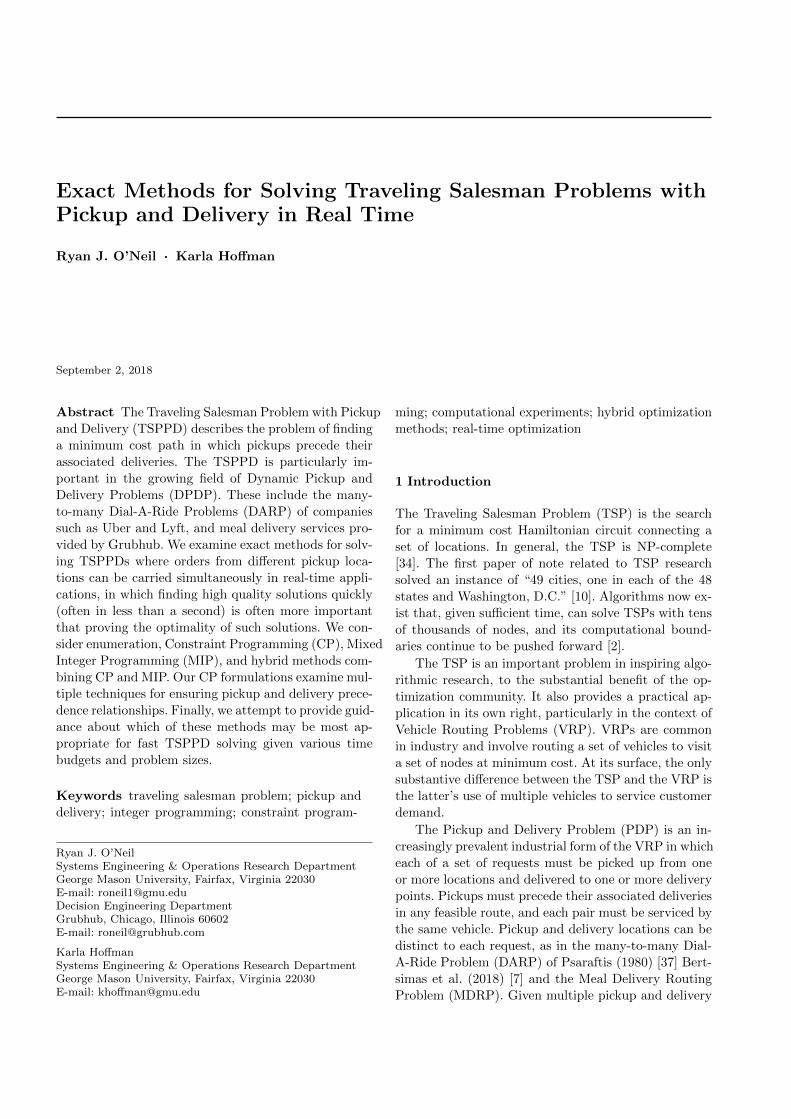
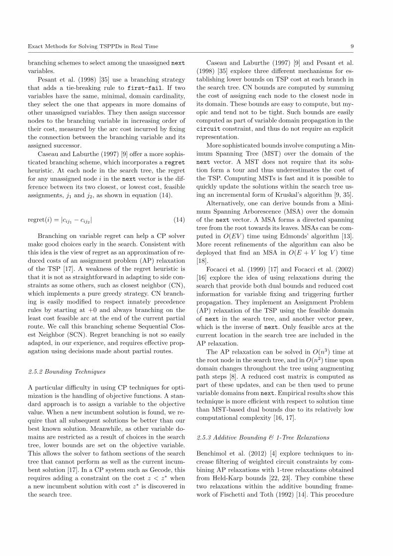
Fig. 1 Example TSPPD graph structure.
forcing precedence among pickup and delivery node pairs.
Each of n requests has a pickup node and a delivery
node, and its pickup must occur before its delivery for
a route to be feasible. The objective of the problem is
to minimize total distance traveled while visiting each
node exactly once. The TSPPD is formally described
in Ruland and Rodin (1997) [38] and Dumitrescu et al.
(2010) [12].
2.1 The TSPPD Polytope
The TSPPD is defined on an ordered set of pickup
nodes V+ = {+1, . . . ,+n} and associated delivery nodes
V− = {−1, . . . ,−n} such that (+i,−i) form a request
and +i must precede −i in a feasible route. V is de-
fined as the union of V+ and V− with the addition of
origin and destination nodes {+0,−0}. E± is the set of
edges connecting V+∪V−. E is the union of E± with all
feasible edges connecting to the origin and destination
nodes. The graph G = (V,E) includes all nodes and
edges required to describe the TSPPD.
V = {+0,−0} ∪ V+ ∪ V−E = {(+0,−0)} ∪ {(+0,+i) | i ∈ V+}∪ {(−0,−i) | i ∈ V−} ∪ E±For modeling convenience, the edge (+0,−0) must
be included in any feasible solution. The set of edges
E is defined such that it includes only feasible edges.
That is, it is not possible that a TSPPD route begins
with a delivery or ends with a pickup. Figure 1 shows
an example of the feasible edges for a TSPPD with
two requests. Note that it is possible to use the same
formulation to solve Hamiltonian paths with precedence
rather than circuits by simply assigning a cost of zero
to the (+0,−0) edge.
2.1.1 The Symmetric TSPPD
In the case of the symmetric TSPPD (STSPPD), each
edge (i, j) ∈ E is the same as the edge (j, i) and has
4 Ryan J. O’Neil, Karla Hoffman
the same costs and edge variables. cij specifies a non-
negative cost for each edge (i, j) ∈ E. By convention,
c+0,−0 = 0. xij ∈ {0, 1} is a binary decision variable for
each (i, j) ∈ E with the value xij = 1 if the edge (i, j)
is in a solution and 0 otherwise. δ(S) = {(i, j) ∈ E | i ∈S, j /∈ S} is the cutset containing edges that connect
S ⊂ V and S ⊂ V . For any node i ∈ V , δ(i) = δ({i}).The STSPPD is defined using Formulation 1, as in Ru-
land and Rodin (1997) [38].
min∑
(i,j)∈E
cijxij
s.t. x+0,−0 = 1 (1)
x(δ(i)) = 2 ∀ i ∈ V (2)
x(δ(S)) ≥ 2 ∀ S ⊂ V (3)
x(δ(S)) ≥ 4 ∀ S ⊂ V, {+0,−i} ⊂ S,{−0,+i} ⊂ V \ S (4)
xij ∈ {0, 1} ∀ (i, j) ∈ A
Formulation 1: STSPPD as provided by Ruland and Rodin [38]
Constraint (1) requires that the edge connecting the
origin and destination nodes be part of any feasible
solution. The degree constraints (2) require that each
node is entered and exited in all feasible routes, but by
itself leaves open the possibility of disconnected sub-
tours. Constraints (3) accomplish subtour elimination,
forming a complete representation of the TSP. The fi-
nal set of constraints (4) require that pickups occur in
routes before their respective deliveries [38].
2.1.2 The Asymmetric TSPPD
The asymmetric TSP (ASTP) polytope can be similarly
adapted to the asymmetric TSPPD (ATSPPD) by as-
sociating the x variables with arcs (i.e. directed edges)
and replacing the two-degree constraints with assign-
ment constraints. Instead of an edge set E we define an
arc set A which contains only the feasible arcs for the
ATSPPD.
A = {(−0,+0)}∪ {(+0,+i) | + i ∈ V+}∪ {(−i,−0) | − i ∈ V−}∪ {(+i, j) | + i ∈ V+, j ∈ (V+ ∪ V−) \ {+i}}∪ {(−i, j) | − i ∈ V+, j ∈ (V+ ∪ V−) \ {+i,−i}}
Formulation 2 is more general since it supports arc
costs that are not the same bidirectionally. Further, it is
intuitively satisfying to consider the TSPPD this way,
as there is a natural asymmetry built into the structure
of the problem: pickups must precede their associated
deliveries. As in Formulation 1, the x−0,+0 arc connect-
ing the start and end nodes must be part of any feasible
tour, +0 must connect to a pickup, and −0 must be
preceded by a delivery. One small additional difference
is that Formulation 2 does not include x variables for
arcs starting at a delivery and ending at its associated
pickup.
min∑
(i,j)∈A
cijxij
s.t.∑
(i,j)∈A
xij = 1 ∀ i ∈ V (5)
∑(i,j)∈A
xij = 1 ∀ j ∈ V (6)
x(δ(S)) ≥ 1 ∀ S ⊂ V (7)
x(δ(S)) ≥ 4 ∀ S ⊂ V, {+0,−i} ⊂ S,{−0,+i} ⊂ V \ S
xij ∈ {0, 1} ∀ (i, j) ∈ A (8)
Formulation 2: ATSPPD
In Formulation 2, constraints (5) and (6) require
that each node directly precede and follow exactly one
other node. Constraints (7) accomplish subtour elim-
ination, while precedence is enforced using the same
constraints as in Formulation 1.
2.2 Enumerative Methods
One reason solving TSPs is challenging is that the num-
ber of feasible solutions grows as a factorial function of
the number of nodes. Yet enumeration may still be a
valid technique for solving small TSPPDs. If it is guided
by some information about the problem, enumeration
may be able to discover good routes quickly without
any overhead of model formulation.
In addition to more sophisticated models, we also
consider an enumerative approach. Our purpose is to
determine which size problems enumeration can suc-
cessfully solve, and at which point sophisticated mod-
eling techniques tend to more effectively solve the prob-
lem. Algorithm 1 uses a recursive function to search the
feasible set of TSPPD routes, while tracking the best
solution discovered at each point in the search tree.
This algorithm maintains a current node and a par-
tial tour starting at +0. Every recursion loops over the
arcs from the current node and appends each feasible
one to the tour individually prior to recursing. If an
arc’s added cost puts a partial route’s cost over that of
Exact Methods for Solving TSPPDs in Real Time 5
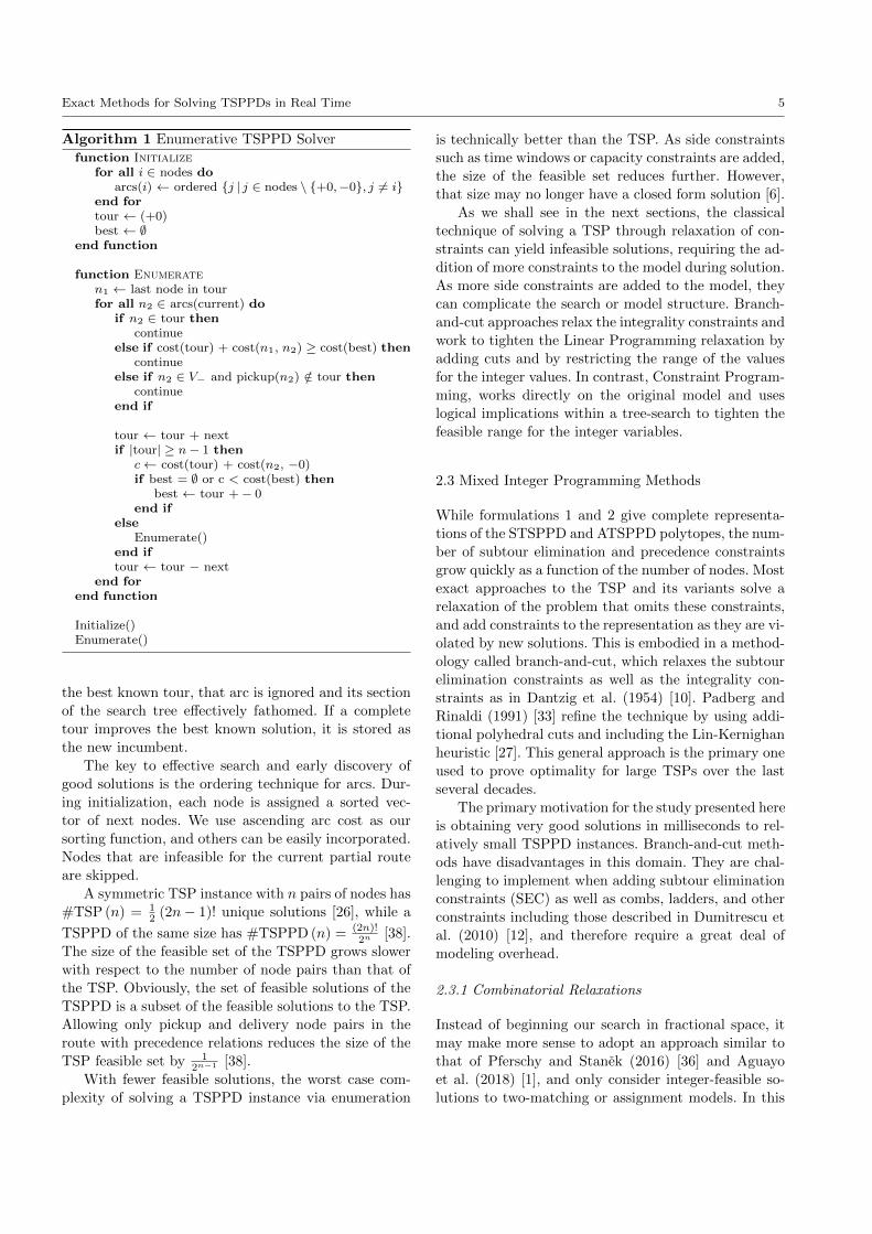
Algorithm 1 Enumerative TSPPD Solverfunction Initialize
for all i ∈ nodes doarcs(i) ← ordered {j | j ∈ nodes \ {+0,−0}, j 6= i}
end fortour ← (+0)best ← ∅
end function
function Enumeraten1 ← last node in tourfor all n2 ∈ arcs(current) do
if n2 ∈ tour thencontinue
else if cost(tour) + cost(n1, n2) ≥ cost(best) thencontinue
else if n2 ∈ V− and pickup(n2) /∈ tour thencontinue
end if
tour ← tour + nextif |tour| ≥ n− 1 then
c← cost(tour) + cost(n2, −0)if best = ∅ or c < cost(best) then
best ← tour +− 0end if
elseEnumerate()
end iftour ← tour − next
end forend function
Initialize()Enumerate()
the best known tour, that arc is ignored and its section
of the search tree effectively fathomed. If a complete
tour improves the best known solution, it is stored as
the new incumbent.
The key to effective search and early discovery of
good solutions is the ordering technique for arcs. Dur-
ing initialization, each node is assigned a sorted vec-
tor of next nodes. We use ascending arc cost as our
sorting function, and others can be easily incorporated.
Nodes that are infeasible for the current partial route
are skipped.
A symmetric TSP instance with n pairs of nodes has
#TSP (n) = 12 (2n− 1)! unique solutions [26], while a
TSPPD of the same size has #TSPPD (n) = (2n)!2n [38].
The size of the feasible set of the TSPPD grows slower
with respect to the number of node pairs than that of
the TSP. Obviously, the set of feasible solutions of the
TSPPD is a subset of the feasible solutions to the TSP.
Allowing only pickup and delivery node pairs in the
route with precedence relations reduces the size of the
TSP feasible set by 12n−1 [38].
With fewer feasible solutions, the worst case com-
plexity of solving a TSPPD instance via enumeration
is technically better than the TSP. As side constraints
such as time windows or capacity constraints are added,
the size of the feasible set reduces further. However,
that size may no longer have a closed form solution [6].
As we shall see in the next sections, the classical
technique of solving a TSP through relaxation of con-
straints can yield infeasible solutions, requiring the ad-
dition of more constraints to the model during solution.
As more side constraints are added to the model, they
can complicate the search or model structure. Branch-
and-cut approaches relax the integrality constraints and
work to tighten the Linear Programming relaxation by
adding cuts and by restricting the range of the values
for the integer values. In contrast, Constraint Program-
ming, works directly on the original model and uses
logical implications within a tree-search to tighten the
feasible range for the integer variables.
2.3 Mixed Integer Programming Methods
While formulations 1 and 2 give complete representa-
tions of the STSPPD and ATSPPD polytopes, the num-
ber of subtour elimination and precedence constraints
grow quickly as a function of the number of nodes. Most
exact approaches to the TSP and its variants solve a
relaxation of the problem that omits these constraints,
and add constraints to the representation as they are vi-
olated by new solutions. This is embodied in a method-
ology called branch-and-cut, which relaxes the subtour
elimination constraints as well as the integrality con-
straints as in Dantzig et al. (1954) [10]. Padberg and
Rinaldi (1991) [33] refine the technique by using addi-
tional polyhedral cuts and including the Lin-Kernighan
heuristic [27]. This general approach is the primary one
used to prove optimality for large TSPs over the last
several decades.
The primary motivation for the study presented here
is obtaining very good solutions in milliseconds to rel-
atively small TSPPD instances. Branch-and-cut meth-
ods have disadvantages in this domain. They are chal-
lenging to implement when adding subtour elimination
constraints (SEC) as well as combs, ladders, and other
constraints including those described in Dumitrescu et
al. (2010) [12], and therefore require a great deal of
modeling overhead.
2.3.1 Combinatorial Relaxations
Instead of beginning our search in fractional space, it
may make more sense to adopt an approach similar to
that of Pferschy and Stanek (2016) [36] and Aguayo
et al. (2018) [1], and only consider integer-feasible so-
lutions to two-matching or assignment models. In this
6 Ryan J. O’Neil, Karla Hoffman
approach we solve a combinatorial relaxation contain-
ing only the degree constraints. SEC are added within
the branch-and-bound search tree as they are violated.
Such constraints are implemented as “lazy” constraints
within the solver, which are allowed to cut off integer-
feasible solutions and are checked whenever a new can-
didate solution is found.
We take the same approach with the TSPPD: solve a
relaxation of the problem using only degree constraints
(2) for the STSPPD, or constraint sets (5) and (6)
for the ATSPPD. When a candidate solution is found,
check to see if it contains subtours or violates prece-
dence. If so, add SEC and precedence constraints as
appropriate. Once a tour covering all nodes and satis-
fying presence constraints is found, that tour is optimal.
As integer-feasible solutions are discovered in the
branch-and-bound tree, they are scanned for subtours.
T is the set containing all sets of nodes in a tour in
the current solution. If T > 1, then for each set of
nodes corresponding to a subtour S ∈ T , we add a lazy
constraint of either the form (3) or (7), eliminating that
subtour from future solutions.
Constraints (3) or (7) remove a given subtour from
the final solution. Thereafter, not all edges in the sub-
tour can exist in any new solution. An alternative and
equivalent formulation of the constraint is shown as (9)
below. We call constraints (3) and (7) the “cutset” form
and constraint (9) the “subtour” form, respectively.
∑i,j∈S
xij ≤ |S| − 1 (9)
The different SEC formulations achieve the same
end, but impact different sets of edges. In particular,
constraint set (9) includes not only the edges found in
a disconnected subtour, but all edges connecting the
nodes in the subtour S. This inclusion of additional
edges makes the constraint stronger, and follows from
the observation that only |S| − 1 edges from a subtour
can be in a Hamiltonian circuit, and that circuit is com-
prised of n edges, including (+0,−0) in the case of the
TSPPD. If only |S| − 1 edges from a subtour can be in
the final tour, there must be n− (|S| − 1) = n− |S|+ 1
edges that are not part of the subtour in the final solu-
tion.
Pferschy and Stanek (2016) [36] investigate the ben-
efits of switching between constraints (9) and (3), ob-
serving that the solution time for a MIP tends to in-
crease with the density of its constraint matrix. They
choose between the two formulations based on the num-
ber of nodes in each subtour as in the form (10).
∑i,j∈S
xij ≤ |S| − 1 if |S| ≤ n+13
x (δ (S)) ≥ 2 if |S| > n+13
(10)
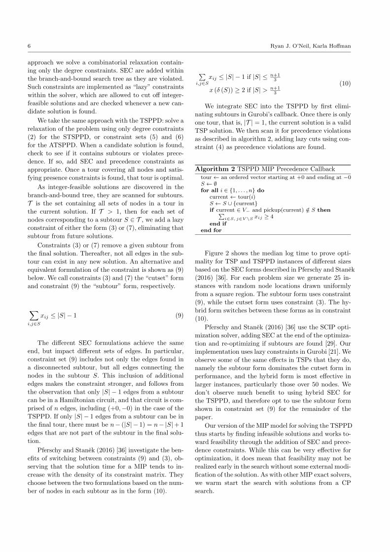
We integrate SEC into the TSPPD by first elimi-
nating subtours in Gurobi’s callback. Once there is only
one tour, that is, |T | = 1, the current solution is a valid
TSP solution. We then scan it for precedence violations
as described in algorithm 2, adding lazy cuts using con-
straint (4) as precedence violations are found.
Algorithm 2 TSPPD MIP Precedence Callbacktour ← an ordered vector starting at +0 and ending at −0S ← ∅for all i ∈ {1, . . . , n} do
current ← tour(i)S ← S ∪ {current}if current ∈ V− and pickup(current) /∈ S then∑
i∈S, j∈V \S xij ≥ 4
end ifend for
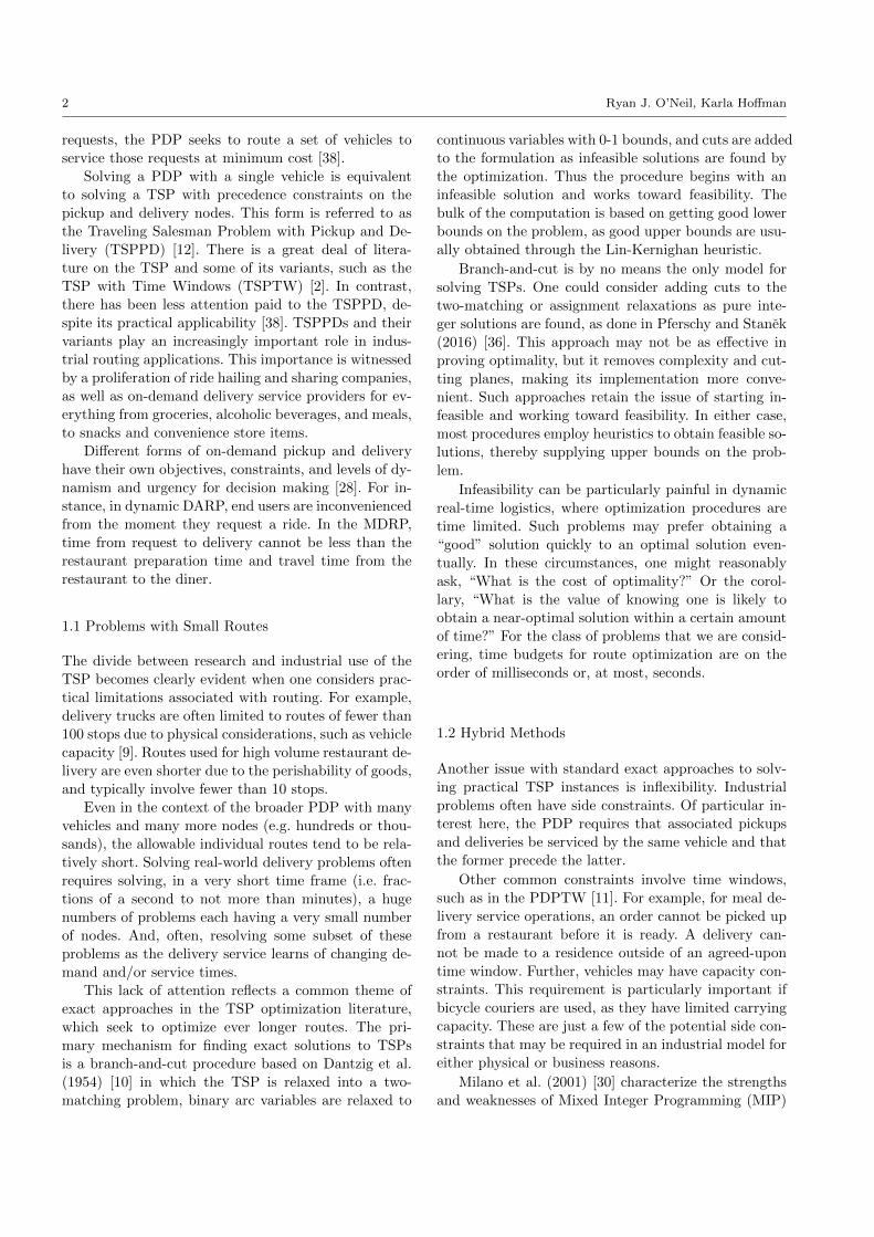
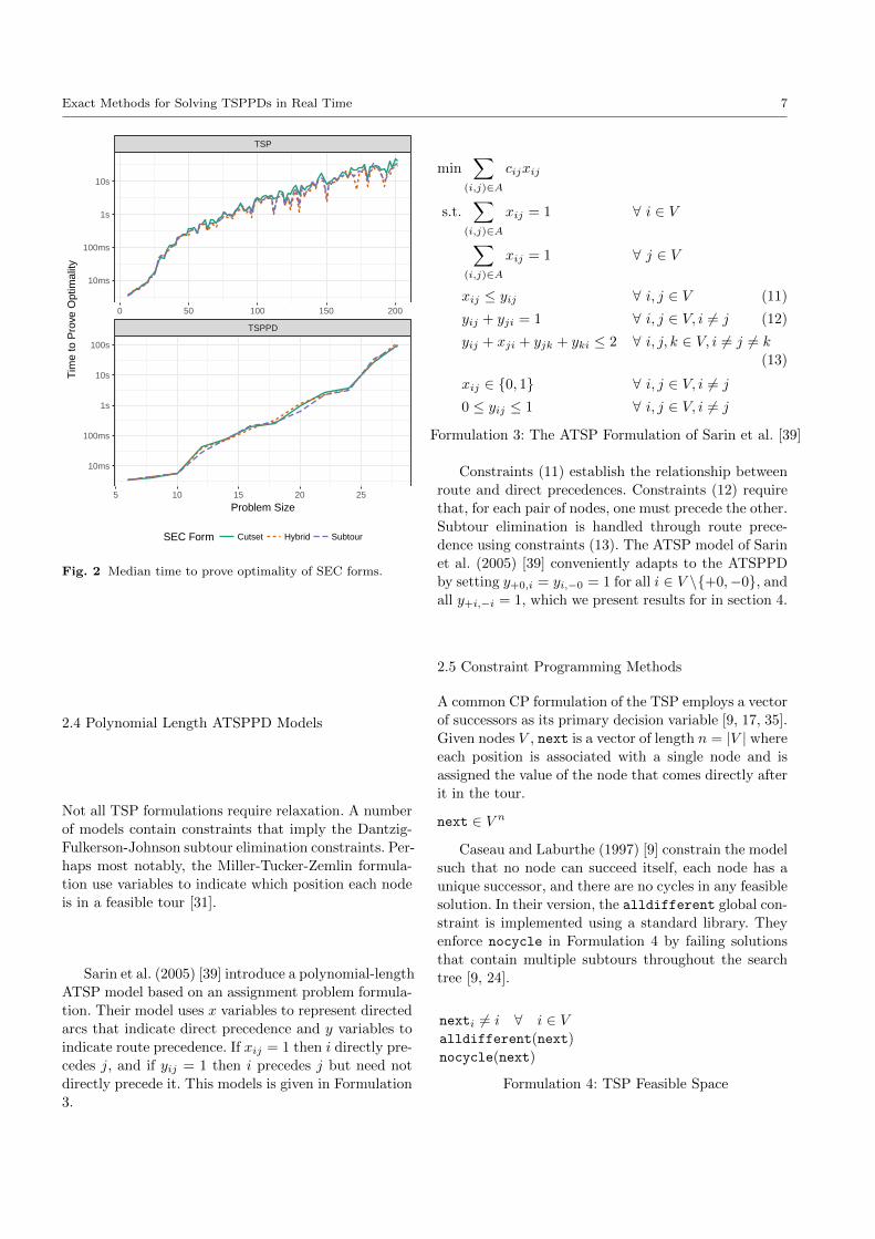
Figure 2 shows the median log time to prove opti-
mality for TSP and TSPPD instances of different sizes
based on the SEC forms described in Pferschy and Stanek
(2016) [36]. For each problem size we generate 25 in-
stances with random node locations drawn uniformly
from a square region. The subtour form uses constraint
(9), while the cutset form uses constraint (3). The hy-
brid form switches between these forms as in constraint
(10).
Pferschy and Stanek (2016) [36] use the SCIP opti-
mization solver, adding SEC at the end of the optimiza-
tion and re-optimizing if subtours are found [29]. Our
implementation uses lazy constraints in Gurobi [21]. We
observe some of the same effects in TSPs that they do,
namely the subtour form dominates the cutset form in
performance, and the hybrid form is most effective in
larger instances, particularly those over 50 nodes. We
don’t observe much benefit to using hybrid SEC for
the TSPPD, and therefore opt to use the subtour form
shown in constraint set (9) for the remainder of the
paper.
Our version of the MIP model for solving the TSPPD
thus starts by finding infeasible solutions and works to-
ward feasibility through the addition of SEC and prece-
dence constraints. While this can be very effective for
optimization, it does mean that feasibility may not be
realized early in the search without some external modi-
fication of the solution. As with other MIP exact solvers,
we warm start the search with solutions from a CP
search.
Exact Methods for Solving TSPPDs in Real Time 7
TSPPD
TSP
5 10 15 20 25
0 50 100 150 200
10ms
100ms
1s
10s
10ms
100ms
1s
10s
100s
Problem Size
Tim
e to
Pro
ve O
ptim
ality
SEC Form Cutset Hybrid Subtour
Fig. 2 Median time to prove optimality of SEC forms.
2.4 Polynomial Length ATSPPD Models
Not all TSP formulations require relaxation. A number
of models contain constraints that imply the Dantzig-
Fulkerson-Johnson subtour elimination constraints. Per-
haps most notably, the Miller-Tucker-Zemlin formula-
tion use variables to indicate which position each node
is in a feasible tour [31].
Sarin et al. (2005) [39] introduce a polynomial-length
ATSP model based on an assignment problem formula-
tion. Their model uses x variables to represent directed
arcs that indicate direct precedence and y variables to
indicate route precedence. If xij = 1 then i directly pre-
cedes j, and if yij = 1 then i precedes j but need not
directly precede it. This models is given in Formulation
3.
min∑
(i,j)∈A
cijxij
s.t.∑
(i,j)∈A
xij = 1 ∀ i ∈ V
∑(i,j)∈A
xij = 1 ∀ j ∈ V
xij ≤ yij ∀ i, j ∈ V (11)
yij + yji = 1 ∀ i, j ∈ V, i 6= j (12)
yij + xji + yjk + yki ≤ 2 ∀ i, j, k ∈ V, i 6= j 6= k
(13)
xij ∈ {0, 1} ∀ i, j ∈ V, i 6= j
0 ≤ yij ≤ 1 ∀ i, j ∈ V, i 6= j
Formulation 3: The ATSP Formulation of Sarin et al. [39]
Constraints (11) establish the relationship between
route and direct precedences. Constraints (12) require
that, for each pair of nodes, one must precede the other.
Subtour elimination is handled through route prece-
dence using constraints (13). The ATSP model of Sarin
et al. (2005) [39] conveniently adapts to the ATSPPD
by setting y+0,i = yi,−0 = 1 for all i ∈ V \{+0,−0}, and
all y+i,−i = 1, which we present results for in section 4.
2.5 Constraint Programming Methods
A common CP formulation of the TSP employs a vector
of successors as its primary decision variable [9, 17, 35].
Given nodes V , next is a vector of length n = |V | where
each position is associated with a single node and is
assigned the value of the node that comes directly after
it in the tour.
next ∈ V n
Caseau and Laburthe (1997) [9] constrain the model
such that no node can succeed itself, each node has a
unique successor, and there are no cycles in any feasible
solution. In their version, the alldifferent global con-
straint is implemented using a standard library. They
enforce nocycle in Formulation 4 by failing solutions
that contain multiple subtours throughout the search
tree [9, 24].
nexti 6= i ∀ i ∈ Valldifferent(next)
nocycle(next)
Formulation 4: TSP Feasible Space
8 Ryan J. O’Neil, Karla Hoffman
Some modern constraint solvers such as Gecode pro-
vide a circuit constraint, which efficiently handles prop-
agation for all of these and guarantees that a vector
forms a Hamiltonian circuit in any feasible solution
[19, 24]. Using this constraint simplifies the model.
circuit(c, next, z)
The circuit constraint accepts a variable into which
it propagates the total circuit length, along with a ma-
trix of arc costs [19]. Therefore the feasible set and ob-
jective function of the TSP can be fully represented
using the fairly simple CP Formulation 5.
min z
s.t. circuit(c, next, z)
next ∈ V n
Formulation 5: Circuit-Based TSP Formulation
Formulation 5 is advantageous in that it fully de-
scribes the TSP for n nodes. No additional constraints
related to subtour elimination need to be generated dur-
ing search. At each step in the search tree, constraint
propagation maintains a domain relaxation of the next
vector that has not been proven infeasible. If any ele-
ment of that vector is reduced to an empty domain, the
solver fails that section of the search tree and continues
its search elsewhere.
When it comes to the pickup and delivery portion
of the TSPPD, there is less clarity in the modeling ap-
proach. Well studied constraints exist in the CP litera-
ture for implementing value precedence on vectors [25].
However, these constraints do not operate on successorvectors such as next.
Implementations of precedence on circuits are de-
scribed in general terms in the CP literature in rela-
tion to the TSP with time windows (TSPTW), and
rely on the computation of times for node arrivals and
comparison of those arrival or execution times to feasi-
ble windows [5]. These formulations enforce precedence
among pickup and delivery pairs using the cost of the
tour upon visiting each node. A delivery’s cost must be
at least that of its associated pickup plus the cost of
traveling along their connecting arc. We refer to this as
“cost-based precedence”.
Such a formulation is intended to operate on TSPs
where there are time windows during which events must
occur. This concept is not found in the pure TSPPD,
in which precedence may be more directly modeled on
circuits using set-based variables and constraints.
The most complete description we have found of a
precedence constraint which solely encodes the prece-
dence relations in a circuit is described in Focacci et
al. (2002) [16]. Their formulation maintains predecessor
and successor sets for each node. They use this mecha-
nism to detect when additional nodes must be inserted
between node pairs, and to assist in domain reduction
on the next vector. We adapt and formalize this repre-
sentation for the TSPPD in section 3.2 and compare it
to the cost-based precedence used for the TSPTW.
2.5.1 Branching and Propagation
A CP solver’s search over a model’s feasible space is
guided by branching on variable domains. At each branch
point, the domains of a variable or set of variables
are reduced. The constraints of the model propagate
these changes into the domains of other variables in
the model that are either directly or indirectly related
to the branching variables. When a variable’s domain
is reduced to a single value, it is assigned that value
for any nodes further down the search tree. If propaga-
tion reduces a variable’s domain to the empty set, that
segment of the search tree fails and is removed from
consideration.
Unlike MIP solvers that obtain lower bounds from
the LP relaxation, CP solvers traditionally do not natu-
rally include a mechanism for obtaining relaxation bounds
for the problem. Instead, VP uses propositional logic
and clever search techniques to fathom major parts of
the tree and is often stopped as soon as a feasible so-
lution is found. Thus, it is more often used as a satis-
fiability algorithm than as an optimization procedure.
There are some papers that explore the integration of
reduced cost and dual bound computations into CP
search [16, 17, 30]. We present test results for such for-
mulations in section 4.
It is well established that the path or circuit con-
straints of CP solvers are not effective at finding opti-
mal TSP solutions on their own [17]. In order to aid
the optimization process, we direct the search through
branching rules and additional propagation based on
objective value bounds. As has long been understood
with MIP, dynamic variable selection is fundamental
to fast solution of problems in CP, particularly when
such problems require optimization of some objective
function [35].
Often, CP modelers adopt heuristic techniques to
determine variable branching order and choose the most
profitable assignments. One such variable selection tech-
nique is the first-fail heuristic, in which the variable
with the smallest domain at the current point in the
search tree is branched on, generating early failures in
an attempt to fathom sections of the search tree quickly.
Both Caseau and Laburthe (1997) [9] and Pesant et
al. (1998) [35] use first-fail as a component in their
Exact Methods for Solving TSPPDs in Real Time 9
branching schemes to select among the unassigned next
variables.
Pesant et al. (1998) [35] use a branching strategy
that adds a tie-breaking rule to first-fail. If two
variables have the same, minimal, domain cardinality,
they select the one that appears in more domains of
other unassigned variables. They then assign successor
nodes to the branching variable in increasing order of
their cost, measured by the arc cost incurred by fixing
the connection between the branching variable and its
assigned successor.
Caseau and Laburthe (1997) [9] offer a more sophis-
ticated branching scheme, which incorporates a regret
heuristic. At each node in the search tree, the regret
for any unassigned node i in the next vector is the dif-
ference between its two closest, or lowest cost, feasible
assignments, j1 and j2, as shown in equation (14).
regret(i) = |cij1 − cij2 | (14)
Branching on variable regret can help a CP solver
make good choices early in the search. Consistent with
this idea is the view of regret as an approximation of re-
duced costs of an assignment problem (AP) relaxation
of the TSP [17]. A weakness of the regret heuristic is
that it is not as straightforward in adapting to side con-
straints as some others, such as closest neighbor (CN),
which implements a pure greedy strategy. CN branch-
ing is easily modified to respect innately precedence
rules by starting at +0 and always branching on the
least cost feasible arc at the end of the current partial
route. We call this branching scheme Sequential Clos-
est Neighbor (SCN). Regret branching is not so easily
adapted, in our experience, and requires effective prop-
agation using decisions made about partial routes.
2.5.2 Bounding Techniques
A particular difficulty in using CP techniques for opti-
mization is the handling of objective functions. A stan-
dard approach is to assign a variable to the objective
value. When a new incumbent solution is found, we re-
quire that all subsequent solutions be better than our
best known solution. Meanwhile, as other variable do-
mains are restricted as a result of choices in the search
tree, lower bounds are set on the objective variable.
This allows the solver to fathom sections of the search
tree that cannot perform as well as the current incum-
bent solution [17]. In a CP system such as Gecode, this
requires adding a constraint on the cost z < z∗ when
a new incumbent solution with cost z∗ is discovered in
the search tree.
Caseau and Laburthe (1997) [9] and Pesant et al.
(1998) [35] explore three different mechanisms for es-
tablishing lower bounds on TSP cost at each branch in
the search tree. CN bounds are computed by summing
the cost of assigning each node to the closest node in
its domain. These bounds are easy to compute, but my-
opic and tend not to be tight. Such bounds are easily
computed as part of variable domain propagation in the
circuit constraint, and thus do not require an explicit
representation.
More sophisticated bounds involve computing a Min-
imum Spanning Tree (MST) over the domain of the
next vector. A MST does not require that its solu-
tion form a tour and thus underestimates the cost of
the TSP. Computing MSTs is fast and it is possible to
quickly update the solutions within the search tree us-
ing an incremental form of Kruskal’s algorithm [9, 35].
Alternatively, one can derive bounds from a Mini-
mum Spanning Arborescence (MSA) over the domain
of the next vector. A MSA forms a directed spanning
tree from the root towards its leaves. MSAs can be com-
puted in O(EV ) time using Edmonds’ algorithm [13].
More recent refinements of the algorithm can also be
deployed that find an MSA in O(E + V log V ) time
[18].
Focacci et al. (1999) [17] and Focacci et al. (2002)
[16] explore the idea of using relaxations during the
search that provide both dual bounds and reduced cost
information for variable fixing and triggering further
propagation. They implement an Assignment Problem
(AP) relaxation of the TSP using the feasible domain
of next in the search tree, and another vector prev,
which is the inverse of next. Only feasible arcs at the
current location in the search tree are included in the
AP relaxation.
The AP relaxation can be solved in O(n3) time at
the root node in the search tree, and in O(n2) time upon
domain changes throughout the tree using augmenting
path steps [8]. A reduced cost matrix is computed as
part of these updates, and can be then used to prune
variable domains from next. Empirical results show this
technique is more efficient with respect to solution time
than MST-based dual bounds due to its relatively low
computational complexity [16, 17].
2.5.3 Additive Bounding & 1-Tree Relaxations
Benchimol et al. (2012) [4] explore techniques to in-
crease filtering of weighted circuit constraints by com-
bining AP relaxations with 1-tree relaxations obtained
from Held-Karp bounds [22, 23]. They combine these
two relaxations within the additive bounding frame-
work of Fischetti and Toth (1992) [14]. This procedure
10 Ryan J. O’Neil, Karla Hoffman
uses one relaxation to compute an initial dual bound
and set of reduced costs, then applies subsequent re-
laxations of different forms directly to the reduced cost
matrix resulting from the initial relaxation. The final
dual bound is the sum of the objective values of the var-
ious relaxations. The reduced cost matrix is provided
by the final relaxation applied [14].
Additive bounding can provide tighter dual bounds
than individual relaxations because each relaxation in-
corporates different constraints from the original model.
For instance, an AP relaxation has degree constraints
but will allow subtours, while a 1-tree relaxation dis-
allows subtours while not enforcing degree constraints.
Combining the relaxations can enhance filtering inside
a CP search and may result in dramatically smaller
search trees, as shown in Benchimol et al. (2012) [4].
We attempt to improve the runtime of our CP mod-
els against TSPPD instances using a similar technique.
However, while incremental AP relaxations fit easily
into real-time optimization since AP updates require
a single execution of an O(n2) algorithm with each
relevant variable domain change, adapting 1-tree re-
laxations to the demands of real-time systems is not
so straightforward. Computing an optimal 1-tree re-
laxation requires repeated applications of an algorithm
such as Kruskal’s, each of which runs in O(m log n) time
[4, 40].
Detecting convergence of the 1-tree bound is non-
trivial and based on subgradient techniques [15]. Each
iteration involves calculating node potentials which pe-
nalize nodes that do not have a degree of two, as in
(15). tm is the current step size, while dmi is the de-
gree of node i in iteration m. The node potentials π
are added into the edge costs for the next 1-tree as
cij + πi + πj , where cij is the original edge cost. Since
a TSP tour incurs each node potential cost twice, the
TSP is invariant to these node potentials, while the 1-
tree is not [23]. Converting a 1-tree bound into a TSP
bound simply involves subtracting each node potential
twice from the 1-tree cost.
π1i = 0 ∀ 1 ≤ i ≤ nπm+1i = πm
i + tm(dmi − 2) ∀ 1 ≤ i ≤ n (15)
A number of mechanisms exist for updating the step
size tm. We compute 1-trees using a fixed number of
iterations, as outlined in Valenzuela and Jones (1997)
[40]. The formula (16) gives a step size update that
works on a fixed number of iterations, where L1 is the
first 1-tree objective value, m is the current iteration,
M is the total number of iterations, and n is the number
of nodes in the graph.
●●●
●
●●
●
●●
●
●●
●
●●
●
●
●
●
●
●
●
●●
●
●●
●
●●
●
●●
●
●●
●
●
●
●
●
●
●
●●
●●●
●
●●
●
●●
●
●●
●
●
●
●
●●
●
●●
●
●
●
●
●
●
●
●
●
●
●●
●
●
●
●
●●
Maximum
Median
10 20 30
10 20 30
0
5
10
15
0
10
20
Problem Size
Opt
imal
ity G
ap o
f Hel
d−K
arp
Bou
nd (
%)
Iterations 5 10 25 Type ● TSP TSPPD
Fig. 3 Optimality gap of Held-Karp bounds.
t1 = 12nL
1
tm = t1(
(m− 1) 2M−52(M−1) − (m− 2) + (m−1)(m−2)
2(M−1)(M−2)
)(16)
The Held-Karp bound at a node in the CP search
is thus the maximum objective in terms of the origi-
nal edge costs from a series of M 1-tree computations.
Variable domain filtering can be accomplished using
either marginal costs per Benchimol et al. (2010) [3]
or by computing reduced costs directly. While we ob-
serve both improvements in runtime and search tree size
for TSP instances using the 1-tree relaxation and addi-
tive bounding, those benefits do not translate readily to
TSPPD instances in our implementation. This appears
to be because the 1-tree bounds degrade significantly
in the presence of precedence constraints.
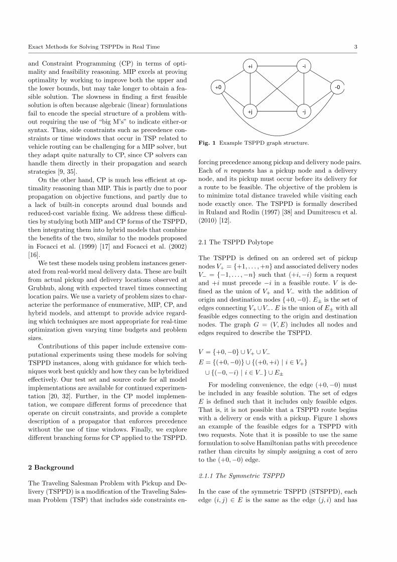
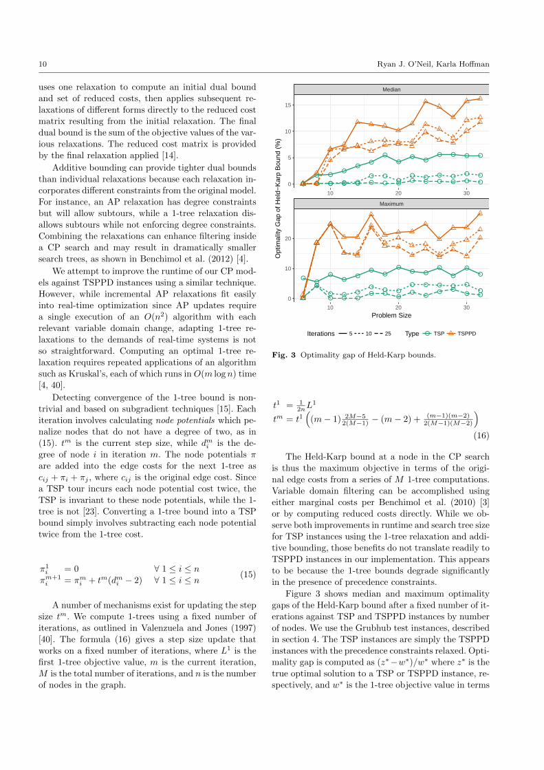
Figure 3 shows median and maximum optimality
gaps of the Held-Karp bound after a fixed number of it-
erations against TSP and TSPPD instances by number
of nodes. We use the Grubhub test instances, described
in section 4. The TSP instances are simply the TSPPD
instances with the precedence constraints relaxed. Opti-
mality gap is computed as (z∗−w∗)/w∗ where z∗ is the
true optimal solution to a TSP or TSPPD instance, re-
spectively, and w∗ is the 1-tree objective value in terms
Exact Methods for Solving TSPPDs in Real Time 11
of the original edge costs at the root node of the search
tree after a fixed number of iterations.
We observe that, as problem size grows, the Held-
Karp bound remains quite good for TSP instances, while
degrading quickly for TSPPD instances. In the update
mechanism we use, the benefit of increasing the number
of iterations drops sharply from 25 to 100. Further, the
spread of the optimality gap appears to decrease for the
TSP with increased iterations, but not for the TSPPD.
We believe that this challenge is due to the structure
of the Held-Karp bound when applied to TSPPD in-
stances. The bound itself is based on undirected graphs,
while the TSPPD is fundamentally a directed problem
(pickups must precede deliveries). Results against TSP
instances indicate that adapting the Held-Karp bound
to the TSPPD may be a worthy endeavor, but we do
not consider it further in this paper.
3 Approach
Our goal in this study is not to directly compare MIP
and CP methods. While the latter can outperform MIP
for certain problem classes, MIP solvers have been tra-
ditionally designed and built expressly for optimization.
Rather, we hope to observe the impact of pickup and
delivery structure applied to small TSPPD instances
which must be solved in “real time”, when high quality
routes must be constructed within seconds or millisec-
onds in response to events during an operational period.
Intuitively, we understand that additional constraints
complicate the search for MIP solvers, while support-
ing it for CP. It is less clear how precedence impacts
solution time, and whether those solution times can be
improved through hybridization, i.e. using components
of more than one standard algorithm.
3.1 Mixed Integer Programming TSPPD Models
We base our MIP implementation of the TSPPD solver
on that of Pferschy and Stanek (2016). There are a few
points where our underlying TSP implementation di-
verges from theirs. First, they use the SCIP solver as
their optimization engine, while we use Gurobi [21, 29].
They mention the possibility of using lazy constraints
for SEC but do not actually implement and test this ap-
proach. We implement subtour elimination inside lazy
constraints using inequality (9) in our implementation
and precedence constraints using inequality (4).
Once a single tour is found in the search tree, we
scan it for precedence constraint violations. If a partial
route S exists such that +0,−i ∈ S and −0,+i /∈ S, we
add a lazy constraint using inequality (4). This results
in model (1).
Algorithm 2 detects precedence violations given fea-
sible tours by starting at +0 and following the directed
tour from that node. If it finds a delivery that oc-
curs before its associated pickup, it adds a lazy con-
straint. For comparison, we also test the asymmetric
polynomial-length model in Formulation 3 with prece-
dence of pickup and delivery pairs enforced by setting
y+i,−i = 1 for each pair (+i,−i).
3.2 Constraint Programming TSPPD Model
3.2.1 Cost-Based Circuit Precedence
The addition of pickup and delivery precedence rela-
tions to the CP TSP model requires a constraint that
fails the search tree when they are violated and removes
infeasible values from variable domains in response to
branching decisions. Berbeglia et al. (2012) [5] give a
formulation that enforces precedence using the times
that events occur, a common structure in TSPTW mod-
els.
Since the pure form of the TSPPD does not include
time windows, we think of this as cost-based prece-
dence, as formulated in (17). A cost vector encodes
the cumulative route cost at every node. Each delivery
−i ∈ V− must have a cost greater than or equal to its
associated pickup +i.
min z
s.t. circuit(c, next, z)
circuit-precede-cost(next, cost)
next−0 = +0
cost+0 = 0
cost−i ≥ cost+i ∀ +i ∈ V+next ∈ V n
cost ∈ Nn
z ≥ max cost
(17)
A custom propagator circuit-precede-cost de-
tects when a branching decision is made such that nexti =
j in the search tree, either directly through branching
or as a result of propagation. The assignment of next−0is required by the model and ignored during propaga-
tion. When any other variable nexti is assigned a value
j in the search tree, the cost i must now be equal to
the cost of j plus the cost of their connecting arc. This
is achieved through a local constraint of the form (18).
nexti = j =⇒ costj = costi + cij (18)
12 Ryan J. O’Neil, Karla Hoffman
3.2.2 Set-Based Circuit Precedence
It is also possible to enforce precedence more directly
using set variables, as Focacci et al. (2002) [16] out-
line. Our implementation uses vectors of predecessor
and successor nodes called pred and succ, respectively,
that track which nodes must and must not precede and
succeed each node based on the current structure of par-
tial routes in the solution. The TSPPD CP formulation
using set precedence is shown in Formulation 19.
A custom propagator circuit-precede-set is trig-
gered whenever an assignment to next is made. The ori-
gin node, +0, must have an empty set of predecessors,
while the destination node, −0, must have an empty set
of successors. No node’s predecessor and successor sets
are allowed to intersect. A pickup’s successor set must
be a superset of its associated delivery’s successor set,
and the delivery’s predecessor set must be a superset of
the pickup’s predecessor set.
min z
s.t. circuit(next, z)
circuit-precede-set(next, pred, succ)
next−0 = +0
+i ∈ pred−i ∀ −i ∈ VD−i ∈ succ+i ∀ +i ∈ VPpredi ∩ succi = ∅ ∀ i ∈ Vpred−i ⊂ pred+i ∀ +i ∈ V+succ+i ⊂ succ−i ∀ +i ∈ V+pred+0 = ∅succ−0 = ∅next ∈ V n
pred ∈ {V n}nsucc ∈ {V n}nz ≥ 0
(19)
The assignment of next−0 is required by the model
and ignored during propagation. When any other vari-
able nexti is assigned a value j in the search tree, the
successor set for i must now be equal to the successor
set of j with the addition of j itself. Similarly, the prede-
cessor set of j must now be equal to the predecessor set
of i with the addition of i. Our circuit-precede-set
constraint shown in (20) accomplishes this by adding
local constraints to the current branch of the search
tree upon assignment of any nexti.
nexti = j =⇒ predj = predi ∪ {i}succi = succj ∪ {j}
(20)
next+i = +j =⇒ −i ∈ succ+j
−j ∈ succ+i
next+i = −j =⇒ −i ∈ succ+j
−i ∈ succ−j+j ∈ pred+i
+j ∈ pred−i
next−i = +j =⇒ +i ∈ pred+j
+i ∈ pred−j−j ∈ succ+i
−j ∈ succ−i
next−i = −j =⇒ +i ∈ pred−j+j ∈ pred−i
(21)
Further propagation is accomplished by explicitly
adding to and removing values from the predecessor
and successor sets upon propagation of nexti = j, de-
pending on the values of i and j and what is known
about their precedence relations, as shown in (21). This
allows failures to be detected early in the search tree.
Set-based precedence operates directly on precedence
structure and does not require time windows. However,
it may be beneficial to combine both forms in cases
where there is precedence structure and time windows
on event times. We study a final form of precedence
constraint that combines the cost and set-based form
by simply applying both of them.
3.3 Hybrid TSPPD Models
Milano et al. (2001) [30] characterize the benefits of
incorporating optimization procedures and CP into the
same framework. We attempt two hybrid methods for
tackling the TSPPD. In the first, we incorporate AP
relaxations for reduced cost variable fixing into our CP
TSPPD model, similar to its application to the TSPTW
by Focacci et al. (2002) [16]. In the second, we attempt
to combat the issue of MIP starting its search far from
feasibility by using a CP model to find solutions quickly,
and warm-starting the MIP solver with the best known
solution after a given time limit.
3.3.1 Reduced Cost-Based Domain Filtering
We implement reduced cost-based variable fixing as a
custom propagator inside of Gecode CP framework.
The propagator subscribes to value assignments on each
index of the next vector. When first triggered, the prop-
agator initializes and solves the primal-dual AP solving
Exact Methods for Solving TSPPDs in Real Time 13
algorithm of Carpaneto et al. (1988) [8], an operation
that takes O(n3) time. When subsequent assignments
to next occur in the search tree, the propagator per-
forms an augmenting path update in O(n2) time.
The custom propagator tracks which variables are
currently unassigned. When a branching decision is made
such that nexti = j, the propagator forces the primal-
dual algorithm to set row i to column j in its internal
matrix, and removes any conflicting assignments from
consideration. For each unassigned variable nexti and
each j in the domain of nexti, the AP relaxation pro-
vides a reduced cost rcij . It also provides a dual bound
w∗ for the objective function of the TSPPD at that lo-
cation in the search tree. If, for any feasible arc (i, j),
w∗ + rcij ≥ z, where z is the upper bound on the ob-
jective function, we infer that nexti 6= j.
3.3.2 MIP Warm Starting
We study a second form of integration by using CP to
warm start MIP. As previously discussed in section 1.2,
side constraints can make MIP implementations take
longer to find feasible solutions. We address this behav-
ior by using our CP implementation to find good solu-
tions quickly, and then warm starting the MIP solver
with them. This not only provides primal bounds to the
MIP solver, but also gives it a neighborhood in which
to search. We test the warm starting technique using
different time budgets on the CP solver.
4 Results
We test enumerative, MIP, CP, and hybrid forms of
the TSPPD models using instances constructed from
pickup and delivery locations observed at Grubhub,
along with expected travel times connecting location
pairs. The test set has 10 instances per problem size.
This allows us to gauge the performance of the mod-
els on realistic problems from meal delivery, in which
pickup locations are likely to be clustered close together,
and there may be many near optimal solutions that
would have to be considered to prove optimality.
We evaluate the models according to multiple crite-
ria: the time taken to find a first feasible TSPPD route,
the time to find a route within 10% of the true opti-
mum, the time to find an optimal route, and the time
to prove optimality. The first three measures are im-
portant to real-time logistics, where high quality routes
must be found quickly and there may not be enough
time to optimize fully. The final measure quantifies the
capacity of model formulations and algorithms to opti-
mize. We use time to prove optimality as a proxy for
general algorithmic performance while selecting config-
urations. Not all modeling techniques surveyed have ac-
cess to global dual bounds, so we measure optimality
gap of primal solutions from the true optimum.
Charts report the median and maximum of execu-
tion times for each problem size and model configura-
tion with the vertical axis scaled to log time. These
measures are useful in choosing models for production
systems because they give us a sense of typical per-
formance and poor performance in terms of execution
time. Given a target problem size and time budget, we
can use the results of these test to determine the best
approach for a given TSPPD problem size. Execution
times are limited to 1000 seconds. Any model configu-
ration that is not able to achieve a particular goal (e.g.
finding a feasible solution, or finding a solution with
10% of optimal) for all instances of a given size is re-
moved from consideration for that problem size, causing
its line to end on the graph.
We generate results using Gurobi 8.0.0 as the MIP
solver and Gecode 6.0.1 for the CP models. Model code
is written using C++14. The test machine is a Lenovo
X1 Carbon with a 4-core Intel Core i5 CPU and 16
GB of RAM. We test using 1 thread and 4 threads, but
concurrency does not appear to change our conclusions,
so we report results for a single thread. Single-threaded
executions of these models are deterministic and thus
easier to interpret and compare.
Sections 4.1 and 4.2 discuss the testing of the CP al-
ternatives. Section 4.3 then similarly discusses our test-
ing of MIP models. Finally, section 4.4 provides results
that compare enumeration to the best CP and best MIP
models.
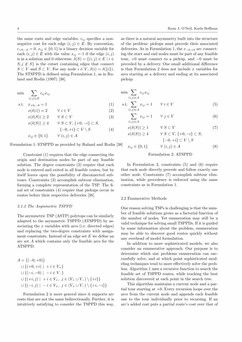
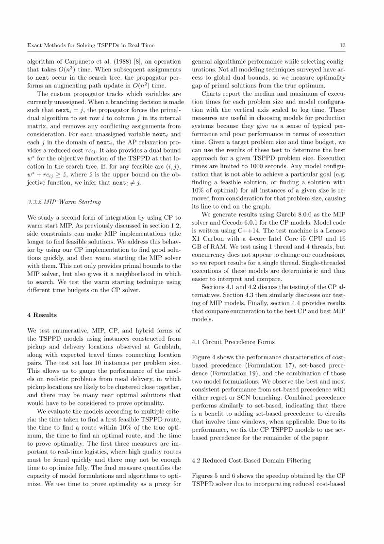
4.1 Circuit Precedence Forms
Figure 4 shows the performance characteristics of cost-
based precedence (Formulation 17), set-based prece-
dence (Formulation 19), and the combination of those
two model formulations. We observe the best and most
consistent performance from set-based precedence with
either regret or SCN branching. Combined precedence
performs similarly to set-based, indicating that there
is a benefit to adding set-based precedence to circuits
that involve time windows, when applicable. Due to its
performance, we fix the CP TSPPD models to use set-
based precedence for the remainder of the paper.
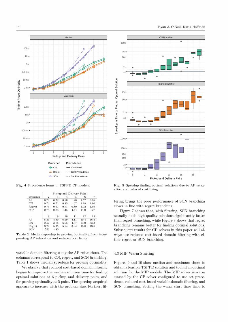
4.2 Reduced Cost-Based Domain Filtering
Figures 5 and 6 shows the speedup obtained by the CP
TSPPD solver due to incorporating reduced cost-based
14 Ryan J. O’Neil, Karla Hoffman
●
●●
●
●
●
●
●
●●
●
●
●
●
●●
●
●
●
●
●
●
●
●
●
●●
●
●
●
●
●
●
●●
●
● ●
●
●●
●
●
●
Maximum
Median
2 3 4 5 6 7 8 9
1ms
10ms
100ms
1s
10s
100s
1ms
10ms
100ms
1s
10s
100s
Pickup and Delivery Pairs
Tim
e to
Pro
ve O
ptim
ality
Brancher● CN
Regret
SCN
Precedence
Combined
Cost Precedence
Set Precedence
Fig. 4 Precedence forms in TSPPD CP models.
Pickup and Delivery PairsBrancher 2 3 4 5 6 7All 0.74 0.72 0.90 1.20 1.57 3.98CN 0.74 0.71 0.85 1.07 1.18 1.80Regret 0.75 0.67 0.71 0.80 1.02 1.59SCN 0.74 0.83 1.45 4.44 14.0 127
8 9 10 11 12 13All 8.35 4.89 6.69 4.11 19.4 16.2CN 2.52 3.76 6.95 4.37 23.0 53.3Regret 3.24 5.35 5.94 3.84 16.8 13.6SCN 520 480
Table 1 Median speedup to proving optimality from incor-porating AP relaxation and reduced cost fixing.
variable domain filtering using the AP relaxations. The
columns correspond to CN, regret, and SCN branching.
Table 1 shows median speedups for proving optimality.
We observe that reduced cost-based domain filtering
begins to improve the median solution time for finding
optimal solutions at 6 pickup and delivery pairs, and
for proving optimality at 5 pairs. The speedup acquired
appears to increase with the problem size. Further, fil-
SCN Brancher
Regret Brancher
CN Brancher
2 4 6 8 10 12
1x
2x
10x
25x
100x
1x
2x
10x
25x
1x2x
10x
25x
100x
1000x
Pickup and Delivery Pairs
Spe
edup
in T
ime
to F
ind
an O
ptim
al S
olut
ion
Fig. 5 Speedup finding optimal solutions due to AP relax-ation and reduced cost fixing.
tering brings the poor performance of SCN branching
closer in line with regret branching.
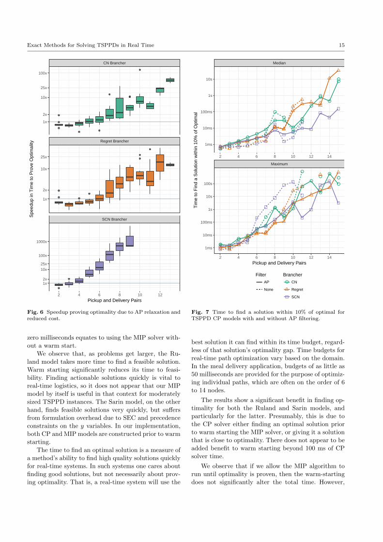
Figure 7 shows that, with filtering, SCN branching
actually finds high quality solutions significantly faster
than regret branching, while Figure 8 shows that regret
branching remains better for finding optimal solutions.
Subsequent results for CP solvers in this paper will al-
ways use reduced cost-based domain filtering with ei-
ther regret or SCN branching.
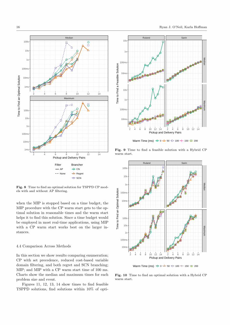
4.3 MIP Warm Starting
Figures 9 and 10 show median and maximum times to
obtain a feasible TSPPD solution and to find an optimal
solution for the MIP models. The MIP solver is warm
started by the CP solver configured to use set prece-
dence, reduced cost-based variable domain filtering, and
SCN branching. Setting the warm start time time to
Exact Methods for Solving TSPPDs in Real Time 15
SCN Brancher
Regret Brancher
CN Brancher
2 4 6 8 10 12
1x
2x
10x
25x
100x
1x
2x
10x
25x
1x2x
10x25x
100x
1000x
Pickup and Delivery Pairs
Spe
edup
in T
ime
to P
rove
Opt
imal
ity
Fig. 6 Speedup proving optimality due to AP relaxation andreduced cost.
zero milliseconds equates to using the MIP solver with-
out a warm start.
We observe that, as problems get larger, the Ru-
land model takes more time to find a feasible solution.
Warm starting significantly reduces its time to feasi-
bility. Finding actionable solutions quickly is vital to
real-time logistics, so it does not appear that our MIP
model by itself is useful in that context for moderately
sized TSPPD instances. The Sarin model, on the other
hand, finds feasible solutions very quickly, but suffers
from formulation overhead due to SEC and precedence
constraints on the y variables. In our implementation,
both CP and MIP models are constructed prior to warm
starting.
The time to find an optimal solution is a measure of
a method’s ability to find high quality solutions quickly
for real-time systems. In such systems one cares about
finding good solutions, but not necessarily about prov-
ing optimality. That is, a real-time system will use the
●●
●●
●●
● ●
●
●
●
●●
●
●●
●●
●
●
●
●
●
●
●
●
● ●
● ●
●●
●
●
●
●
●
●
●
●
●●
●
●
●
●
●
●
●
●
● ●
Maximum
Median
2 4 6 8 10 12 14
2 4 6 8 10 12 14
1ms
10ms
100ms
1s
10s
1ms
10ms
100ms
1s
10s
100s
Pickup and Delivery Pairs
Tim
e to
Fin
d a
Sol
utio
n w
ithin
10%
of O
ptim
al
Filter
AP
None
Brancher● CN
Regret
SCN
Fig. 7 Time to find a solution within 10% of optimal forTSPPD CP models with and without AP filtering.
best solution it can find within its time budget, regard-
less of that solution’s optimality gap. Time budgets for
real-time path optimization vary based on the domain.
In the meal delivery application, budgets of as little as
50 milliseconds are provided for the purpose of optimiz-
ing individual paths, which are often on the order of 6
to 14 nodes.
The results show a significant benefit in finding op-
timality for both the Ruland and Sarin models, and
particularly for the latter. Presumably, this is due to
the CP solver either finding an optimal solution prior
to warm starting the MIP solver, or giving it a solution
that is close to optimality. There does not appear to be
added benefit to warm starting beyond 100 ms of CP
solver time.
We observe that if we allow the MIP algorithm to
run until optimality is proven, then the warm-starting
does not significantly alter the total time. However,
16 Ryan J. O’Neil, Karla Hoffman
●
●●
●
●
●
● ●
●
●
●●
●
●
●
●
●●
●
● ●
●
● ●
●
●
●●
●
● ●
●
● ●
●
●
●
●
Maximum
Median
2 4 6 8 10 12 14
2 4 6 8 10 12 14
1ms
10ms
100ms
1s
10s
100s
1ms
10ms
100ms
1s
10s
100s
Pickup and Delivery Pairs
Tim
e to
Fin
d an
Opt
imal
Sol
utio
n
Filter
AP
None
Brancher● CN
Regret
SCN
Fig. 8 Time to find an optimal solution for TSPPD CP mod-els with and without AP filtering.
when the MIP is stopped based on a time budget, the
MIP procedure with the CP warm start gets to the op-
timal solution in reasonable times and the warm start
helps it to find this solution. Since a time budget would
be employed in most real-time applications, using MIP
with a CP warm start works best on the larger in-
stances.
4.4 Comparison Across Methods
In this section we show results comparing enumeration;
CP with set precedence, reduced cost-based variable
domain filtering, and both regret and SCN branching;
MIP; and MIP with a CP warm start time of 100 ms.
Charts show the median and maximum times for each
problem size and event.
Figures 11, 12, 13, 14 show times to find feasible
TSPPD solutions, find solutions within 10% of opti-
●
●● ●
●●
● ●
●
●●
●
●
●
●●
●●
●
●
●●
●
●
●
●
●●
●●
●●
●● ●
●●
●●
●● ●
●●
●● ●
● ●●
● ●●
●
● ●
Ruland Sarin
Median
Maxim
um
2 4 6 8 10 12 14 2 4 6 8 10 12 14
10ms
100ms
1s
10s
10ms
100ms
1s
10s
Pickup and Delivery Pairs
Tim
e to
Fin
d a
Fea
sibl
e S
olut
ion
Warm Time (ms) ● 0 50 100 150 200
Fig. 9 Time to find a feasible solution with a Hybrid CPwarm start.
●●
● ●
●●
● ●●
●
●
●●
●● ●
●
● ●
●
●
●
●
●
●
●
●
●
●
●●
●
● ●
●
●●
●
●
●●
● ●
●
●
●
●
●● ●
Ruland Sarin
Median
Maxim
um
2 4 6 8 10 12 14 2 4 6 8 10 12 14
10ms
100ms
1s
10s
100s
10ms
100ms
1s
10s
100s
Pickup and Delivery Pairs
Tim
e to
Fin
d an
Opt
imal
Sol
utio
n
Warm Time (ms) ● 0 50 100 150 200
Fig. 10 Time to find an optimal solution with a Hybrid CPwarm start.
Exact Methods for Solving TSPPDs in Real Time 17
● ● ●● ● ● ● ●
● ● ● ● ● ●
●● ●
●● ●
●●
● ● ● ●●
●
Maximum
Median
2 4 6 8 10 12 14
2 4 6 8 10 12 14
1ms
10ms
100ms
1s
10s
1ms
10ms
100ms
1s
10s
Pickup and Delivery Pairs
Tim
e to
Fin
d a
Fea
sibl
e S
olut
ion
Solver● CP+AP (Regret)
CP+AP (SCN)
Enumeration
Ruland
Ruland+CP+AP (SCN)
Sarin
Sarin+CP+AP (SCN)
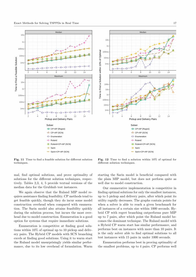
Fig. 11 Time to find a feasible solution for different solutiontechniques.
mal, find optimal solutions, and prove optimality of
solutions for the different solution techniques, respec-
tively. Tables 2,3, 4, 5 provide textual versions of the
median data for the Grubhub test instances.
We again observe that the Ruland MIP model re-
quires assistance finding feasibility. CP methods tend to
get feasible quickly, though they do incur some model
construction overhead when compared with enumera-
tion. The Sarin model also attains feasibility quickly
during the solution process, but incurs the most over-
head due to model construction. Enumeration is a good
option for systems that require immediate solutions.
Enumeration is competitive at finding good solu-
tions within 10% of optimal up to 10 pickup and deliv-
ery pairs. The Hybrid CP models with SCN branching
excels at finding good solutions. Using it to warm start
the Ruland model unsurprisingly yields similar perfor-
mance, due to its low overhead of formulation. Warm
● ●● ●
● ●
● ●
●
● ●●
●
●
● ● ●
●● ●
● ●
●●
●●
●
●
Maximum
Median
2 4 6 8 10 12 14
2 4 6 8 10 12 14
1ms
10ms
100ms
1s
10s
1ms
10ms
100ms
1s
10s
100s
Pickup and Delivery Pairs
Tim
e to
Fin
d a
Sol
utio
n w
ithin
10%
of O
ptim
al
Solver● CP+AP (Regret)
CP+AP (SCN)
Enumeration
Ruland
Ruland+CP+AP (SCN)
Sarin
Sarin+CP+AP (SCN)
Fig. 12 Time to find a solution within 10% of optimal fordifferent solution techniques.
starting the Sarin model is beneficial compared with
the plain MIP model, but does not perform quite as
well due to model construction.
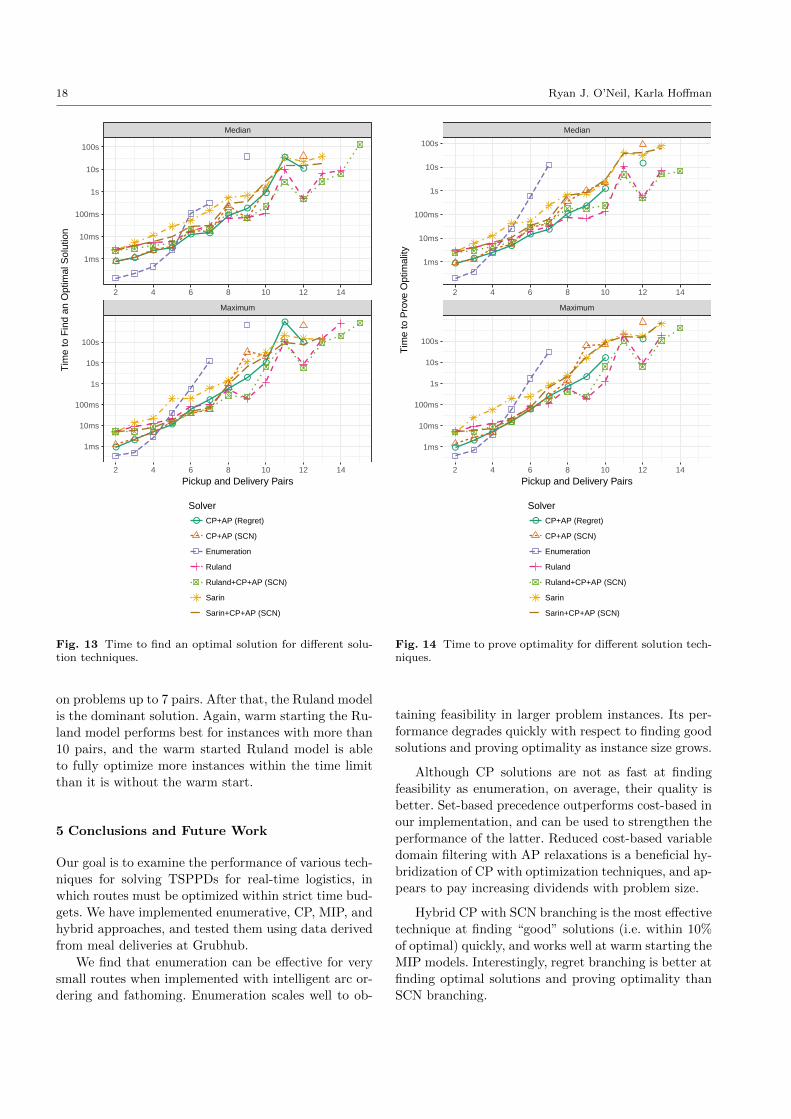
Our enumerative implementation is competitive in
finding optimal solutions for only the smallest instances,
up to 5 pickup and delivery pairs, after which point its
utility rapidly decreases. The graphs contain points for
when a solver is able to reach a given benchmark for
all instances of a certain size within 1000 seconds. Hy-
brid CP with regret branching outperforms pure MIP
up to 7 pairs, after which point the Ruland model be-
comes the dominant technique. The Ruland model with
a Hybrid CP warm start has similar performance, and
performs best on instances with more than 10 pairs. It
is the only solver able to find optimal solutions to all
test instances with 15 pairs in under 1000 seconds.
Enumeration performs best in proving optimality of
the smallest problems, up to 4 pairs. CP performs well
18 Ryan J. O’Neil, Karla Hoffman
● ●● ●
● ●
●●
●
●
●
●●
●●
●
●
●
●
●
●
●
Maximum
Median
2 4 6 8 10 12 14
2 4 6 8 10 12 14
1ms
10ms
100ms
1s
10s
100s
1ms
10ms
100ms
1s
10s
100s
Pickup and Delivery Pairs
Tim
e to
Fin
d an
Opt
imal
Sol
utio
n
Solver● CP+AP (Regret)
CP+AP (SCN)
Enumeration
Ruland
Ruland+CP+AP (SCN)
Sarin
Sarin+CP+AP (SCN)
Fig. 13 Time to find an optimal solution for different solu-tion techniques.
on problems up to 7 pairs. After that, the Ruland model
is the dominant solution. Again, warm starting the Ru-
land model performs best for instances with more than
10 pairs, and the warm started Ruland model is able
to fully optimize more instances within the time limit
than it is without the warm start.
5 Conclusions and Future Work
Our goal is to examine the performance of various tech-
niques for solving TSPPDs for real-time logistics, in
which routes must be optimized within strict time bud-
gets. We have implemented enumerative, CP, MIP, and
hybrid approaches, and tested them using data derived
from meal deliveries at Grubhub.
We find that enumeration can be effective for very
small routes when implemented with intelligent arc or-
dering and fathoming. Enumeration scales well to ob-
●●
●●
●●
●●
●
●
●●
●
●
●
●
●
●
●
●
Maximum
Median
2 4 6 8 10 12 14
2 4 6 8 10 12 14
1ms
10ms
100ms
1s
10s
100s
1ms
10ms
100ms
1s
10s
100s
Pickup and Delivery Pairs
Tim
e to
Pro
ve O
ptim
ality
Solver● CP+AP (Regret)
CP+AP (SCN)
Enumeration
Ruland
Ruland+CP+AP (SCN)
Sarin
Sarin+CP+AP (SCN)
Fig. 14 Time to prove optimality for different solution tech-niques.
taining feasibility in larger problem instances. Its per-
formance degrades quickly with respect to finding good
solutions and proving optimality as instance size grows.
Although CP solutions are not as fast at finding
feasibility as enumeration, on average, their quality is
better. Set-based precedence outperforms cost-based in
our implementation, and can be used to strengthen the
performance of the latter. Reduced cost-based variable
domain filtering with AP relaxations is a beneficial hy-
bridization of CP with optimization techniques, and ap-
pears to pay increasing dividends with problem size.
Hybrid CP with SCN branching is the most effective
technique at finding “good” solutions (i.e. within 10%
of optimal) quickly, and works well at warm starting the
MIP models. Interestingly, regret branching is better at
finding optimal solutions and proving optimality than
SCN branching.
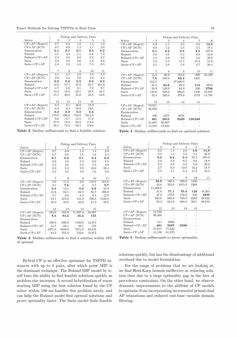
Exact Methods for Solving TSPPDs in Real Time 19
Pickup and Delivery PairsSolver 2 3 4 5 6CP+AP (Regret) 0.7 0.8 1.0 1.4 1.9CP+AP (SCN) 0.7 0.9 1.3 1.7 2.0Enumeration 0.1 0.1 0.1 0.2 0.2Ruland 2.1 3.8 5.1 6.0 7.9Ruland+CP+AP 2.3 2.6 3.0 3.2 3.7Sarin 2.0 2.6 3.6 5.8 8.6Sarin+CP+AP 2.4 3.2 4.8 7.3 9.5
7 8 9 10 11CP+AP (Regret) 2.1 2.7 3.0 4.5 5.3CP+AP (SCN) 2.6 3.3 3.6 4.6 6.4Enumeration 0.2 0.2 0.2 0.2 0.2Ruland 12.8 57.7 47.9 85.7 257.0Ruland+CP+AP 4.7 5.6 6.1 7.2 8.7Sarin 13.2 16.0 22.1 33.5 44.7Sarin+CP+AP 15.1 20.0 24.8 33.6 43.6
12 13 14 15CP+AP (Regret) 6.3 8.1 10.8 13.3CP+AP (SCN) 6.3 9.4 10.8 13.5Enumeration 0.3 0.3 0.3 0.3Ruland 172.0 396.0 752.0 7611.0Ruland+CP+AP 9.6 12.7 14.5 17.2Sarin 57.8 74.0 93.9 114.0Sarin+CP+AP 56.1 73.3 94.5 119.0
Table 2 Median milliseconds to find a feasible solution.
Pickup and Delivery PairsSolver 2 3 4 5 6CP+AP (Regret) 0.7 0.9 1.3 1.4 2.8CP+AP (SCN) 0.7 0.9 1.5 1.8 2.4Enumeration 0.1 0.2 0.1 0.2 0.2Ruland 2.6 3.8 5.2 6.0 8.5Ruland+CP+AP 2.3 2.6 3.2 3.3 3.9Sarin 2.3 5.2 9.9 16.6 33.4Sarin+CP+AP 2.4 3.5 4.9 7.6 9.8
7 8 9 10 11CP+AP (Regret) 3.0 11.2 8.9 119.0 314.0CP+AP (SCN) 3.1 7.6 4 5.7 9.7Enumeration 0.4 12.4 0.2 0.8 24.9Ruland 12.8 62.1 62.8 85.7 399.0Ruland+CP+AP 5.7 9.6 6.4 8.4 12.3Sarin 54.1 273.0 141.0 760.0 1538.0Sarin+CP+AP 16.3 23.2 24.9 41.3 50.4
12 13 14 15CP+AP (Regret) 384.0 253.0 11,267.0 33,697CP+AP (SCN) 8.5 84.2 45.2 155Enumeration - - - -Ruland 189.0 690.0 1100.0 12,674Ruland+CP+AP 14.7 88.1 49.1 176Sarin 2271.0 3450.0 7671.0 49,416Sarin+CP+AP 64.3 355.0 133.0 12,972
Table 3 Median milliseconds to find a solution within 10%of optimal.
Hybrid CP is an effective optimizer for TSPPD in-
stances with up to 8 pairs, after which point MIP is
the dominant technique. The Ruland MIP model by it-
self loses the ability to find feasible solutions quickly as
problem size increases. A second hybridization of warm
starting MIP using the best solution found by the CP
solver within 100 ms handles this problem nicely, and
can help the Ruland model find optimal solutions and
prove optimality faster. The Sarin model finds feasible
Pickup and Delivery PairsSolver 2 3 4 5 6CP+AP (Regret) 0.8 1.1 2.5 3.2 12.9CP+AP (SCN) 0.8 1.2 2.5 3.5 19.1Enumeration 0.1 0.2 0.5 2.5 107.0Ruland 2.6 3.9 5.4 6.0 16.0Ruland+CP+AP 2.4 2.8 3.9 5.0 20.6Sarin 2.3 5.5 11.7 27.9 51.6Sarin+CP+AP 2.5 3.9 5.8 9.7 28.4
7 8 9 10 11CP+AP (Regret) 14.5 90.6 184.0 899 34,429CP+AP (SCN) 7.5 249.0 62.2 1291 -Enumeration 312.0 - 37,020.0 - -Ruland 31.4 64.6 69.3 112 9844Ruland+CP+AP 20.9 120.0 65.9 220 2798Sarin 146.0 528.0 666.0 1530 33,507Sarin+CP+AP 32.4 292.0 379.0 2718 14,795
12 13 14 15CP+AP (Regret) 10,911 - - -CP+AP (SCN) 38,820 - - -Enumeration - - - -Ruland 498 6277 8676 -Ruland+CP+AP 461 2815 6220 129,648Sarin 21,697 36,807 - -Sarin+CP+AP 14,565 18,024 - -
Table 4 Median milliseconds to find an optimal solution.
Pickup and Delivery PairsSolver 2 3 4 5 6CP+AP (Regret) 0.9 1.4 2.6 4.8 14.9CP+AP (SCN) 0.9 1.3 3.5 5.4 28.9Enumeration 0.2 0.4 2.4 24.7 595.0Ruland 2.9 4.2 6.3 8.6 18.8Ruland+CP+AP 2.5 3.0 4.6 6.6 30.2Sarin 2.7 6.0 12.6 42.2 51.9Sarin+CP+AP 2.5 4.1 6.4 11.2 34.2
7 8 9 10 11CP+AP (Regret) 23.5 109.0 230.0 1236 -CP+AP (SCN) 43.6 353.0 1015.0 2268 -Enumeration 11,868.0 - - - -Ruland 31.8 71.1 70.4 129 10,263Ruland+CP+AP 47.0 178.0 176.0 239 4839Sarin 236.0 669.0 724.0 2283 39,822Sarin+CP+AP 59.2 641.0 804.0 3011 38,810
12 13 14 15CP+AP (Regret) 14,533 - - -CP+AP (SCN) 90,266 - - -Enumeration - - - -Ruland 511 6868 - -Ruland+CP+AP 481 5007 6598 -Sarin 31,017 77,622 - -Sarin+CP+AP 41,130 61,273 - -
Table 5 Median milliseconds to prove optimality.
solutions quickly, but has the disadvantage of additional
overhead due to model formulation.
For the range of problems that we are looking at,
we find Held-Karp bounds ineffective at reducing solu-
tion time due to a large optimality gap in the face of
precedence constraints. On the other hand, we observe
dramatic improvements to the abilities of CP models
to optimize from incorporating incremental primal-dual
AP relaxations and reduced cost-base variable domain
filtering.
20 Ryan J. O’Neil, Karla Hoffman
When TSPPD problems are small, most models are
effective for fast solution. It appears that one loses lit-
tle by choosing an algorithm that performs well on in-
stance with more than 10 pairs and using it on the
smaller ones as well. The Ruland model is the best
at finding and proving optimal solutions, but requires
the problem instances be symmetric. Difficulties attain-
ing feasibility of the Ruland model are easily overcome
through warm starting, and a sophisticated warm start
mechanism such as Hybrid CP with SCN branching can
positively impact its optimization abilities as well. For
asymmetric TSPPD instances, the Sarin model can be
effectively warm started in the same manner.
We believe these results provide further evidence
for the utility of hybrid optimization methods in solv-
ing hard combinatorial problems with side constraints,
and demonstrate their utility in real-time optimization.
These studies can be extended to incorporate additional
side constraints found in common pickup and delivery
problems, such as capacity and time windows. We ex-
pect such exploration will further demonstrate the ben-
efits of hybridization.
6 Compliance with Ethical Standards
On behalf of all authors, the corresponding author states
that there is no conflict of interest.
References
1. Aguayo, M.M., Sarin, S.C., Sherali, H.D.: Solvingthe single and multiple asymmetric traveling sales-
men problems by generating subtour elimination
constraints frominteger solutions. IISE Transac-
tions 50(1), 45–53 (2018)
2. Applegate, D.L., Bixby, R.E., Chvatal, V., Cook,
W.J.: The traveling salesman problem: a computa-
tional study. Princeton university press (2011)
3. Benchimol, P., Regin, J.C., Rousseau, L.M., Rue-
her, M., van Hoeve, W.J.: Improving the held and
karp approach with constraint programming. In:
International Conference on Integration of Arti-
ficial Intelligence (AI) and Operations Research
(OR) Techniques in Constraint Programming, pp.
40–44. Springer (2010)
4. Benchimol, P., Van Hoeve, W.J., Regin, J.C.,
Rousseau, L.M., Rueher, M.: Improved filtering for
weighted circuit constraints. Constraints 17(3),
205–233 (2012)
5. Berbeglia, G., Cordeau, J.F., Laporte, G.: A hybrid
tabu search and constraint programming algorithm
for the dynamic dial-a-ride problem. INFORMS
Journal on Computing 24(3), 343–355 (2012)
6. Berbeglia, G., Hahn, G.: Counting feasible solu-
tions of the traveling salesman problem with pick-
ups and deliveries is #P-complete. Discrete Ap-
plied Mathematics 157(11), 2541–2547 (2009)
7. Bertsimas, D., Jaillet, P., Martin, S.: Online Vehicle
Routing: The Edge of Optimization in Large-Scale
Applications (2018). Accepted for publication in
Operations Research
8. Carpaneto, G., Martello, S., Toth, P.: Algorithms
and codes for the assignment problem. Annals of
operations research 13(1), 191–223 (1988)
9. Caseau, Y., Laburthe, F.: Solving Small TSPs with
Constraints. In: ICLP, vol. 97, p. 104 (1997)
10. Dantzig, G., Fulkerson, R., Johnson, S.: Solution of
a large-scale traveling-salesman problem. Journal
of the operations research society of America 2(4),
393–410 (1954)
11. Dumas, Y., Desrosiers, J., Soumis, F.: The pickup
and delivery problem with time windows. European
journal of operational research 54(1), 7–22 (1991)
12. Dumitrescu, I., Ropke, S., Cordeau, J.F., Laporte,
G.: The traveling salesman problem with pickup
and delivery: polyhedral results and a branch-and-
cut algorithm. Mathematical Programming 121(2),
269 (2010)
13. Edmonds, J.: Optimum branchings. Journal of
Research of the National Bureau of Standards B
71(4), 233–240 (1967)
14. Fischetti, M., Toth, P.: An additive bounding pro-
cedure for the asymmetric travelling salesman prob-
lem. Mathematical Programming 53(1-3), 173–197
(1992)
15. Fisher, M.L.: The lagrangian relaxation method for
solving integer programming problems. Manage-
ment science 50(12 supplement), 1861–1871 (2004)
16. Focacci, F., Lodi, A., Milano, M.: A hybrid exact
algorithm for the TSPTW. INFORMS Journal on
Computing 14(4), 403–417 (2002)
17. Focacci, F., Lodi, A., Milano, M., Vigo, D.: Solving
TSP through the integration of OR and CP tech-
niques. Electronic notes in discrete mathematics 1,
13–25 (1999)
18. Gabow, H.N., Galil, Z., Spencer, T., Tarjan, R.E.:
Efficient algorithms for finding minimum spanning
trees in undirected and directed graphs. Combina-
torica 6(2), 109–122 (1986)
19. Gecode Team: Gecode: Generic constraint devel-
opment environment (2006). URL http://www.
gecode.org
20. Grubhub: TSPPD Test Instance Library. https:
//github.com/grubhub/tsppdlib (2018)
Exact Methods for Solving TSPPDs in Real Time 21
21. Gurobi Optimization, Inc.: Gurobi optimizer ref-
erence manual (2016). URL http://www.gurobi.
com
22. Held, M., Karp, R.M.: The traveling-salesman
problem and minimum spanning trees. Operations
Research 18(6), 1138–1162 (1970)
23. Held, M., Karp, R.M.: The traveling-salesman
problem and minimum spanning trees: Part ii.
Mathematical programming 1(1), 6–25 (1971)
24. Lauriere, J.L.: A language and a program for stat-
ing and solving combinatorial problems. Artificial
intelligence 10(1), 29–127 (1978)
25. Law, Y., Lee, J.: Global constraints for integer
and set value precedence. Principles and Practice
of Constraint Programming–CP 2004 pp. 362–376
(2004)
26. Lin, S.: Computer solutions of the traveling sales-
man problem. The Bell System Technical Journal
44(10), 2245–2269 (1965)
27. Lin, S., Kernighan, B.W.: An effective heuristic al-
gorithm for the traveling-salesman problem. Oper-
ations research 21(2), 498–516 (1973)
28. van Lon, R.R., Ferrante, E., Turgut, A.E., Wense-
leers, T., Berghe, G.V., Holvoet, T.: Measures of
dynamism and urgency in logistics. European Jour-
nal of Operational Research 253(3), 614–624 (2016)
29. Maher, S.J., Fischer, T., Gally, T., Gamrath, G.,
Gleixner, A., Gottwald, R.L., Hendel, G., Koch,
T., Lubbecke, M.E., Miltenberger, M., Muller, B.,
Pfetsch, M.E., Puchert, C., Rehfeldt, D., Schenker,
S., Schwarz, R., Serrano, F., Shinano, Y., Weninger,
D., Witt, J.T., Witzig, J.: The scip optimization
suite 4.0. Tech. Rep. 17-12, ZIB, Takustr.7, 14195
Berlin (2017)
30. Milano, M., Ottosson, G., Refalo, P., Thorsteins-
son, E.S.: Global constraints: When constraint pro-
gramming meets operation research. In: INFORMS
Journal on Computing, Special Issue on the Merg-
ing of Mathematical Programming and Constraint
Programming. Citeseer (2001)
31. Miller, C.E., Tucker, A.W., Zemlin, R.A.: Inte-
ger programming formulation of traveling salesman
problems. Journal of the ACM 7(4), 326–329 (1960)
32. O’Neil, R.J.: TSPPD Hybrid Optimization Code.
https://github.com/ryanjoneil/tsppd-hybrid
(2018)
33. Padberg, M., Rinaldi, G.: A branch-and-cut algo-
rithm for the resolution of large-scale symmetric
traveling salesman problems. SIAM review 33(1),
60–100 (1991)
34. Papadimitriou, C.H.: The Euclidean travelling
salesman problem is NP-complete. Theoretical
computer science 4(3), 237–244 (1977)
35. Pesant, G., Gendreau, M., Potvin, J.Y., Rousseau,
J.M.: An exact constraint logic programming al-
gorithm for the traveling salesman problem with
time windows. Transportation Science 32(1), 12–
29 (1998)
36. Pferschy, U., Stanek, R.: Generating subtour elim-
ination constraints for the TSP from pure integer
solutions. Central European Journal of Operations
Research pp. 1–30 (2016)
37. Psaraftis, H.N.: A dynamic programming solution
to the single vehicle many-to-many immediate re-
quest dial-a-ride problem. Transportation Science
14(2), 130–154 (1980)
38. Ruland, K., Rodin, E.: The pickup and de-
livery problem: Faces and branch-and-cut algo-
rithm. Computers & mathematics with applica-
tions 33(12), 1–13 (1997)
39. Sarin, S.C., Sherali, H.D., Bhootra, A.: New tighter
polynomial length formulations for the asymmet-
ric traveling salesman problem with and without
precedence constraints. Operations research letters
33(1), 62–70 (2005)
40. Valenzuela, C.L., Jones, A.J.: Estimating the held-
karp lower bound for the geometric tsp. Euro-
pean journal of operational research 102(1), 157–
175 (1997)
41. Wickham, H.: ggplot2: Elegant Graphics for Data
Analysis. Springer-Verlag New York (2009). URL
http://ggplot2.org
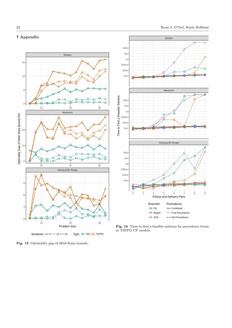
22 Ryan J. O’Neil, Karla Hoffman
7 Appendix
●●●
●
●●
●
●●
●
●●
●
●●
●
●
●
●
●
●
●
●●
●
●●
●
●●
●
●
●
●
●
●
●
●
●
●
●
●
●
●●
●●●
●
●●
●
●●
●
●
●
●
●
●
●
●●
●
●
●
●
●
●
●
●
●
●
●
●
●
●●
●
●
●
●
●●
●
●●
●
●●
●
●●
●
●●
●
●●
●
●●
●
●
●
●
●
●
●
●
●
●
●
●
●
●●
●
●●
●
●
●
●●●
Interquartile Range
Maximum
Median
10 20 30
10 20 30
10 20 30
0
5
10
15
0
10
20
0
3
6
9
Problem Size
Opt
imal
ity G
ap o
f Hel
d−K
arp
Bou
nd (
%)
Iterations 5 10 25 Type ● TSP TSPPD
Fig. 15 Optimality gap of Held-Karp bounds.
●● ● ● ● ● ● ●
● ● ●●
● ●
●●
● ● ● ● ● ● ● ●
● ● ●● ● ● ● ●
● ●●
●●
●● ●
●● ● ● ● ●
●●
●
●
●
● ● ● ●●
●
● ●
●
●
●
●
●
● ●●
● ●●
● ●
Interquartile Range
Maximum
Median
2 3 4 5 6 7 8 9
1ms
10ms
100ms
1s
10s
100s
1ms
10ms
100ms
1s
10s
100s
1ms
10ms
100ms
1s
10s
100s
Pickup and Delivery Pairs
Tim
e to
Fin
d a
Fea
sibl
e S
olut
ion
Brancher● CN
Regret
SCN
Precedence
Combined
Cost Precedence
Set Precedence
Fig. 16 Time to find a feasible solution for precedence formsin TSPPD CP models.
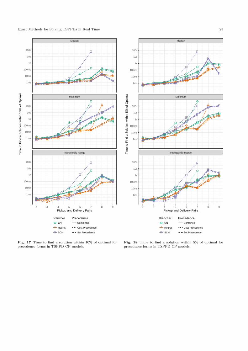
Exact Methods for Solving TSPPDs in Real Time 23
●● ●
●●
●
●●
● ● ●●
●
●
● ● ● ● ●●
●●
● ●●
●●
●
●
●
●●
●
●●
●
●●
●●
●
●
●
●
●●
●●
●
●
●
●
●●
●
●
●
●
● ●
●●
●
●
●
●
Interquartile Range
Maximum
Median
2 3 4 5 6 7 8 9
1ms
10ms
100ms
1s
10s
100s
1ms
10ms
100ms
1s
10s
100s
1ms
10ms
100ms
1s
10s
100s
Pickup and Delivery Pairs
Tim
e to
Fin
d a
Sol
utio
n w
ithin
10%
of O
ptim
al
Brancher● CN
Regret
SCN
Precedence
Combined
Cost Precedence
Set Precedence
Fig. 17 Time to find a solution within 10% of optimal forprecedence forms in TSPPD CP models.
●● ●
●
●
●
●●
● ● ●
●
●
●
●● ●
●●
●
●●
●●
●
●●
●
●●
●●
●
●●
●
● ●
●●
●
●
●●
● ●
●
●●
●
● ●
● ●
●
● ●
●
● ●
●
●●
●
● ●
Interquartile Range
Maximum
Median
2 3 4 5 6 7 8 9
1ms
10ms
100ms
1s
10s
100s
1ms
10ms
100ms
1s
10s
100s
1ms
10ms
100ms
1s
10s
100s
Pickup and Delivery Pairs
Tim
e to
Fin
d a
Sol
utio
n w
ithin
5%
of O
ptim
al
Brancher● CN
Regret
SCN
Precedence
Combined
Cost Precedence
Set Precedence
Fig. 18 Time to find a solution within 5% of optimal forprecedence forms in TSPPD CP models.
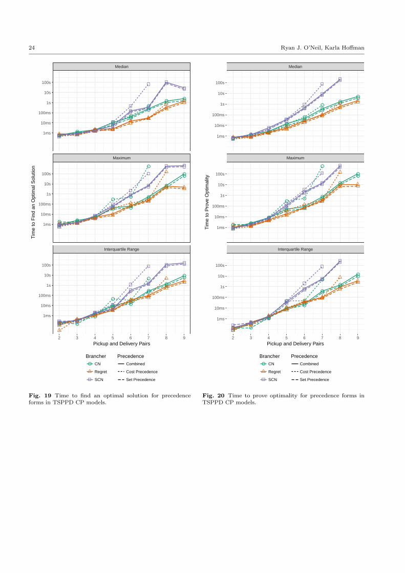
24 Ryan J. O’Neil, Karla Hoffman
●●
●
●
●
●
●●
●●
●
●
●
●
●●
●
●
●
●
●●
●●
●
● ●
●
●
●
●●
●
●●
●
● ●
●
● ●
●
●
●
●●
●
●●
●
●
●
●●
●
● ●
●
● ●
●
●●
●
●
●
Interquartile Range
Maximum
Median
2 3 4 5 6 7 8 9
1ms
10ms
100ms
1s
10s
100s
1ms
10ms
100ms
1s
10s
100s
1ms
10ms
100ms
1s
10s
100s
Pickup and Delivery Pairs
Tim
e to
Fin
d an
Opt
imal
Sol
utio
n
Brancher● CN
Regret
SCN
Precedence
Combined
Cost Precedence
Set Precedence
Fig. 19 Time to find an optimal solution for precedenceforms in TSPPD CP models.
●●
●
●
●
●
●
●
●●
●
●
●
●
●●
●
●
●
●
●
●
●●
●
●●
●
●
●
●
●
●
●●
●
● ●
●
●●
●
●
●
●
●
●
●●
●
●
●
●●
●
● ●
●
● ●
●
●●
●
●
●
Interquartile Range
Maximum
Median
2 3 4 5 6 7 8 9
1ms
10ms
100ms
1s
10s
100s
1ms
10ms
100ms
1s
10s
100s
1ms
10ms
100ms
1s
10s
100s
Pickup and Delivery Pairs
Tim
e to
Pro
ve O
ptim
ality
Brancher● CN
Regret
SCN
Precedence
Combined
Cost Precedence
Set Precedence
Fig. 20 Time to prove optimality for precedence forms inTSPPD CP models.
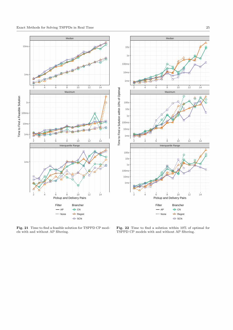
Exact Methods for Solving TSPPDs in Real Time 25
●●
●
●
●●
●●
●
●●
● ●
●
●●
●●
●● ●
●●
●●
● ●
●
●●
●●
● ●● ● ●
●●
●
●●
●● ● ●
●●
●
● ● ● ●
●
●●
●
●
●
● ●●
●
●●
●
●
●
●●
● ●
●
● ●
●
●●
●
●
●
● ● ●
Interquartile Range
Maximum
Median
2 4 6 8 10 12 14
2 4 6 8 10 12 14
2 4 6 8 10 12 14
1ms
10ms
1ms
10ms
100ms
1s
1ms
Pickup and Delivery Pairs
Tim
e to
Fin
d a
Fea
sibl
e S
olut
ion
Filter
AP
None
Brancher● CN
Regret
SCN
Fig. 21 Time to find a feasible solution for TSPPD CP mod-els with and without AP filtering.
●●
●●
●●
● ●
●
●
●
●●
●
●●
●● ●
●
●
●
●
●
●
●
● ●
● ●
●●
●
●
●
●
●
●
●
●
●●
●●
●
●
●
●
●
●● ●
●●
●●
●
●
●●
●
●
●●
●
●
● ●
●●
●
●
●
●
●
●
●
●
Interquartile Range
Maximum
Median
2 4 6 8 10 12 14
2 4 6 8 10 12 14
2 4 6 8 10 12 14
1ms
10ms
100ms
1s
10s
1ms
10ms
100ms
1s
10s
100s
1ms
10ms
100ms
1s
10s
100s
Pickup and Delivery Pairs
Tim
e to
Fin
d a
Sol
utio
n w
ithin
10%
of O
ptim
al
Filter
AP
None
Brancher● CN
Regret
SCN
Fig. 22 Time to find a solution within 10% of optimal forTSPPD CP models with and without AP filtering.
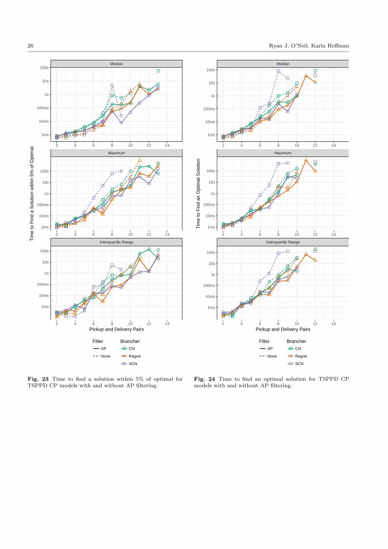
26 Ryan J. O’Neil, Karla Hoffman
●● ●
●●
●
● ● ●
●●
●
●●
●
●
●
●
●●
●
●
● ●
●●
●
●
●●
●
● ●
●
●●
●●
●
●
●
●
●
●
● ●
●
●●
●
●● ●
●
●
●
● ●
●
●
●
●
● ●
●
●
Interquartile Range
Maximum
Median
2 4 6 8 10 12 14
2 4 6 8 10 12 14
2 4 6 8 10 12 14
1ms
10ms
100ms
1s
10s
100s
1ms
10ms
100ms
1s
10s
100s
1ms
10ms
100ms
1s
10s
100s
Pickup and Delivery Pairs
Tim
e to
Fin
d a
Sol
utio
n w
ithin
5%
of O
ptim
al
Filter
AP
None
Brancher● CN
Regret
SCN
Fig. 23 Time to find a solution within 5% of optimal forTSPPD CP models with and without AP filtering.
●●
●
●
●
●
● ●
●
●
●●
●
●
●
●
●●
●
● ●
●
● ●
●
●
●●
●
● ●
●
● ●
●
●
●
●
● ●
●●
●
●
●
●●
●
●●
●
●●
●
●
●
●
Interquartile Range
Maximum
Median
2 4 6 8 10 12 14
2 4 6 8 10 12 14
2 4 6 8 10 12 14
1ms
10ms
100ms
1s
10s
100s
1ms
10ms
100ms
1s
10s
100s
1ms
10ms
100ms
1s
10s
100s
Pickup and Delivery Pairs
Tim
e to
Fin
d an
Opt
imal
Sol
utio
n
Filter
AP
None
Brancher● CN
Regret
SCN
Fig. 24 Time to find an optimal solution for TSPPD CPmodels with and without AP filtering.
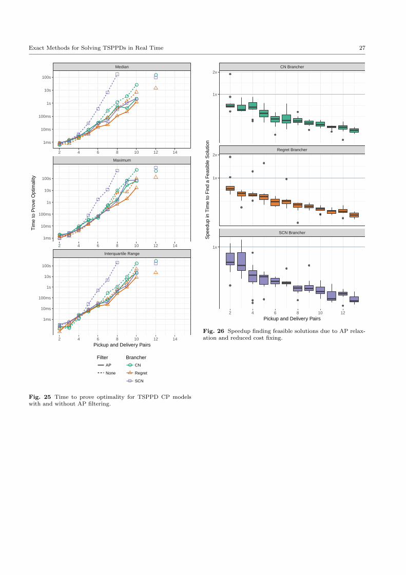
Exact Methods for Solving TSPPDs in Real Time 27
●●
●
●
●
●
●●
●
●
●●
●
●
●
●
●
●
●
● ●
●
●●
●
●
●●
●
● ●
●
●●
●
●
●
●
● ●
●●
●
●
●
●
●
●
● ●
●
●●
●
●
●
●
Interquartile Range
Maximum
Median
2 4 6 8 10 12 14
2 4 6 8 10 12 14
2 4 6 8 10 12 14
1ms
10ms
100ms
1s
10s
100s
1ms
10ms
100ms
1s
10s
100s
1ms
10ms
100ms
1s
10s
100s
Pickup and Delivery Pairs
Tim
e to
Pro
ve O
ptim
ality
Filter
AP
None
Brancher● CN
Regret
SCN
Fig. 25 Time to prove optimality for TSPPD CP modelswith and without AP filtering.
SCN Brancher
Regret Brancher
CN Brancher
2 4 6 8 10 12
1x
2x
1x
2x
1x
Pickup and Delivery Pairs
Spe
edup
in T
ime
to F
ind
a F
easi
ble
Sol
utio
n
Fig. 26 Speedup finding feasible solutions due to AP relax-ation and reduced cost fixing.
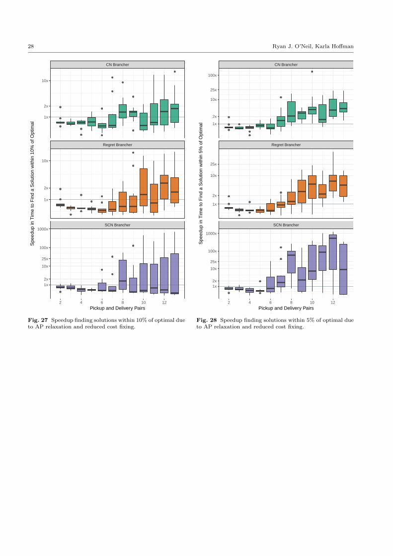
28 Ryan J. O’Neil, Karla Hoffman
SCN Brancher
Regret Brancher
CN Brancher
2 4 6 8 10 12
1x
2x
10x
1x
2x
10x
1x2x
10x
25x
100x
1000x
Pickup and Delivery Pairs
Spe
edup
in T
ime
to F
ind
a S
olut
ion
with
in 1
0% o
f Opt
imal
Fig. 27 Speedup finding solutions within 10% of optimal dueto AP relaxation and reduced cost fixing.
SCN Brancher
Regret Brancher
CN Brancher
2 4 6 8 10 12
1x
2x
10x
25x
100x
1x
2x
10x
25x
1x2x
10x
25x
100x
1000x
Pickup and Delivery Pairs
Spe
edup
in T
ime
to F
ind
a S
olut
ion
with
in 5
% o
f Opt
imal
Fig. 28 Speedup finding solutions within 5% of optimal dueto AP relaxation and reduced cost fixing.
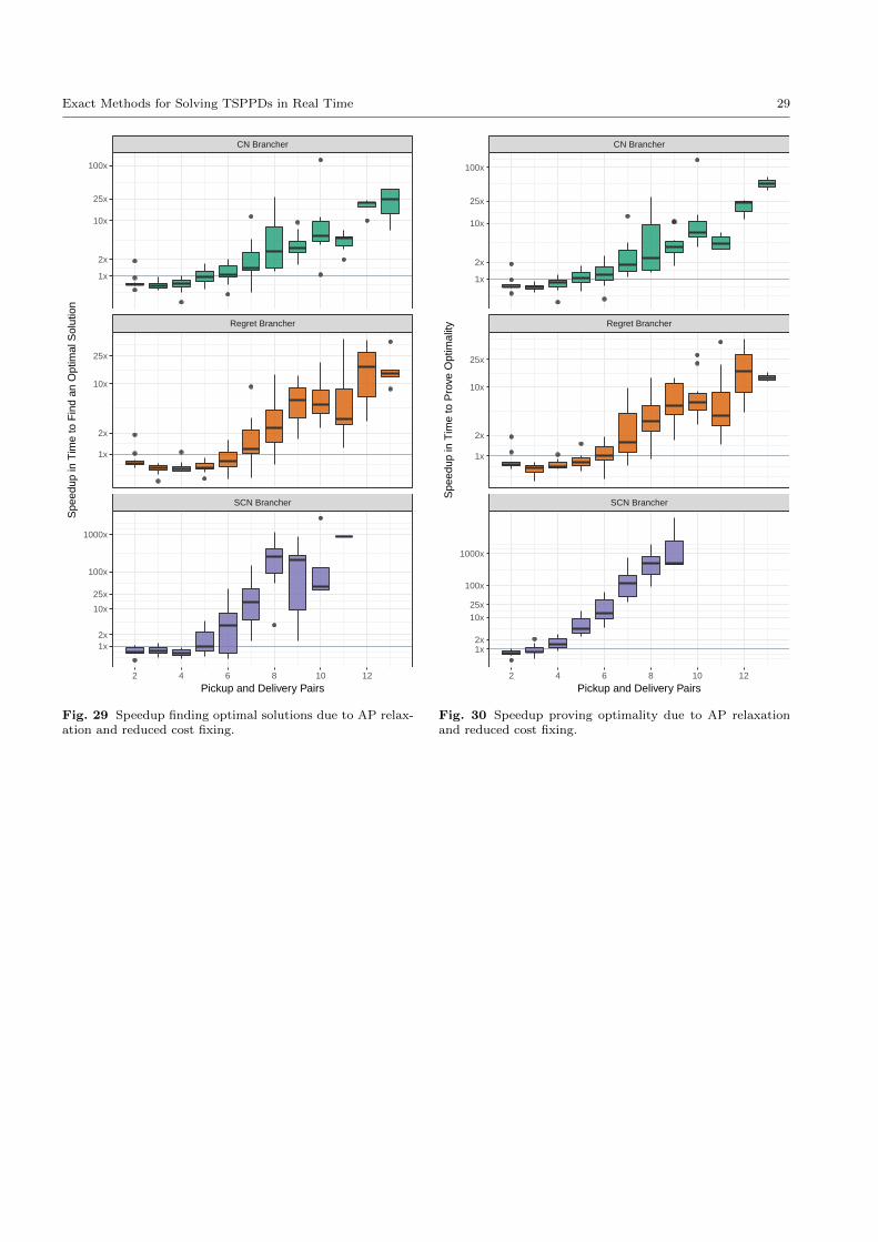
Exact Methods for Solving TSPPDs in Real Time 29
SCN Brancher
Regret Brancher
CN Brancher
2 4 6 8 10 12
1x
2x
10x
25x
100x
1x
2x
10x
25x
1x2x
10x
25x
100x
1000x
Pickup and Delivery Pairs
Spe
edup
in T
ime
to F
ind
an O
ptim
al S
olut
ion
Fig. 29 Speedup finding optimal solutions due to AP relax-ation and reduced cost fixing.
SCN Brancher
Regret Brancher
CN Brancher
2 4 6 8 10 12
1x
2x
10x
25x
100x
1x
2x
10x
25x
1x2x
10x25x
100x
1000x
Pickup and Delivery Pairs
Spe
edup
in T
ime
to P
rove
Opt
imal
ity
Fig. 30 Speedup proving optimality due to AP relaxationand reduced cost fixing.
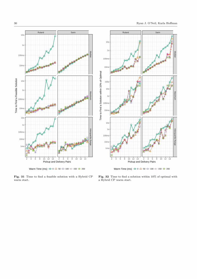
30 Ryan J. O’Neil, Karla Hoffman
●
●● ●
●●
● ●
●
●●
●
●
●
●
●●
●
●
●
●●
●
●
●
●
●●
●
●●
●●
●●
●●
●●
● ●
●
●●
●●
●● ●
●●
●●
●● ●
●
●●
●●
● ●●
● ●●
●
● ●
●
● ●
●
● ●
●●
● ● ●●
● ●
Ruland Sarin
Median
Maxim
umInterquartile R
ange
2 4 6 8 10 12 14 2 4 6 8 10 12 14
10ms
100ms
1s
10s
10ms
100ms
1s
10s
1ms
10ms
100ms
1s
10s
Pickup and Delivery Pairs
Tim
e to
Fin
d a
Fea
sibl
e S
olut
ion
Warm Time (ms) ● 0 50 100 150 200
Fig. 31 Time to find a feasible solution with a Hybrid CPwarm start.
●●
● ●●
●
● ●●
●
●
●●
●
●●
●●
●●
●
●●
●●
●
●●
●
●●
● ●
●
●●
●
●
●
●●
●
●
●
●●
●●
●
●
●
●●
●
●
●
●
● ●
● ●
●
● ●
●
●
●
●
●
●
●● ●
● ● ●
● ●
● ●● ●
●
●
Ruland Sarin
Median
Maxim
umInterquartile R
ange
2 4 6 8 10 12 14 2 4 6 8 10 12 14
10ms
100ms
1s
10s
10ms
100ms
1s
10s
100s
1ms
10ms
100ms
1s
10s
Pickup and Delivery Pairs
Tim
e to
Fin
d a
Sol
utio
n w
ithin
10%
of O
ptim
al
Warm Time (ms) ● 0 50 100 150 200
Fig. 32 Time to find a solution within 10% of optimal witha Hybrid CP warm start.
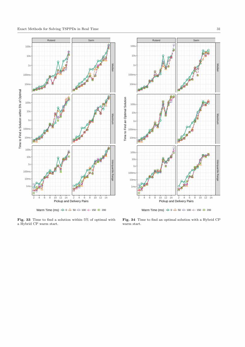
Exact Methods for Solving TSPPDs in Real Time 31
●●
● ●●
●
● ●●
●
●
●●
●
●●
●●
● ●
●
●
●
●
●
●
●
●
●
● ●
●●
●
●●
●
●
●
●●
●
●
●
●●
●●
● ●
●
● ●
●
●
●
●
● ●
● ●
●
●●
●
●●
●
●
●
●●
●
● ●
● ●
●
● ●● ●
●
●
Ruland Sarin
Median
Maxim
umInterquartile R
ange
2 4 6 8 10 12 14 2 4 6 8 10 12 14
10ms
100ms
1s
10s
100s
10ms
100ms
1s
10s
100s
1ms
10ms
100ms
1s
10s
100s
Pickup and Delivery Pairs
Tim
e to
Fin
d a
Sol
utio
n w
ithin
5%
of O
ptim
al
Warm Time (ms) ● 0 50 100 150 200
Fig. 33 Time to find a solution within 5% of optimal witha Hybrid CP warm start.
●●
● ●
●
●
● ●●
●
●
●●
●●
●●
● ●
●
●
●
●
●
●
●
●
● ●
●●
●●
●●
●
●
●●
●
●
●
●●
●
● ●
●
●●
●
●
●●
● ●
●
●
●
●
●● ●
●
●●
●
●
● ●●
●
● ● ●
Ruland Sarin
Median
Maxim
umInterquartile R
ange
2 4 6 8 10 12 14 2 4 6 8 10 12 14
10ms
100ms
1s
10s
100s
10ms
100ms
1s
10s
100s
1ms
10ms
100ms
1s
10s
100s
Pickup and Delivery Pairs
Tim
e to
Fin
d an
Opt
imal
Sol
utio
n
Warm Time (ms) ● 0 50 100 150 200
Fig. 34 Time to find an optimal solution with a Hybrid CPwarm start.
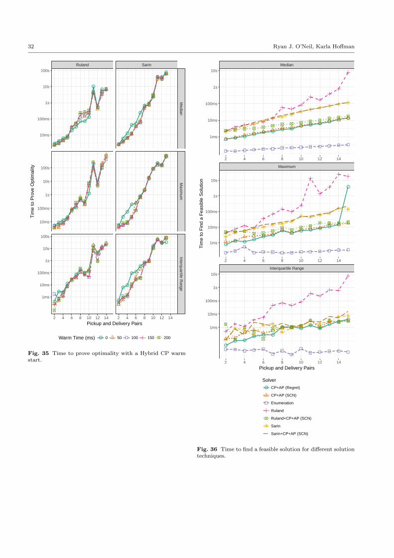
32 Ryan J. O’Neil, Karla Hoffman
●●
●●
●●
● ●●
●
●
●
●●
●●
●●
●
●
●
●
●
●
●
● ●
●●
●
●●
●
●
●
●
●
●
●
● ●
●
● ●
●
● ●
●
●
●
●
● ●
●
●
●
●
● ●
●
●
●●
● ●
●● ●
●
●● ●
Ruland Sarin
Median
Maxim
umInterquartile R
ange
2 4 6 8 10 12 14 2 4 6 8 10 12 14
10ms
100ms
1s
10s
100s
10ms
100ms
1s
10s
100s
1ms
10ms
100ms
1s
10s
100s
Pickup and Delivery Pairs
Tim
e to
Pro
ve O
ptim
ality
Warm Time (ms) ● 0 50 100 150 200
Fig. 35 Time to prove optimality with a Hybrid CP warmstart.
● ● ●●
● ●● ●
● ● ●●
● ●
●● ●
●● ●
●●
● ● ● ●●
●
●● ●
● ● ●
● ● ●●
●●
●●
Interquartile Range
Maximum
Median
2 4 6 8 10 12 14
2 4 6 8 10 12 14
2 4 6 8 10 12 14
1ms
10ms
100ms
1s
10s
1ms
10ms
100ms
1s
10s
1ms
10ms
100ms
1s
10s
Pickup and Delivery Pairs
Tim
e to
Fin
d a
Fea
sibl
e S
olut
ion
Solver● CP+AP (Regret)
CP+AP (SCN)
Enumeration
Ruland
Ruland+CP+AP (SCN)
Sarin
Sarin+CP+AP (SCN)
Fig. 36 Time to find a feasible solution for different solutiontechniques.
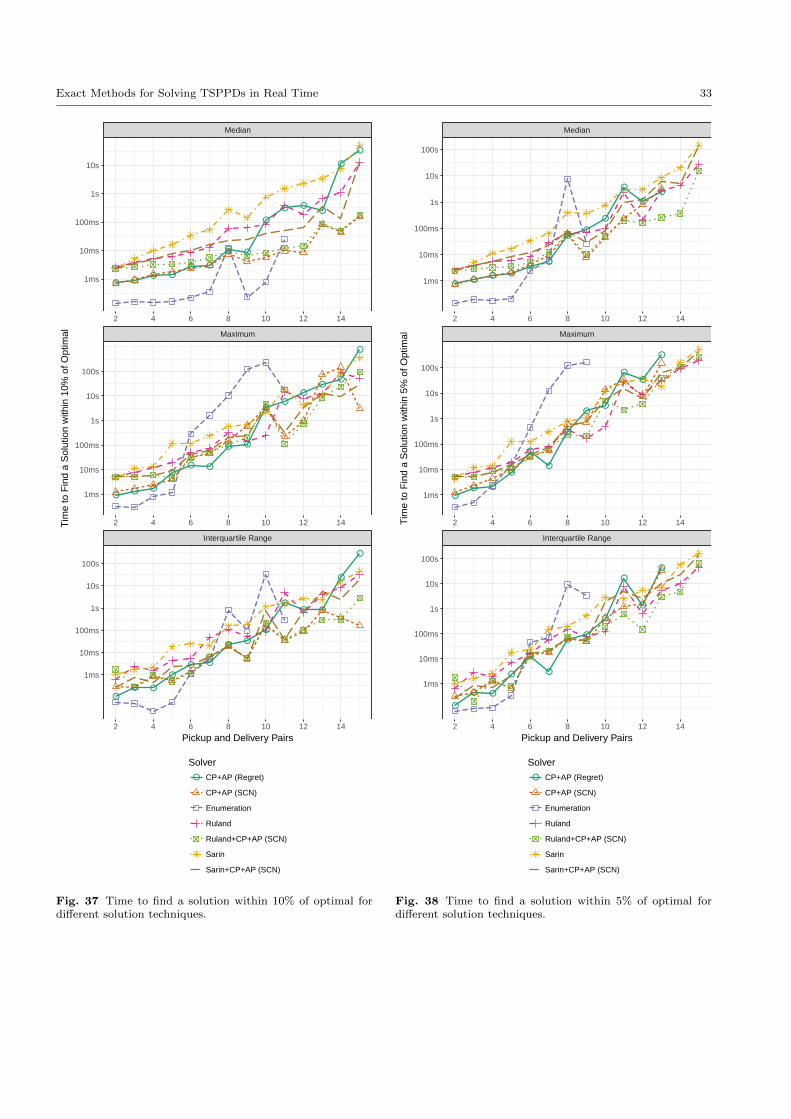
Exact Methods for Solving TSPPDs in Real Time 33
● ●● ●
● ●
● ●
●
● ●●
●
●
●● ●
●● ●
● ●
●●
●●
●
●
●● ●
●
● ●
●●
●
●● ●
●
●
Interquartile Range
Maximum
Median
2 4 6 8 10 12 14
2 4 6 8 10 12 14
2 4 6 8 10 12 14
1ms
10ms
100ms
1s
10s
1ms
10ms
100ms
1s
10s
100s
1ms
10ms
100ms
1s
10s
100s
Pickup and Delivery Pairs
Tim
e to
Fin
d a
Sol
utio
n w
ithin
10%
of O
ptim
al
Solver● CP+AP (Regret)
CP+AP (SCN)
Enumeration
Ruland
Ruland+CP+AP (SCN)
Sarin
Sarin+CP+AP (SCN)
Fig. 37 Time to find a solution within 10% of optimal fordifferent solution techniques.
●●
● ●●
●
●●
●
●
●
●
●● ●
●
●
●
●
●●
●●
●
●
● ●
●
●
●
●●
●
●
●
●
Interquartile Range
Maximum
Median
2 4 6 8 10 12 14
2 4 6 8 10 12 14
2 4 6 8 10 12 14
1ms
10ms
100ms
1s
10s
100s
1ms
10ms
100ms
1s
10s
100s
1ms
10ms
100ms
1s
10s
100s
Pickup and Delivery Pairs
Tim
e to
Fin
d a
Sol
utio
n w
ithin
5%
of O
ptim
al
Solver● CP+AP (Regret)
CP+AP (SCN)
Enumeration
Ruland
Ruland+CP+AP (SCN)
Sarin
Sarin+CP+AP (SCN)
Fig. 38 Time to find a solution within 5% of optimal fordifferent solution techniques.
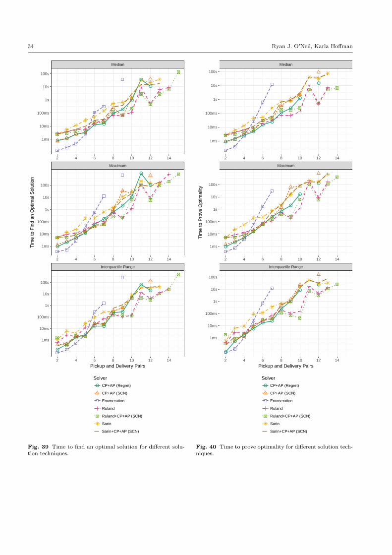
34 Ryan J. O’Neil, Karla Hoffman
●●
● ●
● ●
●●
●
●
●
●●
●
●
●
●
●
●
●
●
●
●
●
●●
● ●
● ●
●
●
●
Interquartile Range
Maximum
Median
2 4 6 8 10 12 14
2 4 6 8 10 12 14
2 4 6 8 10 12 14
1ms
10ms
100ms
1s
10s
100s
1ms
10ms
100ms
1s
10s
100s
1ms
10ms
100ms
1s
10s
100s
Pickup and Delivery Pairs
Tim
e to
Fin
d an
Opt
imal
Sol
utio
n
Solver● CP+AP (Regret)
CP+AP (SCN)
Enumeration
Ruland
Ruland+CP+AP (SCN)
Sarin
Sarin+CP+AP (SCN)
Fig. 39 Time to find an optimal solution for different solu-tion techniques.
●●
●●
●●
●
●
●
●
●●
●
●
●
●
●
●
●
●
●
●
●
●
● ●
●
●
●
●
Interquartile Range
Maximum
Median
2 4 6 8 10 12 14
2 4 6 8 10 12 14
2 4 6 8 10 12 14
1ms
10ms
100ms
1s
10s
100s
1ms
10ms
100ms
1s
10s
100s
1ms
10ms
100ms
1s
10s
100s
Pickup and Delivery Pairs
Tim
e to
Pro
ve O
ptim
ality
Solver● CP+AP (Regret)
CP+AP (SCN)
Enumeration
Ruland
Ruland+CP+AP (SCN)
Sarin
Sarin+CP+AP (SCN)
Fig. 40 Time to prove optimality for different solution tech-niques.