exam schools, ability, and the effects of affirmative

Columbia University

Department of Economics

Discussion Paper Series

Exam Schools, Ability, and the Effects of Affirmative Action:

Latent Factor Extrapolation in the Regression Discontinuity

Design

Miikka Rokkaneny

Discussion Paper No.: 1415-03

Department of Economics

Columbia University

New York, NY 10027

March 2015

Exam Schools, Ability, and the Effects of Affirmative Action:

Latent Factor Extrapolation in the Regression Discontinuity Design∗

Miikka Rokkanen†

March 26, 2015

Abstract

Selective school admissions give rise to a Regression Discontinuity (RD) design that non-

parametrically identifies causal effects for marginal applicants. Without stronger assumptions

nothing can be said about causal effects for inframarginal applicants. Estimates of causal effects

for inframarginal applicants are valuable for many policy questions, such as affirmative action,

that substantially alter admissions cutoffs. This paper develops a latent factor-based approach

to RD extrapolation that is then used to estimate effects of Boston exam schools away from

admissions cutoffs. Achievement gains from Boston exam schools are larger for applicants with

lower English and Math abilities. I also use the model to predict the effects of introducing

either minority or socioeconomic preferences in exam school admissions. Affirmative action has

modest average effects on achievement, while increasing the achievement of the applicants who

gain access to exam schools as a result.

Keywords: Affirmative Action, Extrapolation, Latent Factor, Regression Discontinuity Design,

Selective School

∗I would like to thank Isaiah Andrews, Joshua Angrist, David Autor, Alex Bartik, Erich Battistin, Stephane Bon-homme, Victor Chernozhukov, Clement de Chaisemartin, Yingying Dong, Kirill Evdokimov, Benjamin Feigenberg,Eliza Forsythe, Jerry Hausman, Guido Imbens, Patrick Kline, Liisa Laine, Bradley Larsen, Anna Mikusheva, ConradMiller, Yusuke Narita, Whitney Newey, Juan Passadore, Parag Pathak, Adam Sacarny, Matti Sarvimaki, AnnalisaScognamiglio, Henry Swift, Roope Uusitalo, Chris Walters and Heidi Williams as well as the seminar participantsat Boston University, Columbia University, Dartmouth College, Federal Reserve Bank of New York, Helsinki Centerof Economic Research, INSEAD, Institute for International Economic Studies, London School of Economics, Mas-sachusetts Institute of Technology, Michigan State University, Norwegian School of Economics, Teachers College, UCSan Diego, University of Warwick, University of Western Ontario, and Uppsala University for their helpful commentsand suggestions. I would also like to thank Kamal Chavda and the Boston Public Schools for graciously sharing data.†Columbia University, Department of Economics, 420 West 118th Street, New York, NY 10027. Email:

[email protected].

1

1 Introduction

Regression Discontinuity (RD) methods identify treatment effects for individuals at the cutoff

value determining treatment assignment under relatively mild assumptions. Without stronger

assumptions, however, nothing can be said about treatment effects for individuals away from the

cutoff. Such effects may be valuable for predicting the effects of policies that change treatment

assignments of a broader group. An important example of this are affirmative action policies that

change cutoffs substantially.

Motivated by affirmative action considerations, this paper develops a strategy for the identifica-

tion and estimation of causal effects for inframarginal applicants to Boston’s selective high schools,

known as exam schools. The exam schools, spanning grades 7-12, are seen as the flagship of the

Boston Public Schools (BPS) system. They offer higher-achieving peers and an advanced curricu-

lum. Admissions to these schools are based on Grade Point Average (GPA) and the Independent

School Entrance Exam (ISEE). The RD design generated by exam school admissions nonparamet-

rically identifies causal effects of exam school attendance for marginal applicants at admissions

cutoffs. Abdulkadiroglu, Angrist, and Pathak (2014) use this strategy and find little evidence of

effects for these applicants.1 Other applicants, however, may benefit or suffer as a consequence of

exam school attendance.

Treatment effects away from RD cutoffs are especially important for discussions of affirmative

action at exam schools. Boston exam schools have played an important role in the history of

attempts to ameliorate racial imbalances in Boston. In 1974 a federal court ruling introduced the

use of minority preferences in Boston exam school admissions as part of a city-wide desegregation

plan. Court challenges later led Boston to drop racial preferences. Similarly, Chicago switched

from minority to socioeconomic preferences in exam school admissions following a federal court

ruling in 2009.2

This paper develops a latent factor-based approach to the identification and estimation of

treatment effects away from the cutoff. I assume that the source of omitted variables bias in an

RD design can be modeled using latent factors. The running variable is one of a number of noisy

measures of these factors. Assuming other noisy measures are available, causal effects for all values

1Dobbie and Fryer (2014) find similar results in an RD study of New York City exam schools.2The use of affirmative action in exam school admissions is a highly contentious issue also in New York City where

a federal complaint was filed in 2012 against the purely achievement-based exam school admissions because of thedisproportionately low minority shares at these schools.

2

of the running variable are nonparametrically identified.3 In related work on the same problem,

Angrist and Rokkanen (forthcoming) postulate a strong conditional independence assumption that

identifies causal effects away from RD cutoffs. The framework developed here relies on weaker

assumptions and is likely to find wider application.4

I use this framework to estimate causal effects of exam school attendance for the full population

of applicants. These estimates suggest that the achievement gains from exam school attendance

are larger among applicants with lower baseline measures of ability. I use these estimates to

simulate effects of introducing either minority or socioeconomic preferences in Boston exam school

admissions. The reforms change the admissions cutoffs faced by different applicant groups and affect

the exam school assignment of 27-35% of applicants. The simulations suggest that the reforms boost

achievement among applicants. These effects are largely driven by achievement gains experienced

by lower-achieving applicants who gain access to exam schools as a result.

In developing the latent factor-based approach to RD extrapolation I build on the literatures

on measurement error models (Hu and Schennach, 2008) and nonparametric instrumental variable

models (Newey and Powell, 2003). Latent factor models have a long tradition in economics (Aigner,

Hsiao, Kapteyn, and Wansbeek, 1984). In the program evaluation literature they have been used, for

instance, to identify the joint distribution of potential outcomes (Aakvik, Heckman, and Vytlacil,

2005), time-varying treatment effects (Cooley Fruehwirth, Navarro, and Takahashi, 2014), and

distributional treatment effects (Bonhomme and Sauder, 2011).

The educational consequences of affirmative action have mostly been studied in post-secondary

schools with a focus on application and enrollment margins. Several papers have studied affirmative

action bans in California and Texas as well as the introduction of the Texas 10% plan (Long,

2004; Card and Krueger, 2005; Dickson, 2006; Andrews, Ranchhod, and Sathy, 2010; Cortes, 2010;

Antonovics and Backes, 2013, 2014). Howell (2010) uses a structural model to simulate the effects of

a nation-wide elimination of affirmative action in college admissions, and Hinrichs (2012) studies the

effects of various affirmative action bans around the United States. Only a few studies have looked

at the effects of affirmative action in selective school admissions on later outcomes (Arcidiacono,

2005; Rothstein and Yoon, 2008; Bertrand, Hanna, and Mullainathan, 2010; Francis and Tannuri-

Pianto, 2012; Kapor, 2015).

3This is similar to ideas put forth by Lee (2008), Lee and Lemieux (2010), DiNardo and Lee (2011), and Bloom(2012). However, this is the first paper that discusses how this framework can be used in RD extrapolation.

4For other approaches to RD extrapolation, see Angrist and Pischke (2009), Jackson (2010), DiNardo and Lee(2011), Wing and Cook (2013), Bargain and Doorley (2013), Bertanha and Imbens (2014), and Dong and Lewbel(forthcoming).

3

The rest of the paper is organized as follows. The next section outlines the econometric frame-

work in a sharp RD design. Section 3 discusses an extension to a fuzzy RD design. Section 4

discusses identification and estimation of the latent factor model in the Boston exam schools set-

ting. Section 5 reports the estimation results. Section 6 uses the estimates to simulate effects of

affirmative action. Section 7 concludes.

2 Latent Factor Extrapolation in a Sharp RD Design

2.1 Framework

In a sharp RD design a binary treatment D ∈ {0, 1} is a deterministic function of an observed,

continuous running variable R ∈ R and a known cutoff c:

D = 1 (R ≥ c) .

Individuals with running values less than c do not receive the treatment whereas individuals with

running variable values above c receive the treatment. Each individual is associated with two

potential outcomes: Y (0) is the outcome of an individual if she does not receive the treatment

(D = 0), and Y (1) is the outcome of an individual if she receives the treatment (D = 1). The

observed outcome of an individual is

Y = (1−D)× Y (0) +D × Y (1) .

I ignore additional covariates to simplify notation. Everything that follows can be generalized to

allow for additional covariates by conditioning on them throughout.

Sharp RD allows one to nonparametrically identify the Average Treatment Effect (ATE) at the

cutoff, E [Y (1)− Y (0) | R = c], under relatively mild conditions, listed in Assumption A. Under

these assumptions, the ATE is given by the discontinuity in E [Y | R] at the cutoff, as shown in

Lemma 1 (Hahn, Todd, and van der Klaauw, 2001).

Assumption A.

1. fR (r) > 0 in a neighborhood around c.

2. E [Y (0) | R = r] and E [Y (1) | R = r] are continuous in r at c for all y ∈ Y.

3. E [|Y (0)| | R = c] , E [|Y (1)| | R = c] <∞.

4

𝐸[𝑌(1) − 𝑌(0)| 𝑅 = 𝑐]

𝑅

𝐸[𝑌(1)|𝑅]

𝐸[𝑌(0)|𝑅]

𝑐

𝐸[𝑌(1) − 𝑌(0)| 𝑅 = 𝑟1]

𝑟1

𝐸[𝑌(0)| 𝑅 = 𝑟1]

𝐸[𝑌(1)| 𝑅 = 𝑟1]

𝐸[𝑌(1) − 𝑌(0)| 𝑅 = 𝑟0]

𝐸[𝑌(0)| 𝑅 = 𝑟0]

𝑟0

𝐸[𝑌(1)| 𝑅 = 𝑟0]

𝑌(0),𝑌(1)

Figure 1: Extrapolation Problem in a Sharp Regression Discontinuity Design

Lemma 1. (Hahn, Todd, and van der Klaauw, 2001) Suppose Assumption A holds. Then

E [Y (1)− Y (0) | R = c] = limδ↓0{E [Y | R = c+ δ]− E [Y | R = c− δ]} .

The drawback of sharp RD is that it does not allow one to say anything about the ATE away

from the cutoff, E [Y (1)− Y (0) | R = r] for r 6= c. Figure 1 illustrates this extrapolation problem.

To the left of the cutoff we observe Y (0) whereas to the right of the cutoff we observe Y (1). The

relevant counterfactual outcomes are instead unobservable. Suppose we wanted to know the ATE

at R = r0 to the left of the cutoff, E [Y (1)− Y (0) | R = r0]. We observe E [Y (0) | R = r0], but the

counterfactual E [Y (1) | R = r0] is unobservable. Similarly, suppose we wanted to know the ATE

at R = r1 to the right of the cutoff, E [Y (1)− Y (0) | R = r1]. We observe E [Y (1) | R = r1], but

the counterfactual E [Y (0) | R = r1] is unobservable. Therefore, in order to identify these ATEs,

one is forced to extrapolate from one side of the cutoff to the other.

This paper develops a latent factor-based solution to the extrapolation problem. I consider a

5

𝑅 𝜃𝑙𝑜𝑤

𝜃ℎ𝑖𝑔ℎ

𝜃𝑙𝑜𝑤 + 𝜈𝑅𝑙𝑜𝑤 𝜃𝑙𝑜𝑤 + 𝜈𝑅ℎ𝑖𝑔ℎ 𝜃ℎ𝑖𝑔ℎ + 𝜈𝑅𝑙𝑜𝑤 𝜃ℎ𝑖𝑔ℎ + 𝜈𝑅

ℎ𝑖𝑔ℎ 𝑐

Figure 2: Treatment Assignment in the Latent Factor Framework

setting in which R is a function of a latent factor θ and a disturbance νR:

R = gR (θ, νR)

where gR is an unknown function, and both θ and νR are unobservable and potentially multidi-

mensional. One example of such setting is selective school admissions where R is an entrance exam

score that can be thought of as a noisy measure of an applicant’s academic ability θ.

Figure 2 illustrates the latent factor framework when both θ and νR are scalars and R = θ+νR.

Consider two types of individuals with low and high levels of θ, θlow < c and θhigh > c. If there was

no noise in R, individuals with θ = θlow would not receive the treatment whereas individuals with

θ = θhigh would receive the treatment. However, because of the noise in R, some of the individuals

with θ = θlow end up to the right of the cutoff, and some of the individuals with θ = θhigh to the

left of the cutoff. This means that both types of individuals are observed with and without the

treatment. In the selective school admissions example this means that applicants with the same

level of academic ability end up on different sides of the admissions cutoff because of, say, having

a good or a bad day when taking the entrance exam.

I assume that the potential outcomes Y (0) and Y (1) are conditionally independent of R given

θ, as stated in Assumption B. In the selective school admissions example this means that while

Y (0) and Y (1) may depend on an applicant’s academic ability, they do not depend on the noise in

the entrance exam score. Assumption B implies that any dependence of (Y (0) , Y (1)) on R is solely

due to the dependence of (Y (0) , Y (1)) on θ and the dependence of R on θ. Lemma 2 highlights

the key implication of Assumption B: the ATE at R = r, E [Y (1)− Y (0) | R = r], depends on the

6

latent conditional ATE given θ, E [Y (1)− Y (0) | θ], and the conditional distribution of θ given

R, fθ|R. Therefore, the identification of the ATE away from the cutoff depends on one’s ability to

identify these two objects.

Assumption B. (Y (0) , Y (1)) ⊥⊥ R | θ.

Lemma 2. Suppose that Assumption B holds. Then

E [Y (1)− Y (0) | R = r] = E {E [Y (1)− Y (0) | θ] | R = r}

for all r ∈ R.

Consider again the identification of the ATE for individuals with R = r0 to the left of the cutoff

and for individuals with R = r1 to the right of the cutoff, illustrated in Figure 1. As discussed above,

the shap RD design allows one to observe E [Y (0) | R = r0] and E [Y (1) | R = r1], and the extrap-

olation problem arises from the unobservability of E [Y (1) | R = r0] and E [Y (0) | R = r1]. Sup-

pose the conditional expectation functions of Y (0) and Y (1) given θ, E [Y (0) | θ] and E [Y (1) | θ]

are known. In addition, suppose the conditional distributions of θ given R = r0 and R = r1,

fθ|R (θ | r0) and fθ|R (θ | r1), are known. Then, under Assumption B, the unobserved counterfactu-

als E [Y (1) | R = r0] and E [Y (0) | R = r1] are given by

E [Y (1) | R = r0] = E {E [Y (1) | θ] | R = r0}

E [Y (0) | R = r1] = E {E [Y (0) | θ] | R = r1} .

There is only one remaining issue: how does one identify E [Y (0) | θ], E [Y (1) | θ], and fθ|R?

If θ was observable, these objects could be identified following the covariate-based approach devel-

oped by Angrist and Rokkanen (forthcoming). However, here the unobservability of θ requires an

alternative approach. To achieve identification, I rely on the availability of multiple noisy measures

of θ. I focus on a setting where θ is one-dimensional for simplicity. Extension to a setting where θ

is multidimensional is discussed in the end of this section.

7

I assume that the data contains three noisy measures of θ, denoted by M1, M2, and M3:

M1 = gM1 (θ, νM1)

M2 = gM2 (θ, νM2)

M3 = gM3 (θ, νM3)

where gM1 , gM2 , and gM3 are unknown functions, and νM1 , νM2 , and νM3 are potentially multi-

dimensional disturbances. I require θ, M1, and M2 to be continuous but allow M3 to be either

continuous or discrete; even a binary M3 is sufficient. I denote the supports of θ, M1, M2, and

M3 by Θ, M1, M2, and M3. I will occasionally also use the notation M = (M1,M2,M3) and

M =M1 ×M2 ×M3.

I focus on a setting in which is R is a deterministic function of aa subset of M . It is possible

to allow for a more general setting where the relationship between R and M is stochastic as long

as this additional this additional noise is not related to the potential outcomes. In the selective

school admissions example, one could think of M1 as the entrance exam score and M2 and M3 as

two (pre-application) baseline test scores.

2.2 Parametric Example

To provide a benchmark for the discussion about nonparametric identification of the latent factor

model, I start by considering the identification of a simple parametric example .

The measurement model takes the following form:

M1 = θ + νMk, k = 1, 2, 3

M2 = µM2 + λM2θ + νM2

M3 = µM3 + λM3θ + νM3

where θ

νM1

νM2

νM3

∼ N

µθ

0

0

0

,σ2θ 0 0 0

0 σ2νM1

0 0

0 0 σ2νM2

0

0 0 0 σ2νM3

.

8

The intercept and slope in the first measurement equation are normalized to 0 and 1 without loss

of generality in order pin down the location and scale of θ.

The latent outcome model takes the following form:

E [Y (0) | θ] = α0 + β0θ

E [Y (1) | θ] = α1 + β1θ.

I assume that the potential outcomes Y (0) and Y (1) are conditionally independent of M given θ.

Formally,

(Y (0) , Y (1)) ⊥⊥M | θ.

This implies that the measurements are related to the potential outcomes only through θ. They

are used as instruments to identify the relationships between Y (0) and θ and Y (1) and θ.

The parameters of the measurement model can be identified from the means, variances, covari-

ances of the joint distrubution of M1, M2, and M3 by noticing that

E [M1] = µθ

E [Mk] = µMk+ λMk

µθ, k = 2, 3

V ar [M1] = σ2θ + σ2

νM1

V ar [Mk] = λ2Mkσ2θ + σ2

νMk, k = 2, 3

Cov [M2,M3] = λM2λM3σ2θ

Cov [M1,Mk] = λMkσ2θ , k = 2, 3.

This allows one to derive closed-form solutions for all of the parameters.

The parameters of the latent outcome model can be identified from the conditional expectation

of Y given M and D and the conditional expectation of θ given M and D by noticing that

E[Y |M = m0, D = 0

]= α0 + β0E

[θ |M = m0, D = 0

]E[Y |M = m1, D = 1

]= α1 + β1E

[θ |M = m1, D = 1

]for all m0 ∈M0 and m1 ∈M1 whereMd denotes the conditional support of M given D = d. This

9

allows one to identify the parameters of the latent outcome model by essentially running regressions

of Y on predicted θ (given M) using data only to the left (D = 0) or to the right (D = 1) of the

cutoff.

Finally, E [Y (0) | R = r] and E [Y (1) | R = r] and E [Y (1)− Y (0) | R = r] are given by

E [Y (0) | R = r] = α0 + β0E [θ | R = r]

E [Y (1) | R = r] = α1 + β1E [θ | R = r]

E [Y (1)− Y (0) | R = r] = (α1 − α0) + (β1 − β0)E [θ | R = r]

where E [θ | R] = E [E [θ |M ] | R] for all r ∈ R.

2.3 Nonparametric Identification

In this section I discuss nonparametric identification in the latent factor framework. I start by

discussing the identification of the measurement model that takes the form

M1 = gM1 (θ, νM1)

M2 = gM2 (θ, νM2)

M3 = gM3 (θ, νM3) .

There are several approaches available in the literature for identifying the underlying measure-

ment model from the joint distribution of noisy measurements (see, for instance, Chen, Hong, and

Nekipelov (2011) for a review). These approaches differ in how they deal with the tradeoff between

(a) how many restrictions are imposed on the measurement model and (b) how much is required

from the data. I focus on a particular approach by Hu and Schennach (2008) as it allows one to be

relatively agnostic about the measurement model.

Assumption C lists the conditions under which the masurement model is nonparametrically

identified. (Hu and Schennach, 2008; Cunha, Heckman, and Schennach, 2010).

Assumption C.

1. fθ,M (θ,m) is bounded with respect to the product measure of the Lebesgue measure on Θ ×

M1×M2 and some dominating measure µ onM3. All the corresponding marginal and conditional

densities are also bounded.

2. M1, M2, and M3 are jointly independent conditional on θ.

10

3. For all θ′, θ′′ ∈ Θ, fM3|θ

(m3 | θ

′)

and fM3|θ

(m3 | θ

′′)

differ over a set of strictly positive

probability whenever θ′ 6= θ

′′.

4. There exists a known functional H such that H[fM1|θ (· | θ)

]= θ for all θ ∈ Θ.

5. fθ|M1(θ | m1) and fM1|M2

(m1 | m2) form (boundedly) complete families of distributions indexed

by m1 ∈M1 and m2 ∈M2.

Assumption C.1 requires θ, M1, and M2 to be continuous but allows M3 to be either continuous

or discrete. It also restricts the joint, marginal and conditional densities of θ, M1, M2, and M3 to

be bounded. Assumption C.2 requires νM1 , νM2 , and νM3 to be jointly independent conditional on

θ but allows for arbitrary dependence between θ and these disturbances, such as heteroscedasticity.

Assumption C.3 requires the conditional distribution of M3 given θ to vary as a function of θ.

This assumption can be satisfied, for instance, by assuming strict monotonicity of the conditional

expectation of M3 given θ. Assumption C.4 imposes a normalization on the conditional distribution

of M1 given θ in order to pin down the location and scale of θ. This normalization can be achieved

by, for instance, requiring the conditional mean, mode or median of M1 to be equal to θ.

Assumption C.5 requires that the conditional distributions fθ|M1and fM1|M2

are either com-

plete or boundedly complete.5 The concept of completeness, originally introduced in statistics by

Lehmann and Scheffe (1950, 1955), arises regularly in econometrics, for instance, as a necessary

condition for the identification of nonparametric instrumental variable models (Newey and Powell,

2003). It can be seen as an infinite-dimensional generalization of a full rank condition. Loosely

speaking, this assumption requires that fθ|M1and fM1|M2

vary sufficiently as functions of M1 and

M2.

Theorem 1 states the identification result by Hu and Schennach (2008). This result relies on

an eigenvalue-eigenfunction decomposition of the integral equation relating the distribution of the

measurements to the latent distributions characterizing the measurement model. Having identified

these latent distributions, one can then construct fθ,M and consequently fθ|R.

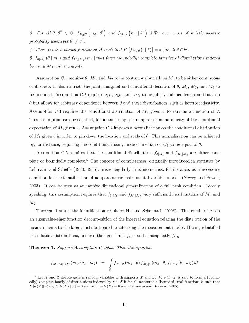
Theorem 1. Suppose Assumption C holds. Then the equation

fM1,M3|M2(m1,m3 | m2) =

ˆ

Θ

fM1|θ (m1 | θ) fM3|θ (m3 | θ) fθ|M2(θ | m2) dθ

5 Let X and Z denote generic random variables with supports X and Z. fX|Z (x | z) is said to form a (bound-edly) complete family of distributions indexed by z ∈ Z if for all measurable (bounded) real functions h such thatE [h (X)] <∞, E [h (X) | Z] = 0 a.s. implies h (X) = 0 a.s. (Lehmann and Romano, 2005).

11

for all m1 ∈M1, m2 ∈M2 and m3 ∈M3 admits unique solutions for fM1|θ, fM3|θ, and fθ|M2.

Let us now turn to the identification of the latent outcome model. This can be achieved by

relating the variation in E [Y |M,D] to the variation in fθ|M,D to the left (D = 0) and to the right

(D = 1) of the cutoff. This is analogous to the identification of nonparametric instrumental variable

models (Newey and Powell, 2003). Assumption D lists the conditions under which E [Y (0) | θ] and

E [Y (1) | θ] are nonparametrically identified for all θ ∈ Θ.

Assumption D.

1. (Y (0) , Y (1)) ⊥⊥M | θ.

2. 0 < P [D = 1 | θ] < 1 a.s.

3. fθ|M,D

(θ | m0, 0

)and fθ|M,D

(θ | m1, 1

)form (boundedly) complete families of distributions

indexed by m0 ∈M0 and m1 ∈M1.

Assumption D.1 requires that Y (0) and Y (1) are related to M only through θ. This can be

thought of as an exclusion restriction. Assumption D.2 requires that the subset of M entering R

are sufficiently noisy measures of θ so that an individual can always end up on either side of the

cutoff. This can be thought of as a common support condition. Assumption D.3 imposes again

a (bounded) completeness condition. This can be thought of as an infinite-dimensional first stage

condition.

Theorem 2 states the identification result. The conditional independence assumption allows

one to write down the integral equations given in the theorem. Under the (bounded) completeness

assumption, E [Y (0) | θ] and E [Y (1) | θ] are unique solutions to these integral equations. Finally,

the common support assumption ensures that both E [Y (0) | θ] and E [Y (1) | θ] are determined

for all θ ∈ Θ.

Theorem 2. Suppose Assumption D holds. Then the equations

E[Y |M = m0, D = 0

]= E

{E [Y (0) | θ] |M = m0, D = 0

}E[Y |M = m1, D = 1

]= E

{E [Y (1) | θ] |M = m1, D = 1

}for all m0 ∈M0 and m1 ∈ M1 admit unique solutions for (bounded) E [Y (0) | θ] and E [Y (1) | θ]

for all θ ∈ Θ.

All of the results discussed in this section can be easily extended to a setting with multidimen-

sional θ. This only requires that one reinterprets θ, M1, and M2 as vectors of the same dimension.

12

M3 can instead still be one-dimensional. Therefore, the data requirements become stricter because

of the additional measures needed for identification, but otherwise all of the results go through.

3 Extension to a Fuzzy RD Design

Section 2 focused on a sharp RD desing where treatment received is fully determined by the running

variable. In this section I discuss an extension to a fuzzy RD design in which treatment received is

only partly determined by the running variable. The fuzziness of the RD design has no implications

on the identification of the measurement model. It only causes modifications to the identification

of the latent outcome model.

In a fuzzy RD design treatment assignment Z ∈ {0, 1} is a deterministic function of the running

variable R and the cutoff c:

Z = 1 (R ≥ c)

However, there is imperfect compliance with the treatment assignment: some of the individuals

assigned to treatment (Z = 1) end up not receiving the treatment (D = 0) whereas some of the

individuals not assigned to treatment (Z = 0) end up receiving the treatment (D = 1). Because of

this, the probability of receiving the treatment jumps at the cutoff but by less than 1:

limδ↓0

P [D = 1 | R = r + δ] > limδ↓0

P [D = 1 | R = r − δ] .

In addition to the potential outcomes Y (0) and Y (1) , each individual is associated with two

potential treatment status: D (0) is the treatment status of an individual if she is not assigned to

the treatment (Z = 0), and D (1) is the treatment status of an individual if she is assigned to the

treatment (Z = 1). The observed outcome and treatment status are

Y = (1−D)× Y (0) +D × Y (1)

D = (1− Z)×D (0) + Z ×D (1) .

Assumption E lists conditions under which the fuzzy RD design allows one to nonparametrically

13

identify the Local Average Treatment Effect (LATE) for the compliers at the cutoff,

E [Y (1)− Y (0) | D (1) > D (0) , R = c] .

The compliers are individuals who are induced to receive the treatment by being assigned the

treatment. Under these assumptions, the LATE is given by the ratio of the discontinuities in

E [Y | R] and E [D | R] at the cutoff, as shown in Lemma 3 (Hahn, Todd, and van der Klaauw,

2001).

Assumption E.

1. fR (r) > 0 in a neighborhood around c.

2. P [D (0) = d0, D (1) = d1 | R = r] are continuous in r at c for d0, d1 = 0, 1.

3. E [Y (0) | D (0) = d0, D (1) = d1, R = r] and E [Y (1) | D (0) = d0, D (1) = d1, R = r] are contin-

uous in r at c for d0, d1 = 0, 1.

4. P [D (1) ≥ D (0) | R = c] = 1 and P [D (1) > D (0) | R = c] > 0

5. E [Y (0) | D (1) > D (0) , R = c] , E [Y (1) | D (1) > D (0) , R = c] <∞.

Lemma 3. (Hahn, Todd, and van der Klaauw, 2001) Suppose Assumption E holds. Then

E [Y (1)− Y (0) | D (1) > D (0) , R = c] = limδ↓0

E [Y | R = c+ δ]− E [Y | R = c− δ]E [D | R = c+ δ]− E [D | R = c− δ]

.

Assumption F lists conditions under which the LATE for compliers at R = r,

E [Y (1)− Y (0) | D (1) > D (0) , R = r] ,

is identified in the latent factor framework. Assumption F.1 requires that the potential outcomes

Y (0) and Y (1) and the potential treatment status D (0) and D (1) are jointly independent of R

conditional on the latent factor θ. Assumption F.2 requires that being assigned the treatment can

only make an individual more likely to receive the treatment for all θ ∈ Θ. Assumption F.3 imposes

this relationship to be strict at least for some individual for all θ ∈ Θ.

Assumption F.

1. (Y (0) , Y (1) , D (0) , D (1)) ⊥⊥ R | θ.

2. P [D (1) ≥ D (0) | θ] = 1 a.s.

3. P [D (1) > D (0) | θ] > 0 a.s.

14

The identification result is stated in Lemma 4. Under Assumption F, the LATE for compliers

at R = r is given by the ratio of the reduced from effect of treatment assignment on the outcome

and the first stage effect of treatment assignment on treatment received at R = r.

Lemma 4. Suppose Assumption F holds. Then

E [Y (1)− Y (0) | D (1) > D (0) , R = r] =E {E [Y (D (1))− Y (D (0)) | θ] | R = r}

E {E [D (1)−D (0) | θ] | R = r}

for all r ∈ R.

Assumption G lists the conditions under which the latent reduced form effect of treatment as-

signment on the outcome, E [Y (D (1))− Y (D (0)) | θ], and the latent first stage effect of treatment

assignment on the probability of receiving the treatment, E [D (1)−D (0) | θ], are nonparametri-

cally identified from the observed conditional expectation functions E [Y |M,Z] and E [D |M,Z].

Assumption G.1 that the noise in M is unrelated to (Y (0) , Y (1) , D (0) , D (1)). Assumption G.2

repeats the common support assumption from Assumption D whereas Assumption G.3 is analogous

to the (bounded) completeness condition in Assumption D.

Assumption G.

1. (Y (0) , Y (1) , D (0) , D (1)) ⊥⊥M | θ.

2. 0 < P [D = 1 | θ] < 1 a.s.

3. fθ|M,Z

(θ | m0, 0

)and fθ|M,Z

(θ | m1, 1

)form (boundedly) complete families of distributions in-

dexed by m0 ∈M0 and m1 ∈M1.

Theorem 3 states the identification result. Together with Lemma 4 this result can be used to

nonparametrically identify the LATE for compliers at any point in the running variable distribution.

The proof of Theorem 3 is analogous to the proof of Theorem 2.

Theorem 3. Suppose Assumption G holds. Then the equations

E[Y |M = m0, D = 0

]= E

{E [Y (D (0)) | θ] |M = m0, D = 0

}E[Y |M = m1, D = 1

]= E

{E [Y (D (1)) | θ] |M = m1, D = 1

}E[D |M = m0, D = 0

]= E

{E [D (0) | θ] |M = m0, D = 0

}E[D |M = m1, D = 1

]= E

{E [D (1) | θ] |M = m1, D = 1

}

15

for all m0 ∈M0 and m1 ∈M1 admit unique solutions for (bounded) E [Y (D (0)) | θ], E [Y (D (1)) | θ],

E [D (0) | θ], and E [D (1) | θ] for all θ ∈ Θ.

4 Boston Exam Schools

4.1 Setting

The BPS system includes three selective high schools, known as exam schools, that span grades 7-12:

Boston Latin School, Boston Latin Academy, and John D. O’Bryant High School of Mathematics

and Science. These schools are seen as the flagship of the BPS system, and they are regularly

among the best high schools in Boston as measured by, for instance, test scores and graduation

rates. Because of their selective admissions process, the exam schools enroll a higher-achieving

student body than traditional BPS schools. In addition, the teaching staff at these schools is more

experienced and qualified, and they offer a rich array of college prepatory classes and extracurricular

activities.

The exam schools admit new students for grades 7 and 9 (O’Bryant also admits some students

for grade 10). Only Boston residents are allowed to apply. Each applicant submits a preference

ordering of the exam schools she is applying to. Admissions decisions are based on the applicant’s

GPA in English and Math from the previous school year and the fall term of the ongoing school

year as well as the applicant’s scores on the ISEE administered during the fall term of the ongoing

school year. The ISEE is an entrance exam used by several selective schools in the United States.

It consists of five sections: Reading Comprehension, Verbal Reasoning, Mathematics Achievement,

Quantitative Reasoning, and a 30-minute essay. Exam school admissions only use the first four

sections of the ISEE.

Each applicant receives an offer from at most one exam school. There is no waitlist practice.

The offers are assigned using the student-proposing Deferred Acceptance (DA) algorithm (Gale and

Shapley, 1962). The algorithm takes as inputs each exam school’s predetermined capacity, each

applicant’s preferences over the exam schools, and the exam schools’ rankings of the applicants

based on a weighted average of their standardized GPA and ISEE scores. These rankings differ

slightly across the exam schools.

The DA algorithm produces exam school-specific admissions cutoffs that are given by the lowest

rank among applicants admitted to a given exam school. Since the applicants receive an offer from

at most one exam school, there is no direct link between an applicant’s rank and offer status.

16

However, as in Abdulkadiroglu, Angrist, and Pathak (2014), it is possible to construct for each

exam school a sharp sample that consists of applicants who receive an offer if and only if their

rank is above the admissions cutoff. Appendix B describes in detail the DA algorithm and the

construction of the sharp samples.

4.2 Data

The data for this paper comes from the following three files provided by the BPS: (1) an exam

school application file, (2) a BPS registration and demographic file, and (3) an Massachusetts

Comprehensive Assessment System (MCAS) file. In addition, I use the students’ home addresses

to merge the BPS data with Census tract-level information from the American Community Survey

(ACS) 5-year summary file for 2006-2011.

The exam school application file consists of the records for all exam school applications in

1995-2009. It provides information on each applicant’s application year and grade, application

preferences, GPA in English and Math, ISEE scores, exam school-specific ranks, and admissions

decision. This allows me to reproduce the exam school-specific admissions cutoffs. I transform the

exam school-specific ranks into percentiles, ranging from 0 to 100, within application year and grade

and center them to be 0 at the admissions cutoff. These exam school-specific running variables

give an applicant’s distance from the admissions cutoff in percentile units. I standardize the ISEE

scores and GPA to have a mean of 0 and a standard deviation of 1 in the applicant population

within each year and grade.

The BPS registration and demographic file consists of the records for all BPS students in 1996-

2012. It provides information on each student’s home address, school, grade, gender, race, limited

English proficiency (LEP) status, bilingual status, special education (SPED) status, and free or

reduced price lunch (FRLP) status.

The MCAS file consists of the records for all MCAS tests taken by BPS students in 1997-2008.

It provides information on 4th, 7th, and 10th grade MCAS scores in English, and 4th, 8th, and

10th grade MCAS scores in Math (in the case of retakes I only consider the first time a student

took the test). I construct middle school and high school MCAS composite scores that are given

by the average of the MCAS scores in 7th grade English and 8th grade Math and the average of

the MCAS scores in 10th grade English and 10th grade Math. I standardize the 4th grade MCAS

scores in English and Math as well as the middle school and high school MCAS composite scores

to have a mean of 0 and standard deviation of 1 in the BPS population within each year and grade.

17

I use the ACS 5-year summary file for 2006-2011 to obtain information on the median fam-

ily income, percent of households occupied by the owner, percent of families headed by a single

parent, percent of households where a language other than English is spoken, distribution of edu-

cational attainment, and number of school-aged children in each Census tract in Boston. I use this

information to divide the Census tracts into socioeconomic tiers as described in Section 6.1.

I restrict the sample to 7th grade applicants in 2000-2004. Most students enter the exam

schools in 7th grade, and their exposure to the exam school treatment is the longest. This is

also the applicant group for which the covariate-based RD extrapolation approach by Angrist

and Rokkanen (forthcoming) fails. The restriction to 2000-2004 allows me to observe both 4th

grade MCAS scores and middle/high school MCAS composite scores for the applicants. I exclude

applicants from outside BPS as they are more likely to remain outside BPS and thus not have

follow-up information in the data.

Table 1 reports descriptive statistics. Column (1) includes all BPS students enrolled in 6th grade

in 2000-2004. Column (2) includes the subset of students who apply to exam schools. Columns

(3)-(6) divide the applicants based on their exam school assignment. Exam school applicants are a

highly selected group of students, with higher 4th grade MCAS scores and lower shares of blacks

and Hispanics, LEP, and SPED. Similarly, there is considerable selection even within exam school

applicants by their exam school assignment, with applicants admitted to a more selective exam

school having higher 4th grade MCAS scores and lower shares of blacks and Hispanics, LEP, and

FRPL.

4.3 Identification and Estimation

Let Z ∈ {0, 1, 2, 3} denote the exam school assignment of an applicant where 0 stands for no offer, 1

for O’Bryant, 2 for Latin Academy and 3 for Latin School. Let S ∈ {0, 1, 2, 3} denote the enrollment

decision of an applicant in the fall following exam school application where 0 stands for traditional

BPS, 1 for O’Bryant, 2 for Latin Academy, and 3 for Latin School. Let R1, R2, and R3 denote the

running variables for O’Bryant, Latin Academy, and Latin School.

The exam school assignment of an applicant is a deterministic function of her running variables

and application preferences, denoted by P :

Z = gZ (R1, R2, R3, P )

18

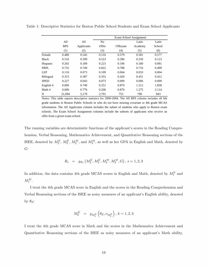
Table 1: Descriptive Statistics for Boston Public School Students and Exam School Applicantsdescriptives

All All No Latin Latin

BPS Applicants Offer O'Bryant Academy School

(1) (2) (3) (4) (5) (6)

Female 0.489 0.545 0.516 0.579 0.581 0.577

Black 0.516 0.399 0.523 0.396 0.259 0.123

Hispanic 0.265 0.189 0.223 0.196 0.180 0.081

FRPL 0.755 0.749 0.822 0.788 0.716 0.499

LEP 0.116 0.073 0.109 0.064 0.033 0.004

Bilingual 0.315 0.387 0.353 0.420 0.451 0.412

SPED 0.227 0.043 0.073 0.009 0.006 0.009

English 4 0.000 0.749 0.251 0.870 1.212 1.858

Math 4 0.000 0.776 0.206 0.870 1.275 2.114

N 21,094 5,179 2,791 755 790 843

Updated: 2013-11-08

Exam School Assignment

Notes: This table reports descriptive statistics for 2000-2004. The All BPS column includes all 6th

grade students in Boston Public Schools in who do not have missing covariate or 4th grade MCAS

information. The All Applicants column includes the subset of students who apply to Boston exam

schools. The Exam School Assignment columns include the subsets of applicants who receive an

offer from a given exam school.

The running variables are deterministic functions of the applicant’s scores in the Reading Compre-

hension, Verbal Reasoning, Mathematics Achievement, and Quantitative Reasoning sections of the

ISEE, denoted by ME2 , ME

3 , MM2 , and MM

3 , as well as her GPA in English and Math, denoted by

G:

Rs = gRs

(ME

2 ,ME3 ,M

M2 ,MM

3 , G), s = 1, 2, 3

In addition, the data contains 4th grade MCAS scores in English and Math, denoted by ME1 and

MM1 .

I treat the 4th grade MCAS score in English and the scores in the Reading Comprehension and

Verbal Reasoning sections of the ISEE as noisy measures of an applicant’s English ability, denoted

by θE :

MEk = gME

k

(θE , νME

k

), k = 1, 2, 3

I treat the 4th grade MCAS score in Math and the scores in the Mathematics Achievement and

Quantitative Reasoning sections of the ISEE as noisy measures of an applicant’s Math ability,

19

Table 2: Correlations between the ISEE Scores and 4th Grade MCAS Scoresmeasurement_correlations

Reading Verbal Math Quantitative English 4 Math 4

(1) (2) (3) (4) (5) (6)

Reading 1 0.735 0.631 0.621 0.670 0.581

Verbal 0.735 1 0.619 0.617 0.655 0.587

Math 0.631 0.619 1 0.845 0.598 0.740

Quantitative 0.621 0.617 0.845 1 0.570 0.718

English 4 0.670 0.655 0.598 0.570 1 0.713

Math 4 0.581 0.587 0.740 0.718 0.713 1.000

Updated: 2013-11-08

Panel B: MCAS

Panel A: ISEE

ISEE MCAS

Notes: This table reports correlations between the ISEE scores and 4th grade MCAS scores. The

sample size is 5,179.

denoted by θM :

MMk = gMM

k

(θM , νMM

k

), k = 1, 2, 3

This generates a two-dimensional latent factor model with θ = (θE , θM ) and Mk =(MEk ,M

Mk

),

k = 1, 2, 3, using the notation of Section 2.

Table 2 reports the correlations between the ISEE scores and 4th grade MCAS scores. The

conrrelations between the test scores are strong but far from perfect. Consistent with the latent

factor structure specified above, test scores measuring English ability are more highly correlated

with each other than with test scores measuring Math ability, and vice versa. There is also a time-

pattern among test scores measuring a given ability: the ISEE scores measuring the same ability

are more highly correlated with each other than with the 4th grade MCAS score measuring the

same ability.

Let Y (s), s = 0, 1, 2, 3, denote potential achievement under different enrollment decisions,

and let S (z), z = 0, 1, 2, 3, denote potential enrollment decisions under different exam school

assignments. I assume that the potential outcomes and enrollment decisions are jointly independent

of the test scores conditional on English and Math abilities and a set of covariates, denoted by X:

({Y (s)}3s=0 , {S (z)}3z=0

)⊥⊥M | θ,X

The covariates included in X are GPA, application preferences, application year, race, gender,

20

SES tier, and indicators for FRPL, LEP, SPED, and being bilingual. I also assume that there is

sufficient noise in the ISEE scores so that conditional on the covariates it is possible to observe an

applicant with a given level of English and Math ability under any exam school assignment:

0 < P [Z = z | θ,X] < 1 a.s., z = 0, 1, 2, 3

These two assumptions are enough to identify causal effects of exam school assignments on

enrollment and achievement. I make two additional assumptions to identify causal effects of en-

rollment at a given exam school as opposed to traditional BPS for the compliers who enroll at the

exam school if they receive an offer and at traditional BPS if they receive no offer. First, I assume

that receiving an offer from exam school s as opposed to no offer induces at least some applicants

to enroll at exam school s instead of traditional BPS. Second, I assume that this is the only way in

which receiving an offer from exam school s as opposed to no offer affects the enrollment decision

of an applicant. Formally, these first stage and monotonicity assumptions are given by

P [S (s) = s, S (0) = 0 | θ,X] > 0, s = 1, 2, 3

P[S (s) = s

′, S (0) = s

′′ | θ,X]

= 0, s′ 6= s, s

′′ 6= 0, s′ 6= s

′′.

The four assumptions made here generalize the fuzzy RD of Section 3 to a setting with multiple

treatments.

I approximate the conditional joint distribution of English and Math ability by a bivariate

normal distribution: θE

θM

| X ∼ N

µ′θEX

µ′θMX

, σ2

θEσθEθM

σθEθM σ2θM

.

To ensure a valid variance-covariance matrix I use the parametrization

σ2θE

σθEθM

σθEθM σ2θM

=

ω11 0

ω21 ω22

ω11 ω21

0 ω22

.

21

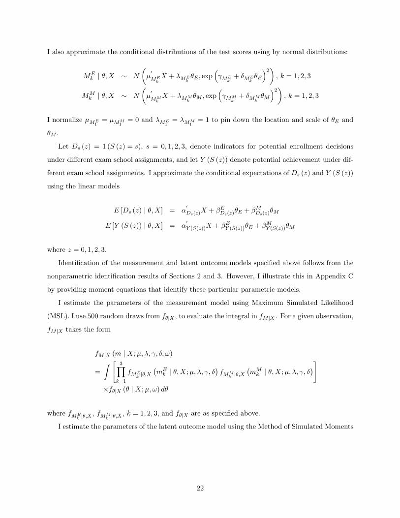
I also approximate the conditional distributions of the test scores using by normal distributions:

MEk | θ,X ∼ N

(µ′

MEkX + λME

kθE , exp

(γME

k+ δME

kθE

)2), k = 1, 2, 3

MMk | θ,X ∼ N

(µ′

MMkX + λMM

kθM , exp

(γMM

k+ δMM

kθM

)2), k = 1, 2, 3

I normalize µME1

= µMM1

= 0 and λME1

= λMM1

= 1 to pin down the location and scale of θE and

θM .

Let Ds (z) = 1 (S (z) = s), s = 0, 1, 2, 3, denote indicators for potential enrollment decisions

under different exam school assignments, and let Y (S (z)) denote potential achievement under dif-

ferent exam school assignments. I approximate the conditional expectations of Ds (z) and Y (S (z))

using the linear models

E [Ds (z) | θ,X] = α′

Ds(z)X + βEDs(z)θE + βMDs(z)θM

E [Y (S (z)) | θ,X] = α′

Y (S(z))X + βEY (S(z))θE + βMY (S(z))θM

where z = 0, 1, 2, 3.

Identification of the measurement and latent outcome models specified above follows from the

nonparametric identification results of Sections 2 and 3. However, I illustrate this in Appendix C

by providing moment equations that identify these particular parametric models.

I estimate the parameters of the measurement model using Maximum Simulated Likelihood

(MSL). I use 500 random draws from fθ|X , to evaluate the integral in fM |X . For a given observation,

fM |X takes the form

fM |X (m | X;µ, λ, γ, δ, ω)

=

ˆ [ 3∏k=1

fMEk |θ,X

(mEk | θ,X;µ, λ, γ, δ

)fMM

k |θ,X(mMk | θ,X;µ, λ, γ, δ

)]×fθ|X (θ | X;µ, ω) dθ

where fMEk |θ,X

, fMMk |θ,X

, k = 1, 2, 3, and fθ|X are as specified above.

I estimate the parameters of the latent outcome model using the Method of Simulated Moments

22

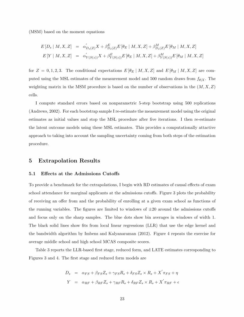
(MSM) based on the moment equations

E [Ds |M,X,Z] = α′

Ds(Z)X + βEDs(Z)E [θE |M,X,Z] + βMDs(Z)E [θM |M,X,Z]

E [Y |M,X,Z] = α′

Y (S(z))X + βEY (S(z))E [θE |M,X,Z] + βMY (S(z))E [θM |M,X,Z]

for Z = 0, 1, 2, 3. The conditional expectations E [θE |M,X,Z] and E [θM |M,X,Z] are com-

puted using the MSL estimates of the measurement model and 500 random draws from fθ|X . The

weighting matrix in the MSM procedure is based on the number of observations in the (M,X,Z)

cells.

I compute standard errors based on nonparametric 5-step bootstrap using 500 replications

(Andrews, 2002). For each bootstrap sample I re-estimate the measurement model using the original

estimates as initial values and stop the MSL procedure after five iterations. I then re-estimate

the latent outcome models using these MSL estimates. This provides a computationally attactive

approach to taking into account the sampling uncertainty coming from both steps of the estimation

procedure.

5 Extrapolation Results

5.1 Effects at the Admissions Cutoffs

To provide a benchmark for the extrapolations, I begin with RD estimates of causal effects of exam

school attendance for marginal applicants at the admissions cutoffs. Figure 3 plots the probability

of receiving an offer from and the probability of enrolling at a given exam school as functions of

the running variables. The figures are limited to windows of ±20 around the admissions cutoffs

and focus only on the sharp samples. The blue dots show bin averages in windows of width 1.

The black solid lines show fits from local linear regressions (LLR) that use the edge kernel and

the bandwidth algorithm by Imbens and Kalyanaraman (2012). Figure 4 repeats the exercise for

average middle school and high school MCAS composite scores.

Table 3 reports the LLR-based first stage, reduced form, and LATE estimates corresponding to

Figures 3 and 4. The first stage and reduced form models are

Ds = αFS + βFSZs + γFSRs + δFSZs ×Rs +X′πFS + η

Y = αRF + βRFZs + γRFRs + δRFZs ×Rs +X′πRF + ε

23

0.2

.4.6

.81

Offe

r P

roba

bilit

y

−20 −10 0 10 20Running Variable

O’Bryant

0.2

.4.6

.81

Offe

r P

roba

bilit

y


Latin Academy

0.2

.4.6

.81

Offe

r P

roba

bilit

y


Latin School

(a) Exam School Offer

0.2

.4.6

.81

Enr

ollm

ent P

roba

bilit

y


O’Bryant

0.2

.4.6

.81

Enr

ollm

ent P

roba

bilit

y


Latin Academy

0.2

.4.6

.81

Enr

ollm

ent P

roba

bilit

y


Latin School

(b) Exam School Enrollment

Figure 3: Relationship between Exam School Offer and Enrollment and the Running Variables

24

−.5

0.5

11.

52

Mea

n S

core


O’Bryant

−.5

0.5

11.

52

Mea

n S

core


Latin Academy

−.5

0.5

11.

52

Mea

n S

core


Latin School

(a) Middle School MCAS Composite Score

−.5

0.5

11.

52

Mea

n S

core


O’Bryant

−.5

0.5

11.

52

Mea

n S

core


Latin Academy

−.5

0.5

11.

52

Mea

n S

core


Latin School

(b) High School MCAS Composite Score

Figure 4: Relationship between Middle School and High School MCAS Composite Scores and theRunning Variables

25

where Ds is an indicator for enrollment at exam school s in the following school year, Y is the

outcome of interest, Zs is an indicator for being at or above the admissions cutoff for exam school

s, Rs is running variable for exam school s, and X is a vector containing indicators for application

years and application preferences. The first stage and reduced form effects are given by βFS and

βRF , and the LATE for compliers at the admissions cutoff is given by βRFβFS

. Columns 1-3 report

estimates for all applicants in the sharp samples. Columns 4-6 and columns 7-9 report estimates

for applicants whose average 4th grade MCAS scores fall below and above the within-year median.

Figure 3a confirms the deterministic nature of exam school offers in the sharp samples: the

probability of receiving an offer from a given exam school jump from 0 to 1 at the admissions

cutoff. However, as can be seen from Figure 3b and the first stage estimates in Table 3, not all

applicants receiving an offer from a given exam school choose to enroll there. The enrollment first

stages are nevertheless large in magnitude, ranging from around 0.7-0.8 for O’Bryant to around

0.9-1.0 for Latin Academy and Latin School.

According to Figure 4a and the reduced form estimates in Panel A of Table 3, access to Latin

Academy reduces the average middle school MCAS composite score of marginal applicants by

0.181σ. The corresponding estimates for O’Bryant and Latin School are also negative but not

statistically significant. These negative effects are concentrated among applicants with high 4th

grade MCAS scores. The estimates for applicants with low 4th grade MCAS scores are instead

positive (although not statistically signicant), with the exception of Latin School. The LATE

estimates are similar to the reduced from estimates because of the high enrollment first stages.

According to Figure 4b and the reduced form estimates in Panel B of Table 3, there is no

statistically significant evidence of effects of access to the exam schools on the average high school

MCAS composite score of marginal applicants. There is, however, some evidence of heterogeneity in

these effects: access to O’Bryant is estimated to increase the average high school MCAS composite

score of marginal applicants with low 4th grade MCAS scores by 0.204σ. The LATE estimates are

again similar to the reduced from estimates because of the high enrollment first stages.

It is important to note the incremental nature of the RD estimates reported here. Applicants

just below the O’Bryant admissions cutoff do not receive an offer from any exam school. Therefore,

the counterfactual for these applicants is traditional BPS. On the other hand, the vast majority

of applicants just below the Latin Academy admissions cutoff receive an offer from O’Bryant, and

the vast majority of applicants just below the Latin School admissions cutoff receive an offer from

Latin Academy. This means that for most of the applicants at the Latin Academy admissions

26

Table 3: RD Estimates of the First Stage, Reduced Form and Local Average Treatment Effects atthe Admissions Cutoffs

rd_estimates

Latin Latin Latin Latin Latin Latin

O'Bryant Academy School O'Bryant Academy School O'Bryant Academy School

(1) (2) (3) (4) (5) (6) (7) (8) (9)

First 0.775*** 0.949*** 0.962*** 0.734*** 0.917*** 1.000*** 0.780*** 0.956*** 0.961***

Stage (0.031) (0.017) (0.017) (0.072) (0.056) (0.000) (0.033) (0.017) (0.017)

Reduced -0.084 -0.181*** -0.104 0.059 0.130 -0.095 -0.122* -0.200*** -0.084

Form (0.060) (0.057) (0.079) (0.127) (0.199) (0.214) (0.065) (0.056) (0.082)

LATE -0.108 -0.191*** -0.108 0.080 0.142 -0.095 -0.157* -0.209*** -0.088

(0.078) (0.060) (0.082) (0.173) (0.215) (0.214) (0.083) (0.059) (0.085)

N 1,934 2,328 1,008 420 246 681 1,348 1,802 921

First 0.781*** 0.955*** 0.964*** 0.742*** 0.944*** 1.000*** 0.797*** 0.942*** 0.964***

Stage (0.034) (0.018) (0.018) (0.074) (0.055) (0.000) (0.033) (0.022) (0.017)

Reduced 0.047 -0.021 -0.086 0.204** -0.029 -0.272 0.017 -0.029 -0.093*

Form (0.055) (0.044) (0.052) (0.099) (0.141) (0.186) (0.054) (0.052) (0.053)

LATE 0.060 -0.022 -0.089 0.275** -0.031 -0.272 0.021 -0.030 -0.097*

(0.070) (0.046) (0.054) (0.136) (0.150) (0.186) (0.068) (0.055) (0.055)

N 1,475 1,999 907 531 567 436 1,129 974 909

Updated: 2013-11-08

All Applicants

Notes: This table reports RD estimates of the effect of an exam school offer on exam school enrollment (First Stage), the

effect of an exam school offer on MCAS scores (Reduced Form), and the effects of exam school enrollment on MCAS

scores (LATE). The estimates are shown for all applicants as well as separately for applicants whose average 4th grade

MCAS scores fall below and above the within-year median. Heteroskedasticity-robust standard errors shown in

parentheses.

Panel A: Middle School MCAS

Panel B: High School MCAS

* significant at 10%; ** significant at 5%; *** significant at 1%

Low 4th Grade MCAS High 4th Grade MCAS

27

cutoff the relevant counterfactual is O’Bryant whereas at the Latin School admissions cutoff the

relevant counterfactua is Latin Academy. Therefore, the above estimates should be interpreted as

incremental effects of gaining access or going to a more selective school.

5.2 Estimates of the Latent Factor Model

Before turning to the extrapolation results I briefly discuss the main estimates of the measurement

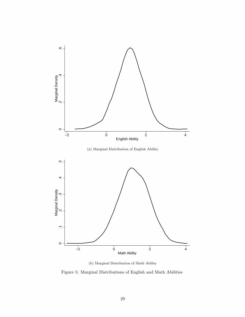
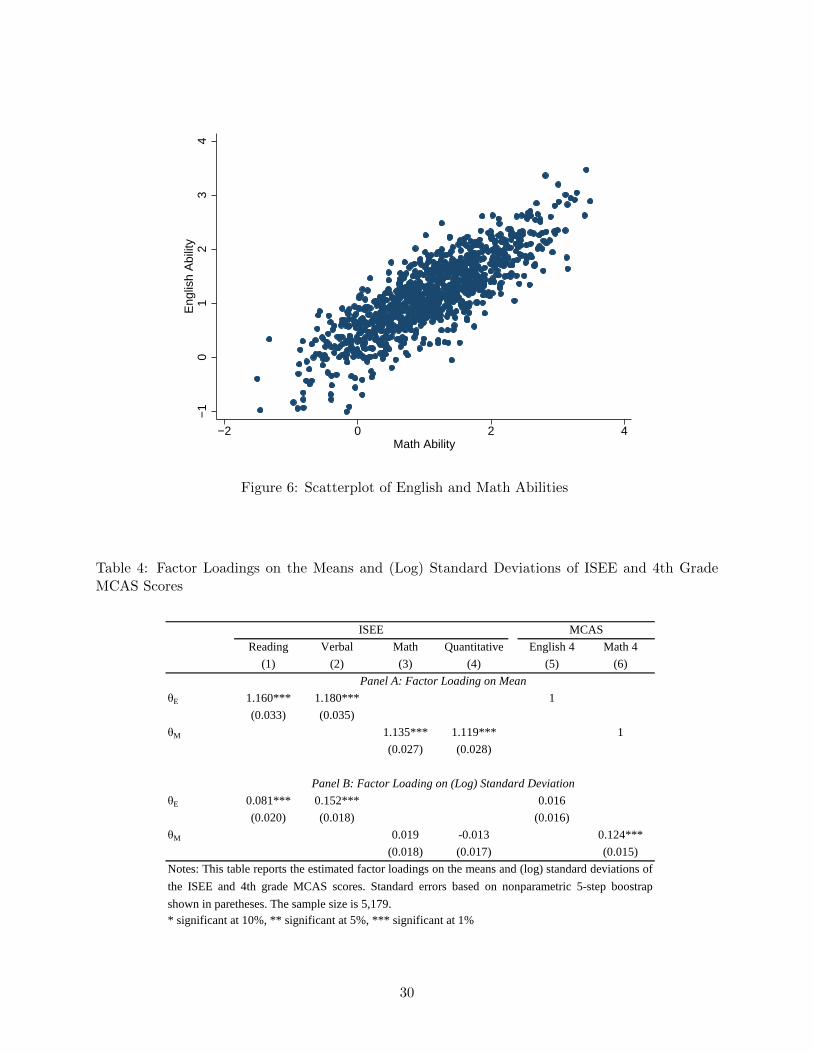
and latent outcome models. Figures 5 and 6 show the marginal distributions and scatterplot of

English and Math ability among exam school applicants based on simulations from the estimated

measurement model. The mean and standard deviation of English ability are 1.165 and 0.687. The

mean and standard deviation of Math ability are 1.121 and 0.831. The correlation between the two

abilities is 0.817.

Table 4 reports the estimated factor loadings on the means and (log) standard deviations of

ISEE and 4th grade MCAS scores. As mentioned above, the scales of the abilities have been

pinned down by normalizing the factor loadings on the means of 4th grade MCAS scores to 1. The

estimated factor loadings on the means of ISEE scores are somewhat above 1. The estimated factor

loadings on the (log) standard deviations of ISEE scores in Reading Comprehension and Verbal

Reasoning and 4th grade MCAS score in Math suggest that the variances of these test scores are

increasing in the relevant ability. The estimated factor loadings on the (log) standard deviations

of ISEE scores in Mathematical Achievement and Quantitative Reasoning and 4th grade MCAS

score in English are small in magnitude and statistically insignificant.

Table 5 reports the estimated factor loadings on enrollment (First Stage) and middle school

and high school MCAS composite scores (Reduced Form) under a given exam school assignment.

For no exam school offer in column 1 the enrollment outcome is enrollment at traditional BPS. For

an offer from a given exam school in columns 2-4 the outcome is enrollment at the exam school in

question. With the exception of Latin School, the estimated factor loadings on enrollment tend to

be negative, suggesting that applicants with higher ability are less likely to attend a given exam

school if they receive an offer (or traditional BPS if they receive no offer). However, most of the

estimates are small in magnitude and statistically insignificant.

The estimated factor loadings on middle school and high school MCAS composite scores are

positive, large in magnitude, and statistically significant. This is not surprising: applicants with

higher English and Math abilities tend to perform, on average, better in middle school and high

school English and Math irrespective of their exam school assignment. A more interesting finding

28

0.2

.4.6

Mar

gina

l Den

sity

−2 0 2 4English Ability

(a) Marginal Distribution of English Ability

0.1

.2.3

.4.5

Mar

gina

l Den

sity

−2 0 2 4Math Ability

(b) Marginal Distribution of Math Ability

Figure 5: Marginal Distributions of English and Math Abilities

29

−1

01

23

4E

nglis

h A

bilit

y

−2 0 2 4Math Ability

Figure 6: Scatterplot of English and Math Abilities

Table 4: Factor Loadings on the Means and (Log) Standard Deviations of ISEE and 4th GradeMCAS Scores

factor_loadings

Reading Verbal Math Quantitative English 4 Math 4

(1) (2) (3) (4) (5) (6)

θE 1.160*** 1.180*** 1

(0.033) (0.035)

θM 1.135*** 1.119*** 1

(0.027) (0.028)

θE 0.081*** 0.152*** 0.016

(0.020) (0.018) (0.016)

θM 0.019 -0.013 0.124***

(0.018) (0.017) (0.015)

Updated: 2014-03-31

Notes: This table reports the estimated factor loadings on the means and (log) standard deviations of

the ISEE and 4th grade MCAS scores. Standard errors based on nonparametric 5-step boostrap

shown in paretheses. The sample size is 5,179.

* significant at 10%, ** significant at 5%, *** significant at 1%

Panel B: Factor Loading on (Log) Standard Deviation

ISEE MCAS

Panel A: Factor Loading on Mean

30

Table 5: Factor Loadings on Enrollment and MCAS Scores Under Given Exam School Assignments

latent_fs_rf

No Latin Latin No Latin Latin

Offer O'Bryant Academy School Offer O'Bryant Academy School

(1) (2) (3) (4) (5) (6) (7) (8)

θE -0.001 -0.073 -0.107** 0.016 -0.001 -0.025 -0.102* 0.003

(0.007) (0.069) (0.050) (0.011) (0.011) (0.076) (0.053) (0.009)

θM -0.008 -0.035 0.011 0.023 -0.012 -0.059 0.012 0.027**

(0.006) (0.059) (0.031) (0.015) (0.008) (0.061) (0.030) (0.012)

θE 0.570*** 0.476*** 0.190** 0.439*** 0.446*** 0.282*** 0.217*** 0.239***

(0.052) (0.087) (0.089) (0.063) (0.062) (0.067) (0.066) (0.046)

θM 0.633*** 0.601*** 0.742*** 0.464*** 0.604*** 0.346*** 0.267*** 0.158***

(0.050) (0.067) (0.067) (0.063) (0.056) (0.070) (0.057) (0.044)

N 2,490 690 728 793 1,777 563 625 793

Updated: 2014-03-31


Panel A: First Stage

Panel B: Reduced Form

Middle School MCAS High School MCAS

Notes: This table reports the estimated factor loadings on enrollment (First Stage) and MCAS scores (Reduced

Form) under a given exam school assignment. First Stage refers to enrollment at a traditional Boston public school

in the No Offer column and enrollment at a given exam school in the other columns. Standard errors based on

nonparametric 5-step boostrap shown in paretheses.

is that the factor loadings are larger in magnitude under no offer than under an offer from any

given exam school. This is especially true for high school MCAS composite scores. This suggest

that applicants with lower English and Math abilities gain more in terms of their achievement from

access to exam schools.

5.3 Effects Away from the Admissions Cutoffs

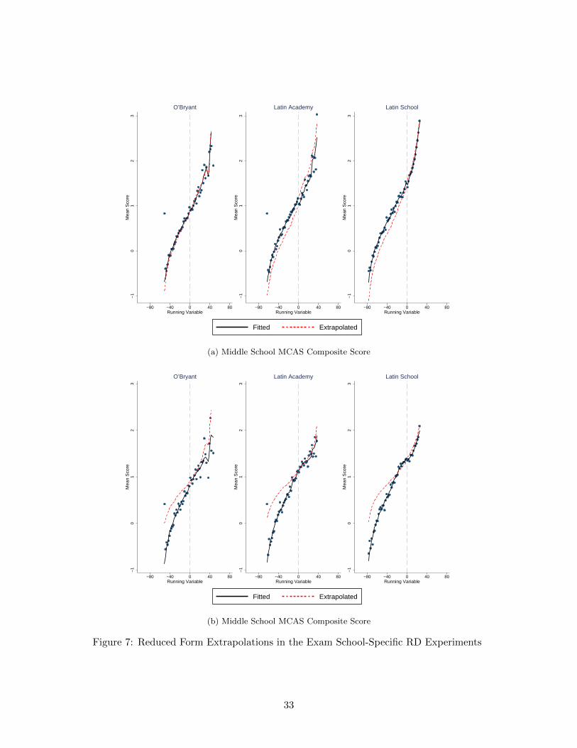
Figure 7 plots the latent factor model-based fits and extrapolations for the sharp samples in the

RD experiments over the full supports of the running variables. The fits and extrapolations are

defined as

E[Y(S(zact

))| Rs = r

], s = 1, 2, 3

E[Y(S(zcf))| Rs = r

], s = 1, 2, 3

where the counterfactual assignment zcf is an offer from exam school s for applicants below the

admissions cutoff for exam school s and an offer from the next most selective exam school for the

31

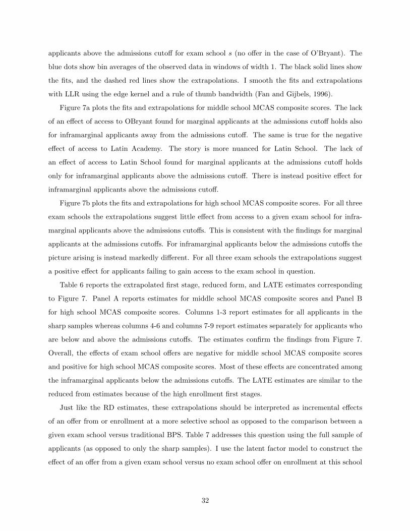
applicants above the admissions cutoff for exam school s (no offer in the case of O’Bryant). The

blue dots show bin averages of the observed data in windows of width 1. The black solid lines show

the fits, and the dashed red lines show the extrapolations. I smooth the fits and extrapolations

with LLR using the edge kernel and a rule of thumb bandwidth (Fan and Gijbels, 1996).

Figure 7a plots the fits and extrapolations for middle school MCAS composite scores. The lack

of an effect of access to OBryant found for marginal applicants at the admissions cutoff holds also

for inframarginal applicants away from the admissions cutoff. The same is true for the negative

effect of access to Latin Academy. The story is more nuanced for Latin School. The lack of

an effect of access to Latin School found for marginal applicants at the admissions cutoff holds

only for inframarginal applicants above the admissions cutoff. There is instead positive effect for

inframarginal applicants above the admissions cutoff.

Figure 7b plots the fits and extrapolations for high school MCAS composite scores. For all three

exam schools the extrapolations suggest little effect from access to a given exam school for infra-

marginal applicants above the admissions cutoffs. This is consistent with the findings for marginal

applicants at the admissions cutoffs. For inframarginal applicants below the admissions cutoffs the

picture arising is instead markedly different. For all three exam schools the extrapolations suggest

a positive effect for applicants failing to gain access to the exam school in question.

Table 6 reports the extrapolated first stage, reduced form, and LATE estimates corresponding

to Figure 7. Panel A reports estimates for middle school MCAS composite scores and Panel B

for high school MCAS composite scores. Columns 1-3 report estimates for all applicants in the

sharp samples whereas columns 4-6 and columns 7-9 report estimates separately for applicants who

are below and above the admissions cutoffs. The estimates confirm the findings from Figure 7.

Overall, the effects of exam school offers are negative for middle school MCAS composite scores

and positive for high school MCAS composite scores. Most of these effects are concentrated among

the inframarginal applicants below the admissions cutoffs. The LATE estimates are similar to the

reduced from estimates because of the high enrollment first stages.

Just like the RD estimates, these extrapolations should be interpreted as incremental effects

of an offer from or enrollment at a more selective school as opposed to the comparison between a

given exam school versus traditional BPS. Table 7 addresses this question using the full sample of

applicants (as opposed to only the sharp samples). I use the latent factor model to construct the

effect of an offer from a given exam school versus no exam school offer on enrollment at this school

32

−1

01

23

Mea

n S

core


O’Bryant

−1

01

23

Mea

n S

core


Latin Academy

−1

01

23

Mea

n S

core


Latin School

Fitted Extrapolated


−1

01

23

Mea

n S

core


O’Bryant

−1

01

23

Mea

n S

core


Latin Academy

−1

01

23

Mea

n S

core


Latin School

Fitted Extrapolated

(b) Middle School MCAS Composite Score

Figure 7: Reduced Form Extrapolations in the Exam School-Specific RD Experiments

33

Table 6: Extrapolated First Stage, Reduced Form, and Local Average Treatment Effects in theExam School-Specific RD Experiments

rd_extrapolation



(1) (2) (3) (4) (5) (6) (7) (8) (9)

First 0.869*** 0.971*** 0.950*** 0.904*** 0.992*** 0.960*** 0.749*** 0.891*** 0.906***

Stage (0.033) (0.013) (0.017) (0.041) (0.015) (0.020) (0.016) (0.018) (0.031)

Reduced -0.047 -0.229** -0.214*** -0.050 -0.234* -0.245** -0.038 -0.211*** -0.080

Form (0.093) (0.100) (0.080) (0.118) (0.123) (0.097) (0.034) (0.061) (0.076)

LATE -0.054 -0.236** -0.226*** -0.055 -0.236* -0.255** -0.051 -0.237*** -0.088

(0.108) (0.103) (0.084) (0.132) (0.124) (0.101) (0.045) (0.069) (0.085)

N 3,029 3,641 4,271 2,339 2,913 3,478 690 728 793

First 0.858*** 0.962*** 0.950*** 0.892*** 0.984*** 0.959*** 0.758*** 0.885*** 0.920***

Stage (0.038) (0.021) (0.018) (0.050) (0.027) (0.021) (0.017) (0.021) (0.029)

Reduced 0.252*** 0.279*** 0.199*** 0.343*** 0.362*** 0.281*** -0.021 -0.005 -0.091*

Form (0.068) (0.075) (0.061) (0.089) (0.092) (0.075) (0.034) (0.046) (0.054)

LATE 0.293*** 0.290*** 0.209*** 0.385*** 0.367*** 0.293*** -0.028 -0.006 -0.099*

(0.081) (0.079) (0.064) (0.102) (0.097) (0.079) (0.045) (0.053) (0.059)

N 2,240 2,760 3,340 1,677 2,135 2,601 563 625 739

Updated: 2014-03-31

Below Admissions Cutoff Above Admissions CutoffAll Applicants



Notes: This table reports latent factor model based-estimates of the effect of an exam school offer on exam school

enrollment (First Stage), the effect of an exam school offer on MCAS scores (Reduced Form), and the effects of exam

school enrollment on MCAS scores (LATE) in the RD experiments. The estimates are shown for all applicants as wells

as separately for applicants whose running variables fall below and above the admissions cutoffs.Standard errors based

on nonparametric 5-step boostrap shown in paretheses.


34

(first stage) and on achievement (reduced form):

E [Ds (s)−Ds (0)] , s = 1, 2, 3

E [Y (S (s))− Y (S (0))] , s = 1, 2, 3

I use these first stage and reduced form effects to construct the LATE of enrollment at a given

exam school versus a traditional BPS for the full population of compliers induced to enroll at the

exam school in question as opposed to traditional BPS:

E [Y (s)− Y (0) | Ds (s) = 1, D0 (0) = 1] =E [Y (S (s))− Y (S (0))]

E [Ds (s)−Ds (0)], s = 1, 2, 3

Panel A reports the estimates for middle school MCAS composite scores and Panel B for high

school MCAS composite scores. Columns 1-3 report estimates for all applicants whereas columns

4-6 and columns 7-9 report estimates separately for low-scoring applicants who do not receive an

exam school offer and for high-scoring applicants who receive an exam school offer.

The estimates for middle school MCAS composite scores show large negative effects from re-

ceiving offers from Latin Academy and Latin School and no effect from receiving an offer from

O’Bryant. There is not much evidence of heterogeneity in these effects by admissions status. The

estimates for high school MCAS composite scores show instead no effect for the full population

of applicants, but there is considerable heterogeneity in these effects by admissions status. For

all three schools the estimates show large negative effects for low-scoring applicants who do not

receive an exam school offer and large positive effects for high-scoring applicants who receive an

exam school offer.

5.4 Placebo Experiments

A concern one might have with the previous results is that they are just an artifact of arbitrary

extrapolations away from the admissions cutoffs. To address this concern, I study the performance

of the latent factor model using a set of placebo experiments. I split the applicants with exam

school assignment z = 0, 1, 2, 3 in half based on the within-year median of the running variable.6

I re-estimate the latent outcome models to the left and right of the resulting placebo cutoffs and

use the these estimates to extrapolate away from the placebo cutoffs. All of the applicants to the

6For applicant receiving no offer I use the average of their exam school-specific running variables.

35

Table 7: Extrapolated First Stage, Reduced Form, and Local Average Treatment Effects for Com-parisons between a Given Exam School and Traditional Boston Public Schools

extrapolation



(1) (2) (3) (4) (5) (6) (7) (8) (9)

First 0.767*** 0.956*** 0.967*** 0.901*** 0.994*** 0.958*** 0.749*** 0.927*** 0.986***

Stage (0.017) (0.009) (0.016) (0.040) (0.016) (0.024) (0.016) (0.010) (0.005)

Reduced -0.059 -0.275*** -0.319*** -0.051 -0.246* -0.279** -0.069 -0.307*** -0.363***

Form (0.048) (0.074) (0.079) (0.117) (0.138) (0.117) (0.074) (0.048) (0.051)

LATE -0.077 -0.288*** -0.330*** -0.057 -0.248* -0.292** -0.092 -0.332*** -0.368***

(0.063) (0.078) (0.082) (0.131) (0.140) (0.122) (0.099) (0.052) (0.052)

N

First 0.754*** 0.948*** 0.968*** 0.887*** 0.987*** 0.955*** 0.758*** 0.925*** 0.987***

Stage (0.020) (0.013) (0.016) (0.049) (0.030) (0.026) (0.017) (0.010) (0.005)

Reduced 0.021 0.049 0.024 0.334*** 0.429*** 0.428*** -0.268*** -0.300*** -0.348***

Form (0.037) (0.058) (0.064) (0.088) (0.105) (0.094) (0.066) (0.048) (0.052)

LATE 0.027 0.052 0.025 0.376*** 0.435*** 0.448*** -0.353*** -0.325*** -0.353***

(0.049) (0.062) (0.066) (0.102) (0.110) (0.098) (0.087) (0.053) (0.053)

N

Updated: 2014-03-31

No Exam School Offer Exam School Offer

2,490 2,211

All Applicants



Notes: This table reports latent factor model based-estimates of the effect of receiving an offer from a given exam school

versus no offer at all on enrollment at this exam school (First Stage), the effect of receiving an offer from a given exam

school versus no offer at all on MCAS scores (Reduced Form), and the effect of enrollment at this exam school versus a

traditional Boston public school on MCAS scores (LATE). The estimates are shown for all applicants as well as separately

for applicants who do not receive an exam school offer and for applicants who receive an exam school offer. Standard

errors based on nonparametric 5-step boostrap shown in paretheses.


1,777 1,927

4,701

3,704

36

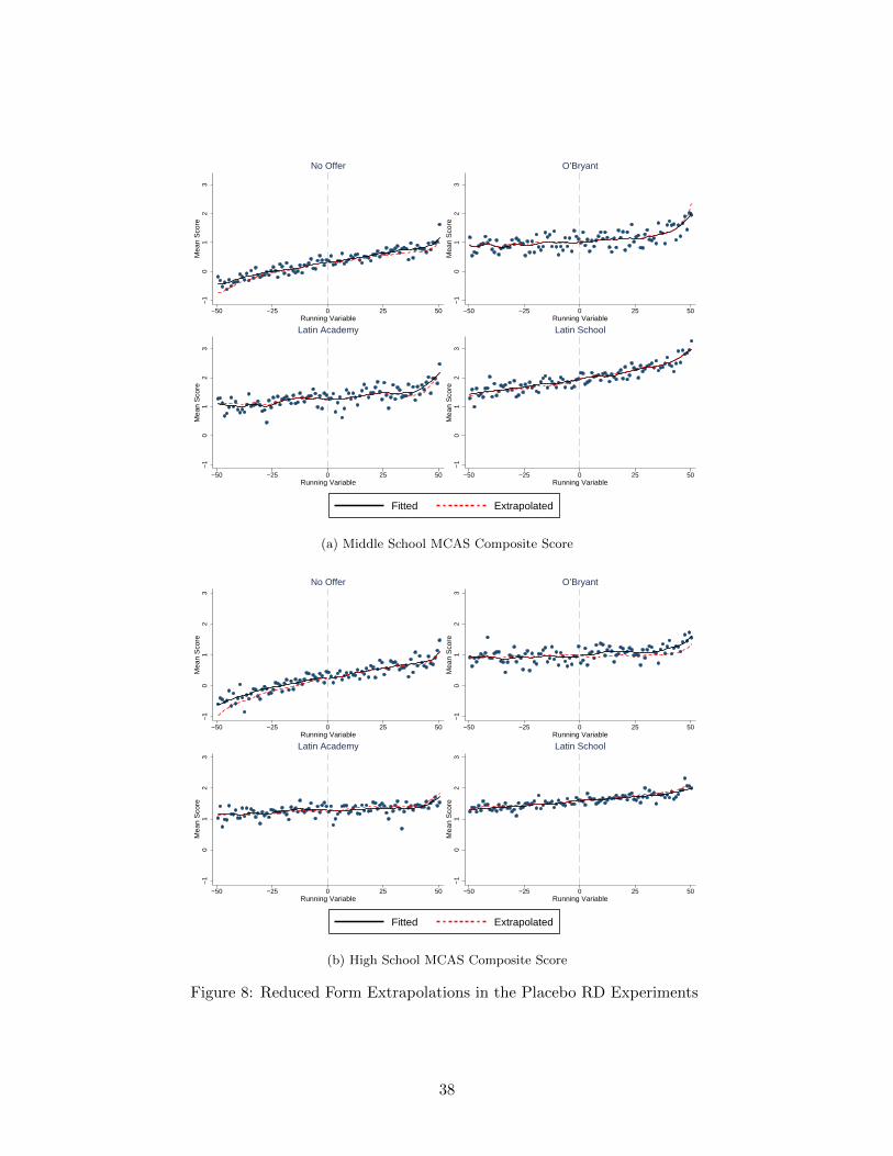
left and right of the placebo cutoffs receive the same exam school assignment. Therefore, these

extrapolations should show no effects if the identifying assumptions are valid and the empirical

specifications provide reasonable approximations to the underlying data generating processes.

Figure 8 plots the fits and extrapolations in the placebo RD experiments.7 The corresponding

placebo estimates are reported in table 8. The fits and extrapolations lie close to each other, and the

corresponding placebo effects are small in magnitude and statistically insignificant. This provides

strong evidence supporting the identifying assumptions and empirical specifications.

6 Counterfactual Simulations

6.1 Description of the Admissions Reforms

Estimates of exam school effects away from the admissions cutoffs are useful for predicting effects of

reforms that change the exam school assignments of inframarginal applicants. A highly contentious

example of this is the introduction of affirmative action in the currently purely achievement-based

exam school admissions. I use the estimated latent factor model to predict how two particular

affirmative action reforms would affect the achievement of exam school applicants.

The first reform considers minority preferences that were in place in Boston exam school ad-

missions in 1975-1998. In this counterfactual admissions process 65% of the exam school seats are

first assigned among all applicants. The remaining 35% of the exam school seats are then assigned

among black and Hispanic applicants.

The second reform considers socioeconomic preferences that have been in place in Chicago exam

school admissions since 2010. In this counterfactual admissions process 30% of the exam school

seats are first assigned among all applicants. The remaining 70% of the exam school seats are then

assigned within four sosioeconomic tiers.8

7I transform the running variables into percentile ranks within each year in the placebo RD experiments andre-centered them to be 0 at the placebo cutoff for expositional purposes.

8The socioeconomic tiers are constructed by computing for each Census tract in Boston a socioeconomic index thattakes into account the following five characteristics: (1) median family income, (2) percent of households occcupiedby the owner, (3) percent of families headed by a single parent, (4) percent of households where a language other thanEnglish is spoken, and (5) an educational attainment score. The educational attainment score is calculated based onthe educational attainment distribution among individuals over the age of 25: educational attainment score = 0.2×(% less thanhigh school diploma)+0.4×(%high school diploma)+0.6×(% some college)+0.8×(% bachelors degree)+1.0 × (% advanced degree). The socioeconomic index for a given Census tract is given by the sum of its percentileranks in each five characteristics among the Census tracts in Boston (for single-parent and non-English speaking

37

−1

01

23

Mea

n S

core


No Offer

−1

01

23

Mea

n S

core


O’Bryant

−1

01

23

Mea

n S

core


Latin Academy

−1

01

23

Mea

n S

core


Latin School

Fitted Extrapolated


−1

01

23

Mea

n S

core


No Offer

−1

01

23

Mea

n S

core


O’Bryant

−1

01

23

Mea

n S

core


Latin Academy

−1

01

23

Mea

n S

core


Latin School

Fitted Extrapolated

(b) High School MCAS Composite Score

Figure 8: Reduced Form Extrapolations in the Placebo RD Experiments

38

Table 8: Extrapolated Reduced Form Effects in the Placebo RD Experimentsplacebo

No Latin Latin

Offer O'Bryant Academy School

(1) (2) (3) (4)

Middle 0.002 -0.000 0.042 -0.023

School (0.053) (0.089) (0.081) (0.072)

MCAS 2,490 690 728 793

High -0.057 0.080 -0.041 -0.008

School (0.064) (0.068) (0.062) (0.045)

MCAS 1,777 563 625 793

Middle -0.081 0.015 0.034 -0.034

School (0.082) (0.075) (0.069) (0.067)

MCAS 1,244 344 362 395

High -0.133 0.027 -0.028 0.027

School (0.099) (0.061) (0.055) (0.049)

MCAS 887 280 311 368

Middle 0.085* -0.015 0.050 -0.013

School (0.048) (0.134) (0.127) (0.112)

MCAS 1,246 346 366 395

High 0.020 0.133 -0.054 -0.044

School (0.056) (0.102) (0.097) (0.068)

MCAS 890 283 314 371

Updated: 2014-03-31

Panel A: All Applicants

Panel B: Below Placebo Cutoff

Panel C: Above Placebo Cutoff

Notes: This table reports latent factor model-based estimates

of the effects of placebo offers on MCAS scores. The

estimates are shown for all applicants and separately for

applicants whose running variables fall below and above the

placebo admissions cutoffs. Standard errors based on


* significant at 10%, ** significant at 5%, *** significant at

1%

39

To study the effects of the two reforms I reassign exam school offers based on the counterfactual

admissions processes, considering only applicants in the estimation sample. I then use the estimated

latent factor model to predict average middle school and high school MCAS composite scores based

on the reassigned exam school offers.9

An important feature of both of the reforms is that they cause substantial changes to the

admissions cutoffs faced by exam school applicants. This means that predictions of the effects of

the reforms based on exam school effects at the admissions cutoffs are likely to be misleading if

there is considerable heterogeneity in the effects based on the running variables. Based on the

results above, this is the case for Boston exam schools.

As with all counterfactuals, there are other dimensions that may also chance as a result. First,

the reforms potentially affect the composition of the pool of exam school applicants as some student

face a decrease and some students an increase in their ex ante expected probability of being admitted

to a given exam school.10 Second, the reforms lead to changes in the composition of applicants

who are admitted to and consequently enroll at the exam schools. These changes may affect the

sorting of teachers across schools (Jackson, 2009) and the way teaching is targeted (Duflo, Dupas,

and Kremer, 2011). Finally, the changes in student composition may affect achievement directly

through peer effects (Epple and Romano, 2011; Sacerdote, 2011).

6.2 Simulation Results

The introduction of minority and socioeconomic preferences have substantial effects on the exam

school assigments. They lower the admissions cutoffs faced by minority applicants and applicants

from lower socioeconomic tiers and increase the admissions cutoffs faced by non-minority applicants

and applicants from higher socioeconomic tiers. Overall, 27− 35% of the applicants are affected by

the reforms. This can be seen from Table 9 that reports the actual and counterfactual exam school

assignments.

Table 10 reports descriptive statistics for the exam school applicants based on their counterfac-

tual assignments. The most notable compositional changes caused by the two reforms can be seen

households 1 minus the percentile rank). Each BPS student is assigned a socioeconomic index based on the Censustract they live in and the students are divided into socioecomic tiers based on the quartiles of the socioeconomicindex distribution in the BPS population within each year.

9This exercise is closely related to the literatute on evaluating the effects of reallocations on the distribution ofoutcomes (Graham, 2011).

10Long (2004) and Andrews, Ranchhod, and Sathy (2010) find the college application behavior of high schoolstudents in California and Texas to be responsive to affirmative action. However, the evidence on this is somewhatmixed (Card and Krueger, 2005; Antonovics and Backes, 2013).

40

Table 9: Actual and Counterfactual Assignments under Minority and Socioeconomic Preferencescfsim12_assignments

No Latin Latin

Counterfactual Offer O'Bryant Academy School

Assignment (1) (2) (3) (4)

No Offer 2418 221 113 39

O'Bryant 280 129 133 213

Latin Academy 88 389 268 45

Latin School 5 16 276 546

No Offer 2579 159 39 14

O'Bryant 203 319 146 87

Latin Academy 9 106 403 272

Latin School 0 171 202 470

Updated: 2013-11-08

Actual Assignment

Panel A: Minority Preferences

Panel B: Socioeconomic Preferences

Notes: This table reports the actual assignments and the

counterfactual assignments under minority and socioeconomic

preferences in the exam school admissions.

among applicants receiving no exam school offer and among applicants receiving an offer from Latin

School. The reforms reduce baseline achievement and increase the share of minority applicants in

the former group while having the opposite effects for the latter group. There are less marked

changes in the composition of applicants receiving offers from O’Bryant and Latin Academy.

Table 11 reports the Average Reassignment Effects (ARE) of the reforms on middle school

and high school MCAS composite scores. The ARE is given by the difference in average potential

achievement among exam school applicants under the counterfactual and actual assignments:

E[Y cf − Y act

]=

3∑z′=0

3∑z′′=0

P[Zcf = z

′, Zact = z

′′]E[Y(S(z′))− Y

(S(z′′))| Zcf = z

′, Zact = z

′′]

where Zact and Zcf are an applicant’s actual and counterfactual assignments. Panel A reports the

ARE estimates for full population of applicants and Panel B for applicants whose assignment is

affected by the reform (Zact 6= Zcf ).

The estimates for middle school MCAS composite scores show no effect of either reform on the

average score among the full population of applicants. However, there is substantial heterogeneity

in these effects. Introduction of minority preferences is estimated to reduce the average score

41

Table 10: Composition of Applicants by Counterfactual Assignments under Minority and Socioe-conomic Preferences

cfsim12_descriptives

No Latin Latin

Offer O'Bryant Academy School

(1) (2) (3) (4)

Female 0.502 0.588 0.629 0.572

Black 0.430 0.440 0.386 0.274

Hispanic 0.182 0.220 0.203 0.172

FRPL 0.810 0.771 0.715 0.556

LEP 0.116 0.030 0.022 0.018

Bilingual 0.386 0.396 0.380 0.391

SPED 0.073 0.009 0.013 0.005

English 4 0.277 0.981 1.215 1.668

Math 4 0.277 0.963 1.289 1.781

Female 0.514 0.572 0.597 0.575

Black 0.499 0.360 0.295 0.203

Hispanic 0.223 0.191 0.143 0.120

FRPL 0.813 0.728 0.673 0.624

LEP 0.107 0.058 0.030 0.017

Bilingual 0.359 0.423 0.391 0.445

SPED 0.073 0.012 0.006 0.006

English 4 0.261 1.067 1.309 1.556

Math 4 0.217 1.146 1.365 1.744

N 2,791 755 790 843

Updated: 2013-11-08

Panel A: Minority Preferences

Panel B: Socioeconomic Preferences

Notes: This table reports descriptive statistics for the exam school

applicants by their counterfactual assignment under minority and

socioeconomic preferences in the exam school admissions.

42

Table 11: Average Reassignment Effects of Introducing Minority or Socioeconomic Preferencescfsim12_effects

All Non- All SES SES SES SES

Applicants Minority Minority Applicants Tier 1 Tier 2 Tier 3 Tier 4

(1) (2) (3) (4) (5) (6) (7) (8)

Middle 0.001 -0.028*** 0.043*** 0.007 -0.032*** -0.005 0.004 0.041***

School (0.005) (0.007) (0.010) (0.005) (0.011) (0.006) (0.007) (0.011)

MCAS 4,701 2,741 1,960 4,701 948 1,113 1,155 1,468

High 0.023*** 0.027*** 0.017* 0.015*** 0.024** 0.011* 0.006 0.018*

School (0.004) (0.007) (0.009) (0.005) (0.011) (0.006) (0.005) (0.010)

MCAS 3,704 2,086 1,618 3,704 737 876 901 1,190

Middle 0.003 -0.084*** 0.113*** 0.024 -0.092*** -0.021 0.021 0.133***

School (0.014) (0.021) (0.026) (0.019) (0.032) (0.027) (0.031) (0.034)

MCAS 1,670 932 738 1,294 328 263 241 426

High 0.062*** 0.074*** 0.046** 0.050*** 0.068** 0.044* 0.026 0.054*

School (0.011) (0.017) (0.020) (0.016) (0.031) (0.023) (0.024) (0.029)

MCAS 1,367 754 613 1,100 265 223 208 404

Updated: 2014-03-31


Minority Preferences

Panel A: All Applicants

Panel B: Affected Applicants

Socioeconomic Preferences

Notes: This table reports the latent factor model-based estimates of the effects of minority and socioeconomic

preferences on MCAS scores. The estimates are shown for all applicants and separately for the applicant

groups who face different admissions cutoffs after the reforms. The estimates are also shown separately for

the affected applicants whose exam school assignment is altered by the reforms. Standard errors based on


43

among minority applicants and increase the average score among non-minority applicants. The

introduction of socioeconomic preferences is estimated to reduce the average score among applicants

from the lowest socioeconomic tier and to increase the average score among applicants from the

highest socioeconomic tier. The estimates for high school MCAS composite scores show instead

a positive effect of both reforms on the average score among the full population of applicants.

These estimates show less marked heterogeneity, but the effects are somewhat larger for minority

applicants and for applicants from lower socioeconomic tiers.

There are two mechanisms at work behind these estimates. First, the reforms lower the ad-

missions cutoffs faced by minority applicants and applicants from lower socioeconomic tiers. This

leads to more lower-achieving applicants, who experience achievement gains from exam school at-

tendance, to gain access to exam schools. Second, the reforms increase the admissions cutoff faced

by non-minority applicants and applicants from higher socioeconomic tiers. This leads to some of

the higher-achieving applicants, who experience achievement losses from exam school attendance,

to lose access to exam schools.

7 Conclusions

RD design allows for nonparametric identification and estimation of treatment effects for individuals

at the cutoff value determining treatment assignment. However, many policies of interest change

treatment assignment of individuals away from the cutoff, making knowledge of treatment effects

for these individuals of substantial interest. A highly contentious example of this is affirmative

action in selective schools that affects admissions cutoffs faced by different applicant groups.

The contributions of this paper are two-fold. First, I develop a new latent factor-based approach

to the identification and estimation of treatment effects away from the cutoff in RD. The approach

relies on the assumption that sources of omitted variables bias in an RD design can be modeled

using unobserved latent factors. My main result is nonparametric identification of treatment effects

for all values of the running variable based on the availability of multiple noisy measures of the

latent factors. Second, I use the latent factor framework to estimate causal effects of Boston exam

school attendance for the full population of applicants and to simulate effects of introducing either

minority or socioeconomic preferences in Boston exam school admissions.

My findings highlight the local nature of RD estimates that show little evidence of causal effects

for marginal applicants at admissions cutoffs (Abdulkadiroglu, Angrist, and Pathak, 2014). The

44

estimates of the latent factor model suggest that achievement gains from exam school attendance

are larger among applicants with lower baseline measures of ability. As a result, lower-achieving

applicants who currently fail to gain admission to Boston exam schools would experience substantial

achievement gains from attending these schools. The simulations predict that the introduction of

either minority or socioeconomic preferences in exam school admissions boosts average achievement

among applicants. This is largely driven by achievement gains experienced by lower-achieving

applicants who gain access to exam schools as a result of the policy change. These findings are

of significant policy-relevance given ongoing discussion about the use of affirmative action in exam

school admissions.

I focus in this paper on the heterogeneity in causal effects of exam school attendance based on

the running variables used in the admissions process. This is a first-order concern when predicting

effects of admissions reforms that widely change the exam school assignments of inframarginal

applicants. However, as with all counterfactuals, there are other dimension that may change as a

result of these reforms. First, affirmative action might lead to changes in the application behavior

of students (Long, 2004; Andrews, Ranchhod, and Sathy, 2010). Second, affirmative action causes

changes in student composition that may affect the sorting of teachers across schools (Jackson,

2009) and the way teaching is targeted (Duflo, Dupas, and Kremer, 2011). Finally, the changes

in student composition may affect achievement directly through peer effects (Epple and Romano,

2011; Sacerdote, 2011). It is possible to model these channels in the latent factor framework, but

this is left for future research.

Boston exam schools, as well as other selective schools, are a natural application for latent

factor-based RD extrapolation as admissions are based on noisy measures of applicants’ latent

abilities. However, the approach is likely to prove useful also in other educational settings, such

as gifted and talented programs (Bui, Craig, and Imberman, 2014) and remedial education (Jacob

and Lefgren, 2004; Matsudaira, 2008). Moreover, the approach is likely to prove useful in health

settings where treatment assignment is based on noisy measures of individuals’ latent health con-

ditions. Such settings include, for instance, the use of birth weight to assign additional medical

care for newborns (Almond, Doyle, Kowalski, and Williams, 2010; Bharadwaj, Loken, and Neilson,

2013). As illustrated by the findings for Boston exam schools, local effects identified by RD do not

necessarily represent the effects of policy interest. Latent factor-based RD extrapolation provides

a framework for investigating external validity in these and other RD designs.

45

References

Aakvik, A., J. Heckman, and E. Vytlacil (2005): “Estimating Treatment Effects for Dis-

crete Outcomes When Responses to Treatment Vary: An Application to Norwegian Vocational

Rehabilitation Programs,” Journal of Econometrics, 125(1-2), 15–51.

Abdulkadiroglu, A., J. Angrist, and P. Pathak (2014): “The Elite Illusion: Achievement

Effects at Boston and New York Exam Schools,” Econometrica, 82(1), 137–196.

Aigner, D., C. Hsiao, A. Kapteyn, and T. Wansbeek (1984): “Latent Variable Models in

Econometrics,” Handbook of Econometrics 2, pp. 1321–1393. Elsevier B.V., Amsterdam.

Almond, D., J. Doyle, A. Kowalski, and H. Williams (2010): “Estimating Marginal Returns

to Medical Care: Evidence from At-risk Newborns,” Quaterly Journal of Economics, 125(2), 591–

634.

Andrews, D. (2002): “Higher-Order Improvements of a Computationally Attractive k-Step Boot-

strap for Extremum Estimators,” Econometrica, 70(1), 119–162.

Andrews, R., V. Ranchhod, and V. Sathy (2010): “Estimating the Responsiveness of College

Applications to the Likelihood of Acceptance and Financial Assistance: Evidence from Texas,”

Economics of Education Review, 29(1), 104–115.

Angrist, J., and J.-S. Pischke (2009): Mostly Harmless Econometrics. Princeton University

Press, Princeton.

Angrist, J., and M. Rokkanen (forthcoming): “Wanna Get Away? Regression Discontinuity

Estimation of Exam School Effects Away from the Cutoff,” Journal of the American Statistical

Association.

Antonovics, K., and B. Backes (2013): “Were Minority Students Discouraged from Applying

to University of California Campuses after the Affirmative Action Ban?,” Education Finance and

Policy, 8(2), 208–250.

(2014): “The Effect of Banning Affirmative Action on College Admissions Policies and

Student Quality,” Journal of Human Resources, 49(2), 295–322.

Arcidiacono, P. (2005): “Affirmative Action in Higher Education: How Do Admission and

Financial Aid Rules Affect Future Earnings?,” Econometrica, 73(5), 1477–1524.

46

Bargain, O., and K. Doorley (2013): “Putting Structure on the RD Design: Social Transfers

and Youth Inactivity in France,” IZA Discussion Paper 7508.

Bertanha, M., and G. Imbens (2014): “External Validity in Fuzzy Regression Discontinuity

Designs,” NBER Working Paper 20773.

Bertrand, M., R. Hanna, and S. Mullainathan (2010): “Affirmative Action in Education:

Evidence from Engineering College Admissions in India,” Journal of Public Economics, 94(1-2),

16–29.

Bharadwaj, P., K. Loken, and C. Neilson (2013): “Early Life Health Interventions and

Academic Achievement,” American Economic Review, 103(5), 1862–1891.

Bloom, H. (2012): “Modern Regression Discontinuity Analysis,” Journal of Research on Educa-

tional Effectiveness, 5(1), 43–82.

Bonhomme, S., and U. Sauder (2011): “Recovering Distributions in Difference-in-Differences

Models: A Comparison of Selective and Comprehensive Schooling,” Review of Economic Studies,

93(2), 479–494.

Bui, S., S. Craig, and S. Imberman (2014): “Is Gifted Education a Bright Idea? Assessing

the Impacts of Gifted and Talented Programs,” American Economic Journal: Economic Policy,

6(3), 30–62.

Card, D., and A. Krueger (2005): “Would the Elimination of Afirmative Action Affect Highly

Qualified Minority Applicants? Evidence from California and Texas,” Industrial & Labor Rela-

tions Review, 58(3), 416–434.

Chen, X., H. Hong, and D. Nekipelov (2011): “Nonlinear Models of Measurement Errors,”

Journal of Economic Literature, 49(4), 901–937.

Cooley Fruehwirth, J., S. Navarro, and Y. Takahashi (2014): “How the Timing of Grade

Retention Affects Outcomes: Identification and Estimation of Time-Varying Treatment Effects,”

Unpublished manuscript.

Cortes, K. (2010): “Do Bans on Affirmative Action Hurt Minority Students? Evidence from the

Texas Top 10% Plan,” Economics of Education Review, 29(6), 1110–1124.

47

Cunha, F., J. Heckman, and S. Schennach (2010): “Estimating the Technology of Cognitive

and Noncognitive Skill Formulation,” Econometrica, 78(3), 883–931.

Dickson, L. (2006): “Does Ending Affirmative Action in College Admissions Lower the Percent

of Minority Students Applying to College?,” Economics of Education Review, 25(1), 109–119.

DiNardo, J., and D. Lee (2011): “Program Evaluation and Research Designs,” Handbook of

Labor Economics 4A, pp. 465–536. Elsevier B.V., Amsterdam.

Dobbie, W., and R. Fryer (2014): “The Impact of Attending a School with High-Achieving

Peers: Evidence from the New York City Exam Schools,” American Economic Journal: Applied

Economics, 6(3), 58–75.

Dong, Y., and A. Lewbel (forthcoming): “Identifying the Effect of Changing the Policy Thresh-

old in Regression Discontinuity Models,” Review of Economics and Statistics.

Duflo, E., P. Dupas, and M. Kremer (2011): “Peer Effects, Teacher Incentives, and the Impact

of Tracking: Evidence from a Randimized Evaluation in Kenya,” American Economic Review,

101(5), 1739–1774.

Epple, D., and R. Romano (2011): “Peer Effects in Education: A Survey of the Theory and

Evidence,” Handbook of Social Economics 1B, pp. 1053–1163. Elsevier B.V., Amsterdam.

Fan, J., and I. Gijbels (1996): Local Polynomial Modelling and Its Applications. Chapman &

Hall, London.

Francis, A., and M. Tannuri-Pianto (2012): “Using Brazil’s Racial Continuum to Examine

the Short-Term Effects of Affirmative Action in Higher Education,” Journal of Human Resources,

47(3), 754–784.

Gale, D., and L. Shapley (1962): “College Admissions and the Stability of Marriage,” American

Mathematical Monthly, 69(1), 9–15.

Graham, B. (2011): “Econometric Methods for the Analysis of Assignment Problems in the

Presence of Complementarity and Social Spillovers,” Handbook of Social Economics 1B, pp.

965–1052. Elsevier B.V., Amsterdam.

Hahn, J., P. Todd, and W. van der Klaauw (2001): “Identification and Estimation of Treat-

ment Effects with a Regression-Discontinuity Design,” Econometrica, 69(1), 201–209.

48

Hinrichs, P. (2012): “The Effects of Affirmative Action Bans on College Enrollment, Educa-

tional Attainment, and the Demographic Composition of Universities,” Review of Economics

and Statistics, 94(3), 712–722.

Howell, J. (2010): “Assessing the Impact of Eliminating Affirmative Action in Higher Education,”

Journal of Labor Economics, 28(1), 113–166.

Hu, Y., and S. Schennach (2008): “Instrumental Variable Treatment of Nonclassical Measure-

ment Error Models,” Econometrica, 76(1), 195–216.

Imbens, G., and K. Kalyanaraman (2012): “Optimal Bandwidth Choice for the Regression

Discontinuity Estimator,” Review of Economic Studies, 79(3), 933–959.

Jackson, K. (2009): “Student Demographics, Teacher Sorting, and Teacher Quality: Evidence

from the End of School Desegregation,” Journal of Labor Economics, 27(2), 213–256.

(2010): “Do Students Benefit from Attending Better Schools? Evidence from Rule-Based

Student Assignments in Trinidad and Tobago,” Economic Journal, 120(549), 1399–1429.

Jacob, B., and L. Lefgren (2004): “Remedial Education and Student Achievement: A

Regression-Discontinuity Analysis,” Review of Economic and Statistics, 86(1), 226–244.

Kapor, A. (2015): “Distributional Effects of Race-Blind Affirmative Action,” Unpublished

manuscript.

Lee, D. (2008): “Randomized Experiments from Non-Random Selection in U.S. House Elections,”

Journal of Econometrics, 142(2), 675–697.

Lee, D., and T. Lemieux (2010): “Regression Discontinuity Designs in Economics,” Journal of

Economic Literature, 48, 281–355.

Lehmann, E., and J. Romano (2005): Testing Statistical Hypothesis. Springer, New York.

Lehmann, E., and H. Scheffe (1950): “Completeness, Similar Regions, and Unbiased Estima-

tion: Part I,” Sankhya, 10(4), 305–340.

(1955): “Completeness, Similar Regions, and Unbiased Estimation: Part II,” Sankhya,

15(3), 219–236.

49

Long, M. (2004): “College Applications and the Effects of Affirmative Action,” Journal of Econo-

metrics, 121(1-2), 319–342.

Matsudaira, J. (2008): “Mandatory Summer School and Student Achievement,” Journal of

Econometrics, 142(8), 829–850.

Newey, W., and J. Powell (2003): “Instrumental Variable Estimation of Nonparametric Mod-

els,” Econometrica, 71(5), 1565–1578.

Rothstein, J., and A. Yoon (2008): “Affirmative Action in Law School Admissions: What Do

Racial Preferences Do?,” University of Chicago Law Review, 75(2), 649–714.

Sacerdote, B. (2011): “Peer Effects in Education: How Might They Work, How Big Are They

and How Much Do We Know Thus Far?,” Handbook of Economics of Education 3, pp. 249–277.

Elsevier B.V., Amsterdam.

Wing, C., and T. Cook (2013): “Strengthening The Regression Discontinuity Design Using Ad-

ditional Design Elements: A Within-Study Comparison,” Journal of Policy analysis and Man-

agement, 32(4), 853–877.

50

Appendix A: Proofs

Proof of Lemma 2 The result follows directly from the Law of Iterated Expectations. �

Proof of Theorem 1 Assumptions C.1, C.3, C.4, and C.5 correspond to assumptions 1, 3, 4,

and 5 in Hu and Schennach (2008) with y = M3, x = M1, z = M2, and x∗ = θ in their notation.

Furthermore, as shown in Cunha, Heckman, and Schennach (2010), Assumption C.2 is equivalent

to Assumption 2 in Hu and Schennach (2008). The identification of the conditional distributions

fM1|θ, fM3|θ, and fθ|M2then follows from Theorem 1 in Hu and Schennach (2008). �

Proof of Theorem 2 Assumption D.1 allows one to write down the integral equations

E[Y |M = m0, D = 0

]= E

{E [Y (0) | θ] |M = m0, D = 0

}E[Y |M = m1, D = 1

]= E

{E [Y (1) | θ] |M = m1, D = 1

}.

The uniqueness of the solutions to these equations follows directly from Assumption D.3. To see

this, suppose that in addition to E [Y (0) | θ] there exists some E [Y (0) | θ] such that

P{E [Y (0) | θ] 6= E [Y (0) | θ]

}> 0

also satisfying the above equation for all m0 ∈M0. Thus,

E{E [Y (0) | θ]− E [Y (0) | θ] | R = r0, D = 0

}= 0

for all m0 ∈ M0. By Assumption D.3, this implies that E [Y (0) | θ] − E [Y (0) | θ] = 0 for all

m0 ∈M0, which leads to a contradiction. An analogous argument can be given for the uniqueness of

E [Y (1) | θ]. Finally, Assumption D.2 quarantees that E [Y (0) | θ] and E [Y (1) | θ] are determined

for all θ ∈ Θ. �

51

Proof of Lemma 4 Using Assumptions G.1 and G.2, one can write

E {E [Y (D (1))− Y (D (0)) | θ] | R = r}

=

Ê [Y (D (1))− Y (D (0)) | θ] fθ|R (θ | r) dθ

=

Ê [Y (1)− Y (0) | D (1) > D (0) , θ]P [D (1) > D (0) | θ] fθ|R (θ | r) dθ

=

Ê [Y (1)− Y (0) | D (1) > D (0) , θ, R = r]

×P [D (1) > D (0) | θ,R = r] fθ|R (θ | r) dθ. (1)

Furthermore, using the fact that

P [D (1) > D (0) | θ,R = r] fθ|R (θ | r)

= fθ|R (θ,D (1) > D (0) | r)

= P [D (1) > D (0) | R = r] fθ|R,D(0),D(1) (θ | r, 0, 1) ,

Equation (1) becomes

E {E [Y (D (1))− Y (D (0)) | θ] | R = r}

= P [D (1) > D (0) | R = r]

×Ê [Y (1)− Y (0) | D (1) > D (0) , θ, R = r] fθ|R,D(0),D(1) (θ | r, 0, 1) dθ

= P [D (1) > D (0) | R = r]E [Y (1)− Y (0) | D (1) > D (0) , R = r] . (2)

Using similar arguments, one can write

E {E [D (1)−D (0) | θ] | R = r}

=

Ê [D (1)−D (0) | θ] fθ|R (θ | r) dθ

=

ˆP [D (1) > D (0) | θ] fθ|R (θ | r) dθ

=

ˆP [D (1) > D (0) | θ,R = r] fθ|R (θ | r) dθ

= P [D (1) > D (0) | R = r]

ˆfθ|R,D(0),D(1) (θ | r, 0, 1) dθ

= P [D (1) > D (0) | R = r] . (3)

52

The result then follows from Equations (2) and (3). �

Proof of Theorem 3 The proof is analogous to the proof of Theorem 2. �

53

Appendix B: Deferred Acceptance Algorithm and the Definition of

Sharp Samples

The student-proposing DA algorithm assigns exam school offers as follows:

• Round 1: Applicants are considered for a seat in their most preferred exam school. Each

exam schools rejects the lowest-ranking applicants in excess of its capacity. The rest of the

applicants are provisionally admitted.

• Round k > 1: Applicants rejected in Round k − 1 are considered for a seat in their next

most preferred exam school. Each exam schools considers these applicants together with the

provisionally admitted applicants from Round k − 1 and rejects the lowest-ranking students

in excess of its capacity. The rest of the students are provisionally admitted.

The algorithm terminates once either all applicants are assigned an offer from one of the exam

schools or all applicants with no offer are rejected by every exam school in their preference ordering.

This produces an admissions cutoff for each exam school that is given by the lowest rank among

applicants admitted to the school. By definition none of the applicants with a ranking below this

cutoff are admitted to the school. On the other hand, applicants with ranks at or above this cutoff

are admitted to either this school or a more preferred school depending on their position relative

to the admissions cutoffs for these schools.

The DA algorithm-based admissions process implies that only a subset of the applicants to a

given exam school that clear the admissions cutoff are admitted to the school. There are three

ways in which an applicant can be admitted to exam school s given the admissions cutoffs:

1. Exam school s is the applicant’s 1st choice, and she clears the admissions cutoff.

2. The applicant does not clear the admissions cutoff for her 1st choice, exam school s is her

2nd choice, and she clears the admissions cutoff.

3. The applicant does not clear the admissions cutoff for her 1st or 2nd choice, exam school s is

her 3rd choice, and she clears the admissions cutoff.

It is possible to define for each exam school a sharp sample that consist of applicants who are

admitted to this school if and only if they clear the admissions cutoff (Abdulkadiroglu, Angrist,

and Pathak, 2014). The sharp sample for exam school s is the union of the following three subsets

of applicants:

54

1. Exam school s is the applicant’s 1st choice.

2. The applicant does not clear the admissions cutoff for her 1st choice, and exam school s is

her 2nd choice.

3. The applicant does not clear the admissions cutoff for her 1st or 2nd choice, and exam school

s is her 3rd choice.

Note that each applicant is included in the sharp sample for at least one exam school (the exam

school they listed as their first choice), but an applicant can be included in the sharp sample for

more than one exam school. For instance, an applicant who does not clear the admissions cutoff

for any of the exam schools is included in the sharp samples for all three schools.

55

Appendix C: Identification of the Parametric Latent Factor Model

Identification of the Measurement Model

Under the parametric measurement model specified in Section 4 (ignoring additional covariates)

the mean and covariances of the measures can be written as

E[Mk

1

]= µθk

E[Mk

2

]= µMk

2+ λMk

2µθk

E[Mk

3

]= µMk

3+ λMk

3µθk

Cov[Mk

1 ,Mk2

]= λMk

2σ2θk

Cov[Mk

1 ,Mk3

]= λMk

3σ2θk

Cov[Mk

2 ,Mk3

]= λMk

2λMk

3σ2θk

Cov[ME

1 ,MM1

]= σθEθM

for k = E,M . From these equations one can solve for µθk , σ2θk

, σθEθM , µMk2

and λMk2

that are given

by

µθk = E[Mk

1

]λMk

2=

Cov[Mk

2 ,Mk3

]Cov

[Mk

1 ,Mk3

]λMk

3=

Cov[Mk

3 ,Mk2

]Cov

[Mk

1 ,Mk2

]µMk

2= E

[Mk

2

]− λMk

2µθk

µMk3

= E[Mk

3

]− λMk

3µθk

σ2θk

=Cov

[Mk

1 ,Mk2

]λMk

2

σθEθM = Cov[ME

1 ,MM1

]for k = E,M , provided that Cov

[Mk

1 ,Mk2

], Cov

[Mk

1 ,Mk3

]6= 0, k = E,M .

56

Furthermore, the conditional means and covariances of the measures can be written as

E[Mk

1 |Mk2

]= E

[θk |Mk

2

]E[Mk

1 |Mk3

]= E

[θk |Mk

3

]Cov

[Mk

1 ,Mk3 |Mk

2

]= λMk

3V ar

[θk |Mk

2

]Cov

[Mk

1 ,Mk2 |Mk

3

]= λMk

2V ar

[θk |Mk

3

]for k = E,M . From these equations one can solve for E

[θk |Mk

2

], E

[θk |Mk

3

], V ar

[θk |Mk

2

],

and V ar[θk |Mk

3

]that are given by

E[θk |Mk

2

]= E

[Mk

1 |Mk2

]E[θk |Mk

3

]= E

[Mk

1 |Mk3

]V ar

[θk |Mk

2

]=

Cov[Mk

1 ,Mk3 ||Mk

2

]λMk

3

V ar[θk |Mk

3

]=

Cov[Mk

1 ,Mk2 ||Mk

3

]λMk

2

for k = E,M .

Finally, the conditional variances of the measures can be written as

V ar[Mk

1 |Mk2

]= E

[V ar

[Mk

1 | θk]|Mk

2

]+ V ar

[E[Mk

1 | θk]|Mk

2

]= E

[exp

(2(γMk

1+ δMk

1

)θk

)|Mk

2

]+ V ar

[θk |Mk

2

]= exp

(2(γMk

1+ E

[θk |Mk

2

]δMk

1+ V ar

[θk |Mk

2

]δ2Mk

1

))+ V ar

[θk |Mk

2

]V ar

[Mk

2 |Mk3

]= E

[V ar

[Mk

2 | θk]|Mk

3

]+ V ar

[E[Mk

2 | θk]|Mk

3

]= E

[exp

(2(γMk

2+ δMk

2

)θk

)|Mk

3

]+ λ2

Mk2V ar

[θk |Mk

3

]= exp

(2(γMk

2+ E

[θk |Mk

3

]δMk

2+ V ar

[θk |Mk

3

]δ2Mk

2

))+ λ2

Mk2V ar

[θk |Mk

23

]V ar

[Mk

3 |Mk2

]= E

[V ar

[Mk

3 | θk]|Mk

2

]+ V ar

[E[Mk

3 | θk]|Mk

2

]= E

[exp

(2(γMk

3+ δMk

3

)θk

)|Mk

2

]+ λ2

Mk3V ar

[θk |Mk

2

]= exp

(2(γMk

3+ E

[θk |Mk

2

]δMk

3+ V ar

[θk |Mk

2

]δ2Mk

3

))+ λ2

Mk3V ar

[θk |Mk

23

].

57

exam schools, ability, and the effects of affirmative

Documents