examination paper for tma4255 applied statistics · department of mathematical sciences examination...

Department of Mathematical Sciences

Examination paper for TMA4255 Applied statistics

Academic contact during examination: Anna Marie Holand

Phone: 951 38 038

Examination date: August 2016

Examination time (from–to):

Permitted examination support material: C: Yellow, stamped A4 sheet with your own hand-written notes, Tabeller og formler i statistikk (Tapir forlag/Fagbokforlaget). Specified calculator.

Other information:

• In outputs from MINITAB comma is used as decimal separator.

• Significance level 5% should be used unless a different level is specified.

• All answers need to be justified.

Language: English

Number of pages: 10

Number of pages enclosed: 0

Checked by:

Date Signature

TMA4255 Applied Statistics, August 2016 – English Page 1 of 10

Problem 1 Treatments for stress reduction

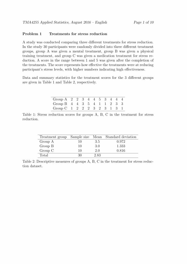
A study was conducted comparing three different treatments for stress reduction.In the study 30 participants were randomly divided into three different treatmentgroups, group A was given a mental treatment, group B was given a physicaltraining treatment, and group C was given a medication treatment for stress re-duction. A score in the range between 1 and 5 was given after the completion ofthe treatments. The score represents how effective the treatments were at reducingparticipant’s stress levels, with higher numbers indicating high effectiveness.

Data and summary statistics for the treatment scores for the 3 different groupsare given in Table 1 and Table 2, respectively.

Group A 2 2 3 4 4 5 3 4 4 4Group B 4 4 3 5 4 1 1 2 3 3Group C 1 2 2 2 3 2 3 1 3 1

Table 1: Stress reduction scores for groups A, B, C in the treatment for stressreduction.

Treatment group Sample size Mean Standard deviationGroup A 10 3.5 0.972Group B 10 3.0 1.333Group C 10 2.0 0.816Total 30 2.83

Table 2: Descriptive measures of groups A, B, C in the treatment for stress reduc-tion dataset.

of 10 TMA4255 Applied Statistics, August 2016 – English

First, it was of interest to compare the mental treatment group (group A) and thephysical training method group (group B).

a) Let SA and SB be the standard deviation from treatment group A and groupB and let them be estimators of σA and σB.Test the hypothesis

H0 : σA = σB vs. H1 : σA 6= σB

by calculating a 95% confidence interval for σA

σB.

Based on the data, can we conclude that the stress reduction scores aredifferent for the two treatment groups (group A and group B)? Write downthe null hypothesis and the alternative hypothesis and perform a two-samplet-test based on the summary statistics in Table 2. Use significance level α =0.05. What are the assumptions you need to make to use this test? What isthe conclusion from the test?

b) A Wilcoxon rank-sum (Mann–Whitney) test was performed on the data forgroup A and B to test if the stress reduction scores are different for the twotreatment groups (group A and group B).Write down the null hypothesis and the alternative hypothesis for this test.From the MINITAB output found in Figure 1, the test statistics isW1 = 116.Show how this value can be obtained from the data in Table 1. Explain brieflyhow the value of W1 is used to test the hypothesis.

Use significance level α = 0.05.

What are the assumptions you need to use this test?Which of the tests in a) (second half) and b) would you consider most ap-propriate for the data? You may base your answer on Figure 2.


Mann-Whitney Test and CI

N MedianGroup A 10 4,000Group B 10 3,000

Point estimate for ETA1-ETA2 is 195,5 Percent CI for ETA1-ETA2 is (-1,000;1,999)W = 116,0Test of ETA1 = ETA2 vs ETA1 not = ETA2 is significant at 0,4274The test is significant at 0,4073 (adjusted for ties)

Figure 1: Printout from Wilcoxon rank-sum test (Mann-Whitney) for the treat-ment for stress reduction dataset.

Figure 2: A normal plot based on the treatment for stress reduction data set, formerged data for group A and group B.


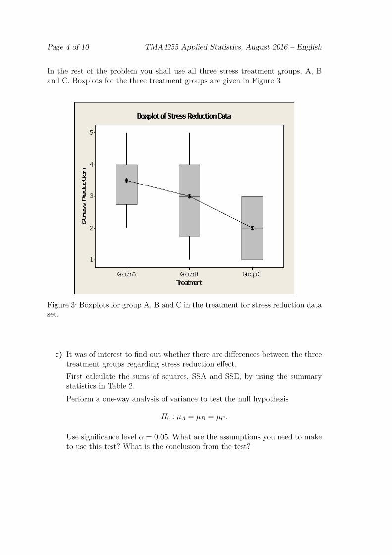
In the rest of the problem you shall use all three stress treatment groups, A, Band C. Boxplots for the three treatment groups are given in Figure 3.

Figure 3: Boxplots for group A, B and C in the treatment for stress reduction dataset.

c) It was of interest to find out whether there are differences between the threetreatment groups regarding stress reduction effect.First calculate the sums of squares, SSA and SSE, by using the summarystatistics in Table 2.Perform a one-way analysis of variance to test the null hypothesis

H0 : µA = µB = µC .

Use significance level α = 0.05. What are the assumptions you need to maketo use this test? What is the conclusion from the test?


d) From the result in c) it was decided to further investigate if any of thedifferences µA − µB, µA − µC and µB − µC are significantly different from 0.Use the Bonferroni method for this problem. The family-wise error rate(FWER), i.e. the probability of making at least one type I error, shouldbe controlled at level α. Use α = 0.05.

Problem 2 Heat flux

Energy engineers are interested in thermal energy from the sun, as part of develop-ment of solar energy. Heat flux is the rate of heat energy transfer through a givensurface per unit time. The heat flux is measured as part of a solar thermal energytest. An engineer is interested in determining how the total heat flux is predictedby the variables: insolation, the position of the east, south, and north focal points,and the time of day. n = 29 thermal energy tests were taken.

The following description is given.

• y: the total heat flux, in kilowatts

• x1: the insolation value, in watts/m2

• x2: the position of the focal point in the east direction, in inches

• x3: the position of the focal point in the south direction, in inches

• x4: the position of the focal point in the north direction, in inches

• x5: the time of day that the data were collected

A pairwise scatter plot and a correlation matrix of the variables are found inFigure 4.


y x1 x2 x3 x4x1 0,628x2 0,102 -0,204x3 0,112 -0,107 -0,329x4 -0,849 -0,634 -0,117 0,287x5 -0,351 -0,584 -0,065 0,697 0,685

Figure 4: Pairwise scatter plots (upper part) and pairwise Pearson correlation(lower part) between variables y, x1, x2, x3, x4 and x5 in the heat flux data set.


A multiple linear regression was fitted to the data with y as response and x1, x2,x3, x4 and x5 as explanatory variables. Let (yi, x1i, x2i, x3i, x4i and x5i) denotethe measurements from the ith thermal energy test, where i = 1, ..., 29. Define thefull model (model A):

Model A yi = β0 + β1x1i + β2x2i + β3x3i + β4x4i + β5x5i + εi, (1)

where εi are i.i.d. N(0, σ2) for i = 1, ..., n. The MINITAB output from a statisticalanalysis of model A is found in Figure 5. Plots of standardized residuals are foundin Figure 6.

Predictor Coef SE Coef T PConstant 325,44 96,13 3,39 0,003Insolation 0,06753 0,02899 2,33 0,029East 2,552 1,248 2,04 0,053South 3,800 1,461 2,60 0,016North -22,949 2,704 -8,49 0,000Time of Day 2,417 1,808 1,34 ?

S = ? R-Sq = ?% R-Sq(adj) = 87,7%

PRESS = 3109,95 R-Sq(pred) = 78,82%

Analysis of VarianceSource DF SS MS F PRegression 5 ? 2639,1 40,84 0,000Residual Error 23 ? 64,6Total 28 14681,9

Figure 5: Printout from fitting linear regression model A for the heat flux dataset.


Figure 6: Residual plots (normal plot based on standardized residuals in the up-per left panel, standardized residual versus fitted values in the upper right panel,histogram based on standardized residuals in lower left panel and standardizedresidual versus observation order in the lower right panel) for linear regressionmodel A in the heat flux data set.


a) Write down the estimated regression equation.

Now turn to the estimated regression coefficient for X5, Time of Day, inthis model. Is the effect of X5, Time of Day, significant in this model?Calculate the R2 and explain how you can interpret this value.What is an appropriate estimate for σ? Give the numerical value of theestimate.Is a significant amount of variation explained by the model? Write down thenull hypothesis and the alternative hypothesis. Choose a test statistics andperform a hypothesis test. Use significance level α = 0.05.

b) Which model assumptions were made in the linear regression model A inEqn.1? Explain and define what a residual is.Figure 6 shows some residual plots for model A. Do the residual plots indicatethat these assumptions for linear regression are satisfied? Justify your answerby commenting briefly on the plots in Figure 6. How should they ideally lookif the model was correct?

We are now interested in comparing different regression models where combinationsof the covariates x1, x2, x3, x4 and x5 are present, in a best subset regression.Assume that an intercept, β0, is present in the regression model.

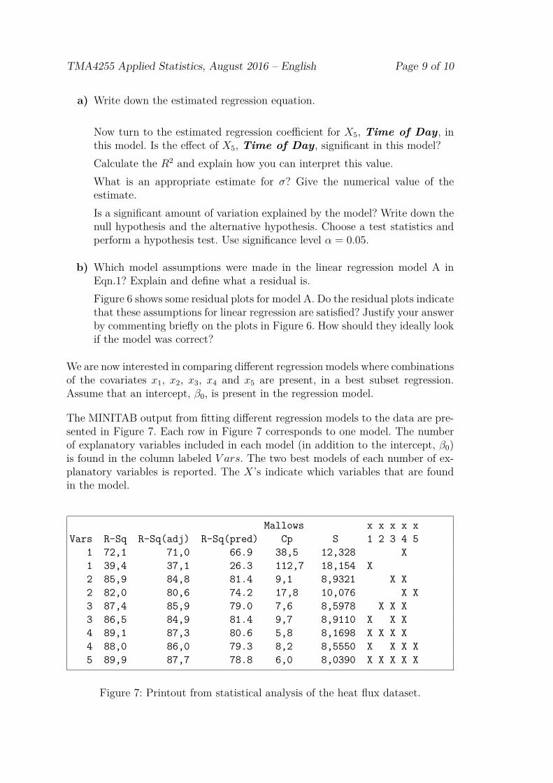
The MINITAB output from fitting different regression models to the data are pre-sented in Figure 7. Each row in Figure 7 corresponds to one model. The numberof explanatory variables included in each model (in addition to the intercept, β0)is found in the column labeled V ars. The two best models of each number of ex-planatory variables is reported. The X’s indicate which variables that are foundin the model.

Mallows x x x x xVars R-Sq R-Sq(adj) R-Sq(pred) Cp S 1 2 3 4 5

1 72,1 71,0 66.9 38,5 12,328 X1 39,4 37,1 26.3 112,7 18,154 X2 85,9 84,8 81.4 9,1 8,9321 X X2 82,0 80,6 74.2 17,8 10,076 X X3 87,4 85,9 79.0 7,6 8,5978 X X X3 86,5 84,9 81.4 9,7 8,9110 X X X4 89,1 87,3 80.6 5,8 8,1698 X X X X4 88,0 86,0 79.3 8,2 8,5550 X X X X5 89,9 87,7 78.8 6,0 8,0390 X X X X X

Figure 7: Printout from statistical analysis of the heat flux dataset.


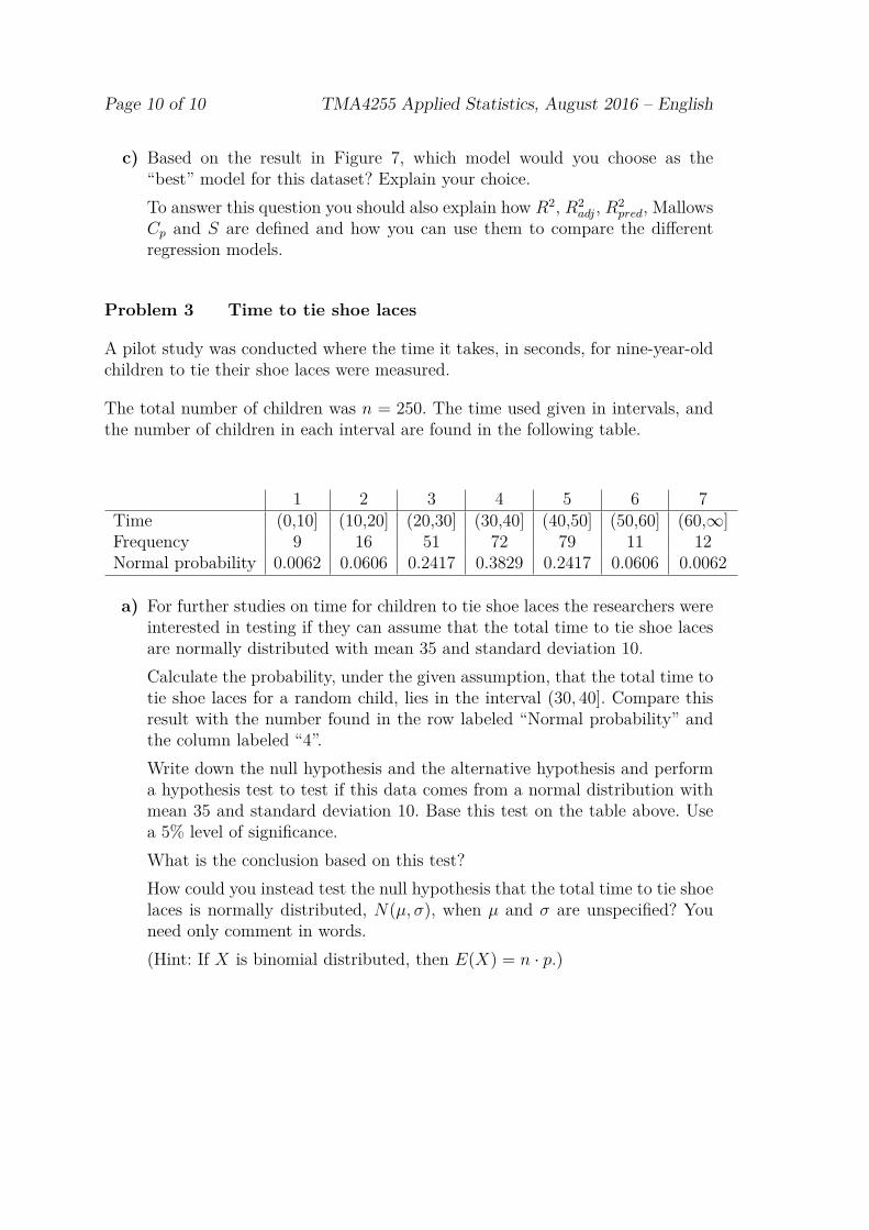
c) Based on the result in Figure 7, which model would you choose as the“best” model for this dataset? Explain your choice.To answer this question you should also explain how R2, R2

adj, R2pred, Mallows

Cp and S are defined and how you can use them to compare the differentregression models.

Problem 3 Time to tie shoe laces

A pilot study was conducted where the time it takes, in seconds, for nine-year-oldchildren to tie their shoe laces were measured.

The total number of children was n = 250. The time used given in intervals, andthe number of children in each interval are found in the following table.

1 2 3 4 5 6 7Time (0,10] (10,20] (20,30] (30,40] (40,50] (50,60] (60,∞]Frequency 9 16 51 72 79 11 12Normal probability 0.0062 0.0606 0.2417 0.3829 0.2417 0.0606 0.0062

a) For further studies on time for children to tie shoe laces the researchers wereinterested in testing if they can assume that the total time to tie shoe lacesare normally distributed with mean 35 and standard deviation 10.Calculate the probability, under the given assumption, that the total time totie shoe laces for a random child, lies in the interval (30, 40]. Compare thisresult with the number found in the row labeled “Normal probability” andthe column labeled “4”.Write down the null hypothesis and the alternative hypothesis and performa hypothesis test to test if this data comes from a normal distribution withmean 35 and standard deviation 10. Base this test on the table above. Usea 5% level of significance.What is the conclusion based on this test?How could you instead test the null hypothesis that the total time to tie shoelaces is normally distributed, N(µ, σ), when µ and σ are unspecified? Youneed only comment in words.(Hint: If X is binomial distributed, then E(X) = n · p.)

examination paper for tma4255 applied statistics · department of mathematical sciences examination...

Documents