DEPARTMENT OF ECONOMICS

ISSN 1441-5429

DISCUSSION PAPER 44/15

Examining Income Convergence among Indian States: Time Series

Evidence with Structural Breaks

Ankita Mishra1 and Vinod Mishra

2*

Abstract: This paper examines the stochastic income convergence hypothesis for seventeen major

states in India for the period from 1960 to 2012. Our panel of states exhibit cross-sectional

dependence and structural breaks in their per capita incomes. By including these two features

in a unified testing framework, we find evidence to support the income convergence

hypothesis for Indian states. The paper also suggests that the failure of other studies to find

evidence of income convergence in Indian states may arise from their not taking into account

potential structural breaks in the income series. Most structural breaks in relative income

correspond to important events in Indian history at the national or regional level.

Keywords: India, panel unit root, structural break, convergence

JEL Classification Numbers: O40, C12

1 School of Economics, Finance and Marketing, RMIT.

2* Department of Economics, Monash University, VIC 3800, Australia. Corresponding Author.

© 2015 Ankita MiMishra and Vinod Mishra

All rights reserved. No part of this paper may be reproduced in any form, or stored in a retrieval system, without the prior

written permission of the author.

monash.edu/ business-economics

ABN 12 377 614 012 CRICOS Provider No. 00008C

3

1. Introduction

Economic growth models based on new growth theory envision poor countries/regions catching up

with rich countries/regions in terms of gross domestic product (GDP)/capita levels (or income per

capita). These economic growth models are based on the belief that economies grow when the capital

per hour worked increases and technological improvements take place. As the pay offs from using

additional capital or better technology are greater for a poor economy, poor economies should be able

to increase their growth rate at a faster rate than richer economies, thus enabling them to catch up.

Various studies in the literature have taken an empirical view as to whether catch up or convergence

has actually occurred for different groups of countries (Mankiw et al., 1992; Evans, 1996, 1997) and

for diverse regions (or states) within a single large country. Studies of the latter have focused

primarily on the United States (Young et al., 2008; Carlino & Mills, 1993). The two main techniques

used to investigate the convergence hypothesis are cross-sectional growth equation estimates (Barro

& Sala-i-Martin, 1992, 1995; Mankiw et al., 1992) and time series unit root testing (Bernard &

Durlauf, 1995; Carlino & Mills, 1993; Fleissig & Strauss, 2001; Strazicich et al., 2004). However,

while the convergence hypothesis has been found to hold true for varied samples of industrial

countries and their regions in cross-sectional studies, time series evidence remains ambiguous

(Strazicich et al., 2004).

The notion of convergence, defined as inclusive growth, holds a pivotal place in Indian central

planning. The ongoing twelfth Five Year Plan (2012‒2017)1 acknowledges that one of the most

important features of growth, relevant for inclusiveness, is a more broad-based sharing of high rates of

economic growth across the states. The draft paper for the twelfth Five Year Plan noted that inter-state

variation in growth rates had fallen compared with the tenth (2002‒2007) and eleventh (2007‒1012)

five year plan periods. Weaker states (Bihar, Orissa, Assam, Rajasthan, Chhattisgarh, Madhya

Pradesh, Uttarakhand, and, to some extent, Uttar Pradesh) were catching up and showed increased

rates of growth. However, imbalances in regional growth remain acute in India. Bandyopadhyay

(2011) has argued that some of the richest states in India (Gujarat and Maharashtra, for example) are

akin to middle income countries, such as Poland and Brazil in their level of development, whereas the

poorest states of Bihar, Uttar Pradesh and Orissa are similar to some of the poorest sub-Saharan

countries in Africa.

1 It is notable that earlier five year plans in India were formulated by an institution called the Planning

Commission. Since January1, 2015, this has been replaced by a new institution, Niti Aayog. In contrast to the

Planning Commission, Niti Aayog is primarily an advisory body with no power to implement policies or

allocate funds. With Niti Aayog, states have been given an active and significant role in the formulation of

economic policies, promoting collective federalism. The approach proposed by Niti Aayog is a bottom-up

approach as opposed to the top-down approach followed by the Planning Commission.

4

Various studies have examined the convergence hypothesis for Indian states. The majority of these

studies has found little support for absolute convergence2 among Indian states; these studies conclude

that there has been increasing divergence in regional per capita income (Marjit & Mitra, 1996; Ghosh

et al., 1998; Nagaraj et al., 2000; Rao et al., 1999; Dasgupta et al., 2000; Sachs et al., 2002; Trivedi,

2002; Shetty, 2003; Bhattacharya & Sakthivel, 2004; Baddeley, 2006; Kar & Sakthivel, 2007;

Nayyar, 2008; Ghosh, 2008, 2010, 2012; Kalra & Sodsriwiboon, 2010). In a few cases, studies have

found evidence in favour of absolute convergence (Dholakia, 1994; Cashin & Sahay, 1996a, 1996b).

Although most studies found evidence against absolute convergence in the per capita incomes of

Indian states, some found support for conditional convergence (Nagaraj et al., 2000; Sachs et al.,

2002; Trivedi, 2002; Baddeley, 2006; Nayyar, 2008; Ghosh, 2008, 2010, 2012; Kalra &

Sodsriwiboon, 2010). In addition, other studies looking at the club convergence hypothesis3 for Indian

states have found limited support in favour of convergence ‒ for example, Baddeley et al. (2006),

Bandyopadhyay (2011) and Ghosh et al. (2013).

Most studies that examine the convergence hypothesis in India are based on a cross-sectional growth

convergence equation approach4 (Bajpai & Sachs, 1996; Cashin & Sahay, 1996; Nagaraj et al., 2000;

Aiyar, 2001; Trivedi, 2002). Very few studies have used stochastic convergence to examine the

income convergence hypothesis for Indian states. These studies are primarily concerned with

identifying the convergence clubs endogenously ‒ see, for example, Chatterjee (1992), Ghosh et al.

(2013) and Bandyopadhyay (2011). In addition, studies using a stochastic convergence approach have

employed different techniques, such as stochastic kernel density techniques in Bandyopadhyay (2011)

or the nonlinear transition factor model in Ghosh et al. (2013). Ghosh (2012) employed the Phillips-

Perron (PP) (Phillips, 1987; Phillips & Perron, 1988) unit root test without structural breaks to

examine the existence of a convergence club in his sample of 15 Indian states. However, none of these

studies has used unit root panel tests with structural breaks to examine the income convergence

hypothesis for Indian states. Many studies, however, have highlighted the shortcoming of previous

time series approaches. Bandyopadhyay (2011), for example, has pointed out that time series

2 The three competing hypotheses on convergence as defined by Galor (1996) are: (1) the absolute convergence

hypothesis, where per capita income of countries (or regions) converge to one another in the long term,

irrespective of their initial conditions; (2) the conditional convergence hypothesis, where per capita income of

countries that are identical in their structural characteristics converge to one another in the long term,

irrespective of their initial conditions; and (3) the club convergence hypothesis, where per capita income of

countries that are identical in their structural characteristics converge to one another in the long term, provided

that their initial conditions are similar. 3 Club convergence entails identifying subsets of states that share the same steady state (or clustering the income

data into convergence clubs) and checking whether convergence holds up within these groups (Ghosh et al.,

2013). In club convergence models, one state is a leading state, known as the leader. All countries with an initial

income gap less than a particular amount (refer to Chatterjee (1992) for details) will eventually catch up with the

leader. In the steady state, all these countries will grow at the same rate and constitute an exclusive convergence

club. 4 For details of this approach, refer to Barro and Sala-i-Martin (1992, 1995), Sala-i-Martin (1996) and Mankiw

et al. (1992).

5

approaches along the lines of Carlino and Mills (1993), which estimate the univariate dynamics of

income, remain incomplete when describing the dynamics of the entire cross section. Ghosh (2013)

has argued that unit root tests employed in stochastic convergence literature are less reliable because

they ignore possible structural breaks in the context of a single time series or in a panel data

framework. Addressing the concerns raised in these studies, this paper employs the latest advances in

the time series approach to examine the stochastic income convergence hypothesis5 among 17 Indian

states in the period from 1960 to 2012. This paper finds evidence to support income convergence

among Indian states, contrary to earlier studies examining regional income convergence in India.

Our paper contributes to the literature on income convergence in India in the following important

ways. First, this testing methodology is not prone to rejections of the null in the presence of a unit root

with break(s), a well-documented criticism laid against traditional univariate unit root tests, such as

the Augmented Dickey Fuller (ADF) and PP tests. In addition, with this approach, the rejection of the

null hypothesis (of a unit root) unambiguously implies stationarity in contrast to earlier uses of unit

root tests with breaks, in which rejection of the null may indicate a unit root with break(s) rather than

a stationary series with break(s). Secondly, this study employs panel versions of unit root tests with

structural breaks that can exploit both the cross-sectional and time series information available in the

data to evaluate the convergence hypothesis, while still allowing for potential structural breaks. Thus,

in a situation in which univariate unit root tests (with or without structural breaks) give conflicting

results, overall income convergence can still be ascertained. Thirdly, cross-sectional dependence is a

potential problem in examining the income convergence hypothesis for states within the same

country. Cross-sectional dependence may arise due to the presence of economy-wide shocks, which

can affect all states (and their income) simultaneously. In order to remove cross-sectional dependence,

the measure of relative per capita income is used (i.e., the per capita income of a particular state

divided by the average per capita income of a group). This type of transformation has been used in

some previous studies to account for cross-sectional dependence, although in a different context ‒ for

example, Meng et al. (2013) in energy consumption, Strazicich and List (2003) in carbon dioxide

emissions, Strazicich et al. (2004) in income convergence among Organisation for Economic

Cooperation and Development (OECD) countries, and Mishra and Smyth (2014) for convergence in

energy consumption among Association of Southeast Asian Nations (ASEAN) countries. This

5 The notion of stochastic convergence implies that shocks to the income of a country (or a region within a

country) relative to the average income of a group of countries (or regions) will be temporary. This entails

testing the null hypothesis of a unit root in the log of the ratio of per capita income relative to the average.

Failure to reject the null of the unit root suggests incomes are diverging and provides evidence against income

convergence. Alternatively, rejection of the null hypothesis of the unit root supports income convergence. Since

the test includes a constant term, stochastic convergence implies that incomes converge to a country- or region-

specific compensating differential. Hence, stochastic convergence is consistent with conditional convergence

(Strazicich et al., 2004).

6

transformation has the advantage that it removes the cross-sectional shocks that affect all the states in

the panel. For example, a positive shock to per capita state domestic product (SDP) across all states

will increase the average by the same proportion and hence leave the relative per capita GDP series

unchanged. This suggests that any structural breaks identified in the transformed series should be state

specific. In our case, this measure of relative per capita income also exhibits cross-sectional

dependence. Therefore, we apply a cross-sectionally dependent unit root test and its panel counterpart

(CIPS test) as proposed by Pesaran (2007). This takes specific account of the cross-sectional

dependence present in the data. However, we note that our panel of states exhibits cross-sectional

dependence along with the existence of structural breaks. In such a scenario, the income convergence

hypothesis cannot be assessed unless we use a method that can simultaneously take into account both

factors. Keeping this in mind, we applied the Bai and Carrion-i-Silvestre (2009) panel unit root test,

which includes possible cross-sectional dependence and structural breaks in a unified framework.

The rest of the paper is organised as follows. Section 2 outlines the econometric methodology.

Sections 3 and 4 describes the data and present the results. Section 5 discusses the results and Section

6 presents the conclusions.

2. Econometric methodology

2. 1 Conventional unit root tests

To start with, this paper employs conventional univariate unit root testing methods without structural

breaks. The rationale behind applying these three conventional tests is to use them as a benchmark

against which to compare the respective test versions that include structural breaks. The comparison

between these two sets of results helps to identify the extent to which misspecification is due to

ignoring structural breaks.

The conventional univariate unit root tests that we employ are the ADF (Dickey & Fuller, 1979), the

Kwiatkowski-Phillips-Schmidt-Shin (KPSS) stationarity test (Kwiatkowski et al., 1992) and the

Lagrange multiplier (LM) unit root test proposed by Schmidt and Phillips (1992). The null hypothesis

for the ADF and LM unit root tests is that the per capita income series of state 𝑖 contains a unit root. If

the null of a unit root is accepted for the per capita income series of state 𝑖, this implies that shocks to

the income of state 𝑖 relative to the average income (measured by per capita income at the state

level) will be permanent. Hence, the per capita income of state 𝑖 will diverge from national per capita

income. On the contrary, if the null hypothesis of a unit root in the per capita income series of state

𝑖 is rejected, this suggests that shocks to the income of state 𝑖 relative to national per capita income

will be temporary; over the long term, the per capita income of state 𝑖 will converge to the average per

7

capita income of the group. The KPSS test differs from these two tests in its null hypothesis. The

KPSS test has the null hypothesis of (trend) stationarity against the alternative hypothesis of unit root.

As these tests are well documented in the literature, we do not discuss the full scope, methodology

and limitations of these tests here6.

2.2 Cross-sectional dependence

An important issue in the context of this analysis is cross-sectional dependence. As the states lie

within a single monetary and fiscal regime and share a high degree of economic and cultural

commonality, we anticipate an element of cross-sectional dependence in per capita incomes. As

suggested in Mishra, Sharma and Smyth (2009), cross-sectional dependence can create large

distortions in conventional univariate and panel unit root tests. Transforming the series to the natural

logarithm of the relative per capita series can remove the cross-sectional dependence to an extent.

To test the effectiveness of the transformation of per capita income series into to relative per capita

income series in removing cross-sectional dependence, Pesaran’s (2007) cross-sectional dependence

(CD) test was conducted before and after transforming the per capita income series into relative per

capita net state domestic product (NSDP). The Pesaran (2007) CD test is based on performing

individual ADF(P) regressions for lags 1 to 4 and collecting the regression residuals to calculate the

pair-wise cross-sectional correlation coefficients of the residuals (denoted by 𝜌𝑖𝑗). A simple average

of these correlation coefficients (��) and the associated CD statistic follow an 𝑁(0,1) distribution. The

null hypothesis in the CD test is that the series are cross-sectionally independent. However, if cross-

sectional dependence is found to be present in the data, Pesaran (2007) proposes an additional cross-

sectionally dependent unit root test and its panel counterpart (CIPS), which specifically takes cross-

sectional dependence into account. The null hypothesis of the CIPS test is unit root, after accounting

for cross-sectional dependence in the data.

2.3 Univariate unit root tests with two structural breaks

Another potential problem with conventional unit root tests and cross-sectional dependence tests is

that these tests do not take into account the possibility of structural breaks in data series. As a result,

the ability of these tests to reject the null hypothesis of unit root declines where data series contain

structural breaks (Perron, 1989). Many significant events have occurred in the Indian economy during

the period 1960‒2012, giving rise to the possibility of breaks in the trend rate of growth of the per

capita income of Indian states. Therefore, ignoring the possibility of structural breaks in the income

series of Indian states could lead to erroneous results.

6 For details, refer to Smyth, Nielsen and Mishra (2009).

8

This paper uses the LM unit root test of Lee and Strazicich (2003) and the KPSS unit root test of

Carrion-i-Silvestre and Sansó (2007) with two endogenous breaks. The LM unit root test has the

advantage over ADF-type endogenous break tests (Zivot & Andrews, 1992; Lumsdaine & Papell,

1997) in that it is unaffected by breaks under the null of a unit root. In ADF-type endogenous break

unit root tests, the critical values are derived assuming no break(s) under the null. As a result, in ADF-

type endogenous break unit root tests, it is possible to conclude that a data series is trend stationary

when in reality it is non-stationary with breaks. This can give rise to a spurious rejection problem (Lee

& Strazicich, 2003).

Lee and Strazicich (2003) developed two versions of the LM unit root test with two structural breaks.

This paper applies the Model CC specification, which can accommodate two breaks in the intercept

and the slope7. The test relies on determining the breaks where the endogenous two-break LM t-test

statistic is at a minimum. Critical values for this case are tabulated in Lee and Strazicich (2003).

The other univariate unit root test used in this paper is the KPSS stationarity test of Carrion-i-Silvestre

and Sansó (2007) with two endogenous breaks in the intercept and trend. This test is the equivalent of

a KPSS test with two structural breaks. The null hypothesis is stationarity with structural breaks. In

the current application of this test, we used the Bartlett kernel and selected the bandwidth using

Andrew’s method8. The break dates are estimated by minimising the sequence of the sum of squared

residuals (SSR) proposed by Kurozumi (2002). This procedure chooses the dates of the breaks from

the argument that minimises the sequence of 𝑆𝑆𝑅(𝑇𝐵1, 𝑇𝐵2), where the SSR is obtained from the

regression of 𝑦𝑡 = 𝑓(𝑡, 𝑇𝐵1, 𝑇𝐵2) + 𝑒𝑡, such that 𝑓(𝑡, 𝑇𝐵1, 𝑇𝐵2) denotes the determining

specification.

2.4 Panel unit root tests with structural breaks

This paper implements the panel KPSS stationarity test with multiple breaks (Carrion-i-Silvestre et

al., 2005). This test has the null of stationarity and hence takes into account the criticism by Bai and

Ng (2004) that for many economic applications it is more natural to take stationarity rather than non-

stationarity as the null hypothesis. It allows for structural shifts in the trend of the individual time

series in the panel and permits each state in the panel to have a different number of breaks at different

dates. This has the advantage that it allows the most general specification in which each state’s

relative per capita series can be modelled independently with its own structural breaks caused by

state-specific shocks. In addition to the panel test statistic, the KPSS stationarity test (Carrion-i-

Silvestre et al., 2005) produces results for individual time series in the panel. This has the advantage

7 For other versions and more technical details of the test, refer to Smyth, Nielsen and Mishra (2009).

8 While the results as reported in this paper use the Bartlett kernel, they were also estimated using the quadratic

kernel. The results were not sensitive to the choice of kernel.

9

of relating an important event in the history of a particular state back to the break dates identified by

the test. In addition, it allows different states to have different numbers of structural breaks.

The Carrion-i-Silvestre et al. (2005) KPSS test is a generalisation for the case of multiple changes in

the level and slope of Hadri’s panel stationarity test (2000), which is computed as the average of

univariate KPSS stationarity tests. The distinguishing feature of this test is that it only produces

statistically significant breaks. To estimate the break dates, Carrion-i-Silvestre et al. (2005) apply the

Bai and Perron (1998) technique. Trimming is necessary when computing estimates of break dates.

The trimming region used here is ]9.0,1.0[T . Once all possible dates are identified, Carrion-i-

Silvestre et al. (2005) recommend that the optimal break dates are selected using the modified

Schwartz information criterion (SIC) (Liu et al., 1997) for trending regressors. This method involves

sequential computation and the detection of breaks using a pseudo F-type test statistic. The Carrion-i-

Silvestre et al. (2005) test allows for a maximum of five structural breaks.

In addition to the Carrion-i-Silvestre et al. (2005) test, this paper also computes panel LM unit root

tests with structural breaks (Im et al., 2005) as a robustness check. Unlike the Carrion-i-Silvestre et al.

(2005) test, this test has the null hypothesis of panel unit root, which suggests that the per capita

incomes of Indian states are not converging.

Finally, we estimated the results of the Bai and Carrion-i-Silvestre (2009) panel unit root test, which

includes possible cross-sectional dependence and structural breaks in a unified framework. The

methodology proposed in this paper relies on modelling the cross-sectional dependence as a common

factors model, as described in Bai and Ng (2004) and Moon and Perron (2004). The purpose of using

common factors is to distinguish between the co-movements and idiosyncratic shocks that may affect

individual time series. Once the time series are filtered for co-movements, the cross-sectional

correlation is sufficiently reduced and one can expect to derive valid panel data statistics.

The Bai and Carrion-i-Silvestre (2009) panel unit root test allows the common factors to be a non-

stationary 𝐼(1) process, a stationary 𝐼(0) process or a combination of both. The advantage of this

approach is that it allows common shocks to have different impacts on individuals via heterogeneous

factor loadings. As the number and location of structural breaks are unknown and the common and

idiosyncratic factors are typically unobservable, this paper develops an iterative estimation procedure

for handling the heterogeneous break points in the determining components. The algorithm of this

iterative procedure is detailed in Bai and Carrion-i-Silvestre (2009). After estimating the location of

breaks, common factors, factor loadings and the magnitude of changes, modified Sargan-Bhargava

(MSB) statistics are calculated for each series. Finally the individual MSB statistics are pooled to

10

construct the panel MSB. Based on the method used for pooling the individual statistics, Bai and

Carrion-i-Silvestre (2009) suggest two types of panel MSB statistics: standardised statistics or a

combination of P-values. As suggested in the paper, standardised statistics are best suited for our

purposes. Although this paper proposes a relatively complicated model with both cross-sectional

dependence and structural breaks modelled simultaneously in one framework, this model is closest to

the empirical settings of the current paper.

3. Data

The data used are the per capita net state domestic product (NSDP) for 17 major Indian states for the

period from 1960 to 2012. Data were collected from the Indiastat database. The NSPDs for the 17

major states were expressed in Indian Rupees (INRs) and provided at different base periods. All the

series were converted to the common base period of 2004‒20059. The 17 major states included in our

analysis account for roughly 90% of India’s population and make up around 87% of India’s GDP. The

remaining 11 states10

, not included in the analysis, were either created very late in the period of

analysis (such as Chhattisgarh, Jharkhand and Uttrakhand), were too small with lots of missing data

points (Goa, Mizoram, Sikkim, Arunanchal Pradesh, Maghalya and Himanchal Pradesh, for example),

or had unreliable data points (Jammu, Kashmir and Nagaland, for example). It is a common practise

in studies looking at state-level analysis in India to focus on 15 to 17 major states. Refer to Table 3.1

in Ghosh (2013).

Descriptive statistics on NSDP per capita are reported for the full sample period in Table 1. More than

half of the states (nine out of seventeen) have average annual per capita income below INR 10,000

(US$ 227)11

with Bihar (preceded by Uttar Pradesh, Assam, Madhya Pradesh, Orissa, Manipur,

Rajasthan, Tripura and West Bengal) at the bottom of the list. Three states (Haryana, Maharashtra and

Punjab) have average annual per capita income above INR 15,000 (US$ 341) and the remaining five

states (Gujarat, Tamil Nadu, Kerala, Karnataka and Andhra Pradesh) have average annual per capita

income between INR 10,000‒15,000 for the period from 1960 to 2012. Fluctuations in per capita

income around the mean (as measured by standard deviation) are in line with the ranking of states on

income. Haryana displays the highest fluctuations with Bihar showing the lowest variations. NSDP

per capita series for all the states are positively skewed indicating that the future values of NSDP per

capita are more likely to be higher than the mean.

9 The latest base period used for compiling the net state domestic products.

10 The Republic of India, as of writing this paper, is made up of 29 states and 6 union territories. However, one

state (Telangana) was carved out of Andhra Pradesh in 2014. As the period of analysis for this study concludes

in 2012, Telangana is not treated independently but is viewed as part of Andhra Pradesh. 11

The average annual exchange rate between the Indian rupee and the US dollar during 2004‒05 was 1 US$ =

44 INR.

11

INSERT TABLE 1 HERE

This paper has taken the relative per capita income measure to examine the convergence hypothesis.

For this, the NSDP per capita of state 𝑖 is converted to its relative NSDP per capita in the following

way:

𝑅𝑒𝑙𝑎𝑡𝑖𝑣𝑒 𝑃𝑒𝑟 𝐶𝑎𝑝𝑖𝑡𝑎 𝑁𝑆𝐷𝑃𝑖𝑡 = 𝑙𝑛 (𝑃𝑒𝑟𝐶𝑎𝑝𝑖𝑡𝑎 𝑁𝑆𝐷𝑃𝑖𝑡

𝑁𝑎𝑡𝑖𝑜𝑛𝑎𝑙 𝑃𝑒𝑟 𝐶𝑎𝑝𝑖𝑡𝑎 𝐼𝑛𝑐𝑜𝑚𝑒𝑡)

Panel B of Table 1 presents the descriptive statistics of the relative series of per capita income of state

i/national per capita income. In a hypothetical scenario, where the per capita income of a state is

exactly equal to the national per capita income, this series will take a value of one, whereas a value

smaller than one would mean that the per capita income of that state is less than the national average.

A value greater than one would indicate that the per capita income of the state is higher than national

per capita income. We note that the per capita income of the poorer states, such as Bihar, Uttar

Pradesh and Orissa, are much lower than one, whereas some of the rich states, such as Haryana,

Punjab, Gujarat and Maharashtra, are much higher than one.

The entire analysis was conducted on the natural logarithm of this transformed series. The natural

logarithm of this relative series means that in the hypothetical scenario where a state’s per capita

income is exactly equal to the national per capita income, it would take a value of zero. If relative per

capita NSDP is found to be stationary, this would mean that the per capita income of the state is not

drifting uncontrollably away from the national average. Any state-specific shocks (such as natural

disasters, political turmoil or civil unrest) have only a temporary affect and the per capita series

eventually reverts to the national average. If most or all of the per capita income series are found to be

stationary around the national average, it would mean that the income convergence hypothesis would

hold true for Indian states over the long term. On the contrary, finding a unit root (or non-stationarity)

for most of the series would provide evidence in support of the non-convergence hypothesis.

Figure 1 presents the time series plot of the natural logarithm of the relative NSDP series for each

state. The horizontal line at zero indicates the hypothetical scenario in which state per capita income is

the same as national per capita income (i.e. perfect convergence). A primary examination of the plot

for each state reveals that we can categorise the states into three distinct categories: namely, states that

stayed above the national average throughout the sample period (rich states); states that stayed below

the national average throughout the sample period (poor states); and states that moved above and

below the national average (swing states). The first category comprises Gujarat, Maharashtra and

Punjab. The states of Haryana and Kerala are below the national average at the beginning of the

12

sample. However, fairly early in the analysis period, income moves above the national average and

remains above average for the rest of the analysis period. The second category comprises Uttar

Pradesh, Bihar, Orissa and Madhya Pradesh. These states remain below the national average

throughout the analysis period. The rest of the states (eight in total) fall into the category of swing

states.

4. Results

As a benchmarking exercise, the ADF, the Schmidt and Phillips LM unit root test and the KPSS

stationarity test without structural breaks were carried out. The results for these tests are reported in

Table 2. The results for the ADF test suggest that the null of unit root cannot be rejected in any of the

transformed series at the traditional levels of significance. This test gives no evidence of convergence

in per capita incomes. In the KPSS test, the null of stationarity is rejected for 11 out of 17 series. The

Schmidt and Phillips LM test fails to reject null of unit root in 12 out of 17 cases. On the basis of the

univariate unit root tests without structural breaks we can conclude that between zero and seven states

are converging towards national average per capita income.

INSERT TABLE 2 HERE

The results for the test of cross-sectional independence are reported in Table 3. The top panel reports

the results for the untransformed series. The Pesaran CD statistic is highly significant at all four lags,

implying clear rejection of the null of cross-sectional independence. The bottom panel reports CD

statistics for the transformed series. Although the absolute value of the CD statistics has reduced after

transformation, the null hypothesis of cross-sectional independence is still rejected at the 1% level.

Thus, transforming the series is not enough to remove the cross-sectional dependence in our sample

and there is a need to conduct a CIPS unit root test, which specifically takes into account this cross-

sectional dependence.

INSERT TABLE 3 HERE

The results of Pesaran (2007) CIPS unit root test are reported in Table 4. The results of individual

CIPS unit root tests suggest a failure to reject null of unit root for most states. We note that the null of

unit root is rejected at the 5% level or better for 6 states at lag 1, is rejected for only 2 states at lag 2,

and for none at lags 3 and 4. The overall conclusion based on these tests results is that there is no

indication of convergence in per capita incomes for most of the Indian states in the sample. The

results are similar to those obtained using the traditional unit root test: between zero and six states

13

seem to be converging towards national average per capita income. Even though the CIPS test

accounts for cross-sectional dependence, there is still a possibility of specification bias due to

unaccounted structural breaks in the series. As a result, we now move to the tests that specifically

account for structural breaks in the data.

INSERT TABLE 4 HERE

Table 5 presents the LM unit root test results and the results of the KPSS stationarity test with two

endogenous breaks in the intercept and slope. The Lee and Strazicich (2003) LM unit root test is an

LM test with a null hypothesis of unit root in the series. Model CC, the most general specification of

the test was used. This allows for two breaks in the intercept as well as trend of the series. In this test,

the null hypothesis of a unit root was rejected by looking at the LM parameter. The presence of

significant structural breaks was determined by looking at the significance of the dummies for breaks

in intercept and trend. The full results of this test include the LM test statistics, the coefficients, and

the significance of dummies for breaks in trend and intercepts for the break dates that were

endogenously determined by the test. In Table 4, however, only the LM test statistics and the break

dates identified by the test are reported. In terms of the significance of the break dates, the results

suggest that in most of cases, both the dummies (break in intercept and break in trend) were

significant and at least one dummy was significant at each break date reported. After taking into

account the occurrence of structural breaks in the series, the null of a unit root in the relative per

capita NSDP series was rejected for 11 states (64.8% of the sample) at the 5% level of significance or

better and 13 states (76.5% of the sample) at the 10% level or higher. Comparing these results with

those reported in Column 3 of Table 2 (the Schmidt and Philips LM unit root test), it can be noted that

the number of states for which the null of unit root can be rejected increases dramatically where

structural breaks were excluded from the data (13 out of 17 states as compared with 5 out of 17).

The second test presented in this table is the Silvestere and Sanso (2007) KPSS test with two

structural breaks. Based on the KPSS test, this test allows for two breaks in the series and has a null

hypothesis of stationarity. It uses the Bayesian information criterion (BIC) to select the two significant

breaks over the entire set of break-point combinations. The results of this test were compared with the

KPSS test results reported in Table 2, Column 2. The KPSS test uses the same methodology but does

not allow for structural breaks in the data. The results of this test support the convergence hypothesis

more strongly. The KPSS test fails to reject the null hypothesis of stationarity for 12 states (70.5% of

the sample) at the 5% level and for 13 states (76.5% of the sample) at the 10% level or higher.

INSERT TABLE 5 HERE

14

The results of individual states for the Carrion-i-Silvestre et al. (2005) KPSS unit root test are reported

in Table 6. This test was conducted allowing a maximum of five structural breaks in the intercept and

trend of each state’s series. However, not every state had five significant structural breaks in the

relative per capita NSDP series. For most of the states, around three to four structural breaks were

found to be significant. Table 6 reports only the significant structural breaks. Even after accounting

for up to five structural breaks, the null of stationarity is still found to be rejected in five out of

seventeen states.

INSERT TABLE 6 HERE

These test results point to considerable, though not universal, evidence of convergence in the per

capita income of different Indian states. After accounting for structural breaks in the individual

relative income series, most states exhibit convergence towards the national average in per capita

NSDP. However, for few states, convergence of income does not hold true. Therefore, the next logical

step was to check the stationarity of the overall panel of the relative incomes of Indian states.

Stationarity of the whole panel would suggest that the overall evidence in favour of convergence of

incomes outweighs the evidence against convergence.

Table 7 reports the panel unit root test results for the Hadri (2000) test (without structural breaks), the

Carrion-i-Silvestre et al. (2005) test (with a maximum of five structural breaks), the Im et al. (2005)

LM unit root test (with zero, one and two structural breaks) and the Pesaran (2007) CIPS test. The

Hadri (2000) and Carrion-i-Silvestre et al. (2005) tests are reported with two alternative assumptions:

namely, that that the long-term variance was homogeneous or was heterogeneous. The null hypothesis

of stationarity was not rejected in any of the cases, which implies that there is strong evidence of

mean-reversion in the panel of relative incomes. This result is robust with regard to the alternative

assumptions about the variance and the presence/number of structural breaks in the data. These results

were confirmed by the panel LM unit root test (Im et al., 2005), reported in Panel C of Table 7. The

null hypothesis in this case is a unit root; the test was conducted with alternate specifications of zero,

one and two structural breaks in the individual data series. The null hypothesis of unit root was

rejected at traditional levels of significance in all the specifications, suggesting strong evidence of

convergence in per-capita incomes for the overall panel. The results of the Pesaran (2007) CIPS tests

remain inconclusive with regard to the convergence hypothesis at the overall panel level. The null

hypothesis of a unit root was rejected for two lags, but was accepted for the remaining two lags at a

5% level of significance.

An overall view of the results obtained so far suggests the tests with structural breaks (i.e., that ignore

cross sectional dependence) show evidence for convergence, whereas the tests that account for cross-

15

sectional dependence (but ignore structural breaks) fail to find evidence in support of convergence. To

resolve this apparent contradiction, we used the Bai and Carrion-i-Silvestere (2009) test, which

simultaneously takes into account possible cross-sectional dependence and multiple endogenous

structural breaks. This test produced two sets of three statistics, of which 𝑃𝑚∗ is the most suitable for

large N panels. Panel D of Table 7 reports the results of the Bai and Carrion-i-Silvestre (2009) test for

the overall panel. We note that all three test statistics reject the null of unit root, suggesting income

convergence among Indian states, when controlling for both cross-sectional dependence and structural

breaks.

INSERT TABLE 7 HERE

5. Discussion

The results of this study raise two questions for discussion: first, whether or not we find evidence

supporting per capita income convergence among Indian states, and secondly, what are the dates of

the structural breaks identified by our tests and do they actually correspond with major events

affecting the Indian economy. We begin by considering the issue of convergence.

5.1 Evidence for convergence

As discussed earlier, the stationarity of relative per capita NSDP seems to indicate that a state is

converging towards national average per capita income. The results presented in Table 7 for the

overall panel indicate that the evidence in support of the convergence hypothesis outweighs support

against the hypothesis. From the evidence presented in Tables 3, 4, 5 and 6 we know that not all the

individual states are converging towards the national average in the long term. However, the majority

of states are converging (around 70% of the sample). Therefore, the panel unit root test results suggest

overall convergence.

Looking at the individual states and contrasting Tables 3 and 4 with Tables 5 and 6, we can conclude

that the evidence for or against convergence is contingent upon how we decide to model the data. Any

model that does not take into account the structural breaks in the series will not find convergence in

per capita incomes. The same unit root tests (i.e., KPSS and LM tests) give a non-stationary result for

most of the series when structural breaks are not included (Table 3). However, when two structural

breaks are taken into account (Table 5), the tests detect stationarity (for most of the series). The states

which do not conform to the convergence hypothesis also vary depending on the unit root test used.

Using the LM test with two structural breaks, we find that Assam, Maharashtra, Tamil Nadu and Uttar

Pradesh are not converging towards national per capita GDP, whereas, when the null of stationarity is

16

used in the Silvestere and Sanso (2007) KPSS test with two structural breaks, we find that the states

which are not converging to the national average are Gujarat, Haryana, Orissa, Tripura and West

Bengal. The states identified as non-converging in the long term are not the same under the two tests.

The fact that the stationarity hypothesis is rejected for few states in each test is probably due to the

way a particular test models the data generating process.

Of particular interest are the results for the individual states in the panel KPSS test, presented in Table

6. This test allows for the maximum of five structural breaks in the trend and intercept of the relative

per capita income series. Only the significant breaks are reported. We expected this test to suffer least

from any possible misspecification bias in the structural breaks, as the possibility of ignoring

structural breaks is minimised by allowing five breaks. If anything, there is a possibility of over-fitting

the data by allowing too many structural breaks, which would bias our results in favour of

convergence. However, as reported in Table 6, we do not find any stronger evidence for the

convergence hypothesis using this test than for the tests with two structural breaks. This test suggests

that five states, namely, Andhra Pradesh, Assam, Manipur, Punjab and Uttar Pradesh are not

converging towards the national average. With the exception of Uttar Pradesh and Assam, which are

also identified as non-converging in the LM test with two structural breaks, none of the remaining

three states are identified as non-converging in any of the previous tests, which used a different

assumption for generating data and imposed a different number of structural breaks. The results

indicate substantial support for the convergence hypothesis, irrespective of the methodology used.

In summary, we used three tests of stationarity that do not allow for structural breaks in the series and

three tests that allow for structural breaks. We used the following rule of thumb to decide an overall

result in each category: ‘If two out of three tests in a particular category suggest stationarity, we then

categorise the series as stationary. Otherwise it is non-stationary’.

Based on this rule of thumb, all the states except Gujarat, Kerala, Rajasthan and West Bengal are non-

stationary when we do not allow for structural breaks, whereas only the states of Assam and Uttar

Pradesh are found to be non-stationary when we allow for two or more structural breaks in the series.

To decide between the conflicting stationarity and non-stationarity results, we took the result obtained

from the model with structural breaks as the final result. Tests that allow for structural breaks assumed

more parameters in the data generating process and hence provide a better fit to the data. Also, given

the time series of the last five decades, it seemed natural to rely on the model with structural breaks.

Using this decision rule, we concluded that only the states of Assam and Uttar Pradesh are non-

stationary, i.e., do not conform to the convergence hypothesis. The most probable reason for this

seems to be political rather than economic. Both states have experienced long periods of political and

social unrest, accompanied by either no normal government (presidential rule) or by short-lived and

17

dysfunctional governments. This conclusion is supported by the fact that the break dates in these

states match major socio-political events. We discuss the location of break dates and the possible

events to which they correspond in a later section of this paper.

Table 7 presents the overall verdict in terms of panel unit root tests. Here, we note that all three panel

unit root tests suggest convergence in per capita incomes. The panel version of the Pesaran (2007) test

confirms the convergence hypothesis for three out of four lags, despite the fact that the univariate

version of the same test fails to confirm the convergence hypothesis for most of the states. The Hadri

(2000) panel KPSS test without structural breaks and the Carrion-i-Silvestere et al. (2005) panel

KPSS test with multiple structural breaks both confirm the convergence hypothesis for the overall

panel (by failing to reject the null of stationarity), irrespective of whether we assume the long-term

variance to be homogeneous or heterogeneous. The same story is reaffirmed by the panel version of

the LM test (Im et al., 2005), which strongly rejects the null of unit root, irrespective of the number of

structural breaks allowed in the series.

The results endorse the success of India’s central planning in achieving the objective of inclusive

growth over the last five decades. Despite the fact that there are strong differences between the per

capita incomes of the states, they all appear to have benefited from economic growth and incomes are

converging towards the national average. A particularly encouraging element of this analysis is that

the low-income states are catching up with the high-income states, suggesting that regional disparities

in per capita income will not persist in the long term.

5.2 Structural breaks

The presence of structural breaks carries significant implications for our findings. As pointed out by

Strazicich et al. (2004), the accurate detection of these structural breaks increases the ability to reject

the null hypothesis of unit root. State-specific conditioning variables, such as physical

infrastructure/investment expenditure (as measured by irrigation, electrification and railway track-

building expenditure in Bandyopadhyay (2011) or Baddeley et al. (2006)) and social infrastructure

(defined as human capital in Lahiri et al. (2009)) can be permanently altered following a major shock,

making permanent changes to the time path of relative income. Ignoring these structural breaks in the

analysis seems the reason that earlier studies on state income convergence in India could not find

evidence of stochastic convergence.

In this section, we explore whether the identified structural breaks can be linked to significant

political, economic and environmental events that occurred regionally or nationally in India.

Structural breaks are distributed across the entire period of five decades covered in our study. Not

18

surprisingly, given the number of states in India, the total number of state-level shocks is high. In the

following paragraphs, we discuss major national events and the timing of structural breaks in different

states.

For the majority of states, with the exception of Bihar, Gujarat and Tripura, the first and second

structural breaks in relative income occurred during the period from 1966 to 1979. This period is

characterised by a number of major economic upheavals. India experienced three economic crises

during the period, one in 1965‒66 (the period in which most of the first structural breaks occur), a

second in 1973‒74 and a third in 1979‒80 (the period when a second structural break was

encountered in most states). All three crises were predominantly balance of payment crises, which

were caused by a shortage of food crops triggered by droughts and further aggravated by external

factors such wars (with Pakistan in 1965 and 1971) and the international oil crises of 1973 and 1979.

Many states experienced a structural break in the mid to late 1980s. These include Andhra Pradesh

(1986), Assam (1984), Bihar (1983‒84), Gujarat (1984), Kerala, Madhya Pradesh, Manipur, Tripura

and West-Bengal in the period 1985‒87. This period was also marked by several significant political

and economic incidents in India. Following a tumultuous period from 1965 to 1980, the Indian

economy witnessed a turnaround and experienced high growth in the 1980s. However, this period of

development was also characterised by an unsustainable level of government spending, resulting in

mounting internal and external debt and expenditure on subsidies giving rise to a severe balance of

payments crisis in India in 1991. On the socio-political front too, this period was turbulent, with many

dramatic changes that may have had varying levels of instantaneous or delayed impact on different

states. In 1984, after the assassination of the then Prime Minister, Indira Gandhi, communal riots

broke out in New Delhi and in most of northern India, which led to the massacre of around 5,000

citizens of the Sikh faith in Delhi, Kanpur and other cities. The same year, 1984, also witnessed the

world’s worst industrial disaster in terms of the human lives effected. On December 3, 1984, in

Bhopal, the capital city of the central state of Madhya Pradesh, a chemicals manufacturing company

(Union Carbide Corporation) released methyl isocyanate (MIC) into the atmosphere above Bhopal.

The leak was due to employer negligence and poor plant maintenance. Officially, the state

government put the death toll at around 4,000; however, unofficial estimates say it killed 20,000 and

injured over 500,000 people, making it the world’s worst industrial disaster. The insurgency in the

state of Jammu and Kashmir (not included in this analysis) took an ugly turn in 1989 with the exodus

of Kashmiri Pandits (members of a minority Hindu community in Kashmir valley) and the targeted

killing of key community figures. In a relatively short space of time, close to 75,000 Kashmiri Pandit

families were forced to flee Kashmir and seek refuge in other north Indian states. This had

considerable impact on the resources and socio-political dynamics of many neighbouring states

including the Union Territory of Delhi (not included in the analysis).

19

With the exception of Haryana, Madhya Pradesh, Orissa and Tamil Nadu, all the states experienced a

structural break at some point between 1991 and 1995. This decade too was very significant in the

Indian economy. Many of the economic and policy decisions taken during this period are still shaping

the growth trajectory of the Indian economy. The decade started with the continuation of balance of

payments problems, which India had experienced since 1985. The Iraqi invasion of Kuwait in August

1990 resulted in a sharp increase in the international price of oil, which further worsened the problem

and, by the end of 1990, the Indian economy witnessed a very acute macroeconomic crisis. The

government was close to default, its central bank had refused new credit and foreign exchange

reserves had been reduced to such a point that India could barely finance three weeks’ worth of

imports. After securing a loan of $US 2.2 billion from the IMF (pledging 67 tons of India’s gold

reserves as collateral), the Indian government initiated a major programme of structural and economic

reform in 1991 under the supervision of the then finance minister, Manmohan Singh, bringing about

significant policy changes in the external, financial and industrial sectors. Singh later served as prime

minister of India from 2004 to 2014.

On the political front, ex-prime minister Rajiv Gandhi was assassinated in May 1991 by the

Liberation Tigers of Tamil Elam (LTTE), a militant organisation from Sri Lanka. The Indian

economy experienced a period of political uncertainty from 1996 to 1999, with three general elections

in three years. India also faced a brief period of war with Pakistan in 1999, known as the Kargil War,

and short-lived economic sanctions by United States as a fall out from nuclear tests in 1998. This

period of political turmoil and uncertainty ended in 1999 when the National Democratic Alliance

(NDA), a coalition of 20 parties headed by the Bharatiya Janata Party (BJP), managed to secure a

majority and formed a government that completed its full term.

In addition to the national events described above, many state-specific events/developments took

place during the period. This can be used to explain the existence of structural breaks in the income

series of a particular state that do not match any national event. Table 8 lists the state-specific events

that occurred around the break dates. These state-specific events justify the existence of breaks in the

income series from that time onward.

INSERT TABLE 8 HERE

5.2.1 Case study of Uttar Pradesh and Assam

The discussion in the previous section provides ample evidence to support the existence of structural

breaks in the relative per capita income of Indian states. This further highlights that tests which

specifically take into account the existence of structural breaks are more credible and produce

20

unbiased results. As noted earlier, given the three different types of unit root tests with structural

breaks that we applied in this paper, if we follow the rule of thumb and consider the relative income

of a state to be stationary (or converging) if the majority of the tests (two out of three) suggest

stationarity or convergence, we discover that there are only two states for which convergence to the

national average does not hold true. These states are Uttar Pradesh and Assam. In the paragraphs

below, we will attempt a critical analysis of events that occurred in these states to find out the possible

reasons why these states are lagging behind and do not seem to be converging towards the national

average.

Uttar Pradesh is the most populous and one of the poorest states of India. Panel B of Figure 2 depicts

the breaks in the relative per capita series for Uttar Pradesh. We note that the first structural break in

the series seems to be corresponding with the economic crisis of 1965‒66 or the India‒Pakistan war

of 1965. The second structural break, which occurs in either 1971 or 1975 (depending on which test

we use), seems to correspond broadly with either the third India‒Pakistan war of 1971 or the state of

emergency declared by Indira Gandhi’s government12

in 1975. However, the third structural break in

the state of Uttar Pradesh (1990‒91) corresponds with factors internal to the state rather than with

liberalisation taking place in the national Indian economy. The average per capita income (expressed

in 1999‒2000 prices) in India increased around 5.5 times in the 16 year period between 1991 and

2007. However, during that period the per capita income in Uttar Pradesh increased only 3.5 times. In

terms of relative per capita income, Uttar Pradesh actually became poorer compared with the rest of

India. In 1991, the relative per capita SDP of Uttar Pradesh was 77% of national per capita income.

However, it was only 50% a decade and a half later in 2007.

The most probable cause for the decline in Uttar Pradesh’s per capita income during this period was

political uncertainty and religious unrest. In the 16 year period between the beginning of the

government led by Mualayam Singh in December 1989 and the start of the government led by

Mayawati in May 2007, this state witnessed 14 changes of government (accompanied by extended

periods of presidential rule), with no chief minister completing his/her full term. As well as political

uncertainty, there was religious unrest and several communal riots broke out during the period. The

demolition of a disputed Mosque-like structure in Ayodhaya (a city in the Faizabad district of Uttar

Pradesh) in 1992 led to the outbreak of Hindu-Muslim riots in Uttar Pradesh and in many other parts

of India and an estimated death toll of more than 2,000 people. Another structural break in Uttar

12

The central government, led by Indira Gandhi, ordered the arrest of more than 1,000 key political opponents

in 1975 and declared a state of emergency that curbed the power of the press, reduced civil liberties to a

minimum and suspended elections. The emergency lasted for a 21-month period from June 1975 to March 1977

during which most of Gandhi's political opponents were in prison. This period also witnessed other atrocities,

most prominent of which was a forced mass-sterilisation campaign spearheaded by Sanjay Gandhi, the Prime

Minister's son. The Emergency is one of the most controversial periods of independent India's history.

21

Pradesh’s data series occurred in 2007 (at the same time as the Mayawati government was elected).

2007 saw the first government to complete its full term after a period of 16 years. This corresponded

with an increase in the relative per capita income series. However, the post-2007 sample is too small

to be conclusive about the trend in relative per capita income series since that year. The relative per

capita SDP of Uttar Pradesh and the estimated structural breaks are presented in Figure 2 (Panel B).

Assam is situated in the north-eastern region of India. Assam is rich in natural resources, supplying up

to 25% of India’s petroleum needs. Assam is also one of the largest tea-growing regions in the world

and the second largest commercial tea production region after Southern China. Assam and Southern

China are the only two regions in the world with native tea plants. Although well-endowed with

natural resources, Assam’s growth rate has not keep pace with the rest of India. Assam started with

above national average per capita income in the 1960s (the start period of analysis) and remained

close to the national average till the first break in income occurred somewhere around the mid to late

1970s. This was the period when the Assam Movement was formed (1979) to take action against

undocumented immigrants. The period ended with the signing of the Assam Accord in 1985 when

Asom Gana Parishad (AGP), the party formed by the leaders of the movement, came to power in the

state. The second break in Assam’s relative per capita income occurred at about this point. We note

some improvement in the growth rate of Assam’s economy during 1985‒1990 with average per capita

income rising marginally above the national average till the third break in relative per capita income

took place in the early 1990s. Since this period, the relative per capita income of Assam has slipped

below the national average. The main reason for the declining trend in Assam’s per capita income is

the deteriorating law and order situation as a result of indirect support given by the AGP to ULFA

(United Liberation Front of Assam) terrorist activities. ULFA, formed in 1979, was the first major

insurgent organisation in Assam. Its influence on state politics gradually increased leading to the

collapse of the government in 1990. Presidential rule was imposed from November 1990 to June

1991. Subsequently, the army was deployed in Assam and ULFA was banned by the Government of

India. Militant activity still continues in the state. However, in recent years the government is making

some headway through its counter-insurgency offensives and peace efforts13

. The relative per capita

SDP of Assam and the estimated structural breaks are presented in Figure 2 (Panel A).

INSERT FIGURE 2 HERE

6 Conclusion

13

For further details, refer to the report on the insurgency and peace efforts in Assam by the Centre for

Development and Peace Studies (available at http://cdpsindia.org/assam_insurgency.asp).

22

Using the latest advances in time series techniques, this paper examines the stochastic income

convergence hypothesis for 17 Indian states in the period from 1960 to 2012. The testing

methodology used in this paper determines endogenous breaks in the level and trend of the series.

This testing methodology took account of the potential problem of bias when traditional unit root tests

are used where structural breaks are present. Examples include committing a type 2 error by

identifying a series as non-stationary when it is stationary, with one or more structural breaks. The

results suggest that, whereas unit root tests without structural breaks do not support the income

convergence hypothesis for Indian states, tests that include structural breaks provide significant

evidence in support of stochastic income convergence. Along with structural breaks, our panel of

states also exhibits cross-sectional dependence. We therefore employed a testing procedure which

simultaneously took into account possible cross-sectional dependence and multiple endogenous

structural breaks. Controlling for both cross-sectional dependence and structural breaks, we found

evidence in support of stochastic income convergence hypothesis for our panel of states.

The results provide evidence to support the success of the government’s economic planning in

achieving inclusive growth. Another encouraging finding in this paper is the way that Bihar, Madhya

Pradesh and Rajasthan seem to be catching up and converging towards national average income per

capita. Historically, the four northern states of Bihar, Madhya Pradesh, Rajasthan and Uttar Pradesh,

described by an acronym BIMARU14

, were characterised by poor economic conditions and were held

responsible for dragging down GDP growth in India. With the exception of Uttar Pradesh, the

remaining three states appear to be converging towards national average income per capita. This is

shown by the results of the three varied tests used with a different null hypothesis, assumptions on the

data generating process and the number of structural breaks. Uttar Pradesh and Assam remain a cause

for concern as two out of the three tests found that their per capita income is not converging towards

the national average. The other major cause of concern is that, whereas other states appear to be

gaining benefits from the process of economic reforms adopted in the early 1990s, Uttar Pradesh and

Assam began to show a decline in relative per capita income from around that time. As discussed

before, state-level factors, such as political uncertainty, caste-based politics and religious and social

unrest, are preventing Uttar Pradesh and Assam from reaping the benefits of the overall economic

success of India. The active co-operation of state government with central government is required to

bring these states closer to the national average.

14

BIMARU is formed from the first letters of the names of the states. It was first coined by economic analyst

Ashish Bose in the mid 1980s. It resembles the Hindi word BIMAR, which means sick. This word aptly

described the poor economic state of these states compared with the rest of India.

23

References

Aiyar, S. (2001). Growth theory and convergence across Indian states: a panel study. India at

Crossroads: Sustaining Growth and Reducing Poverty. International Monetary Fund,

Washington, 143–169.

Baddeley, M., McNay, K., & Cassen, R. (2006). Divergence in India: Income differentials at the state

level, 1970–97. Journal of Development Studies, 42(6), 1000–1022.

doi:10.1080/00220380600774814

Bai, J., & Carrion-I-Silvestre, J. L. (2009). Structural changes, common stochastic trends, and unit

roots in panel data. Review of Economic Studies, 76(2), 471–501. doi:10.1111/j.1467-

937X.2008.00530.x

Bai, J., & Ng, S. (2004). A panic attack on unit roots and cointegration. Econometrica, 72(4), 1127–

1177. doi:10.1111/j.1468-0262.2004.00528.x

Bai, J., & Perron, P. (1998). Estimating and testing linear models with multiple structural changes.

Econometrica, 47–78.

Bajpai, N., & Sachs, J. D. (1999). The progress of policy reforms and variations in performance at the

sub-national level in India (HIID Development Discussion Paper No. 730). Cambridge, MA:

Harvard Institute for International Development, Harvard University.

Bandyopadhyay, S. (2011). Rich states, poor states: Convergence and polarisation in India. Scottish

Journal of Political Economy, 58(3), 414–436. doi:10.1111/j.1467-9485.2011.00553.x

Barro, R. J., & Sala-i-Martin, X. (1992). Convergence. Journal of Political Economy, 100(2), 223.

doi:10.1086/261816

Barro, R., & Martin, S. (1995). Economic growth. Boston, MA.

Bernard, A. B., & Durlauf, S. N. (1995). Convergence in international output. Journal of Applied

Econometrics, 10, 97–108. doi:10.1002/jae.3950100202

Bhattacharya, B. B., & Sakthivel, S. (2004). Regional growth and disparity in India: Comparison of

pre- and post-reform decades. Economic and Political Weekly, 39(10), 1071–1077.

24

Carlino, G. A., & Mills, L. O. (1993). Are U.S. regional incomes converging? Journal of Monetary

Economics, 32(2), 335–346. doi:10.1016/0304-3932(93)90009-5

Carrion-I-Silvester, J. L., Barrio-Castro, T. Del, & Lopez-Bazo, E. (2005). Breaking the panels : An

application to the GDP per capita. Econometrics Journal, 8, 159–175. doi:10.1111/j.1368-

423X.2005.00158.x

Carrion-i-Silvestre, J. L., & Sansó, A. (2007). The KPSS test with two structural breaks. Spanish

Economic Review, 9(2), 105–127.

Cashin, P., & Sahay, R. (1996a). Internal migration, centre-state grants and economic growth in the

states of India. IMF Staff Papers, 43(1), 123–171.

Cashin, P., & Sahay, R. (1996b). Regional economic growth and convergence in India. Finance and

Development, 33(1), 49–52.

Chatterjee, M. (1992). Convergence clubs and endogenous growth. Oxford Review of Economic

Policy, 8(4), 57–69. Retrieved from http://www.jstor.org/stable/23606277

Dasgupta, D., Maiti, P., Mukherjee, R., Sarkar, S., & Chakrabarti, S. (2000). Growth and interstate

disparities in India. Economic and Political Weekly, 35(27), 2413–2422

Dholakia, R. H. (1994). Spatial dimensions of accelerations of economic growth in India. Economic

and Political Weekly, 29(35), 2303–2309.

Dickey, D. A., & Fuller, W. A. (1979). Distribution of the estimators for autoregressive time series

with a unit root. Journal of the American Statistical Association, 74, 427–431.

doi:10.2307/2286348

Evans, P. (1996). Using cross-country variances to evaluate growth theories. Journal of Economic

Dynamics and Control, 20(6), 1027–1049.

Evans, P. (1997). How fast do economics converge? Review of Economics and Statistics, 79(2), 219–

225.

Fleissig, A., & Strauss, J. (2001). Panel unit‐ root tests of OECD stochastic convergence. Review of

International Economics, 9(1), 153–162.

Galor, O. (1996). Convergence? Inferences from theoretical models. The Economic Journal,

106(437), 1056–1069. Retrieved from http://www.jstor.org/stable/2235378

25

Ghosh, M. (2008). Economic reforms, growth and regional divergence in India. Margin: The Journal

of Applied Economic Research, 2(3), 265–285.

Ghosh, M. (2010). Economic policy reforms and regional inequality in India. Journal of Income and

Wealth, 32(2), 71–88.

Ghosh, M. (2012). Regional economic growth and inequality in India during the pre- and post-reform

periods. Oxford Development Studies, 40(2), 190–212.

Ghosh, M. (2013). Regional Economic Growth and Inequality. In Liberalization, Growth and

Regional Disparities in India, India Studies in Business and Economics series (pp. 17–45).

Springer India. doi:10.1007/978-81-322-0981-2_3

Ghosh, B., & De, P. (1998). Role of infrastructure in regional development: A study of India over the

plan period. Economic and Political Weekly, 33(47–48), 3039–3048

Ghosh, M., Ghoshray, A., & Malki, I. (2013). Regional divergence and club convergence in India.

Economic Modelling, 30, 733–742. doi:10.1016/j.econmod.2012.10.008

Hadri, K. (2000). Testing for stationarity in heterogeneous panel data. The Econometrics Journal,

3(2), 148–161.

Im, K., Lee, J., & Tieslau, M. (2005). Panel LM unit‐ root tests with level shifts. Oxford Bulletin of

Economics and Statistics, 67(3), 393–419.

Kalra, S., & Sodsriwiboon, S. (2010). Growth convergence and spillovers among Indian states: What

matters? What does not? (IMF Working Paper No. WP/10/96). Washington, DC: International

Monetary Fund.

Kar, S., & Sakthivel, S. (2007). Reforms and regional inequality in India. Economic and Political

Weekly, 42(47), 69–77

Kurozumi, E. (2002). Testing for stationarity with a break. Journal of Econometrics, 108, 63–99.

doi:10.1016/S0304-4076(01)00106-3

Kwiatkowski, D., Phillips, P. C. B., Schmidt, P., & Shin, Y. (1992). Testing the null hypothesis of

stationarity against the alternative of a unit root: How sure are we that economic time series have

a unit root? Journal of Econometrics, 54(1), 159–178.

26

Lahiri, A. &Yi, K.-M. (2009). A tale of two states: Maharashtra and West Bengal. Review of

Economic Dynamics, 12 (3), 523–542.

Lee, J., & Strazicich, M. C. (2003). Minimum Lagrange multiplier unit root test with two structural

breaks. Review of Economics and Statistics, 85(4), 1082–1089.

Liu, J., Wu, S., & Zidek, J. V. (1997). On segmented multivariate regression. Statistica Sinica, 7(2),

497–525.

Lumsdaine, R. L., & Papell, D. H. (1997). Multiple trend breaks and the unit-root hypothesis. Review

of Economics and Statistics, 79, 212–218. doi:10.1162/003465397556791

Mankiw, N., Romer, D., & Weil, D. (1992). A contribution to the empirics of economic growth.

Quarterly Journal of Economics. Retrieved from http://www.nber.org/papers/w3541

Marjit, S., & Mitra, S. (1996). Convergence in regional growth rates: Indian research agenda.

Economic and Political Weekly, 31(33), 2239–2242

Meng, M., Payne, J. E., & Lee, J. (2013). Convergence in per capita energy use among OECD

countries. Energy Economics, 36, 536–545. doi:10.1016/j.eneco.2012.11.002

Mishra, V., Sharma, S. & Smyth, R. (2009). Are shocks to real output permanent or transitory?

Evidence from a panel of Pacific island countries. Pacific Economic Bulletin, 24(1), 65-82

Mishra, V., & Smyth, R. (2014). Convergence in energy consumption per capita among ASEAN

countries. Energy Policy, 73, 180–185. doi:10.1016/j.enpol.2014.06.006

Moon, H. R., & Perron, B. (2004). Testing for a unit root in panels with dynamic factors. Journal of

Econometrics, 122(1), 81–126. doi:10.1016/j.jeconom.2003.10.020

Nagaraj, R., Varoudakis, A., & Veganzones, M. A. (2000). Long-run growth trends and convergence

across Indian states. Journal of International Development, 12, 45–70. Retrieved from

http://ovidsp.ovid.com/ovidweb.cgi?T=JS&CSC=Y&NEWS=N&PAGE=fulltext&D=econ&AN

=0609199

Nayyar, G. (2008). Economic growth and regional inequality in India. Economic and Political

Weekly, 43(6), 58–67.

Perron, P. (1989). The great crash, the oil price shock and the unit root hypothesis, Econometrica, 57,

1361–1401.

27

Pesaran, M. H. (2004). General diagnostic tests for cross section dependence in panels. CESifo

working paper series.

Phillips, P. C. B. (1987). Time series regression with unit roots. Econometrica, 55(2), 277–302.

Phillips, P. C. B., & Perron, P. (1988). Testing for a unit root in time series regression. Biometrika,

75(2), 335–346.

Rao, M. G., Shand, R. T., & Kalirajan, K. P. (1999). Convergence of incomes across Indian states: A

divergent view. Economic and Political Weekly, 34(13), 769–778

Sachs, J. D., Bajpai, N., & Ramiah, A. (2002). Understanding regional economic growth in India

(CID Working Paper No. 88). Cambridge, MA: Centre for International Development, Harvard

University

Sala-i-Martin, X. X. (1996). The classical approach to convergence analysis. The Economic Journal,

106, 1019–1036. doi:10.2307/2235375

Schmidt, P., & Phillips, P. C. B. (1992). LM tests for a unit root in the presence of deterministic

trends. Oxford Bulletin of Economics and Statistics, 54(3), 257–287.

Shetty, S. L. (2003). Growth of SDP and structural changes in state economies: Interstate comparison.

Economic and Political Weekly, 38(49), 5189–5200

Smyth, R., Nielsen, I., & Mishra, V. (2009). “I”ve been to Bali too’ (and I will be going back): are

terrorist shocks to Bali’s tourist arrivals permanent or transitory? Applied Economics, 41(11),

1367–1378. doi:10.1080/00036840601019356

Strazicich, M. C., Lee, J., & Day, E. (2004). Are incomes converging among OECD countries? Time

series evidence with two structural breaks. Journal of Macroeconomics, 26(1), 131–145.

doi:10.1016/j.jmacro.2002.11.001

Strazicich, M. C., & List, J. A. (2003). Are CO2 emission levels converging among industrial

countries? Environmental and Resource Economics, 24(3), 263–271.

doi:10.1023/A:1022910701857

Trivedi, K. (2002). Regional convergence and catch-up in India between 1960 and 1992 (Working

Paper, No. 2003-W01). Oxford: Nuffield College, University of Oxford.

28

Young, A. T., Higgins, M. J., & Data, E. U. S. C. (2008). Sigma convergence versus beta

convergence : Money, Credit and Banking, 40(5).

Zivot, E., & Andrews, D. W. K. (1992). Further Evidence on the Great Crash, the Oil-Price Shock,

and the Unit-Root Hypothesis. Journal of Business & Economic Statistics, 10.

doi:10.1198/073500102753410372

29

Tables and Figures

Table 1: Descriptive statistics of per capita Income for the sample period (1960 – 2012) for 17

major Indian states

Series Observations Mean Std. Dev. Min. Max. Skewness

Panel A: SDP per capita (in Indian Rupees)

Andhra Pradesh 53 12552 19108 316 78958 2.01

Assam 53 7959 9959 395 40475 1.65

Bihar 53 4449 5864 245 27202 2.14

Gujarat 53 16166 24096 436 104261 2.06

Haryana 53 18807 28490 382 119158 2.05

Karnataka 53 13120 18853 373 76578 1.85

Kerala 53 14801 21496 373 88527 1.86

Madhya Pradesh 53 8036 10325 338 44989 1.80

Maharashtra 53 17821 25621 463 103991 1.86

Manipur 53 8261 9726 204 36937 1.31

Orissa 53 8438 11883 275 49241 1.89

Punjab 53 16518 21454 407 84526 1.62

Rajasthan 53 9812 13606 388 59097 2.01

Tamil Nadu 53 15464 23571 430 98628 2.05

Tripura 53 10568 14780 369 60963 1.79

Uttar Pradesh 53 6604 8193 307 33616 1.65

West Bengal 53 10714 14659 452 61352 1.83

Panel B: SDP per capita as a fraction of National GDP per capita = SDP per capita in state i/National

GDP per capita

Andhra Pradesh 53 0.94 0.11 0.78 1.16 0.60

Assam 53 0.83 0.14 0.59 1.08 -0.10

Bihar 53 0.51 0.12 0.30 0.72 -0.34

Gujarat 53 1.28 0.12 1.04 1.54 -0.04

Haryana 53 1.42 0.20 0.95 1.77 -0.67

Karnataka 53 1.07 0.06 0.95 1.18 0.05

Kerala 53 1.15 0.12 0.92 1.34 0.00

Madhya Pradesh 53 0.81 0.11 0.58 0.97 -0.65

Maharashtra 53 1.39 0.17 1.10 1.68 -0.18

Manipur 53 0.83 0.17 0.52 1.14 -0.38

Orissa 53 0.76 0.07 0.64 0.91 0.14

Punjab 53 1.50 0.19 1.08 1.81 -0.59

Rajasthan 53 0.92 0.10 0.73 1.14 0.06

Tamil Nadu 53 1.13 0.17 0.87 1.45 0.26

Tripura 53 0.94 0.09 0.69 1.10 -0.77

Uttar Pradesh 53 0.71 0.12 0.49 0.90 -0.66

West Bengal 53 1.01 0.10 0.86 1.20 0.13

30

Table 2: Traditional Unit root tests without structural breaks

Series ADF Test KPSS Test Schmidt and Philips

LM Unit root test Andhra Pradesh -0.632 0.218*** -2.491

Assam -0.631 0.161** -1.553

Bihar -0.663 0.158** -1.525

Gujarat -1.689 0.057 -5.096***

Haryana -1.703 0.160** -1.740

Karnataka -2.228 0.143* -4.088***

Kerala -1.160 0.062 -3.209**

Madhya Pradesh -1.045 0.213** -2.027

Maharashtra -1.194 0.121* -2.064

Manipur -1.821 0.250*** -1.211

Orissa -2.440 0.072 -2.253

Punjab -1.801 0.235*** -0.878

Rajasthan -2.454 0.066 -3.911***

Tamil Nadu -0.409 0.160** -1.321

Tripura -2.564 0.065 -2.796

Uttar Pradesh -0.478 0.224*** -1.019

West Bengal -1.361 0.051 -4.312***

Notes: Sample consisted of annual data for the period 1960 - 2012. The unit root tests were preformed on the

series

𝑦𝑖𝑡 = ln (𝑆𝐷𝑃 𝑃𝑒𝑟 𝐶𝑎𝑝𝑖𝑡𝑎𝑖𝑡

𝐴𝑣𝑒𝑟𝑎𝑔𝑒 𝑆𝐷𝑃 𝑃𝑒𝑟 𝐶𝑎𝑝𝑖𝑡𝑎𝑡)

with the assumption of an intercept and trend in the series. The lag lengths were selected using the Bayesian

Information criteria (BIC). The null hypothesis for ADF and LM test is a unit root, whereas the null hypothesis

for the KPSS test is stationarity. The critical values for each test are as follows:

Test Critical Values

1% 5% 10%

ADF -3.58 -2.93 -2.60

KPSS 0.216 0.146 0.119

Schmidt and Philips -3.73 -3.11 -2.80

31

Table 3. Cross-section correlation of the errors in the ADF(p) regression for SDP per Capita for

the 17 Major Indian states.

P=1 P=2 P=3 P=4

Panel A = Actual SDP per capita

0.300 0.233 0.228 0.234

CD 24.53*** 19.03*** 18.65*** 19.08***

Panel B = Relative SDP per capita [ ln(SDP per capita in state i/National GDP per capita)]

0.047 0.052 0.051 0.053

CD 3.839*** 4.209*** 4.156*** 4.365***

Notes: The cross-sectional dependence (CD) test statistic is proposed in Pesaran (2004) for testing for cross

sectional dependence in panels. All statistics are based on univariate AR(p) specifications in the level of the

variables with p4. The null hypothesis is that output innovations are cross-sectionally independent. The 10%,

5% and 1% critical values for the CD statistic are 1.64, 1.96 and 2.57 respectively.

32

Table 4: CIPS test statistics (adjusting for cross-sectional dependence) for individual states

P=1 P=2 P=3 P=4

Relative SDP per capita [ ln(SDP per capita in state i/National GDP per capita)]

Andhra Pradesh -2.51 -3.43* -2.95 -2.99

Assam -3.63* -3.01 -2.75 -2.90

Bihar -2.11 -0.09 -0.65 -1.02

Gujarat -5.48*** -3.41 -3.30 -3.48*

Haryana -3.40 -3.02 -2.20 -1.93

Karnataka -3.70* -2.60 -2.26 -1.91

Kerala -3.68* -2.54 -2.02 -2.15

Madhya Pradesh -6.80*** -4.87*** -2.98 -2.93

Maharashtra -2.92 -3.04 -2.99 -3.35

Manipur -3.91** -3.24 -2.76 -3.16

Orissa -4.28** -2.92 -2.35 -2.97

Punjab -2.12 -1.99 -1.93 -2.02

Rajasthan -4.28** -3.14 -2.45 -2.57

Tamil Nadu -3.50* -3.12 -2.93 -2.96

Tripura -1.98 -2.32 -2.96 -3.14

Uttar Pradesh -4.24** -3.14 -3.09 -3.09

West Bengal -3.06 -2.28 -2.26 -2.51

Notes: The null hypothesis is that the series has a unit root. The test was performed under the assumption there

is an intercept and linear trend in the series (case 3 in Pesaran, 2007). The 10%, 5% and 1% critical values for

case 3 with T=50, N= 20 from Pesaran (2007) are -3.44, -3.79 and -4.52 respectively. * (

**)

*** denotes statistical

significance at the 10%, 5% and 1% levels respectively.

33

Table 5: KPSS and LM Unit root tests with two structural breaks

Lee and Strazicich (2003) LM

Unit root test

Carrion-i-Silvestre and Sansó (2007)

KPSS Unit root test.

Series Test

statistic TB1 TB2

Test

statistic TB1 TB2

Andhra Pradesh -6.25** 1979 1992 0.039 1967 1974

Assam -5.12 1979 1991 0.046 1979 1984

Bihar -6.88*** 1985 2001 0.042 1983 2004

Gujarat -6.76*** 1984 1998 0.056* 1993 2001

Haryana -7.38*** 1969 1996 0.078** 1965 1968

Karnataka -5.56* 1975 2000 0.050 1966 1990

Kerala -5.43* 1980 2004 0.052 1969 1993

Madhya Pradesh -5.93** 1987 2004 0.032 1986 2003

Maharashtra -5.13 1972 1998 0.030 1973 1991

Manipur -6.96*** 1990 2005 0.033 1965 1986

Orissa -5.83** 1979 2002 0.081** 1979 2002

Punjab -6.25** 1980 1991 0.042 1979 1992

Rajasthan -5.88** 1978 1999 0.033 1978 1999

Tamil Nadu -4.6 1976 2000 0.046 1978 2000

Tripura -6.05** 1988 1999 0.080** 1991 1999

Uttar Pradesh -5.26 1992 2004 0.054 1967 1991

West Bengal -6.28** 1978 1990 0.078** 1983 1996

Notes: Both the tests were performed under the assumption of break in Intercept and Trend. TB1 and TB2 are the

dates of the structural breaks. λj denotes the location of the breaks. For the LM unit root test the null distribution

of the LM test depends on the relative location of the breaks. The critical values for LM unit root test are

presented in the table below. The 10%, 5% and 1% critical values for Carrion-i-Silvestre and Sansó (2007)

KPSS Unit root test are 0.0552, 0.0665 and 0.0936 respectively. The *, **, *** denotes statistical significance at

the 10%, 5% and 1% levels respectively.

Critical values for LM unit root test (St-1)

Model CC (Break in Intercept and Trend)

λ2 0.4 0.6 0.8

λ1 1% 5% 10% 1% 5% 10% 1% 5% 10%

0.2 -6.16 -5.59 -5.27 -6.41 -5.74 -5.32 -6.33 -5.71 -5.33

0.4 - - - -6.45 -5.67 -5.31 -6.42 -5.65 -5.32

0.6 - - - - - - -6.32 -5.73 -5.32

34

Table 6: Results for the individual states of the Panel KPSS test with multiple structural breaks

Series KPSS test statistic

(Bartlett kernel) TB1 TB2 TB3 TB4 TB5

Andhra Pradesh 0.112*** 1967 1974 1980 1986 1995

Assam 0.075** 1973 1979 1984 1995 2005

Bihar 0.038 1983 1994 2004 - -

Gujarat 0.044 1998 - - - -

Haryana 0.032 1965 1968 1996 - -

Karnataka 0.018 1965 1972 1978 1990 -

Kerala 0.049 1964 1976 1980 1987 1994

Madhya Pradesh 0.057 1964 1974 1979 1986 2003

Maharashtra 0.023 1972 1981 1991 1997 -

Manipur 0.182*** 1965 1970 1988 2005 -

Orissa 0.029 1961 1979 2002 - -

Punjab 0.142*** 1965 1979 1992 - -

Rajasthan 0.032 1967 1970 1978 1999 -

Tamil Nadu 0.038 1969 1973 2000 - -

Tripura 0.044 1962 1982 1987 1993 2000

Uttar Pradesh 0.098** 1967 1971 1975 1990 2007

West Bengal 0.028 1979 1987 1996 - -

Notes: ** and *** denote significance at the 5% and 1% levels, respectively. Significance is determined using

Bootstrap critical values based on a Monte Carlo simulation with 20,000 replications. The test was performed

allowing for a maximum of five breaks in Intercept and Trend.

35

Table 7: Results of Panel Unit root tests.

Panel A: Pesaran (2007) CIPS test

P=1 P=2 P=3 P=4

-3.623*** -2.832** -2.519 -2.651*

Panel B: Hadri (2000) and Carrion-i-Silvestre et al. (2005) KPSS tests

KPSS test statistic

(Using Bartlett kernel)

Bootstrap critical values

10% 5% 1%

No Breaks (Homogenous) 3.544 3.825 4.993 7.584

No Breaks (Heterogeneous) 2.461 3.733 4.381 6.084

Breaks (Homogenous) 9.513 14.887 15.923 18.156

Breaks (Heterogeneous) 19.190 21.008 22.955 26.363

Panel C: IM et al. (2005) Panel LM Unit root tests

Panel LM test statistic

No Breaks -5.028***

One Break -9.983***

Two Breaks -13.003***

Panel D: Bai and Carrion-i-Silvestre (2009) Unit root test

Z 1.388*

Pm 2.745***

P 56.642***

Notes: (1.) ** and *** denotes significance at the 5% and 1% levels, respectively. (2.) The 10%, 5% and 1%

critical values for case III with T=50, N= 20 from Pesaran (2007) are -2.63, -2.71 and -2.85 respectively.

(3.) Bootstrap critical values for Hadri (2000) and Carrion-i-Silvestre et al. (2005) KPSS tests are based on a

Monte Carlo simulation with 20,000 replications. (4.) The 1, 5 and 10% critical values for the IM et al. (2005)

panel LM unit root tests are -2.236, -1.645 and -1.282 respectively. (5.) The null hypothesis for Pesaran (2007)

and IM et al. (2005) tests is that the panel has a unit root, whereas the null hypothesis for Hadri (2000) and

Carrion-i-Silvestre et al. (2005) KPSS tests is stationarity. (6.) The null hypothesis for Bai and Carrion-i-

Silvestre (2009) test is Unit root. (7.) The 1, 5 and 10% critical values for Z and Pm statistics are 2.326, 1.645

and 1.282 respectively and the corresponding critical values for P statistics are 56.06, 48.60 and 44.90

respectively.

36

Table 8: Major Events in States around the Break- Dates

Series Break dates Major events around the break dates

Andhra

Pradesh

1967, 1974, 1979, 1980,

1986, 1992, 1995

1969: Political crisis due to Telangana agitation

1972: Political crisis due to ‘Jai Andhra’ movement

1983-84: regime change as TDP (Telugu Desam party), established

by N.T. Ramarao (NTR), came to power and Congress Party lost

election first time after independence.

NTR regime (1983-89) was the period of rapid economic growth

due to educational reforms, local government empowerment,

irrigation and electricity improvements and corruption controls

measures.

1989: ‘IT (Information Technology) revolution’ mainly in

Hyderabad

Assam 1973, 1979, 1984, 1991,

1995, 2005

1979: Beginning of ‘Assam movement’ against undocumented

immigrants

1985: Assam movement ended following ‘Assam accord’

1990: president rule was imposed due to deteriorating law and order

situation because of indirect support of AGP (Asom Gana Parishad)

to ULFA (United Liberation Front of Assam) terrorist activities.

Subsequently, military was deployed and ULFA was banned.

2005: attack on oil pipelines by a terrorist organisation ULFA.

Bihar 1983, 1985, 1994,

2001, 2004

1984: anti Sikh riots in northern India including Bihar following the

assassination of Indira Gandhi

1990-2005: characterized as Lalu Prasad/Rabri Devi era (Rashtriya

Janata Dal (RJD) Party) marked by complete collapse of economy,

excessive rise in crimes and mass migration to other states

2000: divided into two states; Bihar (northern part) and Jharkhand

(southern part and more industrialized region)

2005: Change in political regime as Nitish Kumar (Janata Dal

(United) became CM.

Gujarat 1984, 1993, 1998, 2001 1981,85: anti reservation agitation

1994: breaking out of plague epidemic predominantly in Surat

resulted in mass migration

1998: severe tropical cyclone hit several districts in coastal areas of

Gujarat and Rajasthan.

2001: Massive earthquake leading to huge loss of lives and property

Haryana 1965, 1968,1969, 1996 1966: came into existence as separate administrative entity, was the

part of Punjab before

1996: change in political regime from Congress party to HVP

(Haryana Vikas Party), a breakaway party from Congress, which

merged again into Congress party in 1994.

Karnataka 1965,1966, 1972, 1975,

1978, 1990, 2000

1962-68: development of various agricultural, irrigation, industrial

and transport projects like ‘Sharavathi Hydroelectric Project’ and

‘Cauvery Basin Irrigation Project.’

1974: Enactment of ‘New land Reform Act’ which abolished all

forms of tenancies and made tenants owner of the land they

cultivated. One major drawback of this reform was provision of

‘land ceilings’ which increased the proportion of small and

marginal farmers and adversely affect the agriculture.

1980s: the emergence of Karnataka as IT capital of India. This took

major upturn in early 1990s due to STPI (Software Technology

Parks of India) scheme (1988-1991) and trade liberalization

policies in early 1990s.

1997: Karnataka became the first state to announce State IT policy.

Kerala 1964, 1969,1976,

1980,1987,1993,1994,2004

1970: Land reform Act which ended the feudal system and ensured

rights of tenants on land came into force. Before that few other land

reforms bills were passed in 1960, 1963, 1964 and 1969.

1976, 79, 89 and 1992: broad gauge railway lines connecting

37

various cities became operational.

2004: the Indian ocean tsunami caused heavy damage and loss of

life to coastal villages of Kerala.

Madhya

Pradesh

1964,1974,1979,1986,

1987,2003,2004

1984:Bhopal Gas tragedy, world’s worst industrial disaster

2000: Formation of Chattisgarh, a separate state, from Madhya

Pradesh

Maharashtra 1972,1973,1981,1991,

1997,1998

1972: Drought in Maharashtra

1993: Latur Eartquake

1992-93: Mumbai riots followed by Mumbai bombings

2000: Introduction of ‘special economic zones’ to create a

transparent system and procedure for enhancing productivity and

ease of doing business

Orissa 1961,1979,2002 1962: Balimela Reservoir Project was started

1964: HAL (Hindustan Aeronautics Limited) plan was set up.

1981: NALCO (National Aluminium Company Limited), one of

Asia’s largest integrated aluminium complex was founded with a

headquarter in Bhubaneswar.

1999: a major cyclone hit Orissa causing huge economic damage

and loss of human lives.

Punjab 1965,1979,1980,1991,

1991

1965: start of green revolution (application of high yielding variety

of seeds which double the production of wheat and rice manifolds).

1966: Punjab was split into three states: Punjab, Haryana and

Himachal Pradesh

1979-1984: insurgency period as Sikh militants demanded

autonomy for Punjab and resorted to violence.

1984: operation ‘Blue Star’ to combat Sikh insurgency

1984: anti-sikh riots after the assassination of Indira Gandhi (prime

minister)

1992: Congress party came to power after 5 years (roughly) of

president rule.

Rajasthan 1967,1970,1978,1999 1967-1970: increase in the spending on education and health (above

national average in 1970)

1977-1980: period of political uncertainty before Congress Party

came into power in June,1980

1998: Shift in political leadership from BJP to Congress Party

Tamil Nadu 1969, 1973,1976,

1978,2000

1965: Anti Hindi agitation

1967: Regime change as DMK (Dravida Munnetra Kazhagam) took

control of the state, ending the stronghold of Congress.

1972: DMK was split and AIADMK (All India Anna Dravida

Munnetra Kazhagam) was formed out of it,

1977: AIADMK came to power defeating DMK

1995-1996: setting up of manufacturing plant by global auto

manufacturers like Hyundai, Ford and Mitsubishi

1997: IT (information technology) policy paved the path for

sustained growth of IT industry

2004: Indian Ocean tsunami which severely affected the east coast

of Tamil Nadu.

Uttar Pradesh 1967,1971,1975,1990,1991,

1993,1999,2007

1965: start of green revolution benefitted the western region

1992: Demolition of Babri Masjid provoking violent riots later on

2000: Uttarakhand was formed out of Uttar Pradesh

2007: onset of Ms Mayawati government, the first government to

complete its full term after a period of 16 years

West Bengal 1978,1979,1983,1987,

1990,1996

1974: Smallpox epidemic

1977: Major shift in politics when CPI (M) (Communist Party of

India (Marxist)) came to power, defeating Congress party, and

governed the state till 2011.

1979: major drought

2000: Change in leadership from Jyoti Basu (CM for 23 years) to

38

Buddhadeb Bhatacharya

Notes: The break dates in this table is a superset of all the significant structural breaks reported LM 2 breaks

unit root test, KPSS 2 breaks stationarity test and KPSS Multiple break stationarity test.

39

Figure 1: Graphs of Relative SDP per capita compared to the National Per Capita GDP.

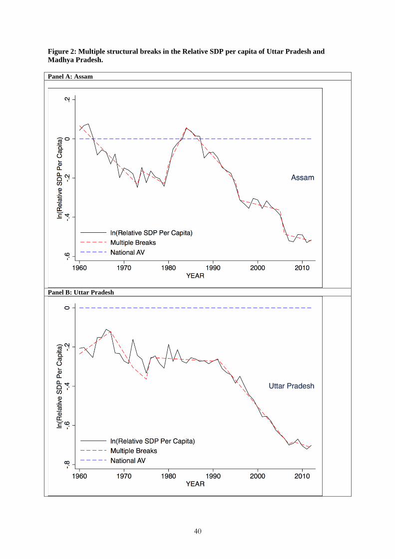
40

Figure 2: Multiple structural breaks in the Relative SDP per capita of Uttar Pradesh and

Madhya Pradesh.

Panel A: Assam

Panel B: Uttar Pradesh