30.August 2010

Parts of Chapters 5 & 7

Stratified and Piecewise Cox Ph Models

Example 1: Recall the Kleinbaum crossinghazards figure:In this study that compares surgery to no surgery,we might expect to see hazard functions foreach group as follows:

h(t|E)

E=1 (no surgery)

E=1

hazards cross

0 1 2 3 4 5 6days

0.0

0.2

0.4

0.6

0.8

E=0 (surgery)

Before 2 days, HR(1|0) < 1, whereas later,HR(1|0) > 1.The PH assumption is violated, since HR mustbe constant over the follow-up time.

1

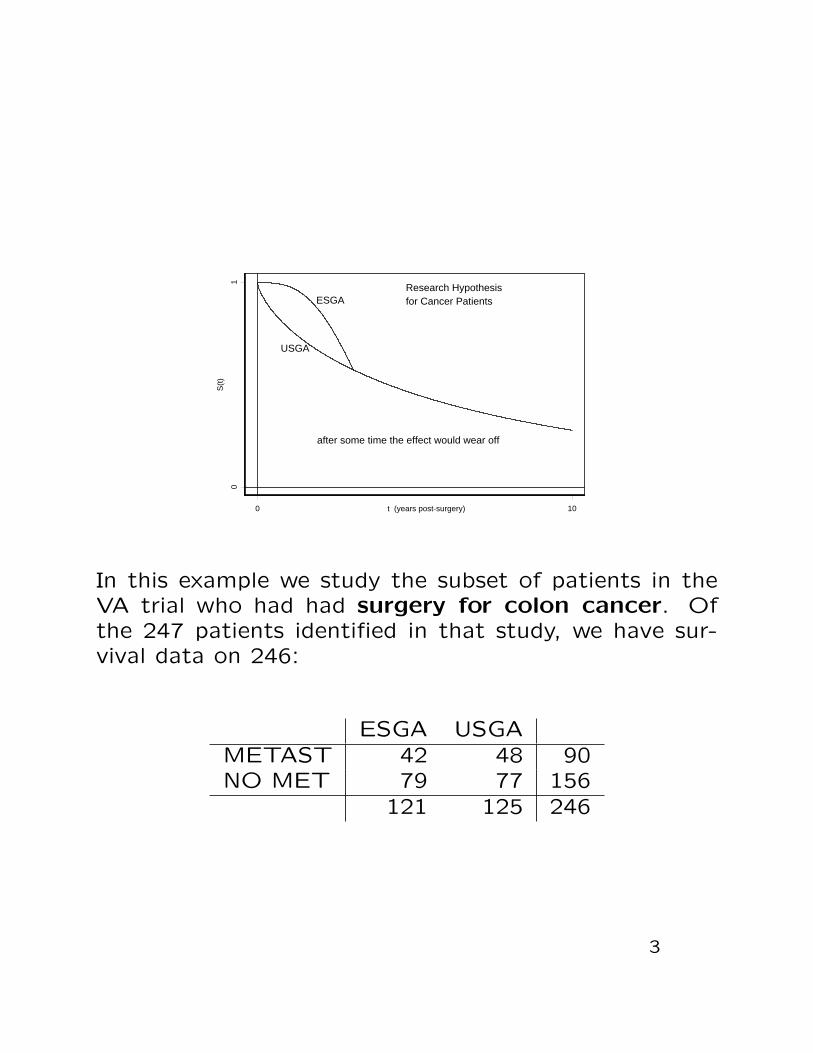
Example 2: Crossing survivor curves:VA Cooperative Trial No. 345This was a prospective randomized study conducted be-tween March 1992 and August 1994. Patients wererandomly assigned to either unsupplemented generalanesthesia and postoperative analgesia (USGA) or epidu-ral plus light general anesthesia and postoperative epidu-ral morphine (ESGA). procedures.

A researcher began a retrospective look ca. June 2003

• It is well established that the epidural protects cer-tain aspects of the immune function, and to blockthe stress response to surgical trauma.

• The epidural protocol has been common practice.

• Therefore, it was hypothesized that cancer surgerypatients should benefit from ESGA. The researchhypothesis is depicted in the following graph:

2

0 10t (years post-surgery)

01

S(t

)

Research Hypothesis for Cancer PatientsESGA

USGA

after some time the effect would wear off

In this example we study the subset of patients in theVA trial who had had surgery for colon cancer. Ofthe 247 patients identified in that study, we have sur-vival data on 246:

ESGA USGAMETAST 42 48 90NO MET 79 77 156

121 125 246

3

What time reveals for the No MET group:

0 1 2 3 4 5 6 7 8 9 10

Time (years post-surgery)

0.0

0.1

0.2

0.3

0.4

0.5

0.6

0.7

0.8

0.9

1.0

Pro

babi

lity

of S

urvi

val

No Metastasis Group

ESGAUSGA

p-value = 0.0448

Return to the 3.5-year mark:

0.0 0.5 1.0 1.5 2.0 2.5 3.0

Time (years post-surgery)

0.0

0.1

0.2

0.3

0.4

0.5

0.6

0.7

0.8

0.9

1.0

Pro

babi

lity

of S

urvi

val

ESGAUSGA

1.28-year 2.2-year

p-value = 0.761

.0822-year

3.5 years follow-up

4

The Cox PH structure imposes restrictions on thebehavior of survivor curves.

• With just one exposure variable x = 0,1, the rela-tionship is

h(t|1) = h(t|0) · exp(β).

• Let TRT = 0 if ESGA, 1 if USGA. Then

S(t|1) = (S(t|0))exp(β).

Cannot possibly model the crossing curves.

• Consider the results from the Cox PH fit to No MetData only

> coxph(Surv(TIME,CENSOR)~TRTcoef exp(coef) se(coef) z p

TRT -0.42 0.657 0.211 -1.99 0.046Likelihood ratio test=4.03 on 1 df, p=0.0447 n=156

5

0 1 2 3 4 5 6 7 8

Time (years post-surgery)

0.0

0.1

0.2

0.3

0.4

0.5

0.6

0.7

0.8

0.9

1.0

Pro

babili

ty o

f S

urv

ival

No Met GroupCox PH model with TRT

USGAESGA

Time

Beta

(t)

for

TR

T

0.19 1.4 2.3 3.8 4.5 5.6 6.9 8.2

-2-1

01

2

Scaled Schoenfeld residual plot, and the Grambsch-Therneau(1994) test for PH assumption. The residual plot clearlydisplays that TRT varies with time.

> PH.testrho chisq p

TRT -0.174 2.86 0.0906

6

Example 3: Divergent survivor curvesAustralian study of heroin addicts, Caplehorn, etal. (1991)

• two methadone treatment clinics

• T = days remaining in treatment( = days until drop out of clinic)

• clinics differ in overall treatment policies

• 238 patients in the study

Description of ADDICTS data set

Data set: ADDICTSColumn 1: Subject IDColumn 2: Clinic (1 or 2) ← exposure variableColumn 3: Survival status

0 = censored1 = departed clinic

Column 4: Survival time in daysColumn 5: Prison record ← covariate

0 = none, 1 = anyColumn 6: Maximum methadone dose (mg/day)← covariate

7

Part I: The following is R code, along with modifiedoutput, that fits two K-M curves not adjusted forany covariates to the survival data.

> addict.fit <- survfit(Surv(Days.survival,Status)~Clinic,data = ADDICTS)

> addict.fitn events mean se(mean) median 0.95LCL 0.95UCL

Clinic=1 163 122 432 22.4 428 348 514Clinic=2 75 28 732 50.5 NA 661 NA> survdiff(Surv(Days.survival,Status)~Clinic,data = ADDICTS)

N Observed Expected (O-E)^2/E (O-E)^2/VClinic=1 163 122 90.9 10.6 27.9Clinic=2 75 28 59.1 16.4 27.9Chisq= 27.9 on 1 degrees of freedom, p= 1.28e-007> plot(addict.fit, lwd = 3,col = 1,type = "l",lty=c(1, 3),

cex=2,lab=c(10,10,7),...)

Retention time (days) in methadone treatment

Pe

rce

nt

Re

tain

ed

0 100 200 300 400 500 600 700 800 900 1000 1100

01

02

03

04

05

06

07

08

09

01

00

Retention of Heroin Addicts in Methadone Treatment Clinics

Clinic 2

Clinic 1

Figure 1. K-M curves for ADDICTS not adjusted forcovariates.

8

Results:

• The log-rank test is highly significant with p -value=1.28× 10−7.

• The graph in Figure 1 glaringly confirms this differ-ence.

• This graph shows curve for clinic 2 is always abovecurve for clinic 1.

• Curves diverge, with clinic 2 being dramatically bet-ter after about one year in retention of patients inits treatment program.

• Lastly, this suggests the PH assumption is not sat-isfied.

9

Part II: The Cox PH model We now fit a Cox PHmodel which adjusts for the three predictor variables.This hazard model is

h(t|x) = h0 exp(β1Clinic + β2Prison + β3Dose).

A summary of the R output is:

> fit1 <- coxph(Surv(Days.survival,Status) ~ Clinic+Prison+Dose,data = ADDICTS,x = T) # Fits a Cox PH model

> fit1coef exp(coef) se(coef) z p

Clinic -1.0098 0.364 0.21488 -4.70 2.6e-006Prison 0.3265 1.386 0.16722 1.95 5.1e-002Dose -0.0354 0.965 0.00638 -5.54 2.9e-008

Likelihood ratio test=64.6 on 3 df, p=6.23e-014 n= 238> testph <- cox.zph(fit1) # Tests the proportional

# hazards assumption> print(testph) # Prints the results

rho chisq pClinic -0.2578 11.19 0.000824Prison -0.0382 0.22 0.639324Dose 0.0724 0.70 0.402755GLOBAL NA 12.62 0.005546> par(mfrow = c(2, 2))> plot(testph) # Plots the scaled Schoenfeld residuals.

10

Time

Beta

(t)

for

Clin

ic

45 150 220 340 470 580 740 850

-4-2

02

4

Time

Beta

(t)

for

Prison

45 150 220 340 470 580 740 850-3

-2-1

01

23

Time

Beta

(t)

for

Dose

45 150 220 340 470 580 740 850

-0.2

0.0

0.1

0.2

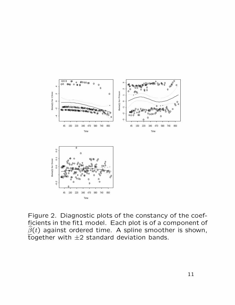
Figure 2. Diagnostic plots of the constancy of the coef-ficients in the fit1 model. Each plot is of a component ofβ(t) against ordered time. A spline smoother is shown,together with ±2 standard deviation bands.

11

Results:

• The GLOBAL test (a LRT) for non-PH is highly sta-tistically significant with p -value = 0.005546.

• The p -values for Prison and Dose are very large,supporting that these variables are time-independent.

• The Grambsch-Therneau test has a p -value = 0.000824for Clinic. This provides strong evidence that thevariable Clinic violates the PH assumption and con-firms what the graph in Figure 1 suggests.

• The plot of β1(t), the coefficient for Clinic, againstordered time in Figure 2 provides further supportingevidence of this violation.

• We recommend finding a function g(t) to multiplyClinic by; that is, create a defined time-dependentvariable, and then fit an extended Cox model.

12

Since the Cox PH model is inappropriate, the followingstrategies are employed:

• analyze by stratifying on the exposure variable;that is, do not fit any regression model, and, in-stead obtain the Kaplan-Meier curve for each groupseparately;

• to adjust for other significant factor effects, useCox model stratified on exposure variable E.

> coxph(Surv(time,status)~ X1+X2+· · ·+strata(E))

• fit a Cox PH model that includes a time-dependentvariable which measures the interaction of exposurewith time. This model is called an extended Coxmodel. We try to find the point in time t0 wherethe hazard rates change. Then fit a piecewise CoxPh model over these two time intervals.

13

Part III: Stratified Cox model

Suppose we have j = 1,2, . . . , s, i.e., s strata. For eachstratum we assume the Cox PH model:

hj(t|x) = h0j(t) exp(x′β), j = 1, . . . , s.

The regression coefficients are assumed to be the samein each stratum although the baseline hazard functionsmay ne different and completely unrelated. Then usingonly the data for those subjects in the jth stratum,we have:

Let t(1j), . . . , t(rj) denote the r ≤ nj ordered (uncensored)death times, so that t(kj) is the kth ordered death time.Let x(kj) denote the vector of covariates associated withthe individual who dies at t(kj).

Cox’s partial likelihood function for the jth stratum:

Lcj(β) =r∏

kj=1

exp(x′(kj)β)∑

l∈R(t(kj))exp(x′lβ)

.

Then estimation and testing methods are as before,where the partial log likelihood to be maximized is givenby

LLc(β) =s∑

j=1

LLcj(β).

14

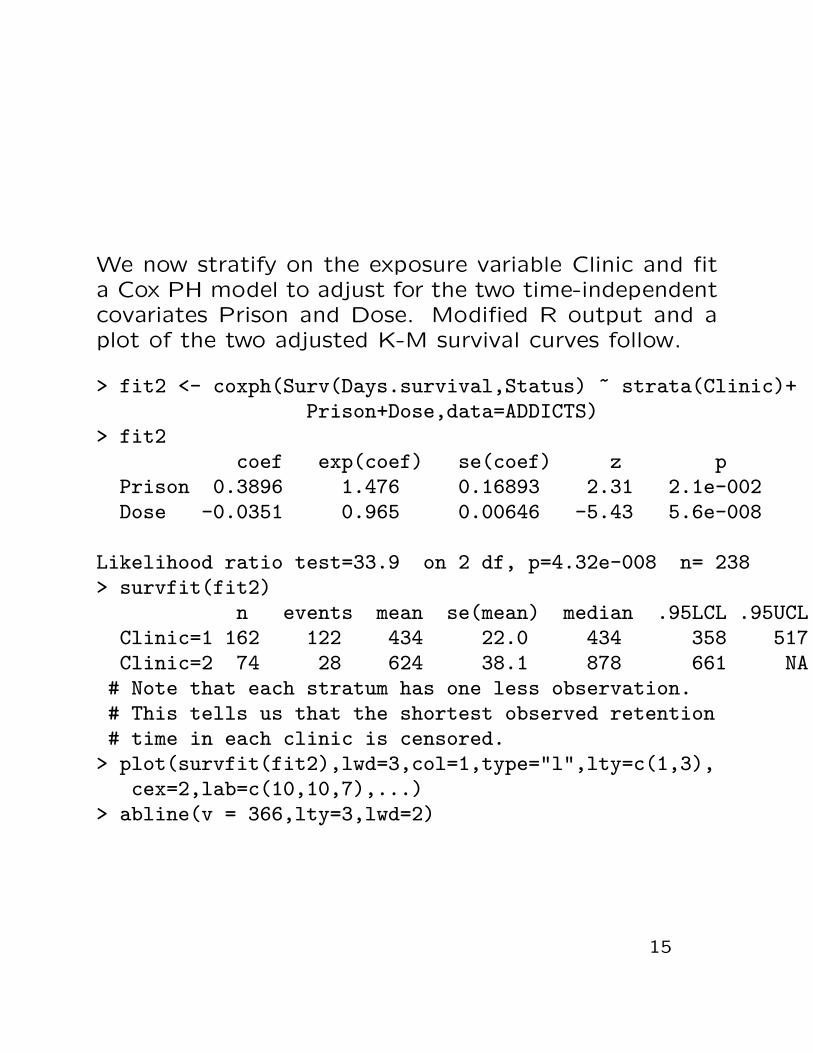
We now stratify on the exposure variable Clinic and fita Cox PH model to adjust for the two time-independentcovariates Prison and Dose. Modified R output and aplot of the two adjusted K-M survival curves follow.

> fit2 <- coxph(Surv(Days.survival,Status) ~ strata(Clinic)+Prison+Dose,data=ADDICTS)

> fit2coef exp(coef) se(coef) z p

Prison 0.3896 1.476 0.16893 2.31 2.1e-002Dose -0.0351 0.965 0.00646 -5.43 5.6e-008

Likelihood ratio test=33.9 on 2 df, p=4.32e-008 n= 238> survfit(fit2)

n events mean se(mean) median .95LCL .95UCLClinic=1 162 122 434 22.0 434 358 517Clinic=2 74 28 624 38.1 878 661 NA

# Note that each stratum has one less observation.# This tells us that the shortest observed retention# time in each clinic is censored.> plot(survfit(fit2),lwd=3,col=1,type="l",lty=c(1,3),

cex=2,lab=c(10,10,7),...)> abline(v = 366,lty=3,lwd=2)

15

Retention time (days) in methadone treatment

Pe

rce

nt

Re

tain

ed

0 100 200 300 400 500 600 700 800 900

01

02

03

04

05

06

07

08

09

01

00

Adjusted Survival CurvesStratified by Clinic

Clinic 2

Clinic 1

1 year

Figure 3. K-M curves adjusted for covariates Prison andDose, stratified by Clinic.

Results:

• Figure 3 provides same pictorial evidence as Fig-ure 1; that is, curve for clinic 2 is always above clinic1’s curve, with clinic 2 being dramatically better inretention of patients in its treatment program afterabout one year.

• The estimated coefficients for Prison and Dose donot change much. This gives good evidence thatthe stratified model does satisfy the PH assumtion;hence, this analysis is valid.

• Figure 3 provides a picture of the effect of Clinic onretention of patients. But by stratifying on Clinic,we get no estimate of its effect; i.e., no estimated

16

β1 coefficient. Hence, we cannot obtain a hazardratio for Clinic.

• The exposure variable Clinic must be in the modelin order to obtain a hazard for it. For this reason,we look now to the extended Cox model.

Part IV: A Piecewise Cox PH model analysis

Here we use a model that contains two heavyside func-tions, g1(t) and g2(t), with t0, the change point, to bedetermined. The hazard model is

h(t|x(t)) = h0(t) exp (β1Prison + β2Dose + γ1(Clinic× g1(t))+ γ2(Clinic× g2(t)))

where

g1(t) =

{1 if t < t00 if t ≥ t0

g2(t) =

{1 if t ≥ t00 if t < t0

and

Clinic =

{1 if Clinic=10 if Clinic=2.

(1)

The hazard ratio for the exposure variable Clinic nowvaries with time. It assumes two distinct values de-pending whether time < t0 days or time ≥ t0 days. Theform of the HR is

t < t0 : HR = exp(γ1)t ≥ t0 : HR = exp(γ2) .

Time-dependent covariates effect the rate for upcomingevents. In order to implement an extended Cox modelproperly in R using the coxph function, one must usethe Anderson-Gill (1982) formulation of the proportionalhazards model as a counting process. They treat

17

each subject as a very slow Poisson process. A censoredsubject is not viewed as incomplete, but as one whoseevent count is still zero. For a brief introduction to thecounting process approach, see Appendix 2 of Hosmer& Lemeshow (1999) and the online manual S-PLUS2000, Guide to Statistics, Vol 2, Chapter 10. Klein &Moeschberger (1997, pages 70−79) discuss this count-ing process formulation. They devote their Chapter 9 tothe topic of modelling time-dependent covariates. Fora more advanced and thorough treatment of countingprocesses in survival analysis, see Fleming and Harring-ton (1991).

The ADDICTS data set must be reformulated to matchthe Anderson-Gill notation. To illustrate this, considerthe following cases: In both cases the t denotes the pa-tient’s recorded survival time, whether censored or not.

Case 1: For t < t0, g1(t) = 1 and g2(t) = 0. Here apatient’s data record is just one row and looks like this:

Start Stop Status Dose Prison Clinicg1t Clinicg2t0 t same same same Clinic 0

Case 2: For t ≥ t0, g1(t) = 0 and g2(t) = 1. Here apatient’s data record is formulated into two rows andlooks like this:

18

Start Stop Status Dose Prison Clinicg1t Clinicg2t0 t0 0 same same Clinic 0t0 t same same same 0 Clinic

The following R program puts the ADDICTS data setinto the counting process form, finds the optimal changepoint t0; i.e., the time which maximizes the profile logpartial likelihood. We then fit the model and reportresults.

> ADDICTS<-read.table("C://ADDICTS.txt",header=T)> ADDICTS$Clinic[ADDICTS$Clinic==2]<-0> names(ADDICTS)[1] "ID" "Clinic" "Status" "Days.survival"[5] "Prison" "Dose"> attach(ADDICTS)> library(survival)> optimal.change.point(ADDICTS,Days.survival,Status,Clinic)

changepoint loglik119 461 -683.2117> #Thus, in the survSplit function, let cut = 461.> #Use the function extcox.1Et to obtain the dataset in the> #Andersen-Gill counting process format> AG<-extcox.1Et(ADDICTS,Days.survival,Status,Clinic,461)> names(AG)[1] "ID" "Clinic" "Status" "Days.survival"[5] "Prison" "Dose" "end" "status"[9] "trt" "start" "ET1" "ET2"> fit4<-coxph(Surv(start,end,status)~Prison+Dose+ET1+ET2,

data=AG)

19

> fit4Call: coxph(formula = Surv(start, end, status) ~ Prison +

Dose + ET1 + ET2, data = AG)

coef exp(coef) se(coef) z pPrison 0.3890 1.476 0.16859 2.31 2.1e-02Dose -0.0354 0.965 0.00645 -5.48 4.3e-08ET1 0.4887 1.630 0.23396 2.09 3.7e-02ET2 2.3971 10.991 0.52998 4.52 6.1e-06

Likelihood ratio test=79 on 4 df, p=3.33e-16 n= 337> temp<-cox.zph(fit4)> temp

rho chisq pPrison -0.0176 0.0465 0.829Dose 0.0829 0.9305 0.335ET1 0.0264 0.1059 0.745ET2 -0.0089 0.0117 0.914GLOBAL NA 1.0595 0.901> windows()> par(mfrow=c(2,2))> plot(temp)

20

This graph is automatically outputted from the

optimal.change.point function.

0 200 400 600 800 1000

−69

0−

689

−68

8−

687

−68

6−

685

−68

4−

683

change point (distinct survival times)

log−

likel

ihoo

d

Profile of the log−partial likelihood for a piecewise Cox PH model

21

Time

Bet

a(t)

for

Pris

on

45 220 470 740

−3

−1

13

Time

Bet

a(t)

for

Dos

e45 220 470 740

−0.

20.

00.

2

Time

Bet

a(t)

for

ET

1

45 220 470 740

−6

−2

02

Time

Bet

a(t)

for

ET

2

45 220 470 740

−30

−10

10

95% C.I.’s for the Clinic’s HR’st < 461: [1.03,2.58]

t ≥ 461: [3.89,31.06]

22

Results:

• The output shows a significant HR = 1.63 with p -value = 0.037 for the effect of Clinic when time< 461 days. For t ≥ 461, the HR = 10.99 is highlysignificant with p -value = 6.1× 10−6.

• The table reports confidence intervals for the twoHR’s. The general form of these 95% C.I.’s isexp(coef ± 1.96 × se(coef)). The 95% C.I. for theHR when t precedes 461 is a bit above 1 and isnarrow. This supports a significant effect due toclinic during the first year and has good precision.The 95% C.I. for the HR when t ≥ 461 lies above1 and is very wide showing a lack of precision.

• These findings support what was displayed in Fig-ure 3. But now it is quantified. There is strongstatistical evidence of a large difference in clinic sur-vival times after 461 days in contrast to a small andbut still significant difference in clinic survival timesprior to 461 days, with clinic 2 always doing bet-ter in retention of patients than clinic 1. After 461days, clinic 2 is nearly 11 times more likely to re-tain a patient longer than clinic 1. Also, clinic 2 has111≈ 10% the risk of clinic 1 of a patient leaving its

methadone treatment program.

23

• See Kleinbaum (1996, Chapter 6) for further anal-ysis of this data.

• An alternative regression quantile analysis as pre-sented in Chapter 8 may be appropriate when thePH assumption