exascale deep learning for climate analytics - arxiv.org · exascale deep learning for climate...
TRANSCRIPT
Exascale Deep Learning for Climate AnalyticsThorsten Kurth∗
Nathan Luehr†[email protected]
Jack Deslippe∗[email protected]
Sean Treichler†[email protected]
Everett Phillips†[email protected]
Massimiliano Fatica†[email protected]
Joshua Romero†[email protected]
Ankur Mahesh∗[email protected]
Prabhat∗[email protected]
Mayur Mudigonda∗[email protected]
Michael Matheson‡[email protected]
Michael Houston†[email protected]
Abstract—We extract pixel-level masks of extreme weatherpatterns using variants of Tiramisu and DeepLabv3+ neural net-works. We describe improvements to the software frameworks,input pipeline, and the network training algorithms necessaryto efficiently scale deep learning on the Piz Daint and Summitsystems. The Tiramisu network scales to 5300 P100 GPUs witha sustained throughput of 21.0 PF/s and parallel efficiency of79.0%. DeepLabv3+ scales up to 27360 V100 GPUs with a sus-tained throughput of 325.8 PF/s and a parallel efficiency of 90.7%in single precision. By taking advantage of the FP16 Tensor Cores,a half-precision version of the DeepLabv3+ network achieves apeak and sustained throughput of 1.13 EF/s and 999.0 PF/srespectively.
I. JUSTIFICATIONWe apply segmentation architectures to climate datasets;
achieving state-of-the-art weather pattern masks. We scalethe architectures to 27360 Volta GPUs, obtaining a peak(sustained) FP16 performance of 1.13 EF/s (1.0 EF/s). Wedeveloped methodologies at system level and several deeplearning algorithmic innovations to achieve this unprecedentedscaling.
II. PERFORMANCE ATTRIBUTES
Performance Attribute Our submissionCategory of Achievement Peak performance, Time-to-
solutionType of Method Used Deep LearningResults reported on basis of Whole application
including I/OPrecision reported Mixed precisionSystem scale Measured on full systemMeasurement mechanism Application timers
III. OVERVIEW
A. Pattern Detection for Characterizing Extreme Weather
Climate change poses a major challenge to humanity inthe 21st century. Several nations are considering adaptationand mitigation strategies pertaining to global, mean quantitiessuch as temperature, or sea-level rise. Increasingly, state andlocal governments are interested in the question of howextreme weather events will change and affect their local
∗ Lawrence Berkeley National Laboratory, Berkeley, CA 94720, USA† NVIDIA, Santa Clara, CA 95051, USA‡ Oak Ridge National Laboratory, Oak Ridge, TN 37831, USA
communities. For instance, the state of California receivesover 50% of its rainfall through Atmospheric Rivers (ARs),and Water Resource Management planners are interested inunderstanding if AR tracks will shift in the future, potentiallyresulting in a dramatic shortfall in fresh water supply. In thestate of Florida, homeowners are interested in understandingif Tropical Cyclones (TCs) or hurricanes will become moreintense and start making landfall more often. This has a directimpact on home prices and the insurance industry. TCs havecaused the US economy over $200B worth of damage in 2017,and a range of stakeholders are interested in a more carefulcharacterization of the change in number and intensity of suchextreme weather patterns in the coming decades.
In order to address these important questions, climate sci-entists routinely configure and run high-fidelity simulationsunder a range of different climate change scenarios. Eachsimulation produces 10s of TBs of high-fidelity output whichrequires automated analysis. Thus far, climate data analystshave relied entirely upon multi-variate threshold conditions forprescribing extreme weather patterns [1]. Recent efforts [2],[3], [4] have shown that deep learning can be successfullyapplied for detection, classification and localization of extremeweather patterns. In this paper, we push the frontier of deeplearning methods to extract high-quality, pixel-level segmen-tation masks of weather patterns.
In this work, we use the TensorFlow [5], [6] deep learningframework, which allows the programmatic definition of evenvery complicated network graphs in tens of lines of Pythoncode. TensorFlow provides portability with its capability tomap a graph onto multi- and many-core CPUs as well asGPUs. Due to the heavy use of linear algebra-based primitives(e.g. convolutions), most networks (including ours) performvery well on GPUs. The graph also captures the parallelismavailable in the computation, and TensorFlow uses a dynamicscheduler to select which operation (or layer) to computebased on the availability of inputs. (Scheduling is performedindependently on each process in a distributed job, leadingto challenges with collective communication described inSection V-A3.)
A deep learning model is trained by comparing its output toknown labels, using a loss function to quantify the differencesbetween the two. The model parameters (e.g. convolution
SC18, November 11-16, 2018, Dallas, Texas, USA978-1-5386-8384-2/18/$31.00 c©2018 IEEE
arX
iv:1
810.
0199
3v1
[cs
.DC
] 3
Oct
201
8
decoder
ASPP
encoder7×7 conv, 64, /2
1152×768, 16
input
3×3 maxpool, /2
1×1 conv, 64
3×3 conv, 64
1×1 conv, 256
288×192, 64
3×
1×1 conv, 128
3×3 conv, 128
1×1 conv, 512
144×96, 256
4×
1×1 conv, 256
3×3 conv, 256, d 2
1×1 conv, 1024
144×96, 512
6×
1×1 conv, 512
3×3 conv, 512, d 4
1×1 conv, 2048
144×96, 1024
3×
1×1 conv, 256
3×3 conv, 256, d 12
3×3 conv, 256, d 24
3×3 conv, 256, d 36
1×1 conv, 256
144×96, 1024
144×96, 2048
3×3 deconv, 256, /2
1×1 conv, 48
3×3 conv, 64
3×3 conv, 128
3×3 conv, 256
3×3 conv, 256
3×3 deconv, 256, /2
3×3 deconv, 256, /2
1×1 conv, 3
3×3 conv, 256
3×3 conv, 256
1152×768, 3
output
288×192, 256
1152×768, 2561152×768, 128
288×192, 256
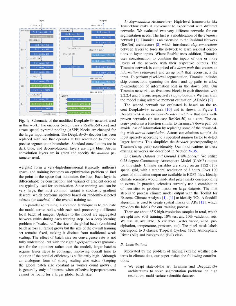
Fig. 1: Schematic of the modified DeepLabv3+ network usedin this work. The encoder (which uses a ResNet-50 core) andatrous spatial pyramid pooling (ASPP) blocks are changed forthe larger input resolution. The DeepLabv3+ decoder has beenreplaced with one that operates at full resolution to produceprecise segmentation boundaries. Standard convolutions are indark blue, and deconvolutional layers are light blue. Atrousconvolution layers are in green and specify the dilation pa-rameter used.
weights) form a very-high-dimensional (typically millions)space, and training becomes an optimization problem to findthe point in the space that minimizes the loss. Each layer isdifferentiable by construction, and variants of gradient descentare typically used for optimization. Since training sets can bevery large, the most common variant is stochastic gradientdescent, which performs updates based on randomly-selectedsubsets (or batches) of the overall training set.
To parallelize training, a common technique is to replicatethe model across ranks, with each rank processing a differentlocal batch of images. Updates to the model are aggregatedbetween ranks during each training step. As a deep learningproblem is “scaled out,” the size of the global batch (combinedbatch across all ranks) grows but the size of the overall trainingset remains fixed, making it distinct from traditional weakscaling. The effect of batch size on convergence rate is notfully understood, but with the right hyperparameters (parame-ters for the optimizer rather than the model), larger batchesrequire fewer steps to converge, improving overall time tosolution if the parallel efficiency is sufficiently high. Althoughan analogous form of strong scaling also exists (keepingthe global batch size constant as worker count grows), itis generally only of interest when effective hyperparameterscannot be found for a larger global batch size.
1) Segmentation Architecture: High-level frameworks likeTensorFlow make it convenient to experiment with differentnetworks. We evaluated two very different networks for oursegmentation needs. The first is a modification of the Tiramisunetwork [7]. Tiramisu is an extension to the Residual Network(ResNet) architecture [8] which introduced skip connectionsbetween layers to force the network to learn residual correc-tions to layer inputs. Where ResNet uses addition, Tiramisuuses concatenation to combine the inputs of one or morelayers of the network with their respective outputs. TheTiramisu network is comprised of a down path that creates aninformation bottle-neck and an up path that reconstructs theinput. To perform pixel-level segmentation, Tiramisu includesskip connections spanning the down and up paths to allowre-introduction of information lost in the down path. OurTiramisu network uses five dense blocks in each direction, with2,2,2,4 and 5 layers respectively (top to bottom). We then trainthe model using adaptive moment estimation (ADAM) [9].
The second network we evaluated is based on the re-cent DeepLabv3+ network [10] and is shown in Figure 1.DeepLabv3+ is an encoder-decoder architure that uses well-proven networks (in our case ResNet-50) as a core. The en-coder performs a function similar to Tiramisu’s down path butavoids loss of information by replacing some of the downscal-ing with atrous convolution. Atrous convolutions sample theinput sparsely according to a specified dilation factor to detectlarger features. This simplifies the decoder (corresponding toTiramisu’s up path) considerably. Our modifications to theseexisting networks are described in Section V-B5.
2) Climate Dataset and Ground Truth Labels: We utilize0.25-degree Community Atmosphere Model (CAM5) outputfor this study. Climate variables are stored on an 1152×768spatial grid, with a temporal resolution of 3 hours. Over 100years of simulation output are available in HDF5 files. Ideally,climate scientists would hand-label pixel masks correspondingto events. In practice, scientists currently use a combinationof heuristics to produce masks on large datasets. The firststep is to process climate model output with the Toolkit forExtreme Climate Analysis [1], [11] to identify TCs. A floodfillalgorithm is used to create spatial masks of ARs [12], whichprovides the labels for our training process.
There are about 63K high-resolution samples in total, whichare split into 80% training, 10% test and 10% validation sets.We use all available 16 variables (water vapor, wind, pre-cipitation, temperature, pressure, etc). The pixel mask labelscorrespond to 3 classes: Tropical Cyclone (TC), AtmosphericRiver (AR) and background (BG) class.
B. Contributions
Motivated by the problem of finding extreme weather pat-terns in climate data, our paper makes the following contribu-tions:
• We adapt state-of-the art Tiramisu and DeepLabv3+architectures to solve segmentation problems on highresolution, multi-variate scientific datasets.
• We make a number of system-level innovations in datastaging, efficient parallel I/O, and optimized networkingcollectives to enable our DL applications to scale tothe largest GPU-based HPC systems in the world (Sec-tion V-A).
• We make a number of algorithmic innovations to enableDL networks to converge at scale (Section V-B).
• We demonstrate good scaling on up to 27360 GPUs, ob-taining 999.0 PF/s sustained performance and a parallelefficiency of 90.7% (Section VII) for half precision. Thepeak performance we obtained at that concurrency andprecision was 1.13 EF/s.
• Our code is implemented in TensorFlow and Horovod;our performance optimizations are broadly applicable tothe general deep learning + HPC community, our stackis already being used by several other projects.
While our work is conducted in the context of a specificscience driver, most of our proposed innovations are applicableto generic deep learning workloads at scale.
IV. STATE OF THE ART
A. State-of-the-art in Scientific Deep Learning
In recent years, the scientific community has begun toadopt deep learning methods and frameworks as tools forscientific analysis and discovery [13], [14], [15], [16], [17],[18]. Early applications were focused on adapting off-the-shelfconvolutional neural networks from natural image processingapplications or recurrent neural networks from speech recog-nition applications (for a review see [19]). There is currentlya shift in the community towards incorporating scientificprinciples (e.g. physical laws such as energy or momentumconservation) and common assumptions (e.g. temporal and/orspatial coherence). Some recent examples in the domain areasrelated to ours include simulation of local wind field patternsvia coupled autoencoder architectures [20], turbulence model-ing for climate simulations via deep networks trained with lossfunctions that incorporate physical terms [21], and supervisedapplications of extreme weather pattern detection [2]. Thefield of physics-informed deep learning for scientific andengineering applications is in its infancy, and this paper isa timely contribution focused on exploring the computationallimits of representative architectures that many of the aboveapproaches are based on.
B. State-of-the-art in Large-Scale Deep Learning
Modern-day deep neural networks build upon the worklaid out by McCullogh and Pitt [22], and Rosenblatt (per-ceptron) [23]. While forming the foundation for deep learn-ing, these early models often struggled as the network sizeincreases, limiting their utility in the analysis of complexsystems. More recently, work by Krizhevsky [24] opened theflood gates for modern day Deep Learning, showing impres-sive performance on hard vision tasks using large superviseddeep networks. This breakthrough was made possible in partby the rapid increase in computational power of moderncomputing systems. Since then, the complexity of tasks and
the size of the networks have been growing steadily over theyears, arguably requiring larger and more powerful platforms.
There has been more recent work on scaling deep learningup to larger node counts and performance. Preferred Networks,Inc. demonstrated ResNet-50 converging to 75% accuracy in15 minutes using the ChainerMN [25] framework on 1024NVIDIA Tesla P100 GPUs at a total global batch size of 32Kfor 90 epochs [26]. Jia at al. [27], concurrent with this work,demonstrated scaling to 2048 NVIDIA Tesla P40 GPUs at64K batch size, achieving convergence in 6.6 minutes usingTensorFlow. To effectively utilize leadership class systems,we need to push scaling significantly further than previouswork. Most work on classification networks uses relativelysmall images from the computer vision community. Our workextends Deep Learning to handle much larger input in the formof snapshots from a scientific simulation. These "images" canbe millions of pixels in size and generally have many morechannels than the red, green, and blue of commodity imagingsensors. We are also contending with a significantly largerdataset that pushes the limits of the file system and requiresnew data handling techniques.
V. INNOVATIONS
A. System Innovations
1) High speed parallel data staging: Modern neural net-works require large amounts of input data and thereforetraining can easily be bottlenecked by an inability to bringinput data to the GPU in a timely fashion. For instance,a single GPU training our modified Tiramisu network canconsume 189 MB/s, already above the capabilities of a localhard drive, which means the 6 GPUs on a Summit noderequire a combined 1.14 GB/s. A training run using 1024nodes therefore requires a sustained read bandwidth of 1.16TB/s, and running on the full Summit system will require 5.23TB/s, more than twice the target performance of the GPFS filesystem.
Summit makes available 800 GB of high-speed SSD storageon each node to help with local bandwidth needs. While atraining data set can be quite large (the climate data used inthis study is currently 3.5 TB), in a distributed training setting,it suffices for each node to have access to a significant fractionof the overall data set. The images selected by each rank arecombined to form a batch, so a sufficient (and independentlyselected) set of samples for each rank to choose from resultsin batches that are statistically very similar to a batch selectedfrom the entire data set. In our experiments, 250 images perGPU (1500 per node) are sufficient to maintain convergence.
Unfortunately, a naive staging script that asked each of 1024nodes to copy its own subset of the full data set from GPFSrequired 10-20 minutes to complete and rendered the globalfile system nearly unusable for other users of the machineduring that time. With this approach, each individual file fromthe data set was being read by 23 nodes on average. To addressthis, we developed a distributed data staging system that firstdivides the data set into disjoint pieces to be read by eachrank. Each rank’s I/O throughput was further improved by
running multiple threads that perform file reads in parallel– using eight threads instead of one increased the achievedread bandwidth from 1.79 GB/s on average to 11.98 GB/s,an improvement of 6.7×. Once all files in the data set havebeen read from GPFS, point-to-point MPI messages are usedto distribute copies of each file to other nodes that requireit. This approach takes advantage of the significantly higherbandwidth of the Infiniband network and places no further loadon the file system. Our improved script is able to stage in datafor 1024 (4500) nodes on Summit in under 3 (7) minutes.
On Piz Daint, where no local SSDs are available, the onlynode local storage with sufficient bandwidth to feed the P100GPU is the Linux tmpfs (DRAM), which has much morelimited capacity.
2) Optimized data ingestion pipeline: Although the stagingof input data into fast local storage eliminates bottlenecks andvariability from global file system reads, optimization is alsorequired for the TensorFlow input pipeline that reads the inputfiles and converts them into the tensors that are fed throughthe network. By default, the operations to read and transforminput data are placed in the same operation graph as thenetworks themselves, causing idle time on the GPU while theCPU performs input-related tasks. This serialization can beeliminated by enabling the prefetching option of TensorFlowdatasets, which allows the input pipeline to run ahead of restof the network, placing processed input data into a queue.As long as the queue remains non-empty, the network canobtain its next input immediately upon completion of theprevious one. The queue depth can be made deep enough toinsulate against variability in the input processing rate, butthe average production rate must still exceed the average con-sumption rate. As a further optimization, TensorFlow allowsfor concurrent processing of multiple input files using its mapoperator; however, the HDF5 library used to read the climatedata serializes all operations, negating the benefit of paralleloperation. By using the Python multiprocessing module,we were able to transform these parallel worker threads intoparallel worker processes, each using its own instance of theHDF5 library. With 4 background processes taking care ofreading and processing input data, the input pipeline can moreclosely match the training throughput of both networks, evenwhen using FP16 precision.
3) Hierarchical all-reduce: Network training is distributedacross multiple GPUs using Horovod [28]. Horovod is aPython module that uses MPI to transform a single-processTensorFlow application into a data-parallel implementation.Each MPI rank creates its own identical copy of the Tensor-Flow operation graph. Horovod then inserts all-reduce oper-ations into the back-propagation computation to average thecomputed gradients from each rank’s network. Ranks updatetheir local models independently, but (assuming consistentinitialization) the use of gradients averaged across all theranks results in identical updates (i.e. synchronous distributedtraining). Although it is possible for a TensorFlow+Horovodimplementation to use multiple GPUs per rank, we adoptedthe simpler approach of using a different MPI rank for each
GPU (i.e. 6 ranks per node on Summit), allowing the samecode to be used on both Summit and Piz Daint. Horovod hasbeen shown to have good scalability up to 1024 GPUs, but aswe scaled further, we saw a dramatic loss in parallel efficiencyresulting from two issues.
The first issue was a bottleneck on the first rank, which actsas a centralized scheduler for Horovod operations. As eachTensorFlow process is independently scheduling the operationsin its graph, different ranks might attempt to execute their all-reduce operations in different orders, resulting in deadlock.Horovod resolves this by dynamically reordering all-reduceoperations to be consistent across all ranks. Each rank sendsa message to the controller (rank 0) indicating readiness toperform a given all-reduce operation. Once the controller hasreceived messages from all ranks for one or more operations,it sends a return message to every rank with an ordered listof tensors on which to perform collective operations. Ournetwork has over a hundred allreduce operations per step,forcing the controller to receive and then send millions ofmessages per second for larger jobs. A distribution of thescheduling load is not possible, as all ranks must agree on atotal order of collective operations to perform, so we choseinstead to perform hierarchical aggregation of the controlmessages. The ranks are organized into a tree of configurableradix r, and each node in the tree waits for readiness messagesfrom all of its direct children (and its own local operation)before sending a readiness message to its parent in the tree.Rank 0 sits at the root of the tree and uses the original Horovodalgorithm for scheduling, but operates as if there were onlyr+1 ranks to coordinate. When a rank receives a messageto start collective operations, it first relays that message to itschildren (if any) and then initiates the collective. This recursivebroadcast approach guarantees that no rank sends or receivesmore than r+1 messages for each tensor, reducing the messageload to mere thousands of messages per second, regardless ofscale. Tuning of broadcast tree shapes can be important whenlatency is a concern, but TensorFlow’s dynamic schedulermakes it fairly tolerant to small latency differences, and weobserved no measureable performance difference for values ofr between 2 and 8.
The second issue to address was the performance of the col-lective all-reduce operations themselves. The existing Horovodimplementation is able to reduce data residing on GPUs intwo different ways, either by a standard MPI_Allreduceor by using the NVIDIA Collective Communications Library(NCCL)[29]. Both have their strengths: MPI often uses tree-based communication patterns for performance at scale, whileNCCL uses a systolic ring approach that takes advantage of thebandwidth of GPUs that are connected with NVLink within aSummit node. To obtain both the scalability of MPI and thelocal bandwidth improvements of NCCL, we implemented ahybrid all-reduce approach. Data is first reduced across theGPUs within a node using NCCL. Once those 6 ranks have thesame locally-reduced data, 4 of the ranks (two on each CPUsocket) each perform an MPI_Allreduce on a quarter of thedata, sharing with the corresponding rank on every other node
and obtaining their quarter of the final result. Finally, NCCLbroadcast operations are used within the node to ensure eachof the 6 GPUs has a full copy of the entire all-reduce result.The decision to have 4 local ranks perform MPI operationswas based on experimentation, but suggests that a 1:1 mappingbetween communicating processes and virtual network devicesis the most efficient strategy on Summit (each node has a dual-rail Mellanox IB ConnectX-5 EX adapter that is virtualized as4 IB devices). With only a single GPU per node, Piz Daintdoes not benefit from this hybrid all-reduce implementation,but with the trend towards higher GPU counts per node, weexpect this optimization to be beneficial on future machinesas well.
B. Deep Learning Innovations
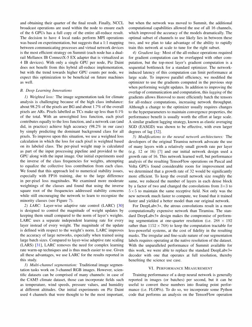
1) Weighted loss: The image segmentation task for climateanalysis is challenging because of the high class imbalance:about 98.2% of the pixels are BG and about 1.7% of the overallpixels are ARs. Pixels labelled as TCs make up less than 0.1%of the total. With an unweighted loss function, each pixelcontributes equally to the loss function, and a network can (anddid, in practice) achieve high accuracy (98.2% in our case)by simply predicting the dominant background class for allpixels. To improve upon this situation, we use a weighted losscalculation in which the loss for each pixel is weighted basedon its labeled class. The per-pixel weight map is calculatedas part of the input processing pipeline and provided to theGPU along with the input image. Our initial experiments usedthe inverse of the class frequencies for weights, attemptingto equalize the collective loss contribution from each class.We found that this approach led to numerical stability issues,especially with FP16 training, due to the large differencein per-pixel loss magnitudes. We examined more moderateweightings of the classes and found that using the inversesquare root of the frequencies addressed stability concernswhile still encouraging the network to learn to recognize theminority classes (see Figure 7).
2) LARC: Layer-wise adaptive rate control (LARC) [30]is designed to control the magnitude of weight updates bykeeping them small compared to the norm of layer’s weights.LARC uses a separate independent learning rate for everylayer instead of every weight. The magnitude of the updateis defined with respect to the weight’s norm. LARC improvesthe accuracy of large networks, especially when trained usinglarge batch sizes. Compared to layer-wise adaptive rate scaling(LARS) [31], LARC removes the need for complex learningrate warm-up techniques and is thus much easier to use. Givenall these advantages, we use LARC for the results reported inthis study.
3) Multi-channel segmentation: Traditional image segmen-tation tasks work on 3-channel RGB images. However, scien-tific datasets can be comprised of many channels: in case ofthe CAM5 climate dataset, those can incorporate fields suchas temperature, wind speeds, pressure values, and humidityat different altitudes. Our initial experiments on Piz Daintused 4 channels that were thought to be the most important,
but when the network was moved to Summit, the additionalcomputational capabilities allowed the use of all 16 channels,which improved the accuracy of the models dramatically. Theoptimal subset of channels to use likely lies in between thesetwo, and we plan to take advantage of the ability to rapidlytrain this network at scale to tune for the right subset.
4) Gradient lag: Most of the all-reduce operations requiredfor gradient computation can be overlapped with other com-putation, but the top-most layer’s gradient computation is asequential bottleneck for a standard optimizer. The network-induced latency of this computation can limit performance atlarge scale. To improve parallel efficiency, we modified theoptimizer to use the gradients computed in the previous stepwhen performing weight updates. In addition to improving theoverlap of communication and computation, this lagging of thegradients allows Horovod to more efficiently batch the tensorsfor all-reduce computations, increasing network throughput.Although a change to the optimizer usually requires changesto the hyperparameters to maintain convergence properties, theperformance benefit is usually worth the effort at large scale.A similar gradient lagging strategy, known as elastic averagingSGD (EASGD) was shown to be effective, with even largerdegrees of lag [32].
5) Modifications to the neural network architectures: Thedevelopers of the original Tiramisu network advocate the useof many layers with a relatively small growth rate per layer(e.g. 12 or 16) [7] and our initial network design used agrowth rate of 16. This network learned well, but performanceanalysis of the resulting TensorFlow operations on Pascal andVolta GPUs found considerable room for improvement andwe determined that a growth rate of 32 would be significantlymore efficient. To keep the overall network size roughly thesame, we reduced the number of layers in each dense blockby a factor of two and changed the convolutions from 3×3 to5×5 to maintain the same receptive field. Not only was thenew network much faster to compute, we found that it trainedfaster and yielded a better model than our original network.
For DeepLabv3+, the atrous convolutions result in a morecomputationally expensive network than Tiramisu. The stan-dard DeepLabv3+ design makes the compromise of perform-ing segmentation at one-quarter resolution (i.e. 288 × 192rather than 1152× 768) to keep the computation tractable forless-powerful systems, at the cost of fidelity in the resultingmasks. The irregular and fine-scale nature of our segmentationlabels requires operating at the native resolution of the dataset.With the unparalleled performance of Summit available forthis work, we were able to replace the standard DeepLabv3+decoder with one that operates at full resolution, therebybenefiting the science use case.
VI. PERFORMANCE MEASUREMENT
Training performance of a deep neural network is generallyreported in images (or batches) per second, but it can beuseful to convert these numbers into floating point perfor-mance (i.e. FLOP/s). To do so, we incorporate some Pythoncode that performs an analysis on the TensorFlow operation
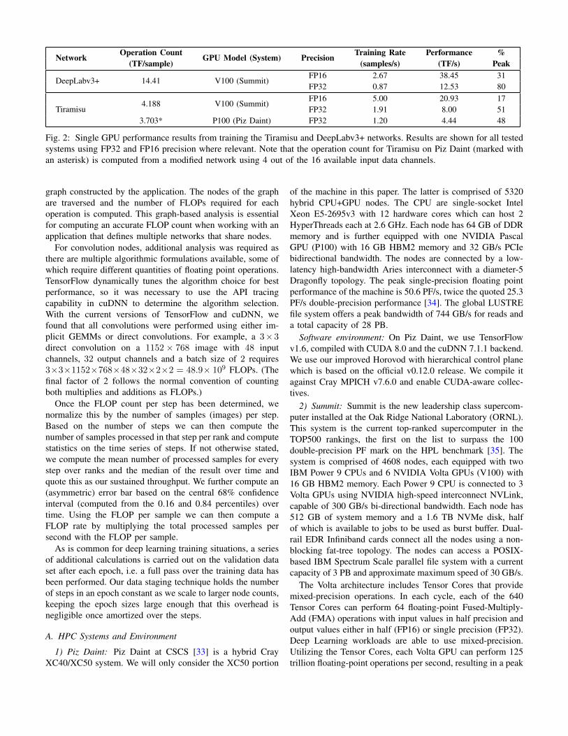
Network Operation Count GPU Model (System) Precision Training Rate Performance %(TF/sample) (samples/s) (TF/s) Peak
DeepLabv3+ 14.41 V100 (Summit)FP16 2.67 38.45 31FP32 0.87 12.53 80
Tiramisu4.188 V100 (Summit)
FP16 5.00 20.93 17FP32 1.91 8.00 51
3.703* P100 (Piz Daint) FP32 1.20 4.44 48
Fig. 2: Single GPU performance results from training the Tiramisu and DeepLabv3+ networks. Results are shown for all testedsystems using FP32 and FP16 precision where relevant. Note that the operation count for Tiramisu on Piz Daint (marked withan asterisk) is computed from a modified network using 4 out of the 16 available input data channels.
graph constructed by the application. The nodes of the graphare traversed and the number of FLOPs required for eachoperation is computed. This graph-based analysis is essentialfor computing an accurate FLOP count when working with anapplication that defines multiple networks that share nodes.
For convolution nodes, additional analysis was required asthere are multiple algorithmic formulations available, some ofwhich require different quantities of floating point operations.TensorFlow dynamically tunes the algorithm choice for bestperformance, so it was necessary to use the API tracingcapability in cuDNN to determine the algorithm selection.With the current versions of TensorFlow and cuDNN, wefound that all convolutions were performed using either im-plicit GEMMs or direct convolutions. For example, a 3×3direct convolution on a 1152 × 768 image with 48 inputchannels, 32 output channels and a batch size of 2 requires3×3×1152×768×48×32×2×2 = 48.9× 10⁹ FLOPs. (Thefinal factor of 2 follows the normal convention of countingboth multiplies and additions as FLOPs.)
Once the FLOP count per step has been determined, wenormalize this by the number of samples (images) per step.Based on the number of steps we can then compute thenumber of samples processed in that step per rank and computestatistics on the time series of steps. If not otherwise stated,we compute the mean number of processed samples for everystep over ranks and the median of the result over time andquote this as our sustained throughput. We further compute an(asymmetric) error bar based on the central 68% confidenceinterval (computed from the 0.16 and 0.84 percentiles) overtime. Using the FLOP per sample we can then compute aFLOP rate by multiplying the total processed samples persecond with the FLOP per sample.
As is common for deep learning training situations, a seriesof additional calculations is carried out on the validation dataset after each epoch, i.e. a full pass over the training data hasbeen performed. Our data staging technique holds the numberof steps in an epoch constant as we scale to larger node counts,keeping the epoch sizes large enough that this overhead isnegligible once amortized over the steps.
A. HPC Systems and Environment
1) Piz Daint: Piz Daint at CSCS [33] is a hybrid CrayXC40/XC50 system. We will only consider the XC50 portion
of the machine in this paper. The latter is comprised of 5320hybrid CPU+GPU nodes. The CPU are single-socket IntelXeon E5-2695v3 with 12 hardware cores which can host 2HyperThreads each at 2.6 GHz. Each node has 64 GB of DDRmemory and is further equipped with one NVIDIA PascalGPU (P100) with 16 GB HBM2 memory and 32 GB/s PCIebidirectional bandwidth. The nodes are connected by a low-latency high-bandwidth Aries interconnect with a diameter-5Dragonfly topology. The peak single-precision floating pointperformance of the machine is 50.6 PF/s, twice the quoted 25.3PF/s double-precision performance [34]. The global LUSTREfile system offers a peak bandwidth of 744 GB/s for reads anda total capacity of 28 PB.
Software environment: On Piz Daint, we use TensorFlowv1.6, compiled with CUDA 8.0 and the cuDNN 7.1.1 backend.We use our improved Horovod with hierarchical control planewhich is based on the official v0.12.0 release. We compile itagainst Cray MPICH v7.6.0 and enable CUDA-aware collec-tives.
2) Summit: Summit is the new leadership class supercom-puter installed at the Oak Ridge National Laboratory (ORNL).This system is the current top-ranked supercomputer in theTOP500 rankings, the first on the list to surpass the 100double-precision PF mark on the HPL benchmark [35]. Thesystem is comprised of 4608 nodes, each equipped with twoIBM Power 9 CPUs and 6 NVIDIA Volta GPUs (V100) with16 GB HBM2 memory. Each Power 9 CPU is connected to 3Volta GPUs using NVIDIA high-speed interconnect NVLink,capable of 300 GB/s bi-directional bandwidth. Each node has512 GB of system memory and a 1.6 TB NVMe disk, halfof which is available to jobs to be used as burst buffer. Dual-rail EDR Infiniband cards connect all the nodes using a non-blocking fat-tree topology. The nodes can access a POSIX-based IBM Spectrum Scale parallel file system with a currentcapacity of 3 PB and approximate maximum speed of 30 GB/s.
The Volta architecture includes Tensor Cores that providemixed-precision operations. In each cycle, each of the 640Tensor Cores can perform 64 floating-point Fused-Multiply-Add (FMA) operations with input values in half precision andoutput values either in half (FP16) or single precision (FP32).Deep Learning workloads are able to use mixed-precision.Utilizing the Tensor Cores, each Volta GPU can perform 125trillion floating-point operations per second, resulting in a peak
Tiramisu DeepLabv3+FP32 Training FP16 Training FP32 Training FP16 Training
Category #Kern
%Time
%Math
%Mem
#Kern
%Time
%Math
%Mem
#Kern
%Time
%Math
%Mem
#Kern
%Time
%Math
%Mem
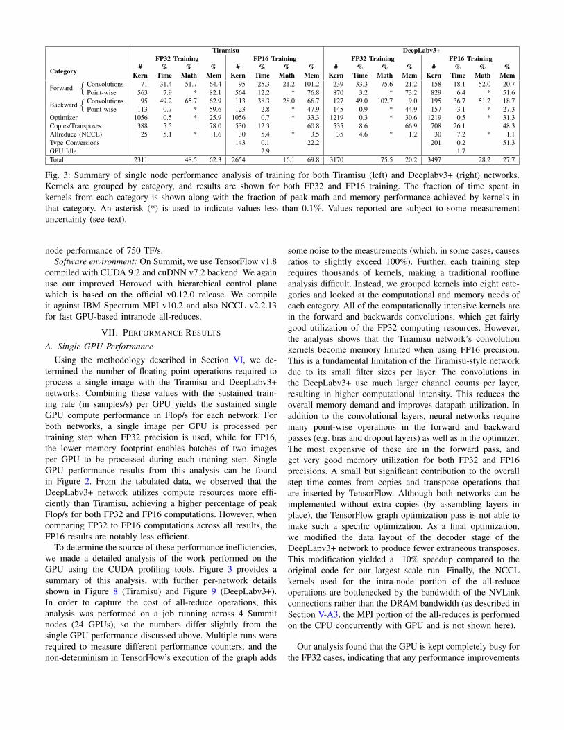
Forward{ Convolutions 71 31.4 51.7 64.4 95 25.3 21.2 101.2 239 33.3 75.6 21.2 158 18.1 52.0 20.7
Point-wise 563 7.9 * 82.1 564 12.2 * 76.8 870 3.2 * 73.2 829 6.4 * 51.6
Backward{ Convolutions 95 49.2 65.7 62.9 113 38.3 28.0 66.7 127 49.0 102.7 9.0 195 36.7 51.2 18.7
Point-wise 113 0.7 * 59.6 123 2.8 * 47.9 145 0.9 * 44.9 157 3.1 * 27.3Optimizer 1056 0.5 * 25.9 1056 0.7 * 33.3 1219 0.3 * 30.6 1219 0.5 * 31.3Copies/Transposes 388 5.5 78.0 530 12.3 60.8 535 8.6 66.9 708 26.1 48.3Allreduce (NCCL) 25 5.1 * 1.6 30 5.4 * 3.5 35 4.6 * 1.2 30 7.2 * 1.1Type Conversions 143 0.1 22.2 201 0.2 51.3GPU Idle 2.9 1.7Total 2311 48.5 62.3 2654 16.1 69.8 3170 75.5 20.2 3497 28.2 27.7
Fig. 3: Summary of single node performance analysis of training for both Tiramisu (left) and Deeplabv3+ (right) networks.Kernels are grouped by category, and results are shown for both FP32 and FP16 training. The fraction of time spent inkernels from each category is shown along with the fraction of peak math and memory performance achieved by kernels inthat category. An asterisk (*) is used to indicate values less than 0.1%. Values reported are subject to some measurementuncertainty (see text).
node performance of 750 TF/s.Software environment: On Summit, we use TensorFlow v1.8
compiled with CUDA 9.2 and cuDNN v7.2 backend. We againuse our improved Horovod with hierarchical control planewhich is based on the official v0.12.0 release. We compileit against IBM Spectrum MPI v10.2 and also NCCL v2.2.13for fast GPU-based intranode all-reduces.
VII. PERFORMANCE RESULTS
A. Single GPU Performance
Using the methodology described in Section VI, we de-termined the number of floating point operations required toprocess a single image with the Tiramisu and DeepLabv3+networks. Combining these values with the sustained train-ing rate (in samples/s) per GPU yields the sustained singleGPU compute performance in Flop/s for each network. Forboth networks, a single image per GPU is processed pertraining step when FP32 precision is used, while for FP16,the lower memory footprint enables batches of two imagesper GPU to be processed during each training step. SingleGPU performance results from this analysis can be foundin Figure 2. From the tabulated data, we observed that theDeepLabv3+ network utilizes compute resources more effi-ciently than Tiramisu, achieving a higher percentage of peakFlop/s for both FP32 and FP16 computations. However, whencomparing FP32 to FP16 computations across all results, theFP16 results are notably less efficient.
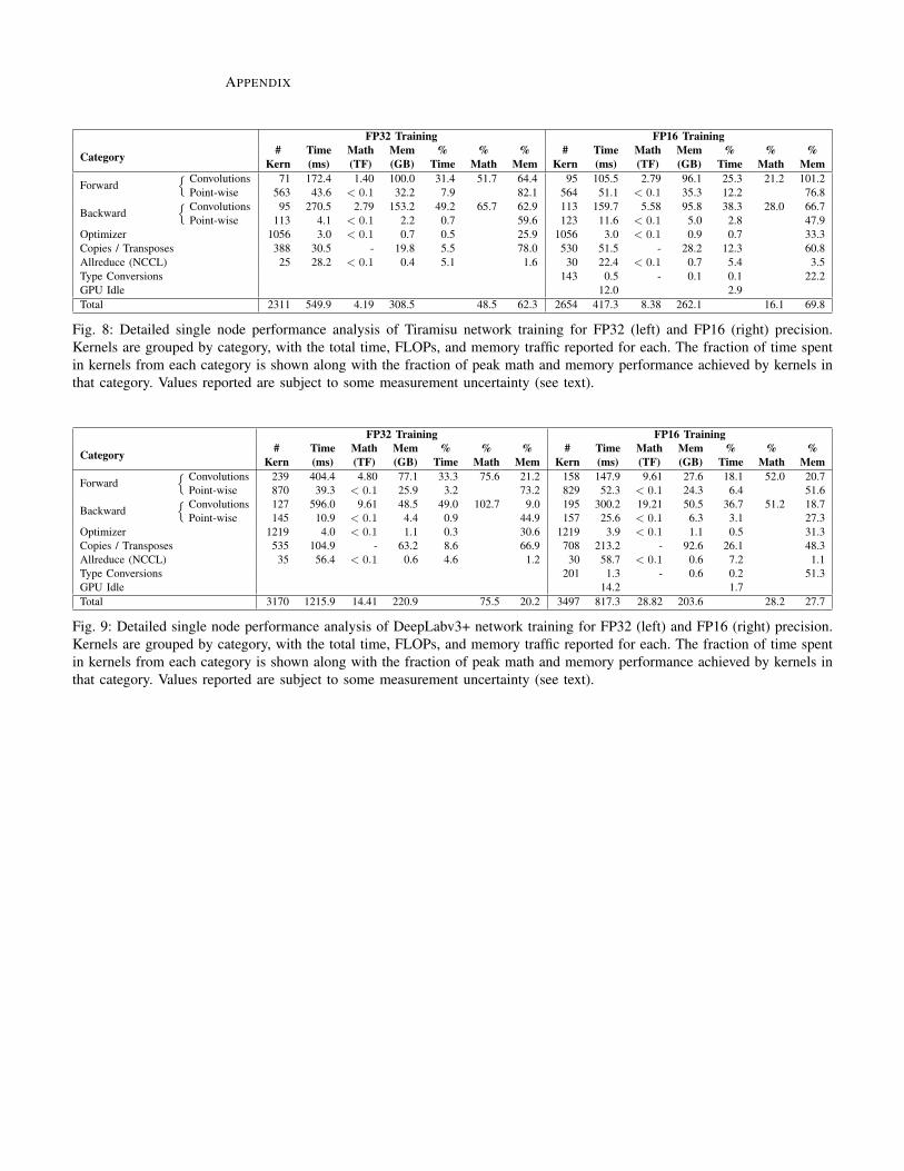
To determine the source of these performance inefficiencies,we made a detailed analysis of the work performed on theGPU using the CUDA profiling tools. Figure 3 provides asummary of this analysis, with further per-network detailsshown in Figure 8 (Tiramisu) and Figure 9 (DeepLabv3+).In order to capture the cost of all-reduce operations, thisanalysis was performed on a job running across 4 Summitnodes (24 GPUs), so the numbers differ slightly from thesingle GPU performance discussed above. Multiple runs wererequired to measure different performance counters, and thenon-determinism in TensorFlow’s execution of the graph adds
some noise to the measurements (which, in some cases, causesratios to slightly exceed 100%). Further, each training steprequires thousands of kernels, making a traditional rooflineanalysis difficult. Instead, we grouped kernels into eight cate-gories and looked at the computational and memory needs ofeach category. All of the computationally intensive kernels arein the forward and backwards convolutions, which get fairlygood utilization of the FP32 computing resources. However,the analysis shows that the Tiramisu network’s convolutionkernels become memory limited when using FP16 precision.This is a fundamental limitation of the Tiramisu-style networkdue to its small filter sizes per layer. The convolutions inthe DeepLabv3+ use much larger channel counts per layer,resulting in higher computational intensity. This reduces theoverall memory demand and improves datapath utilization. Inaddition to the convolutional layers, neural networks requiremany point-wise operations in the forward and backwardpasses (e.g. bias and dropout layers) as well as in the optimizer.The most expensive of these are in the forward pass, andget very good memory utilization for both FP32 and FP16precisions. A small but significant contribution to the overallstep time comes from copies and transpose operations thatare inserted by TensorFlow. Although both networks can beimplemented without extra copies (by assembling layers inplace), the TensorFlow graph optimization pass is not able tomake such a specific optimization. As a final optimization,we modified the data layout of the decoder stage of theDeepLapv3+ network to produce fewer extraneous transposes.This modification yielded a 10% speedup compared to theoriginal code for our largest scale run. Finally, the NCCLkernels used for the intra-node portion of the all-reduceoperations are bottlenecked by the bandwidth of the NVLinkconnections rather than the DRAM bandwidth (as described inSection V-A3, the MPI portion of the all-reduces is performedon the CPU concurrently with GPU and is not shown here).
Our analysis found that the GPU is kept completely busy forthe FP32 cases, indicating that any performance improvements
have to come from optimizing or eliminating some of thekernels running on the GPU. The most beneficial kernels tooptimize are the convolutions, but with so many differentkernels being used, the effort would be significant, and woulddeny the application the benefit of any improvements thatare made to the cuDNN library. For example, a move fromcuDNN v7.0.5 to v7.1.2 early in the project resulted in a 5%performance improvement with no changes to the application.We explored a move away from TensorFlow, implementing thenetwork directly with cuDNN library calls, but the resultingcode was much harder to maintain than the TensorFlow ver-sion. A 5-10% performance gain was not worth the impact onprogrammer productivity. The final optimization strategy, andthe one we are pursuing, is to make incremental improvementswithin TensorFlow to improve the memory management andfuse some of the point-wise operations together to reduce thenumber of times tensors are read and written to DRAM. Thismight also allow the batch size to be increased, which wouldalso improve the efficiency of the convolutional stages.
With the use of significantly faster math in the FP16 cases,the memory-bound kernels consume a larger fraction of theoverall step time, and any optimizations to eliminate copies orfuse point-wise tasks will help the FP16 even more than FP32.The profile for the FP16 also shows some periods where theGPU has run out of work, suggesting that code running on theCPU such as the input pipeline or the TensorFlow schedulermay require additional optimization as well.
B. Scaling Experiments
We perform several scaling experiments on Piz Daint andSummit. On Piz Daint, we ran the Tiramisu network only,while on Summit, both Tiramisu and DeepLabv3+ networkswere run. The experiment setup is slightly different for thetwo systems and we explain the details below. We bind oneMPI rank to each GPU which amounts to one rank per nodeon Piz Daint and six ranks per node on Summit.
On Piz Daint, we scale the training up from a single GPU tothe full machine, i.e. 5300 nodes. We also compare the scalingbehavior when staging input data against reading it from theglobal Lustre file system. On Summit, we run with a singleGPU as a baseline, but then sweep from 1 to 4560 nodes usingall 6 GPUs per node (i.e. 6 to 27360 GPUs).
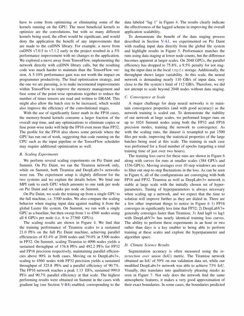
The scaling results are shown in Figure 4. We find thatthe training performance of Tiramisu scales to a sustained21.0 PF/s on the full Piz Daint machine, achieving parallelefficiencies of 83.4% at 2048 nodes and 79.0% at 5300 nodesin FP32. On Summit, scaling Tiramisu to 4096 nodes yields asustained throughput of 176.8 PF/s and 492.2 PF/s for FP32and FP16 precision respectively, maintaining parallel efficien-cies above 90% in both cases. Moving on to DeepLabv3+,scaling to 4560 nodes with FP32 precision yields a sustainedthroughput of 325.8 PF/s and a parallel efficiency of 90.7%.The FP16 network reaches a peak 1.13 EF/s, sustained 999.0PF/s and 90.7% parallel efficiency at that scale. The highestperforming results were obtained on Summit in the cases withgradient lag (see Section V-B4) enabled, corresponding to the
data labeled “lag 1" in Figure 4. The results clearly indicatethe effectiveness of the lagged scheme in improving the overallapplication scalability.
To demonstrate the benefit of the data staging processdescribed in Section V-A1, we experimented on Piz Daintwith reading input data directly from the global file systemand highlight results in Figure 5. Performance matches theruns using data staging at lower node counts, but the differencebecomes apparent at larger scales. On 2048 GPUs, the parallelefficiency has dropped to 75.8%, a 9.5% penalty for not stag-ing the input data in the local tmpfs storage. Additionally, thethroughput shows larger variability. At this scale, the neuralnetwork is demanding nearly 110 GB/s of input data, veryclose to the file system’s limit of 112 GB/s. Therefore, we didnot attempt to scale beyond 2048 nodes without data staging.
C. Convergence at Scale
A major challenge for deep neural networks is to main-tain convergence properties (and with good accuracy) as thenetwork training is scaled out. To demonstrate the stabilityof our network at large scales, we performed longer runs onup to 1024 Summit nodes using both the FP32 and FP16precision modes, training the network to convergence. Aswith the scaling runs, the dataset is resampled to put 1500files per node, improving the statistical properties of the largebatches being used at this scale. The training in each casewas performed for a fixed number of epochs (targeting a totaltraining time of just over two hours).
The training loss curve for these runs are shown in Figure 6along with curves for runs at smaller scales (384 GPUs and1536 GPUs). Moving averages over 10 step windows are usedto filter out step-to-step fluctuations in the loss. As can be seenin Figure 6, all of the configurations are converging with bothFP16 and FP32. Tiramisu as well as DeepLabv3+ network isstable at large scale with the initially chosen set of hyper-parameters. Tuning of hyperparameters is always necessarywhen scaling up a network, and we expect that the time tosolution will improve further as they are dialed in. There area few other important things to notice in Figure 6 1) FP16converges in significantly less time that FP32; 2) DeepLabV3+generally converges faster than Tiramisu; 3) And lag0 vs lag1with DeepLabV3+ has nearly identical training loss curves.The ability to perform these experiments in an hour or tworather than days is a key enabler to being able to performtraining at these scales and explore the hyperparameter andalgorithm space.
D. Climate Science Results
Segmentation accuracy is often measured using the in-tersection over union (IoU) metric. The Tiramisu networkobtained an IoU of 59% on our validation data set, while ourmodified DeepLabv3+ network was able to achieve 73% IoU.Visually, this translates into qualitatively pleasing masks asseen in Figure 7. Not only does the network find the sameatmospheric features, it makes a very good approximation oftheir exact boundaries. In some cases, the boundaries predicted
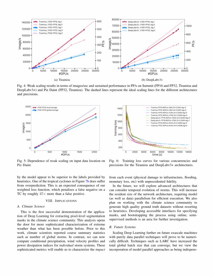
(a) Tiramisu (b) DeepLabv3+
Fig. 4: Weak scaling results in terms of images/sec and sustained performance in PF/s on Summit (FP16 and FP32, Tiramisu andDeepLabv3+) and Piz Daint (FP32, Tiramisu). The dashed lines represent the ideal scaling lines for the different architecturesand precisions.
0 500 1000 1500 2000#GPUs
0
500
1000
1500
2000
2500
imag
e/s
P100-FP32 local storageP100-FP32 global storage
Fig. 5: Dependence of weak scaling on input data location onPiz Daint.
by the model appear to be superior to the labels provided byheuristics. One of the tropical cyclones in Figure 7b does sufferfrom overprediction. This is an expected consequence of ourweighted loss function, which penalizes a false negative on aTC by roughly 37× more than a false positive.
VIII. IMPLICATIONS
A. Climate Science
This is the first successful demonstration of the applica-tion of Deep Learning for extracting pixel-level segmentationmasks in the climate science community. This analysis opensthe door for more sophisticated characterization of extremeweather than what has been possible before. Prior to thiswork, climate scientists reported coarse summary statisticssuch as number of global storms. In contrast, we can nowcompute conditional precipitation, wind velocity profiles andpower dissipation indices for individual storm systems. Thesesophisticated metrics will enable us to characterize the impact
0 2000 4000 6000 8000 10000 12000 14000time [s]
200
400
600
800
1000
1200
1400
trai
ning
loss
Tiramisu FP16 #GPUs=384 LR=0.0001 lag=0Tiramisu FP32 #GPUs=384 LR=0.0001 lag=0Tiramisu FP16 #GPUs=1536 LR=0.0064 lag=0Tiramisu FP32 #GPUs=1536 LR=0.0064 lag=0DeepLabv3+ FP16 #GPUs=1536 LR=0.0064 lag=0DeepLabv3+ FP16 #GPUs=1536 LR=0.0064 lag=1Tiramisu FP16 #GPUs=6144 LR=0.4096 lag=0Tiramisu FP32 #GPUs=6144 LR=0.4096 lag=0
Fig. 6: Training loss curves for various concurrencies andprecisions for the Tiramisu and DeepLabv3+ architectures.
from each event (physical damage to infrastructure, flooding,monetary loss, etc) with unprecedented fidelity.
In the future, we will explore advanced architectures thatcan consider temporal evolution of storms. This will increasethe resident size of the network architecture, requiring model(as well as data) parallelism for efficient execution. We alsoplan on working with the climate science community togenerate high quality ground truth datasets without resortingto heuristics. Developing accessible interfaces for specifyingmasks, and bootstrapping the process using online, semi-supervised methods is an area for further investigation.
B. Future Systems
Scaling Deep Learning further on future exascale machineswith purely data parallel techniques will prove to be numeri-cally difficult. Techniques such as LARC have increased thetotal global batch size that can converge, but we view theincorporation of model parallel approaches as being indispens-
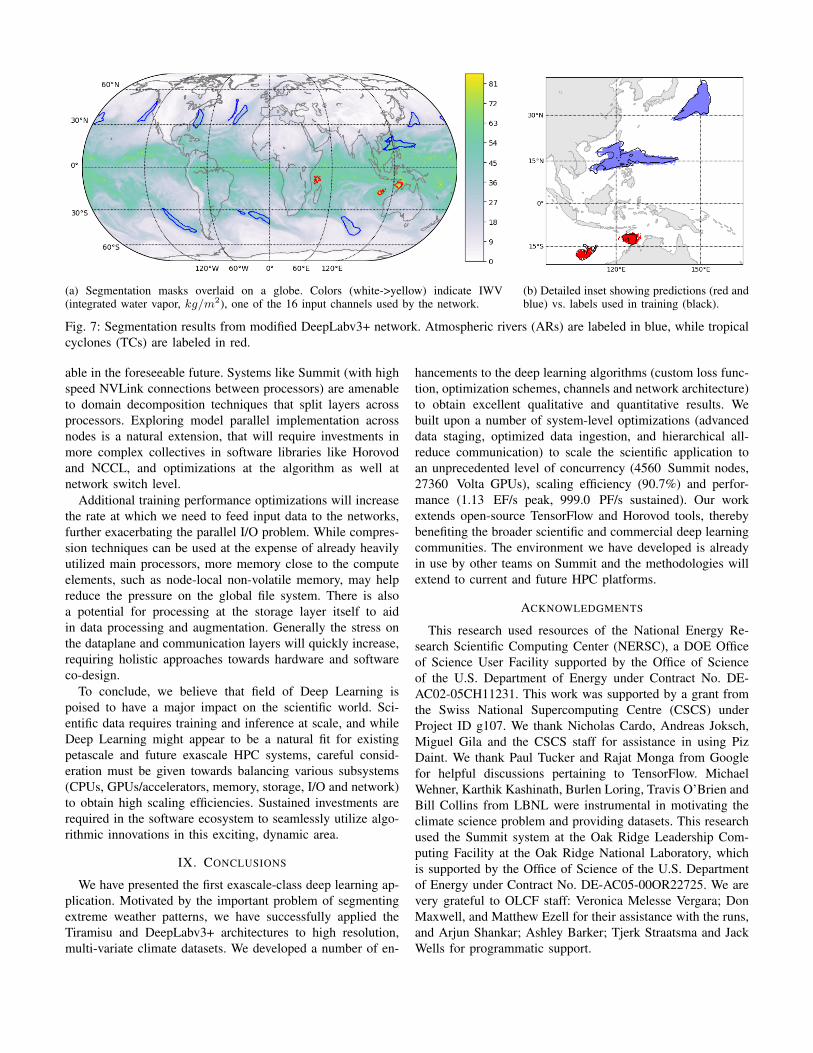
(a) Segmentation masks overlaid on a globe. Colors (white->yellow) indicate IWV(integrated water vapor, kg/m2), one of the 16 input channels used by the network.
(b) Detailed inset showing predictions (red andblue) vs. labels used in training (black).
Fig. 7: Segmentation results from modified DeepLabv3+ network. Atmospheric rivers (ARs) are labeled in blue, while tropicalcyclones (TCs) are labeled in red.
able in the foreseeable future. Systems like Summit (with highspeed NVLink connections between processors) are amenableto domain decomposition techniques that split layers acrossprocessors. Exploring model parallel implementation acrossnodes is a natural extension, that will require investments inmore complex collectives in software libraries like Horovodand NCCL, and optimizations at the algorithm as well atnetwork switch level.
Additional training performance optimizations will increasethe rate at which we need to feed input data to the networks,further exacerbating the parallel I/O problem. While compres-sion techniques can be used at the expense of already heavilyutilized main processors, more memory close to the computeelements, such as node-local non-volatile memory, may helpreduce the pressure on the global file system. There is alsoa potential for processing at the storage layer itself to aidin data processing and augmentation. Generally the stress onthe dataplane and communication layers will quickly increase,requiring holistic approaches towards hardware and softwareco-design.
To conclude, we believe that field of Deep Learning ispoised to have a major impact on the scientific world. Sci-entific data requires training and inference at scale, and whileDeep Learning might appear to be a natural fit for existingpetascale and future exascale HPC systems, careful consid-eration must be given towards balancing various subsystems(CPUs, GPUs/accelerators, memory, storage, I/O and network)to obtain high scaling efficiencies. Sustained investments arerequired in the software ecosystem to seamlessly utilize algo-rithmic innovations in this exciting, dynamic area.
IX. CONCLUSIONS
We have presented the first exascale-class deep learning ap-plication. Motivated by the important problem of segmentingextreme weather patterns, we have successfully applied theTiramisu and DeepLabv3+ architectures to high resolution,multi-variate climate datasets. We developed a number of en-
hancements to the deep learning algorithms (custom loss func-tion, optimization schemes, channels and network architecture)to obtain excellent qualitative and quantitative results. Webuilt upon a number of system-level optimizations (advanceddata staging, optimized data ingestion, and hierarchical all-reduce communication) to scale the scientific application toan unprecedented level of concurrency (4560 Summit nodes,27360 Volta GPUs), scaling efficiency (90.7%) and perfor-mance (1.13 EF/s peak, 999.0 PF/s sustained). Our workextends open-source TensorFlow and Horovod tools, therebybenefiting the broader scientific and commercial deep learningcommunities. The environment we have developed is alreadyin use by other teams on Summit and the methodologies willextend to current and future HPC platforms.
ACKNOWLEDGMENTS
This research used resources of the National Energy Re-search Scientific Computing Center (NERSC), a DOE Officeof Science User Facility supported by the Office of Scienceof the U.S. Department of Energy under Contract No. DE-AC02-05CH11231. This work was supported by a grant fromthe Swiss National Supercomputing Centre (CSCS) underProject ID g107. We thank Nicholas Cardo, Andreas Joksch,Miguel Gila and the CSCS staff for assistance in using PizDaint. We thank Paul Tucker and Rajat Monga from Googlefor helpful discussions pertaining to TensorFlow. MichaelWehner, Karthik Kashinath, Burlen Loring, Travis O’Brien andBill Collins from LBNL were instrumental in motivating theclimate science problem and providing datasets. This researchused the Summit system at the Oak Ridge Leadership Com-puting Facility at the Oak Ridge National Laboratory, whichis supported by the Office of Science of the U.S. Departmentof Energy under Contract No. DE-AC05-00OR22725. We arevery grateful to OLCF staff: Veronica Melesse Vergara; DonMaxwell, and Matthew Ezell for their assistance with the runs,and Arjun Shankar; Ashley Barker; Tjerk Straatsma and JackWells for programmatic support.
REFERENCES
[1] Prabhat, O. Ruebel, S. Byna, K. Wu, F. Li, M. Wehner, and W. Bethel,“Teca: A parallel toolkit for extreme climate analysis,” Procedia Com-puter Science, vol. 9, pp. 866 – 876, 2012, proceedings of ICCS 2012.
[2] Y. Liu, E. Racah, Prabhat, J. Correa, A. Khosrowshahi, D. Lavers,K. Kunkel, M. Wehner, and W. Collins, “Application of deep con-volutional neural networks for detecting extreme weather in climatedatasets,” arXiv preprint arXiv:1605.01156, 2016.
[3] S. Hong, S. Kim, M. Joh, and S.-k. Song, “Globenet: Convolutionalneural networks for typhoon eye tracking from remote sensing imagery,”arXiv preprint arXiv:1708.03417, 2017.
[4] E. Racah, C. Beckham, T. Maharaj, S. Ebrahimi Kahou, Prabhat, andC. Pal, “Extreme weather: A large-scale climate dataset for semi-supervised detection, localization, and understanding of extreme weatherevents,” in Advances in Neural Information Processing Systems 30, 2017.
[5] M. Abadi, A. Agarwal, P. Barham, E. Brevdo, Z. Chen, C. Citro, G. S.Corrado, A. Davis, J. Dean, M. Devin, S. Ghemawat, I. Goodfellow,A. Harp, G. Irving, M. Isard, Y. Jia, R. Jozefowicz, L. Kaiser,M. Kudlur, J. Levenberg, D. Mané, R. Monga, S. Moore, D. Murray,C. Olah, M. Schuster, J. Shlens, B. Steiner, I. Sutskever, K. Talwar,P. Tucker, V. Vanhoucke, V. Vasudevan, F. Viégas, O. Vinyals,P. Warden, M. Wattenberg, M. Wicke, Y. Yu, and X. Zheng,“TensorFlow: Large-scale machine learning on heterogeneous systems,”2015, software available from tensorflow.org. [Online]. Available:https://www.tensorflow.org/
[6] TensorFlow website. [Online]. Available: https://tensorflow.org[7] S. Jégou, M. Drozdzal, D. Vazquez, A. Romero, and Y. Bengio, “The
one hundred layers tiramisu: Fully convolutional densenets for semanticsegmentation,” in Computer Vision and Pattern Recognition Workshops(CVPRW), 2017 IEEE Conference on. IEEE, 2017, pp. 1175–1183.
[8] K. He, X. Zhang, S. Ren, and J. Sun, “Deep residual learning for imagerecognition,” in Proceedings of the IEEE conference on computer visionand pattern recognition, 2016, pp. 770–778.
[9] D. P. Kingma and J. Ba, “Adam: A method for stochastic optimization,”arXiv preprint arXiv:1412.6980, 2014.
[10] L.-C. Chen, Y. Zhu, G. Papandreou, F. Schroff, and H. Adam, “Encoder-decoder with atrous separable convolution for semantic image segmen-tation,” in ECCV, 2018.
[11] Prabhat, S. Byna, V. Vishwanath, E. Dart, M. Wehner, and W. D. Collins,“Teca: Petascale pattern recognition for climate science,” in ComputerAnalysis of Images and Patterns, 2015, pp. 426–436.
[12] C. A. Shields, J. J. Rutz, L.-Y. Leung, F. M. Ralph, M. Wehner,B. Kawzenuk, J. M. Lora, E. McClenny, T. Osborne, A. E. Payneet al., “Atmospheric river tracking method intercomparison project(artmip): project goals and experimental design,” Geoscientific ModelDevelopment, vol. 11, no. 6, pp. 2455–2474, 2018.
[13] Prabhat, “Deep learning for science,” https://www.oreilly.com/ideas/a-look-at-deep-learning-for-science, 2017.
[14] A. Radovic, M. Williams, D. Rousseau, M. Kagan, D. Bonacorsi,A. Himmel, A. Aurisano, K. Terao, and T. Wongjirad, “Machine learningat the energy and intensity frontiers of particle physics,” Nature, 2018.
[15] A. Mathuriya et al., “CosmoFlow: Using Deep Learning to Learn theUniverse at Scale,” in Proceedings of SuperComputing, 2018.
[16] R. Gómez-Bombarelli, D. K. Duvenaud, J. M. Hernández-Lobato,J. Aguilera-Iparraguirre, T. D. Hirzel, R. P. Adams, and A. Aspuru-Guzik, “Automatic chemical design using a data-driven continuousrepresentation of molecules,” CoRR, vol. abs/1610.02415, 2016.[Online]. Available: http://arxiv.org/abs/1610.02415
[17] D. George and E. A. Huerta, “Deep neural networks to enable real-timemultimessenger astrophysics,” Phys. Rev. D, vol. 97, p. 044039, Feb2018.
[18] J. Regier, Prabhat, and J. McAuliffe, “A deep generative model forastronomical images of galaxies,” in NIPS Workshop: Advances inApproximate Bayesian Inference, 2015.
[19] A. Karpatne and V. Kumar, “Big data in climate: Opportunities andchallenges for machine learning,” in Proceedings of the 23rd ACMSIGKDD International Conference on Knowledge Discovery and DataMining, ser. KDD ’17. New York, NY, USA: ACM, 2017, pp. 21–22.[Online]. Available: http://doi.acm.org/10.1145/3097983.3105810
[20] O. Hennigh, “Lat-Net: Compressing Lattice Boltzmann Flow Simula-tions using Deep Neural Networks,” ArXiv e-prints, May 2017.
[21] J.-X. Wang, J. Wu, J. Ling, G. Iaccarino, and H. Xiao, “A Compre-hensive Physics-Informed Machine Learning Framework for PredictiveTurbulence Modeling,” ArXiv e-prints, Jan. 2017.
[22] W. S. McCulloch and W. Pitts, “A logical calculus of the ideas immanentin nervous activity,” The bulletin of mathematical biophysics, vol. 5,no. 4, pp. 115–133, 1943.
[23] F. Rosenblatt, “The perceptron: a probabilistic model for informationstorage and organization in the brain.” Psychological review, vol. 65,no. 6, p. 386, 1958.
[24] A. Krizhevsky, I. Sutskever, and G. E. Hinton, “Imagenet classificationwith deep convolutional neural networks,” in Advances in neural infor-mation processing systems, 2012, pp. 1097–1105.
[25] T. Akiba, K. Fukuda, and S. Suzuki, “ChainerMN: ScalableDistributed Deep Learning Framework,” in Proceedings of Workshopon ML Systems in The Thirty-first Annual Conference on NeuralInformation Processing Systems (NIPS), 2017. [Online]. Available:http://learningsys.org/nips17/assets/papers/paper_25.pdf
[26] T. Akiba, S. Suzuki, and K. Fukuda, “Extremely large minibatchsgd: Training resnet-50 on imagenet in 15 minutes,” 2017. [Online].Available: https://www.preferred-networks.jp/docs/imagenet_in_15min.pdf
[27] X. Jia, S. Song, W. He, Y. Wang, H. Rong, F. Zhou, L. Xie, Z. Guo,Y. Yang, L. Yu, T. Chen, G. Hu, S. Shi, and X. Chu, “HighlyScalable Deep Learning Training System with Mixed-Precision: TrainingImageNet in Four Minutes,” ArXiv e-prints, Jul. 2018.
[28] A. Sergeev and M. D. Balso, “Horovod: fast and easy distributed deeplearning in TensorFlow,” arXiv preprint arXiv:1802.05799, 2018.
[29] NVIDIA Collective Communications Library (NCCL). [Online].Available: https://developer.nvidia.com/nccl
[30] B. Ginsburg, I. Gitman, and O. Kuchaiev, “Layer-Wise Adaptive RateControl for Training of Deep Networks,” in preparation, 2018.
[31] Y. You, I. Gitman, and B. Ginsburg, “Large Batch Training of Convo-lutional Networks,” ArXiv e-prints, Aug. 2017.
[32] S. Zhang, A. Choromanska, and Y. LeCun, “Deep learning with elasticaveraging SGD,” CoRR, vol. abs/1412.6651, 2014. [Online]. Available:http://arxiv.org/abs/1412.6651
[33] Piz Daint | CSCS. [Online]. Available: https://www.cscs.ch/computers/piz-daint/
[34] Piz Daint - Cray XC50, Xeon E5-2690v3 12C 2.6GHz, Aries intercon-nect, NVIDIA Tesla P100 | TOP500 Supercomputer Sites.
[35] Summit - IBM Power System AC922, IBM POWER9 22C 3.07GHz,NVIDIA Volta GV100, Dual-rail Mellanox EDR Infiniband | TOP500Supercomputer Sites. [Online]. Available: https://www.top500.org/system/179397
APPENDIX
FP32 Training FP16 Training
Category #Kern
Time(ms)
Math(TF)
Mem(GB)
%Time
%Math
%Mem
#Kern
Time(ms)
Math(TF)
Mem(GB)
%Time
%Math
%Mem
Forward{ Convolutions 71 172.4 1.40 100.0 31.4 51.7 64.4 95 105.5 2.79 96.1 25.3 21.2 101.2
Point-wise 563 43.6 < 0.1 32.2 7.9 82.1 564 51.1 < 0.1 35.3 12.2 76.8
Backward{ Convolutions 95 270.5 2.79 153.2 49.2 65.7 62.9 113 159.7 5.58 95.8 38.3 28.0 66.7
Point-wise 113 4.1 < 0.1 2.2 0.7 59.6 123 11.6 < 0.1 5.0 2.8 47.9Optimizer 1056 3.0 < 0.1 0.7 0.5 25.9 1056 3.0 < 0.1 0.9 0.7 33.3Copies / Transposes 388 30.5 - 19.8 5.5 78.0 530 51.5 - 28.2 12.3 60.8Allreduce (NCCL) 25 28.2 < 0.1 0.4 5.1 1.6 30 22.4 < 0.1 0.7 5.4 3.5Type Conversions 143 0.5 - 0.1 0.1 22.2GPU Idle 12.0 2.9Total 2311 549.9 4.19 308.5 48.5 62.3 2654 417.3 8.38 262.1 16.1 69.8
Fig. 8: Detailed single node performance analysis of Tiramisu network training for FP32 (left) and FP16 (right) precision.Kernels are grouped by category, with the total time, FLOPs, and memory traffic reported for each. The fraction of time spentin kernels from each category is shown along with the fraction of peak math and memory performance achieved by kernels inthat category. Values reported are subject to some measurement uncertainty (see text).
FP32 Training FP16 Training
Category #Kern
Time(ms)
Math(TF)
Mem(GB)
%Time
%Math
%Mem
#Kern
Time(ms)
Math(TF)
Mem(GB)
%Time
%Math
%Mem
Forward{ Convolutions 239 404.4 4.80 77.1 33.3 75.6 21.2 158 147.9 9.61 27.6 18.1 52.0 20.7
Point-wise 870 39.3 < 0.1 25.9 3.2 73.2 829 52.3 < 0.1 24.3 6.4 51.6
Backward{ Convolutions 127 596.0 9.61 48.5 49.0 102.7 9.0 195 300.2 19.21 50.5 36.7 51.2 18.7
Point-wise 145 10.9 < 0.1 4.4 0.9 44.9 157 25.6 < 0.1 6.3 3.1 27.3Optimizer 1219 4.0 < 0.1 1.1 0.3 30.6 1219 3.9 < 0.1 1.1 0.5 31.3Copies / Transposes 535 104.9 - 63.2 8.6 66.9 708 213.2 - 92.6 26.1 48.3Allreduce (NCCL) 35 56.4 < 0.1 0.6 4.6 1.2 30 58.7 < 0.1 0.6 7.2 1.1Type Conversions 201 1.3 - 0.6 0.2 51.3GPU Idle 14.2 1.7Total 3170 1215.9 14.41 220.9 75.5 20.2 3497 817.3 28.82 203.6 28.2 27.7
Fig. 9: Detailed single node performance analysis of DeepLabv3+ network training for FP32 (left) and FP16 (right) precision.Kernels are grouped by category, with the total time, FLOPs, and memory traffic reported for each. The fraction of time spentin kernels from each category is shown along with the fraction of peak math and memory performance achieved by kernels inthat category. Values reported are subject to some measurement uncertainty (see text).