1. You’ll need to download whatever the current sheet is (at the moment it’s the last one I put up)

2. Once downloaded and open, edit all the things you’re going to edit, it will make dealing with the pictures easier if you do these

last.

3. The first method is to simply insert an image. To do this you need to use the tool ribbon to open the insert menu.

4. Next you’ll find the insert picture option in this menu.

5. You can then find your image and place it in the correct area. These images will float and therefore be susceptible to people

moving them in the future by accident and when cell sizes change, but this makes them easy to move, resize, and to insert into

the file.

6. The second method is more detailed and will involve editing your image before placing it into the cell, but it is more

permanently attached to the sheet. Because it requires editing and more steps, I am willing to help make these more permanent

images a part of the sheet. Regardless, the image must be cropped prior to insertion into the worksheet. This can be done

quickly in Paint.

7. After saving the image, you want to go to the cell in Excel that you are going to insert the image into. Right click in the cell to

bring up the alternate menu and highlight Insert Comment.

8. A comment box will appear with a shaded grey outline. Right click in that outline and highlight Format Comment.

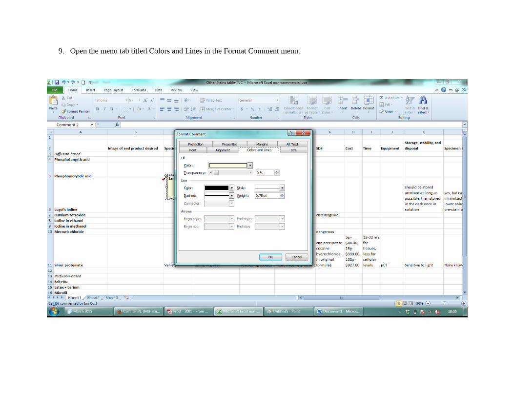
9. Open the menu tab titled Colors and Lines in the Format Comment menu.

10. Under Color and Lines, open the drop menu next to Color and open the last option, Fill Effects.

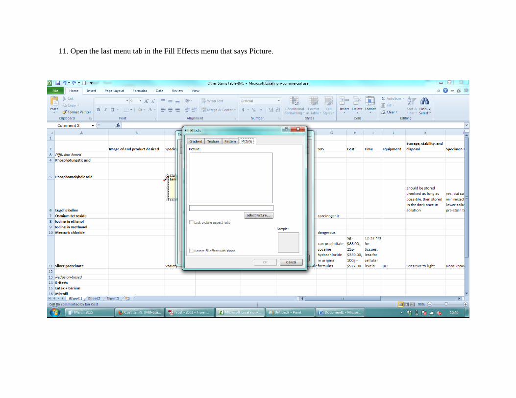
11. Open the last menu tab in the Fill Effects menu that says Picture.

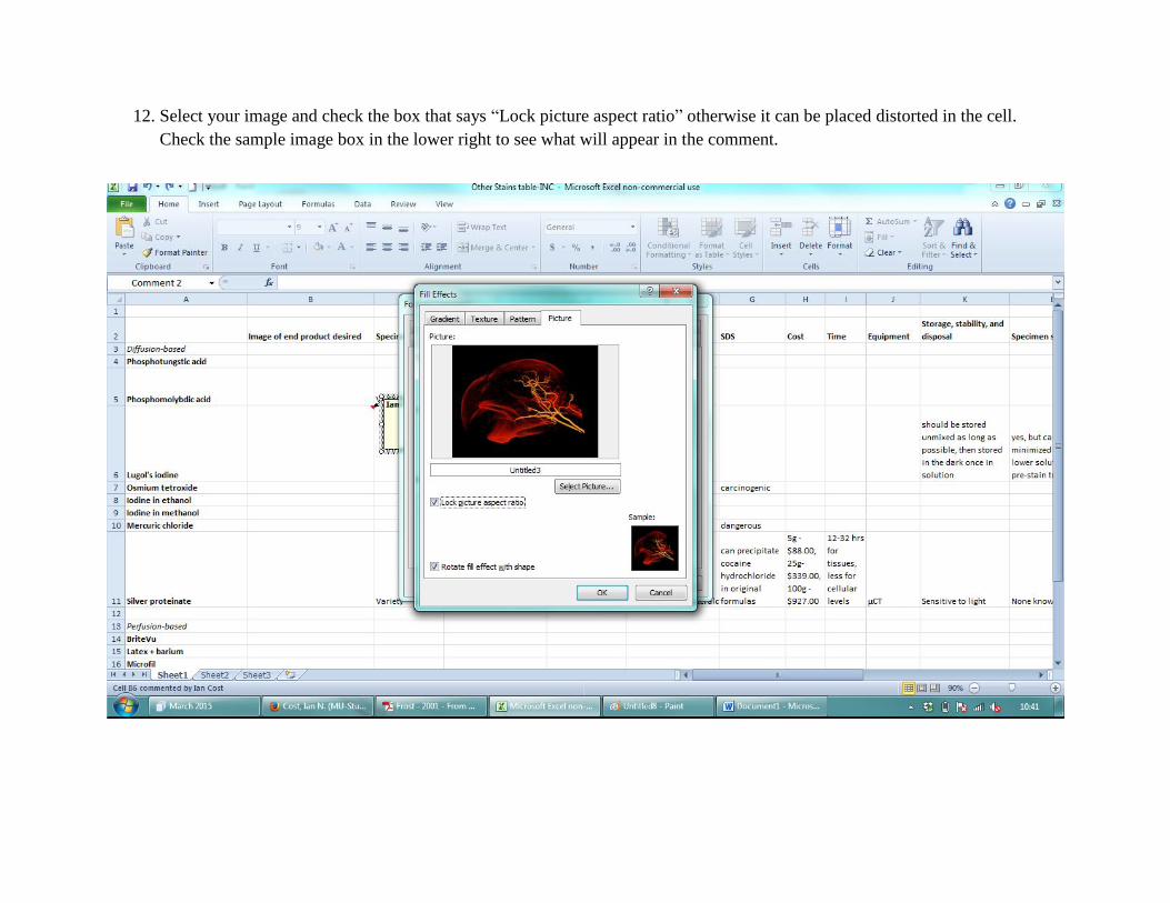
12. Select your image and check the box that says “Lock picture aspect ratio” otherwise it can be placed distorted in the cell.

Check the sample image box in the lower right to see what will appear in the comment.

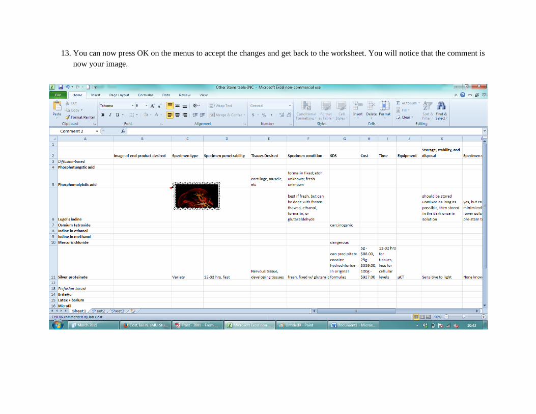
13. You can now press OK on the menus to accept the changes and get back to the worksheet. You will notice that the comment is

now your image.

14. Right click in the cell with your comment and highlight Show/Hide Comments. Click on this to permanently show the

comment you just created.

15. The final step is moving your comment into the cell. You can resize the comment as necessary like you can with a floating

image. If needed, we can change the cell size to accommodate the comment or vice versa.

16. The final product without the grey border looks more natural than a floating image but is still adjustable despite being tied to

the cell that the comment was generated for. After saving the sheet upload to Dropbox and the next person can continue

working!