Select = left click

Click = left click

Use mouse to select cells = ◦ press left mouse button at top of range of cells

◦ while holding down left mouse button drag mouse until all cells desired are highlighted

◦ Release left mouse button

Works in all versions of Excel:

Change Programs: Alt + Tab

Copy: Ctrl + C

Paste : Ctrl + V

Cut: Ctrl + X

Save: Ctrl + S

Undo: Ctrl + Z

On most of Excels menu items you will see the shortcut key associated with it. To see a complete list push F1 and type "Shortcut Keys".

Highlight entire sheet.

Double click on the line between two rows or between two columns.

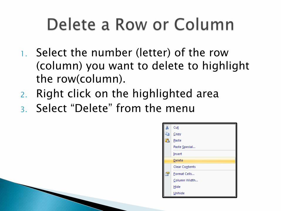
1. Select the number (letter) of the row (column) you want to delete to highlight the row(column).

2. Right click on the highlighted area

3. Select “Delete” from the menu

Select the letter of the row directly under the location you want to insert the new row.

Right click on the highlighted area.

Select “Insert” from the menu.

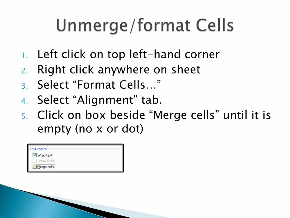
1. Left click on top left-hand corner

2. Right click anywhere on sheet

3. Select “Format Cells…”

4. Select “Alignment” tab.

5. Click on box beside “Merge cells” until it is empty (no x or dot)

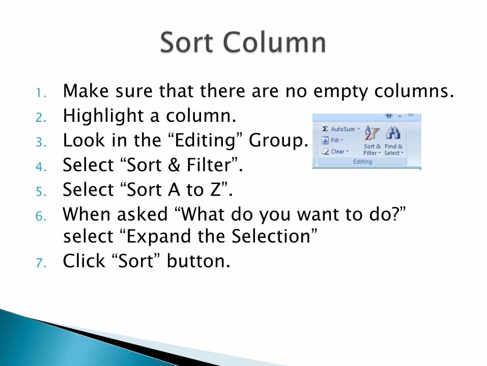
1. Make sure that there are no empty columns.

2. Highlight a column.

3. Look in the “Editing” Group.

4. Select “Sort & Filter”.

5. Select “Sort A to Z”.

6. When asked “What do you want to do?” select “Expand the Selection”

7. Click “Sort” button.

Select area to freeze:◦ Freeze Rows: Click the cell directly under the rows you want

to freeze in Column A◦ Freeze Columns: Click on cell directly to the right of the

columns you want to freeze in row 1◦ Freeze Rows and Columns: Click on the cell directly under

the rows and to the right of the columns you want to freeze Select “Freeze Panes”

◦ Excel 2007: Select “View” tab Select “Freeze Panes” Select “Freeze Panes” (yes again)

◦ Excel 97-2003: Select “Windows” menu from toolbar Select “Freeze Panes”

Find the number of kids with a certain characteristic (Counta from above) and place in a destination cell

Find the total number of kids you are counting (for example, Counta the PIDNumber) and place in a separate destination cell

Select a third destination cell Click formula bar Type “=” Select first destination cell (the number of kids with a

characteristic) Type “/” Select second destination cell It should look something like “=A20/B20”

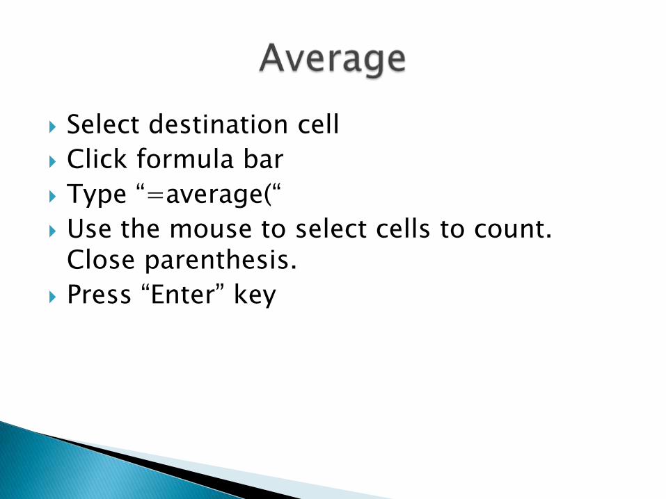
Select destination cell

Click formula bar

Type “=average(“

Use the mouse to select cells to count. Close parenthesis.

Press “Enter” key

Countif(range, “High”)

Select destination cell

Click formula bar

Type “=countif(”

Use the mouse to select the cells to count.

Type “, “High”) “

Press “Enter” key

Pivot Tables

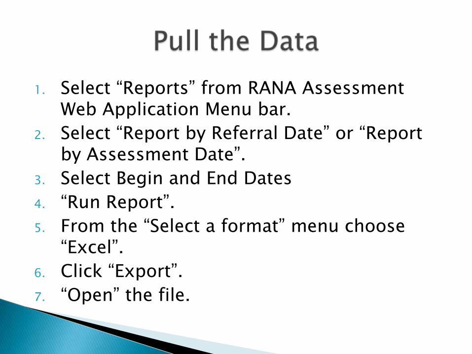
1. Select “Reports” from RANA Assessment Web Application Menu bar.

2. Select “Report by Referral Date” or “Report by Assessment Date”.

3. Select Begin and End Dates

4. “Run Report”.

5. From the “Select a format” menu choose “Excel”.

6. Click “Export”.

7. “Open” the file.

1. Remove the first 4 rows.

2. Unmerge all the cells.

3. Delete empty columns (column K).

Select one cell in the middle of the table

Select the “Insert” tab. From the “Tables” group select

the “PivotTable” menu option. “Select a table or range” should

be already filled with the table. “Choose where you want the

PivotTable report to be placed” should be “New Workbook”

Click “OK”

A new sheet will open for the pivot table.

In the “Drop Page Fields Here” section drag and drop “Status” from the “PivotTable Field List”.

This creates a dropdown box. Click to down arrow to the right of “(All)”. From this menu select “Complete”. Click “OK”.

Next drag the “Gender” field from the “PivotTable Field List”

From the “PivotTable Field List” drag and drop “Gender” into the “Drop Column Fields Here” area.

From the “PivotTable Field List” drag and drop “Risk Level” into the “Drop Row Fields Here” area.

From “PivotTable Field List” drag and drop “PIDNumber” into the “Drop Data Items Here” field

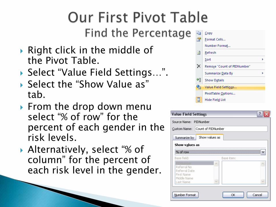
Right click in the middle of the Pivot Table.

Select “Value Field Settings…”.

Select the “Show Value as” tab.

From the drop down menu select “% of row” for the percent of each gender in the risk levels.

Alternatively, select “% of column” for the percent of each risk level in the gender.