exchange rate determination and forecasting: can the...

Hindawi Publishing CorporationISRN EconomicsVolume 2013, Article ID 724259, 12 pageshttp://dx.doi.org/10.1155/2013/724259

Research ArticleExchange Rate Determination and Forecasting:Can the Microstructure Approach Rescue Us fromthe Exchange Rate Disparity?

Guangfeng Zhang,1 Qiong Zhang,2 and Muhammad Tariq Majeed3

1 GREQAM, School of Economics, Aix-Marseille University, Marseille 13236, France2 School of Public Administration, Sichuan University, Chengdu 610000, China3 School of Economics, Quaid-i-Azam University, Islamabad 45320, Pakistan

Correspondence should be addressed to Guangfeng Zhang; [email protected]

Received 21 August 2013; Accepted 1 December 2013

Academic Editors: M. E. Kandil and A. Rodriguez-Alvarez

Copyright © 2013 Guangfeng Zhang et al. This is an open access article distributed under the Creative Commons AttributionLicense, which permits unrestricted use, distribution, and reproduction in any medium, provided the original work is properlycited.

Using two measures of private information and high-frequency transaction data from the leading interdealer electronic brokingsystem Reuters D2000-2, we examine the association between exchange rate return and contemporaneous order flow and thepredictability power of lagged order flow on the future exchange rate return. Our empirical analysis demonstrates that at highfrequency (5, 10, 15, 20, 25, and 30min) there exists strong positive association between exchange rate returns and contemporaneousorder flow. However, the results indicate weak predictability of order flow on the future exchange rate return.

1. Introduction

In exchange rate economics one conventional common senseabout exchange rates is that exchange rates follow a randomwalk process for frequencies less than annual, such as daily,weekly, or even monthly. However, exchange rates showsome trend, cyclicality, or general history dependence atlower frequencies. In contrast to macroeconomic fundamen-tal analysis at lower frequencies, studies on microstructureapproaches to exchange rates focus on the movements inexchange rates at high frequency. In particular, microstruc-ture approaches emphasize how exchange rates respond toorder flow, which measures the net transaction pressurebetween buy and sell forces in the actual FX market.

The theoretical frameworks for microstructureapproaches to exchange rates have been sequentiallybuilt by Lyons [1] and Evans and Lyons [2]. In particular,the portfolio-shift model proposed by Evans and Lyons [2]is initially set up in a customer-dealer trading environmentto show how order flow impacts exchange rates. Evans andLyons apply the trading model to daily data obtained fromthe customer-dealer transaction platform Reuters D2000-1

to examine the exchange rate Deutsche mark/US dollarand Japanese yen/US dollar over May 1 to August 31, 1996.As a result, Evans and Lyons find that order flow can be agood series to determine the exchange rate movement atdaily frequency. Similarly, empirical studies have applied thistheoretical framework to various high-frequency data fromdiverse interdealer trading platforms. Killeen et al. [3] studythe daily exchange rate German mark/French franc tradedon the electronic broking system (EBS) in 1998. Hau et al.[4] study EBS data over 1998 to 1999 on the exchange rateGerman mark against US dollar. Berger et al. [5] study theintraday EBS data on the exchange rate US dollar/Japaneseyen and Euro/US dollar spanning over January 1999 toFebruary 2004. Ito and Hashimoto [6] study the intradayEBS data on the exchange rate US dollar/Japanese yen overJanuary 4, 1998 to October 31, 2003 and Euro/US dollarover January 3, 1999 to October 31, 2003. Relevant studiesalso have examined the data from central banks. Rime [7]applies weekly data from Norges Bank for the exchangerate Deutsche mark/US dollar, British pound/US dollar,and Swiss franc/US dollar over July 1995 to September1999. Payne [8] employs the tick-by-tick real-time foreign

2 ISRN Economics

exchange trading data of Deutsche mark/US dollar from theinterdealer FX trading system Reuters D2000-2. Overall,these studies consistently confirm a significant positiveassociation between exchange rates and the correspondingcontemporaneous order flow.

We aim to revisit the association between exchange ratesand contemporaneous order flow and the predictability ofthe lagged order flow on the future exchange rate. Our studyuses the intraday high-frequency transaction data from oneof the leading interdealer electronic broking systems, ReutersD2000-2.We implement the empirical analysis via two differ-ent measures of order flow. Our analysis demonstrates thatat high frequency (5, 10, 15, 20, 25, and 30min) there existsa strong positive association between exchange rate returnand contemporaneous order flow. However, our empiricalstudy shows weak predictability of order flow on the futureexchange rate return.We also investigate the feedback tradingin the FX market, but in our case this common theoreticalhypothesis is rejected in our empirical analysis.

Comparing with relevant researches, our study is distinctfrom others in terms of the approach to measure order flow,the approach to implement the contemporaneous associationand future prediction, and our particular data set. First, weuse two different measurements of order flow to identifythe impact of order flow on the contemporaneous exchangerate and the prediction of order flow on the future exchangerate. Related researches usually adopt the number of the nettransactions (number of buyer-initiated trade minus numberof seller-initiated trade) to proxy the absolute value of orderflow, which is originally defined as the net value betweenthe buyer-initiated trade and seller-initiated trade. We usethe net transaction values in our empirical study though thenumber of transactions is adopted in relevant studies. Inparticular, in our empirical analysis, we also use the ratioof the absolute order flow to the trade flow to proxy orderflow. Second, we examine the possible endogeneity of thecontemporaneous order flow from the feedback trading andpossible nonlinearity involved in the association. Third, weseparately examine the contemporaneous determination ofthe exchange rate and the prediction power of the laggedorder flow on the future exchange rate return. In the analysisof prediction, we identify the relative weak predictability ofthe history order flowon the future return, theweak historicaldependence of order flow, and the high market efficiency inthe actual FX market. Finally, it is worth mentioning thatwe use the transaction data for the exchange rate Deutschemark/US dollar from one of the leading brokered interdealertrading system, Reuters D2000-2. Relevant researches haveextensively examined the transaction data from customer-dealer platform, central banks, direct interdealer transactionplatformReutersD2000-1, and broker interdealer transactionplatform EBS. As we discussed in the survey section thatthe data from different source usually represent differentcharacteristics of the trading agents in the FX market, whichmakes the association using the data from this differentsource worth revisiting.

The structure of this paper is as follows. Section 2 brieflyintroduces the theoretical issue about the association betweenexchange rates and order flow. Section 3 describes the data

and constructs the series used in our empirical analysis.Section 4 introduces themethodology arrangements adoptedin our empirical study. Section 5 reports the results of ourempirical studies. Section 6 concludes this paper.

2. Theoretical Issue

The theoretical models proposed by Lyons [1] and Evansand Lyons [2] are designed to fit the structure of the actualforeign exchange trading process.The twomodels are termedas, respectively, hot-potato trading and portfolio-shiftmodel.Particularly, Evans and Lyons [2] frame the real market-markers’ behaviours in the FX market. Their model capturesthe important aspects of exchange rate determinations causedby the actual foreign exchange transactions between themarket participants. Formore details about themodel details,see Lyons [1] and Evans and Lyons [2]. We summarize therelationship between the exchange rate return Δ𝑝

𝑡and the

order flow 𝑥𝑡in the specification as follows:

Δ𝑝𝑡= 𝛼 + 𝛽𝑥

𝑡+ 𝜀𝑡. (1)

As the theoretical model suggested, the positive net transac-tion pressure between buying and selling increases the valueof the exchange rate which is defined as the domestic price ofthe foreign currency.The coefficient𝛽 on order flow𝑥

𝑡should

take positive value. On the contrary, the negative net transac-tion pressure decreases the value of the exchange rate. As tothe association between exchange rate return Δ𝑝

𝑡and order

flow 𝑥𝑡, practical studies are concerned with the causation

relationship between these two series. Representative studies,such as those of Killeen et al. [3] and Payne [8], use the VARstructure and Johansen cointegration procedure to examinethe long-run association involved. They demonstrate a long-run cointegration relationship between exchange rates andorder flow, but a single direction of causality from orderflow to the exchange rate return. According to the theoreticalframework of Evans and Lyons [2], our empirical studyexamines the impact of order flow on the contemporaneousexchange rate return and the predictability of order flow onthe future exchange rate return.

3. Data Description and Construction

Our empirical analysis uses the real transaction data for theexchange rate Deutsche mark/US dollar over October 6 toOctober 10, 1997. The data comes from one of the leadingelectronic FX transaction platforms, Reuters D2000-2, whichis updated to D3000-2 now. The original dataset containstwo data files. One dataset records the real-time quotes forthe exchange rate Deutsche mark against US dollar, whichincludes the time stamp, the best bid price, and the best askprice at a particular time. The other dataset records the real-time trade, which includes the time stamp, the trade quantity,the trade direction, and the trade price. The vast majority oftransactions on Deutsche mark/US dollar take place between6 am and 6 pm,Monday to Friday although foreign exchangetransaction takes place on the Reuters system D2000-2 24hours a day and 7 days a week. The empirical analyses in

ISRN Economics 3

1.732

1.736

1.740

1.744

1.748

1.752

1.756

1.760

1.764

100 200 300 400 500 600

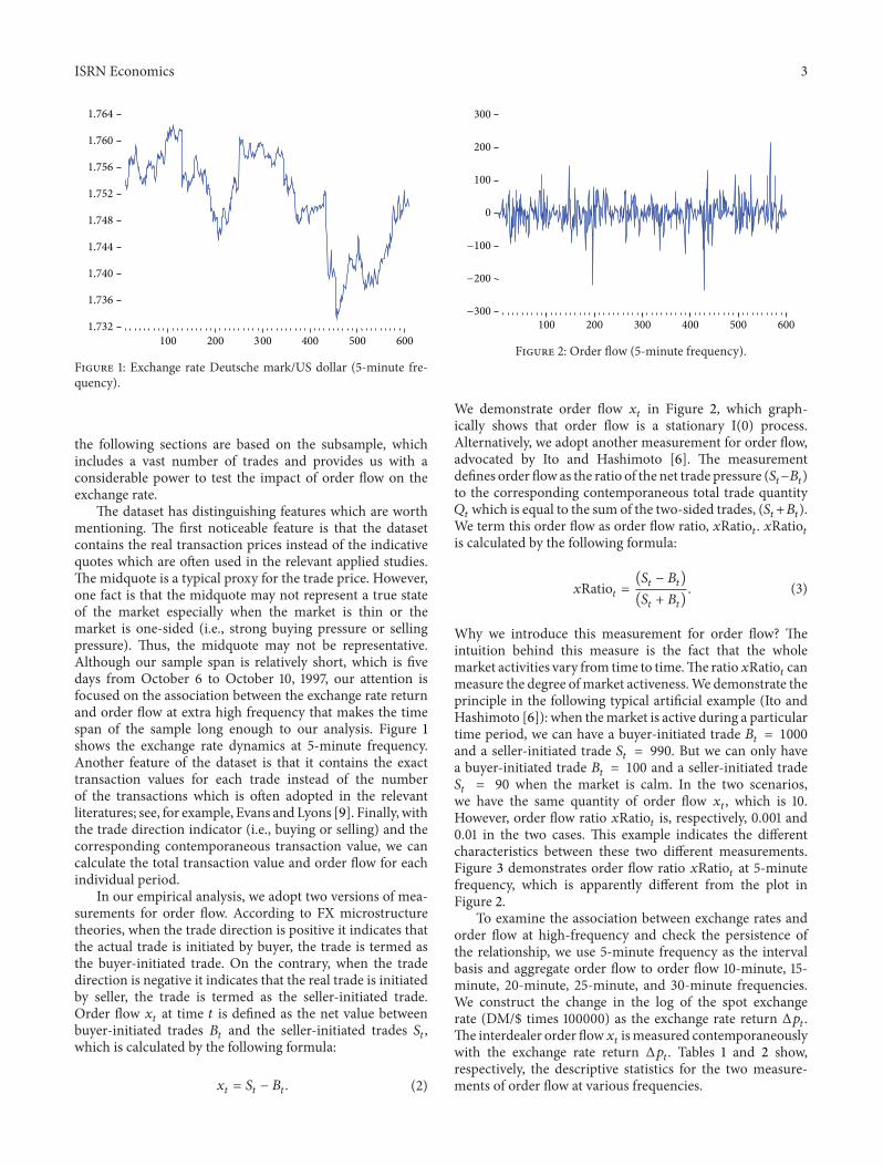
Figure 1: Exchange rate Deutsche mark/US dollar (5-minute fre-quency).

the following sections are based on the subsample, whichincludes a vast number of trades and provides us with aconsiderable power to test the impact of order flow on theexchange rate.

The dataset has distinguishing features which are worthmentioning. The first noticeable feature is that the datasetcontains the real transaction prices instead of the indicativequotes which are often used in the relevant applied studies.The midquote is a typical proxy for the trade price. However,one fact is that the midquote may not represent a true stateof the market especially when the market is thin or themarket is one-sided (i.e., strong buying pressure or sellingpressure). Thus, the midquote may not be representative.Although our sample span is relatively short, which is fivedays from October 6 to October 10, 1997, our attention isfocused on the association between the exchange rate returnand order flow at extra high frequency that makes the timespan of the sample long enough to our analysis. Figure 1shows the exchange rate dynamics at 5-minute frequency.Another feature of the dataset is that it contains the exacttransaction values for each trade instead of the numberof the transactions which is often adopted in the relevantliteratures; see, for example, Evans and Lyons [9]. Finally, withthe trade direction indicator (i.e., buying or selling) and thecorresponding contemporaneous transaction value, we cancalculate the total transaction value and order flow for eachindividual period.

In our empirical analysis, we adopt two versions of mea-surements for order flow. According to FX microstructuretheories, when the trade direction is positive it indicates thatthe actual trade is initiated by buyer, the trade is termed asthe buyer-initiated trade. On the contrary, when the tradedirection is negative it indicates that the real trade is initiatedby seller, the trade is termed as the seller-initiated trade.Order flow 𝑥

𝑡at time 𝑡 is defined as the net value between

buyer-initiated trades 𝐵𝑡and the seller-initiated trades 𝑆

𝑡,

which is calculated by the following formula:

𝑥𝑡= 𝑆𝑡− 𝐵𝑡. (2)

0

100

200

300

100 200 300 400 500 600−300

−200

−100

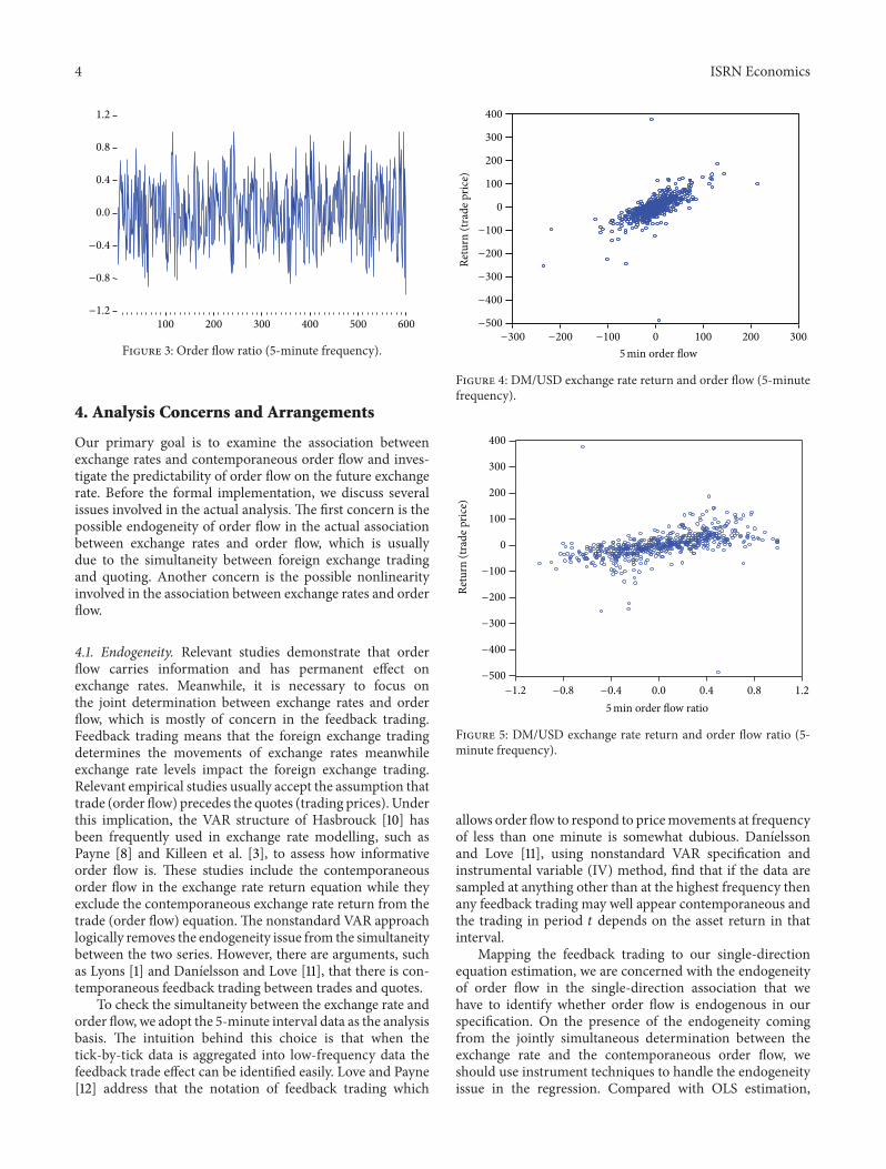
Figure 2: Order flow (5-minute frequency).

We demonstrate order flow 𝑥𝑡in Figure 2, which graph-

ically shows that order flow is a stationary I(0) process.Alternatively, we adopt another measurement for order flow,advocated by Ito and Hashimoto [6]. The measurementdefines order flow as the ratio of the net trade pressure (𝑆

𝑡−𝐵𝑡)

to the corresponding contemporaneous total trade quantity𝑄𝑡which is equal to the sum of the two-sided trades, (𝑆

𝑡+𝐵𝑡).

We term this order flow as order flow ratio, 𝑥Ratio𝑡. 𝑥Ratio

𝑡

is calculated by the following formula:

𝑥Ratio𝑡=(𝑆𝑡− 𝐵𝑡)

(𝑆𝑡+ 𝐵𝑡). (3)

Why we introduce this measurement for order flow? Theintuition behind this measure is the fact that the wholemarket activities vary from time to time.The ratio𝑥Ratio

𝑡can

measure the degree ofmarket activeness.We demonstrate theprinciple in the following typical artificial example (Ito andHashimoto [6]): when themarket is active during a particulartime period, we can have a buyer-initiated trade 𝐵

𝑡= 1000

and a seller-initiated trade 𝑆𝑡= 990. But we can only have

a buyer-initiated trade 𝐵𝑡= 100 and a seller-initiated trade

𝑆𝑡= 90 when the market is calm. In the two scenarios,

we have the same quantity of order flow 𝑥𝑡, which is 10.

However, order flow ratio 𝑥Ratio𝑡is, respectively, 0.001 and

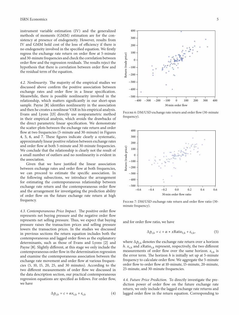
0.01 in the two cases. This example indicates the differentcharacteristics between these two different measurements.Figure 3 demonstrates order flow ratio 𝑥Ratio

𝑡at 5-minute

frequency, which is apparently different from the plot inFigure 2.

To examine the association between exchange rates andorder flow at high-frequency and check the persistence ofthe relationship, we use 5-minute frequency as the intervalbasis and aggregate order flow to order flow 10-minute, 15-minute, 20-minute, 25-minute, and 30-minute frequencies.We construct the change in the log of the spot exchangerate (DM/$ times 100000) as the exchange rate return Δ𝑝

𝑡.

The interdealer order flow𝑥𝑡ismeasured contemporaneously

with the exchange rate return Δ𝑝𝑡. Tables 1 and 2 show,

respectively, the descriptive statistics for the two measure-ments of order flow at various frequencies.

4 ISRN Economics

0.0

0.4

0.8

1.2

100 200 300 400 500 600−1.2

−0.8

−0.4

Figure 3: Order flow ratio (5-minute frequency).

4. Analysis Concerns and Arrangements

Our primary goal is to examine the association betweenexchange rates and contemporaneous order flow and inves-tigate the predictability of order flow on the future exchangerate. Before the formal implementation, we discuss severalissues involved in the actual analysis. The first concern is thepossible endogeneity of order flow in the actual associationbetween exchange rates and order flow, which is usuallydue to the simultaneity between foreign exchange tradingand quoting. Another concern is the possible nonlinearityinvolved in the association between exchange rates and orderflow.

4.1. Endogeneity. Relevant studies demonstrate that orderflow carries information and has permanent effect onexchange rates. Meanwhile, it is necessary to focus onthe joint determination between exchange rates and orderflow, which is mostly of concern in the feedback trading.Feedback trading means that the foreign exchange tradingdetermines the movements of exchange rates meanwhileexchange rate levels impact the foreign exchange trading.Relevant empirical studies usually accept the assumption thattrade (order flow) precedes the quotes (trading prices). Underthis implication, the VAR structure of Hasbrouck [10] hasbeen frequently used in exchange rate modelling, such asPayne [8] and Killeen et al. [3], to assess how informativeorder flow is. These studies include the contemporaneousorder flow in the exchange rate return equation while theyexclude the contemporaneous exchange rate return from thetrade (order flow) equation. The nonstandard VAR approachlogically removes the endogeneity issue from the simultaneitybetween the two series. However, there are arguments, suchas Lyons [1] and Danı́elsson and Love [11], that there is con-temporaneous feedback trading between trades and quotes.

To check the simultaneity between the exchange rate andorder flow, we adopt the 5-minute interval data as the analysisbasis. The intuition behind this choice is that when thetick-by-tick data is aggregated into low-frequency data thefeedback trade effect can be identified easily. Love and Payne[12] address that the notation of feedback trading which

−500

−400

−300

−200

−100

0

100

200

300

400

−300 −200 −100 0 100 200 300

Retu

rn (t

rade

pric

e)

5min order flow

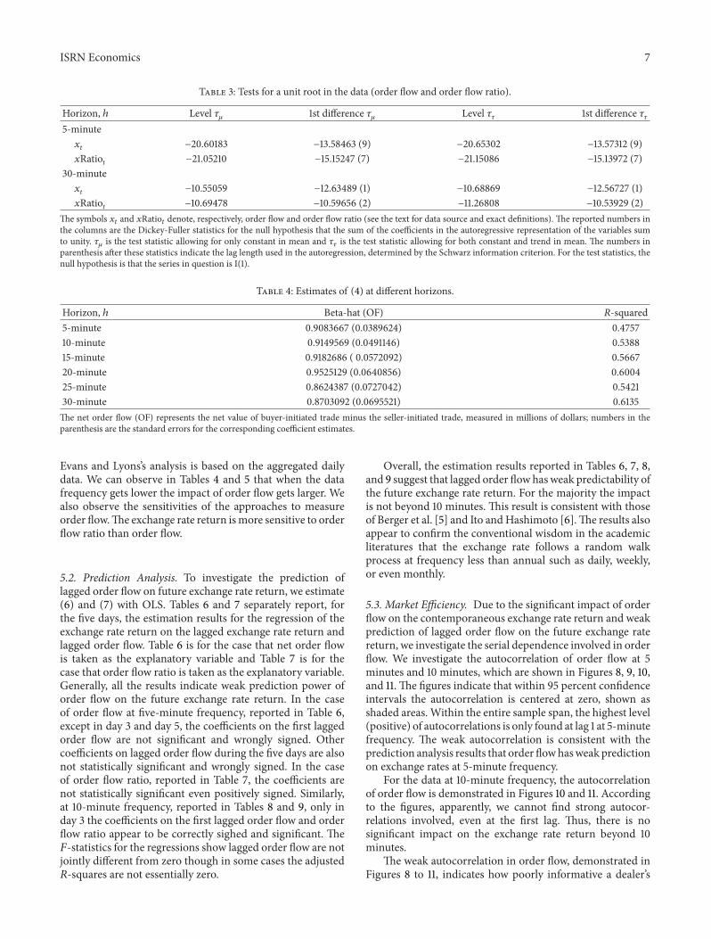
Figure 4: DM/USD exchange rate return and order flow (5-minutefrequency).

−500

−400

−300

−200

−100

0

100

200

300

400

Retu

rn (t

rade

pric

e)

−1.2 −0.8 −0.4 0.0 0.4 0.8 1.2

5min order flow ratio

Figure 5: DM/USD exchange rate return and order flow ratio (5-minute frequency).

allows order flow to respond to pricemovements at frequencyof less than one minute is somewhat dubious. Danı́elssonand Love [11], using nonstandard VAR specification andinstrumental variable (IV) method, find that if the data aresampled at anything other than at the highest frequency thenany feedback trading may well appear contemporaneous andthe trading in period 𝑡 depends on the asset return in thatinterval.

Mapping the feedback trading to our single-directionequation estimation, we are concerned with the endogeneityof order flow in the single-direction association that wehave to identify whether order flow is endogenous in ourspecification. On the presence of the endogeneity comingfrom the jointly simultaneous determination between theexchange rate and the contemporaneous order flow, weshould use instrument techniques to handle the endogeneityissue in the regression. Compared with OLS estimation,

ISRN Economics 5

instrument variable estimation (IV) and the generalizedmethods of moments (GMM) estimation are for the con-sistency at presence of endogeneity. However, results fromIV and GMM hold cost of the loss of efficiency if there isno endogeneity involved in the specified equation. We firstlyregress the exchange rate return on order flow at 5-minuteand 30-minute frequencies and check the correlation betweenorder flow and the regression residuals. The results reject thehypothesis that there is correlation between order flow andthe residual term of the equation.

4.2. Nonlinearity. The majority of the empirical studies wediscussed above confirm the positive association betweenexchange rates and order flow in a linear specification.Meanwhile, there is possible nonlinearity involved in therelationship, which matters significantly in our short-spansample. Payne [8] identifies nonlinearity in the associationand then he creates a nonlinear VAR in his empirical analysis.Evans and Lyons [13] directly use nonparametric methodin their empirical analysis, which avoids the drawbacks ofthe direct parametric linear specification. We demonstratethe scatter-plots between the exchange rate return and orderflow at two frequencies (5-minute and 30-minute) in Figures4, 5, 6, and 7. These figures indicate clearly a systematic,approximately linear positive relation between exchange ratesand order flow at both 5-minute and 30-minute frequencies.We conclude that the relationship is clearly not the result ofa small number of outliers and no nonlinearity is evident inthe association.

Given that we have justified the linear associationbetween exchange rates and order flow at both frequencies,we can proceed to estimate the specific association. Inthe following subsections, we introduce the arrangementfor estimating the contemporaneous relationship betweenexchange rate return and the contemporaneous order flowand the arrangement for investigating the prediction abilityof order flow on the future exchange rate return at highfrequency.

4.3. Contemporaneous Price Impact. The positive order flowrepresents net buying pressure and the negative order flowrepresents net selling pressure. Thus, we expect that buyingpressure raises the transaction prices and selling pressurelowers the transaction prices. In the studies we discussedin previous sections the return equation includes both thecontemporaneous and lagged order flows as the explanatorydeterminants, such as those of Evans and Lyons [2] andPayne [8]. Slightly different, at this stage we only include thecontemporaneous order flow in the determination regressionand examine the contemporaneous association between theexchange rate movement and order flow at various frequen-cies (5, 10, 15, 20, 25, and 30 minutes). According to thetwo different measurements of order flow we discussed inthe data description section, our practical contemporaneousregression equations are specified as follows. For order flow,we have

Δ𝑝𝑡,ℎ= 𝑐 + 𝛼𝑥

𝑡,ℎ+ 𝜀𝑡,ℎ

(4)

−500

−400

−300

−200

−100

0

100

200

300

400

−300−400 −200 −100 0 100 200 300 400

Retu

rn (t

rade

pric

e)

30min order flow

Figure 6: DM/USD exchange rate return and order flow (30-minutefrequency).

−0.6 −0.4 −0.2 0.0 0.2 0.4 0.6

−500

−400

−300

−200

−100

0

100

200

300

400

Retu

rn (t

rade

pric

e)

30min order flow ratio

Figure 7: DM/USD exchange rate return and order flow ratio (30-minute frequency).

and for order flow ratio, we have

Δ𝑝𝑡,ℎ= 𝑐 + 𝛼 ∗ 𝑥Ratio

𝑡,ℎ+ 𝜀𝑡,ℎ, (5)

where Δ𝑝𝑡,ℎ

denotes the exchange rate return over a horizonℎ. 𝑥𝑡,ℎ

and 𝑥Ratio𝑡,ℎ

represent, respectively, the two differentmeasurements of order flow over the same horizon. 𝜀

𝑡,ℎis

the error term. The horizon ℎ is initially set up at 5-minutefrequency to calculate order flow. We aggregate the 5-minuteorder flow to order flow at 10-minute, 15-minute, 20-minute,25-minute, and 30-minute frequencies.

4.4. Future Price Prediction. To directly investigate the pre-diction power of order flow on the future exchange ratereturn, we only include the lagged exchange rate returns andlagged order flow in the return equation. Corresponding to

6 ISRN Economics

Table 1: Order flow descriptive statistics at different horizons.

5 minutes 10 minutes 15 minutes 20 minutes 25 minutes 30 minutesMean 0.881667 1.763333 2.645000 3.526667 4.408333 5.290000Median 1.500000 5.000000 8.000000 4.000000 1.000000 6.000000Maximum 215.0000 269.0000 356.0000 410.0000 283.0000 324.0000Minimum −234.0000 −197.0000 −321.0000 −279.0000 −345.0000 −366.0000Std. dev. 39.64055 58.94865 76.67211 90.37102 102.3269 115.9329This table reports some summary statistics for order flow, measured in millions of dollars, at 5-minute frequency, and aggregated to 10-minute, 15-minute, 20-minute, 25-minute, and 30-minute frequencies.

Table 2: Order flow ratio descriptive statistics at different horizons.

5 minutes 10 minutes 15 minutes 20 minutes 25 minutes 30 minutesMean 0.031845 0.027866 0.026526 0.029278 0.025767 0.020082Median 0.032796 0.043438 0.043140 0.015080 0.001379 0.023331Maximum 1.000000 0.736842 0.709924 0.684211 0.531429 0.435780Minimum −1.000000 −0.729167 −0.725191 −0.531469 −0.517647 −0.428571Std. dev. 0.392208 0.304738 0.270706 0.236041 0.219407 0.195233This table reports some summary statistics for order flow ratiomeasured at 5-minute frequency and aggregated to 10-minute, 15-minute, 20-minute, 25-minute,and 30-minute frequencies.

the two contemporaneous determination equations above, wespecify the two prediction associations as follows:

Δ𝑝𝑡= 𝛽0+

𝑚

∑

𝑖=1

𝛾𝑖Δ𝑝𝑡−𝑖+

𝑚

∑

𝑖

𝛿𝑖𝑥𝑡−𝑖+ 𝜀𝑡, (6)

Δ𝑝𝑡= 𝛽0+

𝑚

∑

𝑖=1

𝛾𝑖Δ𝑝𝑡−𝑖+

𝑚

∑

𝑖

𝛿𝑖𝑥Ratio

𝑡−𝑖+ 𝜀𝑡, (7)

where Δ𝑝𝑡denotes the exchange rate return from period 𝑡−1

to 𝑡. 𝑥𝑡−𝑖

is the lagged order flow. We regress the exchangerate return on the lagged order flow and lagged exchange ratereturn at 5 minutes and 10 minutes, respectively. We choose5 as the maximum lag 𝑚 for both the exchange rate returnand order flow. With the maximum lag 5, we aim to testwhether the predictability of order flow can be ahead of half-hour when the data is measured at 5-minute frequency andone-hour when the data is measured at 10-minute frequency.Considering the discontinuity of the data (we only focus onperiod from 06:00 am to 06:00 pm in our contemporaneousanalysis), we separately examine the prediction power oforder flow in the Granger-causality regressions, based on thedata from the five different days.

5. Empirical Data Analysis

During the test whether order flow is endogenous in the con-temporaneous regression, we fail to accept the hypothesis thatthe order flow is correlated with the regression residual term.Moreover, this conclusion is valid for the two measurementsof order flow at all the chosen frequencies.Thus, we accept thevalidity of the assumption that trading precedes the quoting.For relevant studies, see those of Evans and Lyons [2], Bergeret al. [5], and Ito and Hashimoto [6].

5.1. Contemporaneous Price Impact. Before the actual esti-mation, we firstly investigate whether the two measurementsof order flow in our study, order flow and order flowratio, are stationary processes. Killeen et al. [3] find a long-run cointegration relation between exchange rate levels andcumulated order flow. In our relative short sample, we expectthat the two measures of order flow are stationary processes,which are shown in Figures 2 and 3. Table 3 reports the unitroot test results for the two measurements of order flow at5-minute and 30-minute frequencies. The tests confirm thatorder flow and order flow ratio are consistently I(0) series at10-minute, 15-minute, 20-minute, and 25-minute frequencies.

According to (4) and (5), we use OLS to implement theestimation of the contemporaneous association. Tables 4 and5 report the estimation results for the impact of order flowon the contemporaneous exchange rate return. For the twomeasurements of order flow, the results suggest that all thecoefficient estimates are statistically significant and correctlysigned at all frequencies. The magnitudes of the coefficientson order flow imply that the contemporaneous impact oforder flow is significant. The determination coefficient 𝑅-squares ranges from 47 percent to 61 percent for the case oforder flow and varies from 26 percent to 52 percent for thecase of order flow ratio. These results are consistent with thestudy of Evans and Lyons [9]. We also separately regress theexchange rate return on order flow for the five days of oursample and the estimates are significantly close to those wereport here.

Our coefficient estimates reported in Tables 4 and 5 areconsistent with our theoretical hypothesis. Meanwhile, theyare different in magnitude from the estimates of Evans andLyons [9].We think one possible reason could be because ourestimate is concerned the association between the exchangerate return with order flow at a higher frequency, that is, 5-minute and 10-minute frequencies, and so forth. However,

ISRN Economics 7

Table 3: Tests for a unit root in the data (order flow and order flow ratio).

Horizon, ℎ Level 𝜏𝜇

1st difference 𝜏𝜇

Level 𝜏𝜏

1st difference 𝜏𝜏

5-minute𝑥𝑡

−20.60183 −13.58463 (9) −20.65302 −13.57312 (9)𝑥Ratio

𝑡−21.05210 −15.15247 (7) −21.15086 −15.13972 (7)

30-minute𝑥𝑡

−10.55059 −12.63489 (1) −10.68869 −12.56727 (1)𝑥Ratio

𝑡−10.69478 −10.59656 (2) −11.26808 −10.53929 (2)

The symbols 𝑥𝑡and 𝑥Ratio

𝑡denote, respectively, order flow and order flow ratio (see the text for data source and exact definitions). The reported numbers in

the columns are the Dickey-Fuller statistics for the null hypothesis that the sum of the coefficients in the autoregressive representation of the variables sumto unity. 𝜏

𝜇is the test statistic allowing for only constant in mean and 𝜏

𝜏is the test statistic allowing for both constant and trend in mean. The numbers in

parenthesis after these statistics indicate the lag length used in the autoregression, determined by the Schwarz information criterion. For the test statistics, thenull hypothesis is that the series in question is I(1).

Table 4: Estimates of (4) at different horizons.

Horizon, ℎ Beta-hat (OF) 𝑅-squared5-minute 0.9083667 (0.0389624) 0.475710-minute 0.9149569 (0.0491146) 0.538815-minute 0.9182686 ( 0.0572092) 0.566720-minute 0.9525129 (0.0640856) 0.600425-minute 0.8624387 (0.0727042) 0.542130-minute 0.8703092 (0.0695521) 0.6135The net order flow (OF) represents the net value of buyer-initiated trade minus the seller-initiated trade, measured in millions of dollars; numbers in theparenthesis are the standard errors for the corresponding coefficient estimates.

Evans and Lyons’s analysis is based on the aggregated dailydata. We can observe in Tables 4 and 5 that when the datafrequency gets lower the impact of order flow gets larger. Wealso observe the sensitivities of the approaches to measureorder flow.The exchange rate return ismore sensitive to orderflow ratio than order flow.

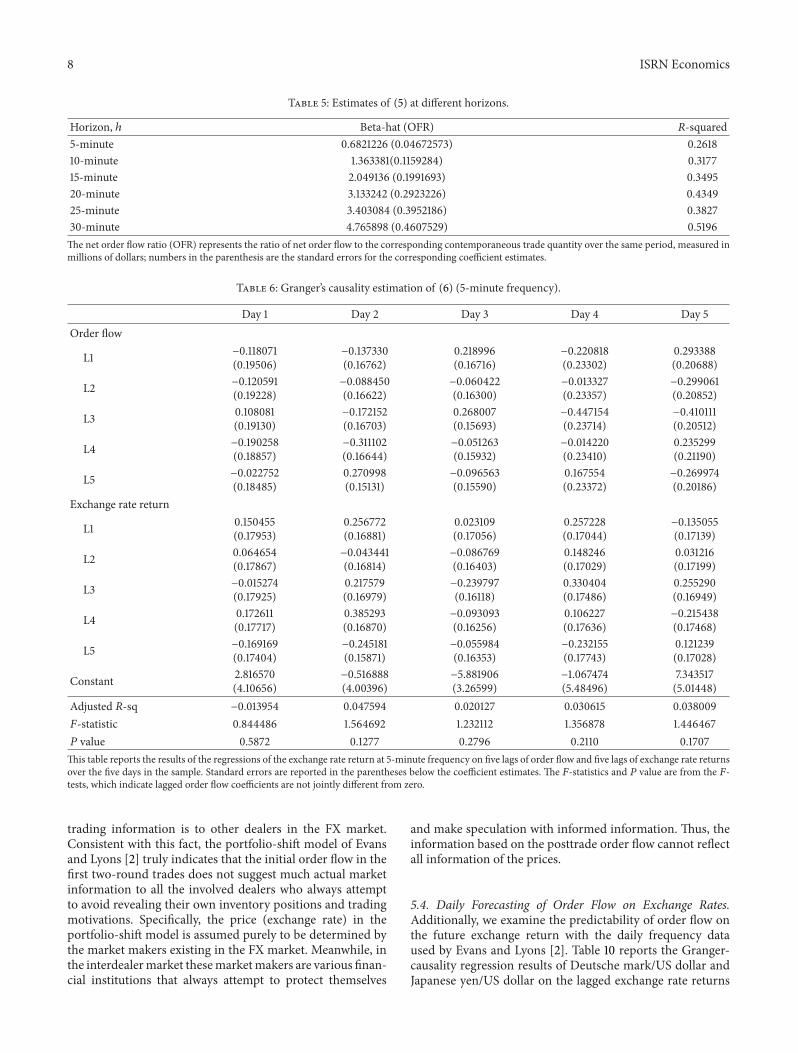
5.2. Prediction Analysis. To investigate the prediction oflagged order flow on future exchange rate return, we estimate(6) and (7) with OLS. Tables 6 and 7 separately report, forthe five days, the estimation results for the regression of theexchange rate return on the lagged exchange rate return andlagged order flow. Table 6 is for the case that net order flowis taken as the explanatory variable and Table 7 is for thecase that order flow ratio is taken as the explanatory variable.Generally, all the results indicate weak prediction power oforder flow on the future exchange rate return. In the caseof order flow at five-minute frequency, reported in Table 6,except in day 3 and day 5, the coefficients on the first laggedorder flow are not significant and wrongly signed. Othercoefficients on lagged order flow during the five days are alsonot statistically significant and wrongly signed. In the caseof order flow ratio, reported in Table 7, the coefficients arenot statistically significant even positively signed. Similarly,at 10-minute frequency, reported in Tables 8 and 9, only inday 3 the coefficients on the first lagged order flow and orderflow ratio appear to be correctly sighed and significant. The𝐹-statistics for the regressions show lagged order flow are notjointly different from zero though in some cases the adjusted𝑅-squares are not essentially zero.

Overall, the estimation results reported in Tables 6, 7, 8,and 9 suggest that lagged order flowhasweak predictability ofthe future exchange rate return. For the majority the impactis not beyond 10 minutes. This result is consistent with thoseof Berger et al. [5] and Ito andHashimoto [6].The results alsoappear to confirm the conventional wisdom in the academicliteratures that the exchange rate follows a random walkprocess at frequency less than annual such as daily, weekly,or even monthly.

5.3. Market Efficiency. Due to the significant impact of orderflow on the contemporaneous exchange rate return and weakprediction of lagged order flow on the future exchange ratereturn, we investigate the serial dependence involved in orderflow. We investigate the autocorrelation of order flow at 5minutes and 10 minutes, which are shown in Figures 8, 9, 10,and 11. The figures indicate that within 95 percent confidenceintervals the autocorrelation is centered at zero, shown asshaded areas.Within the entire sample span, the highest level(positive) of autocorrelations is only found at lag 1 at 5-minutefrequency. The weak autocorrelation is consistent with theprediction analysis results that order flowhasweak predictionon exchange rates at 5-minute frequency.

For the data at 10-minute frequency, the autocorrelationof order flow is demonstrated in Figures 10 and 11. Accordingto the figures, apparently, we cannot find strong autocor-relations involved, even at the first lag. Thus, there is nosignificant impact on the exchange rate return beyond 10minutes.

The weak autocorrelation in order flow, demonstrated inFigures 8 to 11, indicates how poorly informative a dealer’s

8 ISRN Economics

Table 5: Estimates of (5) at different horizons.

Horizon, ℎ Beta-hat (OFR) 𝑅-squared5-minute 0.6821226 (0.04672573) 0.261810-minute 1.363381(0.1159284) 0.317715-minute 2.049136 (0.1991693) 0.349520-minute 3.133242 (0.2923226) 0.434925-minute 3.403084 (0.3952186) 0.382730-minute 4.765898 (0.4607529) 0.5196The net order flow ratio (OFR) represents the ratio of net order flow to the corresponding contemporaneous trade quantity over the same period, measured inmillions of dollars; numbers in the parenthesis are the standard errors for the corresponding coefficient estimates.

Table 6: Granger’s causality estimation of (6) (5-minute frequency).

Day 1 Day 2 Day 3 Day 4 Day 5Order flow

L1 −0.118071(0.19506)

−0.137330(0.16762)

0.218996(0.16716)

−0.220818(0.23302)

0.293388(0.20688)

L2 −0.120591(0.19228)

−0.088450(0.16622)

−0.060422(0.16300)

−0.013327(0.23357)

−0.299061(0.20852)

L3 0.108081(0.19130)

−0.172152(0.16703)

0.268007(0.15693)

−0.447154(0.23714)

−0.410111(0.20512)

L4 −0.190258(0.18857)

−0.311102(0.16644)

−0.051263(0.15932)

−0.014220(0.23410)

0.235299(0.21190)

L5 −0.022752(0.18485)

0.270998(0.15131)

−0.096563(0.15590)

0.167554(0.23372)

−0.269974(0.20186)

Exchange rate return

L1 0.150455(0.17953)

0.256772(0.16881)

0.023109(0.17056)

0.257228(0.17044)

−0.135055(0.17139)

L2 0.064654(0.17867)

−0.043441(0.16814)

−0.086769(0.16403)

0.148246(0.17029)

0.031216(0.17199)

L3 −0.015274(0.17925)

0.217579(0.16979)

−0.239797(0.16118)

0.330404(0.17486)

0.255290(0.16949)

L4 0.172611(0.17717)

0.385293(0.16870)

−0.093093(0.16256)

0.106227(0.17636)

−0.215438(0.17468)

L5 −0.169169(0.17404)

−0.245181(0.15871)

−0.055984(0.16353)

−0.232155(0.17743)

0.121239(0.17028)

Constant 2.816570(4.10656)

−0.516888(4.00396)

−5.881906(3.26599)

−1.067474(5.48496)

7.343517(5.01448)

Adjusted 𝑅-sq −0.013954 0.047594 0.020127 0.030615 0.038009𝐹-statistic 0.844486 1.564692 1.232112 1.356878 1.446467𝑃 value 0.5872 0.1277 0.2796 0.2110 0.1707This table reports the results of the regressions of the exchange rate return at 5-minute frequency on five lags of order flow and five lags of exchange rate returnsover the five days in the sample. Standard errors are reported in the parentheses below the coefficient estimates. The 𝐹-statistics and 𝑃 value are from the 𝐹-tests, which indicate lagged order flow coefficients are not jointly different from zero.

trading information is to other dealers in the FX market.Consistent with this fact, the portfolio-shift model of Evansand Lyons [2] truly indicates that the initial order flow in thefirst two-round trades does not suggest much actual marketinformation to all the involved dealers who always attemptto avoid revealing their own inventory positions and tradingmotivations. Specifically, the price (exchange rate) in theportfolio-shift model is assumed purely to be determined bythe market makers existing in the FX market. Meanwhile, inthe interdealermarket thesemarketmakers are various finan-cial institutions that always attempt to protect themselves

and make speculation with informed information. Thus, theinformation based on the posttrade order flow cannot reflectall information of the prices.

5.4. Daily Forecasting of Order Flow on Exchange Rates.Additionally, we examine the predictability of order flow onthe future exchange return with the daily frequency dataused by Evans and Lyons [2]. Table 10 reports the Granger-causality regression results of Deutsche mark/US dollar andJapanese yen/US dollar on the lagged exchange rate returns

ISRN Economics 9


Day 1 Day 2 Day 3 Day 4 Day 5Order flow ratio

L1 0.0127747(1.35864)

−0.1026879(1.64811)

1.431332(1.32566)

0.9731951(1.74083)

1.370567(1.59191)

L2 0.1546971(1.35789)

−0.0067625(1.64395)

1.739592(1.28954)

−0.8501948(1.76384)

0.2341238(1.57967)

L3 1.132090(1.36198)

−1.984280(1.62947)

0.9612191(1.26949)

−1.539022(1.77396)

−1.961865(1.60199)

L4 −1.763775(1.35909)

−2.677360(1.68247)

0.4618692(1.26981)

0.8257213(1.76976)

−0.2814629(1.53728)

L5 −0.0692894(1.35542)

3.401814(1.69208)

−2.043698(1.22580)

1.084196(1.78272)

−1.630415(1.56783)


L1 0.066245(0.13549)

0.151886(0.13252)

0.058555(0.14190)

0.088925(0.11628)

−0.031734(0.13489)

L2 −0.055129(0.13503)

−0.133859(0.13305)

−0.219643(0.13753)

0.188863(0.11694)

−0.157064(0.13524)

L3 −0.023257(0.13392)

0.182826(0.13239)

−0.101251(0.13789)

0.111203(0.11765)

0.071740(0.13608)

L4 0.144834(0.13323)

0.243417(0.13497)

−0.123974(0.14026)

0.019763(0.11721)

−0.066863(0.13152)

L5 −0.190439(0.13387)

−0.274561(0.13508)

−0.006818(0.13651)

−0.166060(0.11667)

0.037412(0.13267)

Constant 3.880461(3.89964)

−0.495662(4.02191)

−5.822364(3.36141)

−2.927650(6.20530)

6.910383(5.13380)

Adjusted 𝑅-sq −0.013033 0.045517 0.031465 −0.008714 −0.023858𝐹-statistic 0.854623 1.538870 1.367102 0.902379 0.736689𝑃 value 0.5778 0.1362 0.2060 0.5339 0.6884This table reports the results of the regressions of the exchange rate return at the 5-minute frequency on five lags of order flow and five lags of exchange ratereturns over the five days in the sample. Standard errors are reported in the parentheses below the coefficient estimates. The 𝐹-statistics and 𝑃 value are fromthe 𝐹-tests, which indicate lagged order flow coefficients are not jointly different from zero.

0 10 20 30 40Lag

−0.20

−0.10

0.00

0.10

0.20

0.30

Auto

corr

elat

ions

of

orde

r flow

Bartlett’s formula for MA(q) 95% confidence bands

Figure 8: DM/USD order-flow autocorrelations (5-minute fre-quency). Shaded region denotes 95% confidence interval.

and lagged order flow at the daily frequency. The coefficientson the first lag of order flow are clearly positive but notstatistically significant. The 𝐹-statistic and 𝑃 values indicatethat the lagged order flow have no any predictive power onthe future exchange rate return.

6. Conclusions

The microstructure theories suggest that order flow carriesinformation and has permanent effects on exchange rates.

0 10 20 30 40Lag

−0.20

−0.10

0.00

0.10

0.20

Auto

corr

elat

ions

of

orde

r flow


Figure 9: DM/USD order-flow-ratio autocorrelations (5-minutefrequency). Shaded region denotes 95% confidence interval.

Using the transaction data on the exchange rate Deutschemark/US dollar from one of the popular trading platforms,Reuters D2000-2, we examine the association between theexchange rate and order flow. Our analysis demonstratesthat at intraday high-frequency order flow is a valuabledeterminant for the contemporaneous exchange rate returns.However, our experiments of the prediction of order flow onthe future exchange rate indicate that the impact of orderflow on the future exchange rate is quite vulnerable. Actually,the prediction on the future exchange rate return cannot go

10 ISRN Economics


Day 1 Day 2 Day 3 Day 4 Day 5Order flow

L1 0.136435(0.34967)

−0.089633(0.26324)

0.526039(0.30753)

−0.447771(0.36917)

−0.446635(0.30271)

L2 −0.308135(0.35084)

−0.263654(0.26533)

0.091605(0.28730)

−0.401649(0.37418)

−0.404804(0.28665)

L3 0.688376(0.33985)

0.209682(0.26306)

−0.326159(0.29723)

0.702109(0.37023)

0.184541(0.28903)

L4 −0.039688(0.33378)

−0.481917(0.26637)

0.235170(0.29056)

0.272496(0.37699)

−0.180359(0.30057)

L5 0.035736(0.32321)

0.214257(0.25365)

−0.150053(0.26986)

−0.086382(0.37463)

0.153250(0.28587)


L1 −0.191310(0.32897)

0.231504(0.28081)

−0.429302(0.30579)

0.570028(0.26693)

0.223603(0.29134)

L2 0.196840(0.33985)

0.287834(0.28982)

−0.283998(0.30125)

0.312146(0.27584)

0.268175(0.26696)

L3 −0.642743(0.32175)

−0.265260(0.31380)

0.201120(0.31266)

−0.582852(0.26878)

−0.262002(0.27343)

L4 −0.036487(0.31441)

0.392224(0.30960)

−0.266103(0.29923)

0.047003(0.27626)

0.169784(0.28404)

L5 −0.132261(0.30469)

−0.000436(0.30732)

0.043512(0.29192)

−0.256454(0.27060)

−0.308772(0.27394)

Constant 10.20020(10.1838)

−0.338317(8.30204)

−11.89428(8.39075)

−6.790016(11.6759)

16.56448(11.4245)

Adjusted 𝑅-sq −0.040912 −0.023319 −0.066581 0.157572 0.028411𝐹-statistic 0.791690 0.879226 0.669151 1.991340 1.154979𝑃 value 0.6368 0.5592 0.7462 0.0583 0.3465This table reports the results of the regressions of the exchange rate return at the 10-minute frequency on five lags of order flow and five lags of exchange ratereturns over the five days in the sample. Standard errors are reported in the parentheses below the coefficient estimates. The 𝐹-statistics and 𝑃 value are fromthe 𝐹-tests, which indicate lagged order flow coefficients are not jointly different from zero.

0 10 20 30Lag

−0.40

−0.20

0.00

0.20

0.40

Auto

corr

elat

ions

of

mid

quot

e ret

urn


Figure 10: DM/USD order-flow autocorrelations (10-minute fre-quency). Shaded region denotes 95% confidence interval.

beyond ten minutes. In the single equation analysis, we alsoinvestigate the possible reverse causality from the exchangerate return to order flow, which is termed as the feedbacktrading. However, our empirical analysis shows that orderflow cannot be an endogenous variable in the contempo-raneous determination relationship. We also investigate thehistorical dependence between sequential order flows, but wefind the weak link between two close foreign exchange trades.

0 10 20 30Lag

Auto

corr

elat

ions

of

orde

r rat

io

−0.40

−0.20

0.00

0.20

0.40


Figure 11: DM/USD order-flow-ratio autocorrelations (5-minutefrequency). Shaded region denotes 95% confidence interval.

Market participants in the interdealer FX market alwaysattempt to make profits with informed information. Thisfeature determines that these individual market participantsalways attempt to be invisible to others. Thus, in the sequen-tial foreign exchange trades, these dealers’ positions are noteasy to be used by others as the basis to judge the futureforeign exchange ratemovement direction. It is difficult to useorder flow to predict the future exchange rate return, which

ISRN Economics 11


Day 1 Day 2 Day 3 Day 4 Day 5Order flow ratio

L1 1.452997(4.18435)

−7.161375(5.87120)

7.000977(4.40539)

−5.381639(5.81161)

−1.991782(5.01936)

L2 −4.756718(4.17151)

−1.148140(5.90187)

1.539089(4.53134)

0.8427163(5.69368)

−7.019992(4.94556)

L3 4.300887(4.61385)

1.098973(5.76261)

−5.782016(4.45942)

3.622646(5.65865)

4.424921(5.41766)

L4 −4.682226(4.72272)

−3.561131(5.42382)

1.078133(4.47422)

−3.700085(5.70355)

−7.256623(5.66760)

L5 −3.082177(4.76887)

9.458012(5.45826)

−3.866186(4.19091)

0.0341534(6.02435)

−2.922525(5.54956)


L1 −0.175783(0.21753)

0.437584(0.25799)

−0.291414(0.24866)

0.439126(0.19050)

−0.037015(0.24979)

L2 0.150516(0.21630)

0.443720(0.24984)

−0.212081(0.25728)

−0.032820(0.19146)

0.095924(0.23262)

L3 −0.267521(0.22922)

−0.475691(0.26724)

0.232605(0.24993)

−0.299533(0.18394)

−0.344220(0.24029)

L4 0.153912(0.23201)

0.019291(0.24813)

−0.104209(0.23884)

0.322982(0.19069)

0.254912(0.24888)

L5 0.096837(0.23303)

−0.138886(0.24878)

0.171748(0.23178)

−0.248077(0.19084)

−0.059125(0.23752)

Constant 4.471015(9.39785)

0.431035(8.03827)

−8.303744(8.55325)

−2.577605(15.1951)

15.47169(11.0835)

Adjusted 𝑅-sq −0.099520 0.073591 −0.047717 0.0277 0.0123𝐹-statistic 0.520285 1.421015 0.758618 1.15 1.07𝑃 value 0.8663 0.2038 0.6665 0.3491 0.4083This table reports the results of the regressions of the exchange rate return at the 10-minute frequency on five lags of order flow and five lags of exchange ratereturns over the five days in the sample. Standard errors are reported in the parentheses below the coefficient estimates. The 𝐹-statistics and 𝑃 value are fromthe 𝐹-tests, which indicate lagged order flow coefficients are not jointly different from zero.

Table 10: Granger’s causality estimation of return (Evans and Lyons [2] data).

Daily frequency Deutsche mark/US dollar Japanese yen/US dollarOrder flow

L1 3.58 (5.8) 3.44 (7.3)L2 9.72 (7.7) −1.33 (9.9)L3 −1.75 (7.7) −5.29 (9.8)L4 3.29 (8.1) 2.87 (9.7)L5 1.40 (5.8) −1.07 (7.1)

Exchange rate returnL1 −0.074 (0.21) −0.07 (0.16)L2 −0.46 (0.21) −0.04 (0.17)L3 0.10 (0.21) −0.15 (0.16)L4 −0.06 (0.22) 0.003 (0.17)L5 −0.10 (0.12) 0.014 (0.13)

Constant −0.000515 (0.00057) 0.002442 (0.00131)Adjusted 𝑅-sq −0.012987 −0.059870𝐹-statistic 0.905130 0.581988𝑃 value 0.5339 0.8227This table reports the results of the regressions of the exchange rate returns on five lags of order flow and five lags of exchange rate returns. Standard errors arereported in the parentheses after the coefficients. The 𝐹-statistics and 𝑃 value are from the 𝐹-tests, which indicate lagged order flow coefficients are not jointlydifferent from zero.

12 ISRN Economics

indicates that private information, based on public macrofundamentals, might only temporarily impact on exchangerate variations.

References

[1] R. K. Lyons, “A simultaneous trade model of the foreignexchange hot potato,” Journal of International Economics, vol.42, no. 3-4, pp. 275–298, 1997.

[2] M. D. D. Evans and R. K. Lyons, “Order flow and exchange ratedynamics,” Journal of Political Economy, vol. 110, no. 1, pp. 170–180, 2002.

[3] W. P. Killeen, R. K. Lyons, and M. J. Moore, “Fixed versusflexible: lessons from EMS order flow,” NBER Working Papers8491, 2001.

[4] H. Hau, W. Killeen, and M. Moore, “How has the euro changedthe foreign exchange market?” DNB Staff Reports 79, 2003.

[5] D. W. Berger, A. P. Chaboud, S. V. Chernenko, E. Howorka,and J. H. Wright, “Order flow and exchange rate dynamicsin electronic brokerage system data,” International FinanceDiscussion Papers 830, 2006.

[6] T. Ito andY.Hashimoto, “Price impacts of deals and predictabil-ity of the exchange rate movements,” NBER Working Paper12682, 2006.

[7] D. Rime, U.S. Exchange Rates and Currency Flows, SIFRResearch Report Series no. 4, Stockholm Institute for FinancialResearch, Stockholm, Sweden, 2001.

[8] R. Payne, “Informed trade in spot foreign exchange markets: anempirical investigation,” Journal of International Economics, vol.61, no. 2, pp. 307–329, 2003.

[9] M. Evans and R. Lyons, “Order flow and exchange rate dynam-ics,” BIS Paper 2, 1999.

[10] J. Hasbrouck, “Measuring the information content of stocktrades,”The Journal of Finance, vol. 46, no. 1, pp. 179–207, 1991.

[11] J. Danı́elsson and R. Love, “Feedback trading,” InternationalJournal of Finance and Economics, vol. 11, no. 1, pp. 35–53, 2006.

[12] R. Love and R. Payne, “Macroeconomic news, order flows andexchange rates,” FMG Discussion Papers dp475, 2003.

[13] M. Evans and R. Lyons, “Understanding order flow,” NBERWorking Paper 11748, National Bureau of Economic Research,Inc., Cambridge, Mass, USA, 2005.

Submit your manuscripts athttp://www.hindawi.com

Child Development Research

Hindawi Publishing Corporationhttp://www.hindawi.com Volume 2014

Education Research International


Biomedical EducationJournal of



Psychiatry Journal

ArchaeologyJournal of



AnthropologyJournal of


Research and TreatmentSchizophrenia


Urban Studies Research

Population ResearchInternational Journal of


CriminologyJournal of


Aging ResearchJournal of



NursingResearch and Practice

Current Gerontology& Geriatrics Research

Hindawi Publishing Corporationhttp://www.hindawi.com

Volume 2014

Sleep DisordersHindawi Publishing Corporationhttp://www.hindawi.com Volume 2014

AddictionJournal of


Depression Research and TreatmentHindawi Publishing Corporationhttp://www.hindawi.com Volume 2014


Geography Journal


Research and TreatmentAutism


Economics Research International

exchange rate determination and forecasting: can the...

Documents