The Continuing Puzzle of Short Horizon ExchangeRate Forecasting

Kenneth RogoffHarvard University

Vania StavrakevaThe Brookings Institution

First version: February 24, 2008. This version: July 30, 2008.

Abstract

Are structural models getting closer to being able to forecast exchange rates at shorthorizons? Here we argue that misinterpretation of some new out-of-sample tests for nestedmodels, over-reliance on asymptotic test statistics, and failure to suf�ciently check robust-ness to alternative time windows have led many studies to overstate even the relatively thinpositive results that have been found. We �nd that by allowing for common cross-countryshocks in our panel forecasting speci�cation, we are able to generate some improvement,but even that improvement is not entirely robust to the forecast window, and much of thegain appears to come from non-structural rather than structural factors.

Acknowledgement :We are extremely grateful to Barbara Rossi, Guido Imbens, BrentNeiman, William Dickens, Konstantin Styrin, Charles Engel, David Papell, Todd Clark,Kenneth West, Jinzhu Chen, Lutz Kilian, Michael McCracken, Helene Rey, Pierre-OlivierGourinchas, Mark Wohar and the participants at the Harvard International Lunch Seminarfor their excellent suggestions and comments.

Key Words : Exchange Rate Forecasting, Short Horizons, Robustness, Out-of-SampleTest Statistics.

JEL No : C52, C53, F31, F47

1

Introduction

Understanding the connection between exchange rates and macroeconomic fundamentals hasbeen one of the central challenges in international macroeconomics since the start of the modern�oating exchange rate era in the early 1970s. Although exchange rates are indeed an assetprice, and, therefore, highly volatile, they also re�ect basic macroeconomic fundamentals suchas interest rates, purchasing power, and trade balances. As such, international economists havelong held out hope they could explain exchange rates better than, say, �nance economists canexplain the absolute level of stock prices. If so, the results would be of enormous help to policy-makers including, for example, central bankers who might worry about the effect of monetarypolicy on exchange rates.

Unfortunately, in practice, the performance of structural exchange rate models has beenfrustratingly disappointing. As �rst shown by Meese and Rogoff (1983a), models that performwell in-sample seldom do so out-of-sample. Although one can �nd some forecasting power athorizons of two to four years (e.g., Meese and Rogoff, 1983b, Mark, 1995 or Engel, Mark andWest, 2007), attempts to forecast at more policy-relevant horizons of one month to one yearhave been far less successful.1

Indeed, until recently, there had been surprisingly little progress despite hundreds of studiesusing a plethora of techniques (see Cheung, Chinn and Pascual, 2003, for a survey). Lately,however, the literature has experienced a new life. A growing number of papers have beenreporting somewhat more positive short-term forecasting results by implementing panel forecastmethods, innovative estimation procedures, more powerful out-of-sample test statistics and newstructural models. These include in�uential papers by Gourinchas and Rey (2007), Engel, MarkandWest (2007) andMolodtsova and Papell (2008) along with many other notable studies.2 Thispaper re-examines the new evidence and considers a number of variations and re�nements.

We conclude that despite notable methodological improvements, the euphoria has been ex-aggerated by misinterpretation of some newer out-of-sample test statistics for nested models,over-reliance on asymptotic out-of-sample test statistics and failure to check for robustness tothe time period sampled.

Our examination of the most popular exchange rate forecasting structural models and speci-�cations leads us to conclude that one of the sources of the overly optimistic results is the failureto check robustness with respect to alternative out-of-sample test statistics. In the presence of

1Further research is required to determine the robustness of the long-horizon forecastability results with respectto using different sub-samples. For instance, Mark's (1995) results do not hold when one updates his sample (seeKilian, 1999).

2See also Rapach and Wohar (2002), Rossi (2006), Groen (2005, 2007), Cerra and Saxena (2008), Ardic et al.(2008), Molodtsova, Nikolsko-Rzhevskyy and Papell (2007, 2008) and Sellin (2006).

2

forecast bias3, the new tests for nested models4 cannot be always interpreted as minimum meansquare forecast error tests.5 As we show, in certain cases, this is a �rst-order problem. Fur-thermore, while new asymptotic out-of-sample tests such as the Clark-West are attractive dueto their simplicity, bootstrapped out-of-sample tests remain more powerful and better sized.6Finally, even if the results remain statistically signi�cant if one considers alternative out-of-sample test statistics, all of the structural models and speci�cations we review fail to producerobust forecasts over different sample periods, implying that in one period the random walk isa better forecaster and in another the structural model outperforms the random walk. In suchcases, even if a structural model performs well during the most recent period of time, there isno guarantee that the relationship will be preserved in the future.

The paper is organized in the following way. Section 1 sets out our criteria for what consti-tutes a "good" forecast � a forecast with a mean-square forecast error smaller than the mean-square forecast error of the driftless random walk, and with robust out-of-sample test statisticsover different forecast windows.7 In section 2, we introduce the out-of-sample tests we consider� the asymptotic Clark-West and the bootstrapped Diebold-Mariano/West, Theil's U, Clark-West and Clark-McCracken test statistics. We discuss the differences between the alternativetest statistics, the most important of which is that in cases of forecast bias, the new nestedmodel tests should be interpreted as testing against the null hypothesis that the true model is arandom walk, rather than as asking whether a random walk has a lower mean-square forecasterror than the structural model (which is what the older Theil's U and Diebold-Mariano/Weststatistics test). These turn out to be quite different questions, although we also show that thenewer nested model statistics can point to cases where it may be possible to improve on the ran-dom walk forecast by using it in combination with the structural model forecast. Nevertheless,�nding an endogenous optimal combination may be a signi�cant obstacle.

Section 3 tests the robustness of the apparent best results of the literature on short-horizonforecasting with respect to using alternative out-of-sample test statistics. The main studiesreviewed are Gourinchas and Rey (2007) � an external balance model; Molodtsova and Papell(2008) � a heterogeneous symmetric Taylor rule model with smoothing; and Engel, Mark and

3In this paper we are concerned only with "scale" bias as opposed to "location" bias. In other words, our resultrefers only to the cases where the forecast systematically over or under-predicts the observed value by a certainpercent (see Holden and Peel (1989) for a distinction between the two types of bias). For a general de�nition offorecast bias see Marcellino (2000), pp. 534.

4These tests include the Clark and West (2006, 2007) and the Clark and McCracken (2001, 2005).5This is a problem with both the asymptotic and the bootstrapped Clark-West and Clark-McCracken6The advance of the literature on time series bootstrapping and the increase of computational power have made

the bootstrap an increasingly attractive alternative to asymptotic inference (see Berkowitz and Kilian,1996, Kilian,1999, Mark and Sul, 2001, MacKinnon, 2002, Brownstone and Valletta, 2001, and Politis and White, 2004). Fora detailed discussion of how the bootstrap can provide a signi�cant improvement over asymptotic inference see Liand Maddala (1997).

7"Forecast window" refers to the part of the sample for which forecasts are calculated. For example, if we havea sample of 120 quarters and the �rst forecast is based on 30 quarters, then the forecast window is 90 quarters.

3

West (2007) � the monetary model. We conclude that in certain cases the popular Clark-Westand Clark-McCracken test statistics are highly signi�cant while the bootstrapped Theil's U andDiebold-Mariano/West are not which we attribute to the presence of forecast bias. Furthermore,in a couple of cases, the asymptotic Clark-West incorrectly chooses the structural model forecastover the random walk forecast for a different reason � the asymptotic Clark-West test seemsto be oversized. In section 4, we explore the robustness of the results of these same studieswith respect to different forecast windows using a graphic approach which illustrates how thesigni�cance of the results is affected by perturbing the sample. We �nd that even those resultsthat are robust to alternative out-of-sample test statistics are not robust when the forecasterconsiders alternative samples, with the external balance model of Gourinchas and Rey (2007)performing somewhat better than the rest of the speci�cations considered. This point stronglyreinforces our conclusion from section 3 that the results of the new models and speci�cationsare not very robust.

Therefore, we attempt to improve upon existing panel speci�cations in section 5 by takinginto account persistent cross-country shocks using purchasing power parity as a fundamental.Similarly to the results in section 3, our results point to a discrepancy between the old out-of-sample test statistics and the new out-of-sample tests for nested models. In section 6 wepresent empirical evidence of how one can improve upon our results from section 5 by correctlyinterpreting the new nested model tests and combining the structural model forecast and therandom walk forecast. At �rst look, our results are not worse than the most prominent resultsof other existing short-horizon forecasting studies. Nevertheless, the fact that so much of theforecasting power comes from simply using a different time dummy effect forecast gives uspause in attributing too much of the success to macroeconomic models. Finally, we subject ourpooled forecast speci�cation to a robustness check with respect to alternative forecast windowsand conclude that even our preferred forecasting procedure cannot consistently outperform thedriftless random walk over different forecast windows.

1. De�nition of a "Good" Exchange Rate Forecast

There are various criteria for identifying a "good" forecast.8 One of the most widely usedmeasures, popularized in the exchange rate literature by Meese and Rogoff (1983a), is the

8We use the terms "forecast" and "out-of-sample forecast" interchangeably. In order for a forecast to be anout-of-sample forecast, a forecast in period t needs to be a function only of information available in period t � kwhere the k is the forecast horizon. (For example, if k = 1 then we are forecasting one period ahead.)When evaluating the performance of a structural model out-of-sample, we need to be able to compare the forecast

produced by the model to the actual realized value of the series we want to forecast. As a result, we split thesample in two � in-sample portion and out-of-sample portion. We run a regression using the in-sample portion andcalculate a forecast using the parameters from this regression. We can calculate the forecasts using a recursive or arolling speci�cation.

4

minimum mean-square forecast error (MSFE) approach, also known as the MSFE � dominanceapproach.9 The goal of this approach is to obtain a model whose MSFE is signi�cantly smallerthan that of the random walk model. As Clements and Hendry (1999) suggest, minimumMSFEhas become the standard measure of forecast accuracy due to its intuitive interpretation andbroad applicability (pp. 9). Another more stringent criterion, introduced by Chong and Hendry(1986), Clements and Hendry (1993), and Harvey et al. (1998) is MSFE encompassing fornested models, which tests whether the structural model encompasses the random walk model.If it does not, then the information provided by the additional explanatory variables does notimprove the forecast. MSFE encompassing is more stringent than MSFE dominance, sincethe latter is a necessary but not suf�cient condition for the former. MSFE encompassing alsoensures that pooling the competing forecasts cannot produce a forecast with a smaller MSFEthan the two nested models considered. A third criterion, robustness over different forecastwindows, measures how consistently the structural model outperforms the random walk duringdifferent periods of time.

In what follows, we focus �rst on the minimum MSFE criterion, and afterwards look atrobustness over different forecast windows.10

2. Minimum Mean-Square Forecast Error Tests: Theil's U (TU),Diebold�Mariano/West (DMW), Clark � West (CW), Clark � McCracken(ENC-NEW)

Before we address the performance of the structural models, we need to revisit the most widelyused test statistics in the literature. Until Clark and McCracken (2001, 2005) and Clark and

The recursive method adds one more observation to the in-sample portion for each additional period forecast.For example, if the �rst forecast is based on the �rst R observations, then the second forecast is based on the �rstR+1 observations, etc. In contrast, the rolling speci�cation method preserves the original sample size throughout;hence, the �rst forecast is based on observations from 1 to R, the second on observations from 2 to R+1, and so on.

9Another less popular technique, which our paper does not address, uses the "direction of change" criterion.This criterion, of course, can end up selecting a model which performs well in predicting small changes but poorlyat predicting major ones.10We choose not to consider the encompassing criterion for a number of reasons. First, forecast encompassing,

de�ned as the structural model encompassing the random walk, is not widely used in the exchange rate forecastingliterature. Second, it is considered a more stringent criterion than MSFE dominance. Third, as Marcellino (2000)points out, the standard encompassing tests may not imply MSFE dominance in the presence of forecast bias. Thispoint is somewhat related to our theoretical argument that the Clark-West and Clark-McCracken out-of-sampletests cannot be always interpreted as minimum MSFE tests in the presence of forecast bias (See Appendix andSection 2 for details).

5

West (2006, 2007) introduced their tests for nested models, the Theil's U and the Diebold-Mariano/West test statistics were the preferred minimum MSFE out-of-sample test statisticsused in the exchange rate forecasting literature. In this paper, we consider the bootstrapped11version of both the new and old out-of-sample test statistics (DMW, TU, CW and ENC-NEW)and the asymptotic version of the CW. (For a detailed description of how we calculate each teststatistic and how we test statistical signi�cance see Appendix.)

Among the asymptotic test statistics, we focus only on the CW because it has become oneof the most popular out-of-sample test statistics for nested models.12 Furthermore, as we pointin the Appendix, the asymptotic versions of the DMW, TU and ENC-NEW have signi�cantshortcomings or are non-tractable. One of the main reasons for the popularity of the asymptoticCW is that the alternative � the use of a bootstrap � is still considered by some researcherscomputationally cumbersome and dif�cult to implement.

In this paper we argue that while using the asymptotic CW might seem appealing due to itsstraightforward application, it is important that one checks the robustness of the results usingeither the bootstrapped DMW or the bootstrapped TU. The rationale follows.

11All of the empirical results presented in the following sections are based on a bootstrap similar to the oneused by Mark and Sul (2001). The main difference between our bootstrap and Mark and Sul's (2001) bootstrapis that we use a "semi-parametric" while they use a "parametric" bootstrap and we estimate the error-correctionequations using country-speci�c OLS-regressions rather than seemingly unrelated regressions (SURs) (Note thatthe "semi-parametric" bootstrap we use is closer in its nature to the "parametric" rather than the "non-parametric"bootstrap. For details on the bootstrap see Appendix).We choose to use a "semi-parametric" rather than "non-parametric" bootstrap as our preferred bootstrap for

a number of reasons. First, based on simulations, Berkowitz and Kilian (1996) argue in their paper "RecentDevelopments in Bootstrapping Time Series" that when bootstrapping time series, the "parametric" and "semi-parametric" bootstrap outperforms "non-parametric" bootstrap procedures.Second, the exchange rate forecasting literature provides proli�c evidence of the importance of preserving the

cointegration between the fundamental and the exchange rate when estimating the exchange rate forecast equation(for example see Kilian, 1999, and Mark and Sul, 2001). And as Berkowitz and Kilian (1996) point out"While nonparametric bootstrap methods can easily deal with I(1) processes, there are no theoretical results to

show that nonparametric resampling preserves cointegration relationships in the data. In fact, cointegration itselfmay be viewed as a parametric notion. Thus, if the data are known to be cointegrated, parametric methods arepreferable (pp. 28)."For further discussion of cointegration and bootstrapping see Li and Maddala (1997) and Maddala and Kim

(1998, pp. 333-336). For completeness sake, we try a number of non-parametric bootstraps such as the wild boot-strap and the block bootstrap but, not surprisingly, their performance is fairly weak and obvious mis-speci�cationproblems are present.12The list of studies which test statistical signi�cance using the asymptotic CW includes Engel, Mark and West

(2007), Gourinchas and Rey (2007), Molodtsova and Papell (2008), Molodtsova, Nikolsko-Rzhevskyy and Papell(2007, 2008), Rapach, Strauss and Wohar (2007), Sellin (2006), Alquist and Chinn (2006), Cerra and Saxena(2008), Alessi et al. (2007), Groen (2007), Giacomini and Rossi (2008), Ardic et al. (2008), Matheson (2006).

6

I.) CW/ENC-NEW � Not Always MinimumMSFE Tests One of the main problems relatedto using the new tests for nested models (CW and ENC-NEW) as the main and only out-of-sample test statistics relates to the fact that they cannot be always interpreted as minimumMSFEtests such as the TU and the DMW. In the Appendix we prove that in the presence of forecastbias13 the CW/ENC-NEW and the DMW do not necessarily test the same null hypothesis;the CW and ENC-NEW test whether the exchange rate is a random walk, whereas TU andDMW test whether the random walk model and the structural model have equal MSFEs. Thesequestions are not equivalent; if the true model is something other than a random walk, onecan still perfectly well ask if the random walk model produces a lower mean-square forecasterror.14 However, a signi�cant CW/ENC-NEW and an insigni�cant bootstrapped TU/DMWcan still provide potentially useful information as we show in sections 5 and 6. It implies that,in theory, one can pool the forecasts of the structural model and the random walk to producea combined forecast that outperforms the random walk in terms of MSFE (See Appendix forproof). However, �nding an endogenous way of determining this optimal weight has proven tobe a challenge (See section 6 for further discussion).

II.) The Asymptotics of CW Are Well De�ned Only in the Rolling Case Another problemrelated to the popular Clark-West out-of-sample test statistic is that the asymptotics of CW arewell-de�ned only when we use the test statistic in a rolling framework, where the size of the in-sample portion of the series is kept �xed. For the recursive case (which comprises the majorityof exchange rate forecast speci�cations in the literature), where the in-sample size varies15, onehas to use simulated critical values based on Brownian motion approximation of the limitingdistribution of the CW test statistic.16 Throughout the paper, the term "asymptotic CW" refers toboth the rolling and the recursive case. However, one should keep in mind that in the recursivecase the asymptotic distribution of CW is approximated.

III.) Bootstrapped Tests Are Relatively Better Sized and More Powerful Finally, assum-ing that the bootstrap has been speci�ed correctly, in most speci�cations, the bootstrapped13Note that by forecast bias we imply only "scale" bias (see footnote 3 for details).14If one tests the explanatory power of the structural model in-sample using an ordinary least square (OLS)

regression, testing whether the exchange rate is a random walk (testing whether the coef�cient in front of thestructural model fundamental, b, equals zero) is equivalent to testing whether the random walk has mean squareerror (MSE) smaller than the MSE of the structural model because OLS minimizes the MSE. However, as the proofof Proposition 1 in the Appendix shows, in the out-of-sample case, due to potential forecast bias resulting fromforecast uncertainty, testing whether b equals zero is not the same as testing whether the MSFE of the random walkis smaller than the MSFE of the structural model.15See footnote 8 for more details on the distinction between the recursive and rolling speci�cation.16As the authors emphasize, no formal proof is presented that the critical values suggested are appropriate for

all forecast speci�cations (Clark and West, 2007, pp. 298).

7

DMW and TU out-of-sample tests are more powerful and better sized than the asymptotic CW.17Moreover, new research on time series bootstrapping (see for example Li and Maddala, 1997,Berkowitz and Kilian,1996, Kilian, 1999, and Mark and Sul, 2001) and signi�cant improve-ments in computational power have made the bootstrap an attractive alternative to asymptoticinference.18

As a result, we treat the bootstrapped DMW and TU in this paper as our preferred out-of-sample test statistics. In what follows, �rst we test the robustness of the results of the mostpopular exchange rate forecasting models and speci�cations with respect to alternative out-of-sample tests. Second, we concentrate on the robustness of these same speci�cations with respectto using different sub-samples.

3. Robustness With Respect to Alternative Test Statistics

In this section, we evaluate the robustness of the best results of Gourinchas and Rey (2007),Molodtsova and Papell (2008) and Engel, Mark and West (2007) with respect to alternative test17See the "Not for Publication Appendices" of Clark andWest (2006, 2007) that can be found on KennethWest's

website. (Note that in the 2006 Appendix both DGP 1 and 2 are relevant for exchange rate forecasting while in the2007 Appendix only DGP 1 is of interest.) Regarding comparison between the bootstrapped TU and DMW, seeClark and McCracken (2005).The concepts of size and power are key to understanding the differences between the alternative out-of-sample

test statistics. They are properties of both the asymptotic and bootstrapped tests. The size of a test statistic isde�ned as the test's probability of rejecting the null hypothesis if the null is true. If the researcher chooses touse a signi�cance level of 10%, an under-sized(over-sized) test statistic would tend to reject the null hypothesis inless(more) than 10% of the cases. If a test statistic is over-sized, it might incorrectly detect statistical signi�canceif such does not exist and if it is under-sized � incorrectly reject the alternative. The power of a test statistic isde�ned as the test's probability of correctly rejecting the null hypothesis for a given level of statistical signi�cance.The size and power of a test statistic are inversely related.In the Appendix of Clark andWest (2006), it is not immediately obvious why the bootstrapped DMW has greater

power than the asymptotic CW because the authors report size-adjusted power rather than raw power. The maindifference between the two is that only raw power is of any practical importance since in order to adjust for sizedistortions, the size-adjusted power is based on a CW test statistic which uses data speci�c critical values obtainedvia Monte Carlo simulation. Since few, if any, researchers would choose this alternative, the raw power is whatone is mainly interested in. Given that the size-adjusted power of CW is similar to that of the bootstrapped DMW,the raw power of CW will be smaller than the raw power of the bootstrapped DMW. This is the case because theCW is somewhat undersized while the bootstrapped DMW seems adequately sized and as we already explainedthe size and power of a test statistic are inversely related.Finally, according to the simulation evidence in Clark and McCracken (2005), we would expect the bootstrapped

TU to be more powerful than the bootstrapped DMW. (Note that in their paper the authors discuss the power of theMSE-F rather than the TU but the two tests are very similar). Since the bootstrapped DWM is more powerful thanthe asymptotic CW, we would expect that the bootstrapped TU is more powerful than the asymptotic CW as well.18See footnotes 6 and 11 and Appendix for further discussion on time series bootstrapping.

8

statistics (bootstrapped CW, ENC-NEW, DMW and TU). These studies all feature the asymp-totic CW as their main out-of-sample test statistic and conclude that for a number of countries,structural models outperform the driftless random walk for forecasts one period ahead. WhileEngel, Mark and West (2007) attribute their success to the power of panel models, Molodtsovaand Papell (2008) and Gourinchas and Rey (2007) �nd success using new structural models.While we concentrate our attention on these three prominent studies with fairly positive results,we believe that the implications of our �ndings are generalizable to the rest of the new literatureon short-horizon exchange rate forecasting.

We conclude that forecast bias is a serious problem which in certain speci�cations leads toa signi�cant discrepancy between the CW/ENC-NEW and DMW/TU. Furthermore, in a coupleof cases, the asymptotic CW is oversized. As a result of both of these issues, some of the resultsof the literature are overly optimistic and potentially misleading.

Engel, Mark and West (2007) - The Monetary Model

The implementation of a panel forecast speci�cation is one of the key additions to the exchangerate forecasting literature which allows Engel, Mark and West (2007) to �nd limited forecasta-bility of the exchange rate change one quarter ahead.19 The study �nds that for 5 out of 18currencies, the monetary model outperforms the driftless random walk. While recognizing thissuccess as modest, the authors note that their results appear notably more positive than the normin the literature.20

The forecasting speci�cation Engel, Mark and West (2007) apply is straightforward. Theforecast variable is the nominal exchange rate change, where st is the natural log of the exchangerate measured in foreign currency per one unit of the base currency (in this case US dollars).De�ne �si;t+1 = si;t+1 � si;t and the forecast is one period ahead. Then the panel forecastequation can be expressed as

�si;t+1 = �i + �t + �zi;t + "i;t+1: (1)

where, in this case, zi;t stands for the deviation of the exchange rate from an equilibrium value.zi;t is determined by the monetary model fundamental19The study of Engel, Mark and West (2007) builds on Engel and West (2005).20The majority of the recent panel speci�cation papers �nd strong support for the forecasting power of the mon-

etary model in both long and short horizons (see Mark and Sul, 2001, Rapach and Wohar, 2002, Engel, Mark andWest, 2007, and Groen, 2005). However, at the same time, the theoretical validity of the monetary speci�cationhas been widely criticized. The criticism of the monetary model centers around its assumptions that both purchas-ing power parity and uncovered interest parity hold. However, these assumptions are not unequivocally supportedby empirical evidence (Engel, 1996). Furthermore, there is a debate on how one de�nes the money supply, thestability of the money equation (Friedman and Kuttner, 1992) and whether money has any relevance for economicdecision making such as monetary policy.

9

zi;t = mi;t �m�t � '(yi;t � y�t )� si;t: (2)

Above, i is a country-speci�c index, �i stands for country-speci�c effects, �t - for time speci�ceffects and "i;t+1 is the innovation term. The (�) represents the base country ( the US), (mi;t �m�t ) is the relative money supply, (yi;t � y�t ) is the relative income level and ' is assumed to be

one. Note that all the variables are in natural logs. We use the driftless random walk, expressedas �si;t+1 = �i;t+1 (where �i;t+1 is the innovation term of the driftless random walk model)as a benchmark which would ensure that the structural model is compared to the best knownalternative.21

Engel, Mark and West (2007) estimate equation (1) using recursive OLS regressions. Theycalculate the exchange rate change forecast using the following equations.

Structural Model : �si;t+1 = �i + �t+1 + �zi;t+1Driftless Random Walk Model : �si;t+1 = 0

where the time dummy for period t + 1 is calculated as �t+1 = 1t

Ptj=1 �j . Engel, Mark and

West's (2007) sample extends Mark and Sul's (2001) data set up to 2005Q4. The exchange ratesof the Eurozone countries post 1999 are normalized in a way that they differ from each otheronly by a constant.22 This implies that post 1999, Engel, Mark and West's (2007) speci�cationis essentially forecasting the same exchange rate - the Euro - using different country speci�cmonetary fundamentals. For further details on the speci�cation and for data set sources refer toEngel, Mark and West (2007).23

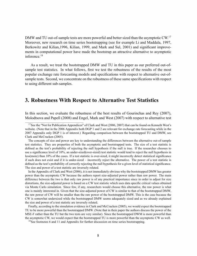
We test the robustness of their results with respect to different test statistics. In Table 1,we reproduce the monetary model results but rather than just report the asymptotic CW teststatistic, we also report the bootstrapped p-values of the DMW, TU, CW and ENC-NEW. Ifwe test statistical signi�cance via the bootstrapped DMW and TU test statistics, the p-value isless than 10% for only 4 out of 18 cases.24 These results are con�rmed by the bootstrapped21Engel, Mark and West (2007) compare the forecasts of the monetary model to both the random walk with

drift and without drift. However, they note that the driftless random walk outperforms the random walk with drift.All of the studies we are aware of that compare the driftless random walk to the random walk with drift, �nd thedriftless random walk to be a better forecaster (see Engel and Hamilton, 1990, and Engel, Mark and West, 2007).22For example, the normalization for France post 1999 will be simply franc/euro times euro/dollar where the

franc/euro is the peg used to �x the French franc to the euro in 1999.23We use Engel, Mark and West's (2007) data except for exchange rates which are from the IFS data set. The

bootstrap procedure is similar to Mark and Sul (2001) and assume no unit root of the monetary fundamental. (Fordetails on the bootstrap used see Appendix.)24Another way of testing for robustness, which we do not pursue in this paper, is by estimating to what extent

the positive results could be attributed to the large number of speci�cations tested. For instance, the test statisticintroduced byMcCracken and Sapp (2005) tests whether the number of successful forecasts can be attributed solelyto the large number of speci�cations and models estimated by the researcher. If we were to calculate McCrackenand Sapp's (2005) test statistic, the results might have been even less favorable for the structural models.

10

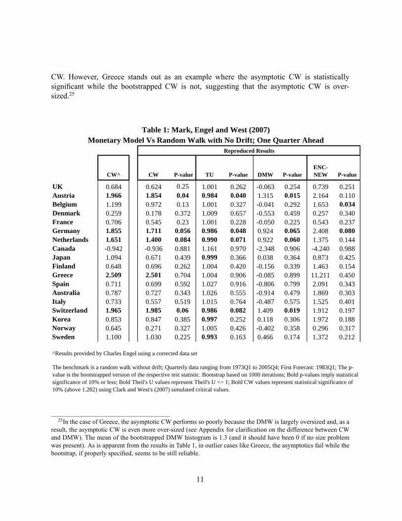
CW. However, Greece stands out as an example where the asymptotic CW is statisticallysigni�cant while the bootstrapped CW is not, suggesting that the asymptotic CW is over-sized.25

CW^ CW  P­value TU P­value DMW P­valueENC­NEW P­value

UK 0.684 0.624 0.25 1.001 0.262 ­0.063 0.254 0.739 0.251Austria 1.966 1.854 0.04 0.984 0.040 1.315 0.015 2.164 0.110Belgium 1.199 0.972 0.13 1.001 0.327 ­0.041 0.292 1.653 0.034Denmark 0.259 0.178 0.372 1.009 0.657 ­0.553 0.459 0.257 0.340France 0.706 0.545 0.23 1.001 0.228 ­0.050 0.225 0.543 0.237Germany 1.855 1.711 0.056 0.986 0.048 0.924 0.065 2.408 0.080Netherlands 1.651 1.400 0.084 0.990 0.071 0.922 0.060 1.375 0.144Canada ­0.942 ­0.936 0.881 1.161 0.970 ­2.348 0.906 ­4.240 0.988Japan 1.094 0.671 0.439 0.999 0.366 0.038 0.364 0.873 0.425Finland 0.648 0.696 0.262 1.004 0.420 ­0.156 0.339 1.463 0.154Greece 2.509 2.501 0.704 1.004 0.906 ­0.085 0.899 11.211 0.450Spain 0.711 0.699 0.592 1.027 0.916 ­0.806 0.799 2.091 0.343Australia 0.787 0.727 0.343 1.026 0.555 ­0.914 0.479 1.869 0.303Italy 0.733 0.557 0.519 1.015 0.764 ­0.487 0.575 1.525 0.401Switzerland 1.965 1.985 0.06 0.986 0.082 1.409 0.019 1.912 0.197Korea 0.853 0.847 0.385 0.997 0.252 0.118 0.306 1.972 0.188Norway 0.645 0.271 0.327 1.005 0.426 ­0.402 0.358 0.296 0.317Sweden 1.100 1.030 0.225 0.993 0.163 0.466 0.174 1.372 0.212

The benchmark is a random walk without drift; Quarterly data ranging from 1973Q1 to 2005Q4; First Forecast: 1983Q1; The p­value is the bootstrapped version of the respective test statistic. Bootstrap based on 1000 iterations; Bold p­values imply statisticalsignificance of 10% or less; Bold Theil's U values represent Theil's U <= 1; Bold CW values represent statistical significance of10% (above 1.282) using Clark and West's (2007) simulated critical values.

Reproduced Results

Monetary Model Vs Random Walk with No Drift; One Quarter AheadTable 1: Mark, Engel and West (2007)

^Results provided by Charles Engel using a corrected data set

25In the case of Greece, the asymptotic CW performs so poorly because the DMW is largely oversized and, as aresult, the asymptotic CW is even more over-sized (see Appendix for clari�cation on the difference between CWand DMW). The mean of the bootstrapped DMW histogram is 1.3 (and it should have been 0 if no size problemwas present). As is apparent from the results in Table 1, in outlier cases like Greece, the asymptotics fail while thebootstrap, if properly speci�ed, seems to be still reliable.

11

Molodtsova and Papell (2008) -Heterogeneous Symmetric Taylor Rule withSmoothing

In addition to the improvements produced by the panel speci�cation, the introduction of theTaylor rule as a structural fundamental has also seemed to yield improved forecasts. The speci-�cation which produces best forecasting results estimates country speci�c coef�cients on bothin�ation and the output gap. Furthermore, Molodtsova and Papell (2008) assume that inter-est rates adjust only partially to its target and, as a result, lagged interest rates are includedin the speci�cation which represent the so-called smoothing effect. Using only single-countryequations and the asymptotic CW test statistic, Molodtsova and Papell (2008) conclude that theTaylor rule outperforms the driftless random walk for 10 out of 12 currencies for forecasts oneperiod ahead. Molodtsova and Papell (2008) specify the fundamental, zt, as

zt = �1�t + �2��t + �3y

gapt + �4y

gap�t + �5it�1 + �6i

�t�1 (3)

where � is the in�ation rate, i is the interest rate and ygap is the output gap de�ned as the de-viation of an industrial production index from a linear trend. We substitute equation (3) inequation (1) and estimate equation (1) in a single equation framework using monthly data.26Molodtsova and Papell (2008) refer to speci�cation (3) as the heterogeneous symmetric Tay-lor rule with smoothing.27 More information regarding the speci�cation and data sources isprovided in Molodtsova and Papell (2008).

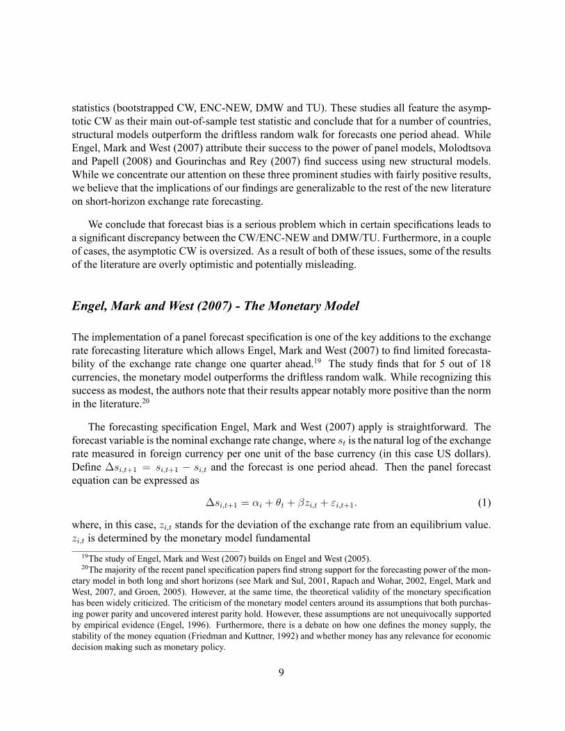
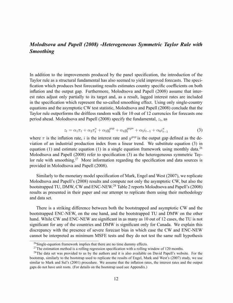
Similarly to the monetary model speci�cation of Mark, Engel and West (2007), we replicateMolodtsova and Papell's (2008) results and compute not only the asymptotic CW, but also thebootstrapped TU, DMW, CW and ENC-NEW.28 Table 2 reports Molodtsova and Papell's (2008)results as presented in their paper and our attempt to replicate them using their methodologyand data set.

There is a striking difference between both the bootstrapped and asymptotic CW and thebootstrapped ENC-NEW, on the one hand, and the bootstrapped TU and DMW on the otherhand. While CW and ENC-NEW are signi�cant in as many as 10 out of 12 cases, the TU is notsigni�cant for any of the countries and DMW is signi�cant only for Canada. We explain thisdiscrepancy with the presence of severe forecast bias in which case the CW and ENC-NEWcannot be interpreted as minimum MSFE tests and they do not test the same null hypothesis26Single-equation framework implies that there are no time dummy effects.27The estimation method is a rolling regression speci�cation with a rolling window of 120 months.28The data set was provided to us by the authors and it is also available on David Papell's website. For the

bootstrap, similarly to the bootstrap used to replicate the results of Engel, Mark and West's (2007) study, we usesimilar to Mark and Sul's (2001) procedure. We assume that the in�ation rates, the interest rates and the outputgaps do not have unit roots. (For details on the bootstrap used see Appendix.)

12

as TU and DMW.29 In the case of Switzerland, the bootstrapped CW is insigni�cant while theasymptotic CW is signi�cant, again, suggesting that the asymptotic CW might be oversized incertain cases.

Table 2: Molodtsova and Papell (2008)Heterogeneous Symmetric Taylor Rule with Smoothing Vs Random Walk with No Drift; One

Month Ahead

CW P­valueasymptotic^

CW P­value

asymptotic

CW P­value

bootstrap TUP­

value DMWP­

valueENC­NEW

P­value

UK 0.020 0.027 0.027 1.051 1.000 ­1.740 0.678 14.662 0.001Denmark 0.069 0.067 0.045 1.025 0.992 ­1.231 0.397 8.067 0.013France 0.024 0.019 0.007 1.040 0.998 ­1.260 0.557 11.312 0.001Germany 0.066 0.066 0.077 1.036 0.997 ­1.130 0.548 8.458 0.016Netherlands 0.036 0.035 0.040 1.040 1.000 ­1.304 0.613 9.604 0.012Canada 0.008 0.008 0.008 1.006 0.174 ­0.261 0.078 15.025 0.003Japan 0.019 0.019 0.071 1.018 0.912 ­0.723 0.367 14.152 0.008Australia 0.015 0.013 0.039 1.024 0.972 ­0.895 0.360 15.130 0.004Italy 0.002 0.002 0.039 0.995 0.264 0.168 0.327 18.240 0.003Switzerland 0.094 0.094 0.153 1.068 1.000 ­2.198 0.910 9.151 0.021Sweden 0.678 0.674 0.667 1.098 1.000 ­1.261 0.494 ­5.897 1.000Portugal 0.985 0.985 0.985 1.127 1.000 ­3.329 0.999 ­4.464 1.000^ Results as reported in Molodtsova and Papell (2008)

Single equation, monthly data. Since Molodtsova and Papell (2008)  use rolling regressions,  the asymptotic CW p­values arecalculated under the assuming of normality; The TU, ENC­NEW and DMW p­values and the CW  bootstrap p­value are based on abootstrap (1000 iterations); Bold Theil's U values represent Theil's U <= 1;

Gourinchas and Rey (2007) - External Balance Model

Another important study that claims to successfully forecast exchange rates one period ahead isGourinchas and Rey (2007). The authors introduce a new external balance model which isolateslong- term effects by de�ning an external balance variable as a function of de-trended foreignassets and liabilities, exports and imports. Gourinchas and Rey (2007) �nd that their externalbalance measure is superior to those previously used in the literature on external balance spec-i�cations since it takes into account capital gains and losses on the net foreign asset position,29A regression of the observed exchange rate change on the forecast series and no constant produces a coef�cient

less than or close to 0.5 for all 10 countries where CW and ENC-NEW are signi�cant. (If no "scale" forecast biaswas present, the coef�cient should have been close to 1.) This is what we would expect in cases of severe "scale"forecast bias which can lead to CW and ENC-NEW not testing the same null as TU and DMW.

13

in addition to the trade balance. Gourinchas and Rey (2007) argue that their external balancevariable successfully forecasts both the trade and FDI-weighted dollar one quarter ahead.

We can write Gourinchas and Rey's (2007) external balance fundamental as

zt = j�at j�at � j�ltj�lt + j�xt j�xt � j�mt j�mt (4)

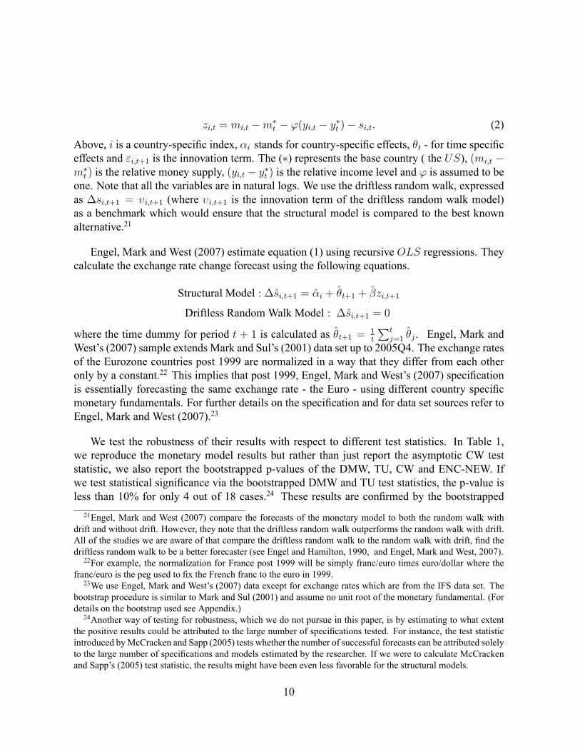
where �at ; �lt; �xt and �mt are time-varying weights � a function of the Hodrick-Prescott-�lteredtrends of assets, liabilities, exports and imports � while �at ; �lt; �xt and �mt represent the log devi-ation of assets, liabilities, exports and imports from Hodrick-Prescott-�ltered trends. Equation(4) is substituted into equation (1) and the authors estimate equation (1) for the trade-weightedand the FDI-weighted exchange rate separately in a single equation framework.30 Gourinchasand Rey (2007) assume that the time-varying weights converge asymptotically and use �xedweights for the calculation of their forecasts. Further details on the speci�cation and the dataset used are provided in Gourinchas and Rey (2007). In Table 3, we reproduce their results usingtheir data set and similar methodology.31 One can observe highly signi�cant asymptotic CW,bootstrapped TU, DMW, CW and ENC-NEW test statistics. However, the seemingly strongresult is overturned, to an extent, when checking for robustness with respect to alternative timeperiods in the following section.30Note that the authors claim to be using a 105 quarter rolling window. However, a closer look at their code

shows that they use 105 quarter rolling window for the forecasts of the FDI-traded dollar and a recursive speci�-cation for the trade-weighted dollar. We calculate the forecast both ways � in a recursive and rolling framework �and the results do not change substantially.31We are grateful to the authors for providing us with their code and data set. Note that in Table 3 we report

the CW test statistic which is calculated as CW = P 0:5dpdwhere d is de�ned in equation (6) in Appendix, while

Gorinchas and Rey (2007) report d in their paper.As before, we use a bootstrap procedure similar to Mark and Sul (2001) and assume no unit root of the external

balance variable. (For details on the bootstrap used see Appendix.)

14

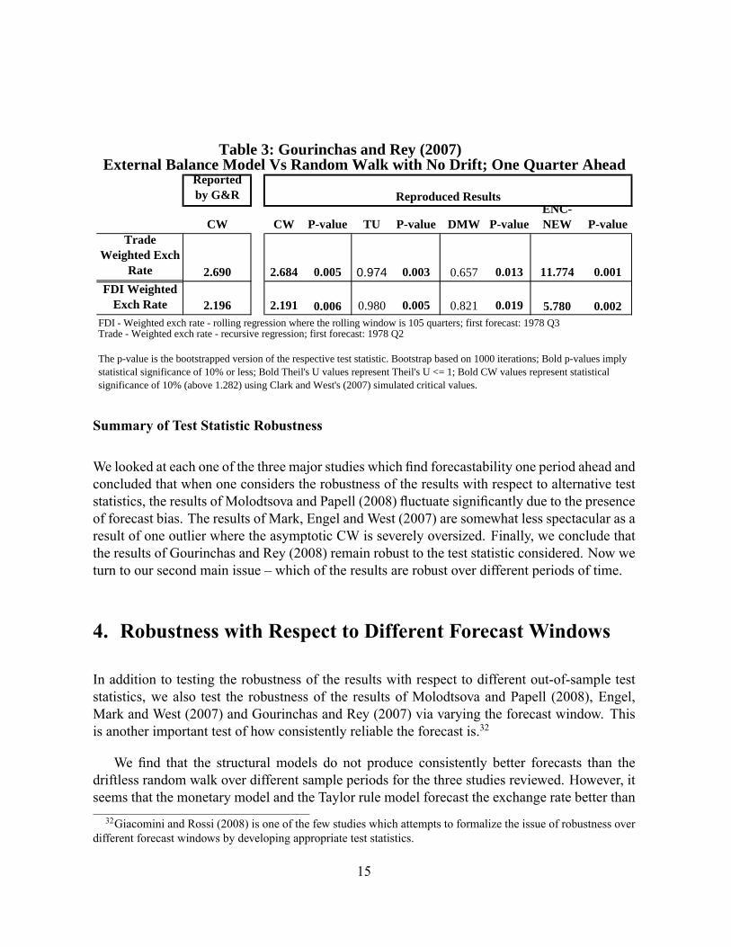
Reportedby G&R

CW CW P­value TU P­value DMW P­valueENC­NEW P­value

TradeWeighted Exch

Rate 2.690 2.684 0.005 0.974 0.003 0.657 0.013 11.774 0.001

0.006 5.780 0.002FDI ­ Weighted exch rate ­ rolling regression where the rolling window is 105 quarters; first forecast: 1978 Q3Trade ­ Weighted exch rate ­ recursive regression; first forecast: 1978 Q2

0.019

The p­value is the bootstrapped version of the respective test statistic. Bootstrap based on 1000 iterations; Bold p­values implystatistical significance of 10% or less; Bold Theil's U values represent Theil's U <= 1; Bold CW values represent statisticalsignificance of 10% (above 1.282) using Clark and West's (2007) simulated critical values.

External Balance Model Vs Random Walk with No Drift; One Quarter AheadTable 3: Gourinchas and Rey (2007)

FDI WeightedExch Rate 2.196 2.191 0.980 0.005 0.821

Reproduced Results

Summary of Test Statistic Robustness

We looked at each one of the three major studies which �nd forecastability one period ahead andconcluded that when one considers the robustness of the results with respect to alternative teststatistics, the results of Molodtsova and Papell (2008) �uctuate signi�cantly due to the presenceof forecast bias. The results of Mark, Engel and West (2007) are somewhat less spectacular as aresult of one outlier where the asymptotic CW is severely oversized. Finally, we conclude thatthe results of Gourinchas and Rey (2008) remain robust to the test statistic considered. Now weturn to our second main issue � which of the results are robust over different periods of time.

4. Robustness with Respect to Different Forecast Windows

In addition to testing the robustness of the results with respect to different out-of-sample teststatistics, we also test the robustness of the results of Molodtsova and Papell (2008), Engel,Mark and West (2007) and Gourinchas and Rey (2007) via varying the forecast window. Thisis another important test of how consistently reliable the forecast is.32

We �nd that the structural models do not produce consistently better forecasts than thedriftless random walk over different sample periods for the three studies reviewed. However, itseems that the monetary model and the Taylor rule model forecast the exchange rate better than32Giacomini and Rossi (2008) is one of the few studies which attempts to formalize the issue of robustness over

different forecast windows by developing appropriate test statistics.

15

the random walk during the 1980s while Gourinchas and Rey's (2007) external balance modelconsistently outperforms the driftless random walk in the 1990s and the 2000s.

Engel, Mark and West (2007)

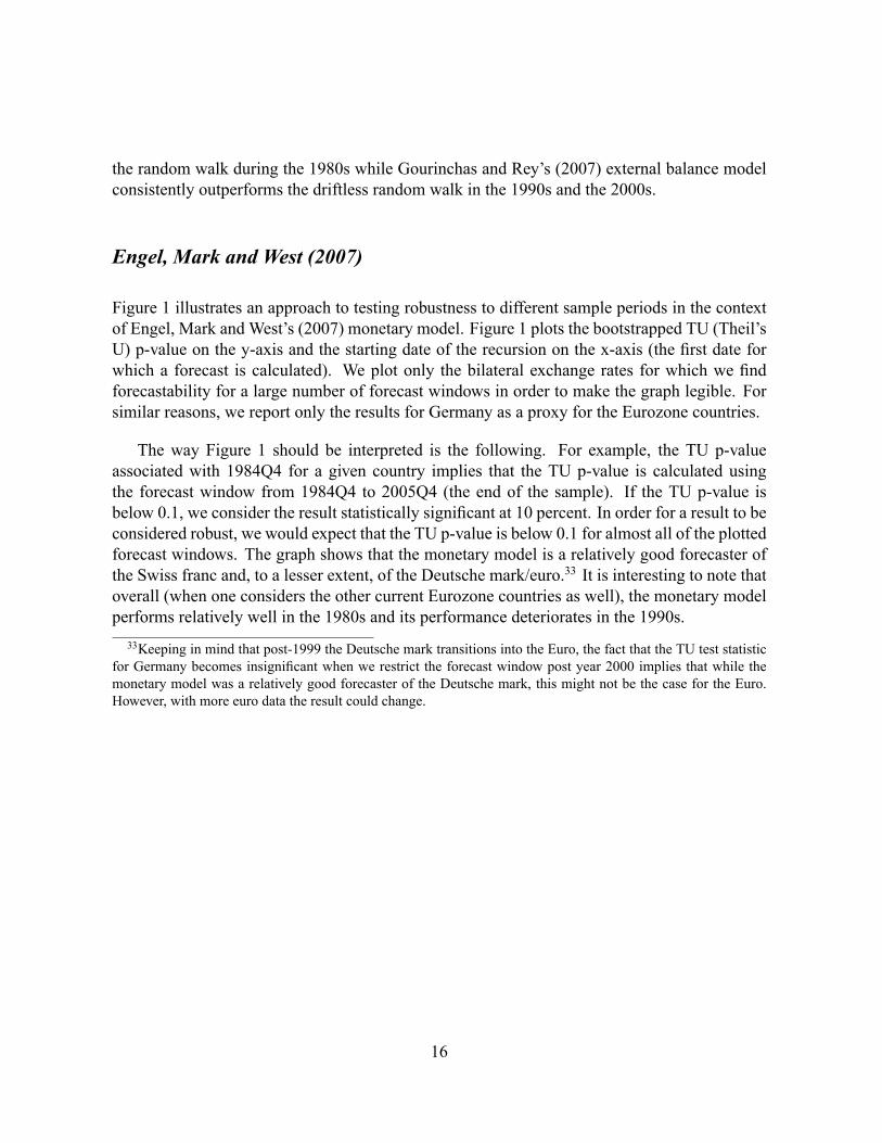
Figure 1 illustrates an approach to testing robustness to different sample periods in the contextof Engel, Mark and West's (2007) monetary model. Figure 1 plots the bootstrapped TU (Theil'sU) p-value on the y-axis and the starting date of the recursion on the x-axis (the �rst date forwhich a forecast is calculated). We plot only the bilateral exchange rates for which we �ndforecastability for a large number of forecast windows in order to make the graph legible. Forsimilar reasons, we report only the results for Germany as a proxy for the Eurozone countries.

The way Figure 1 should be interpreted is the following. For example, the TU p-valueassociated with 1984Q4 for a given country implies that the TU p-value is calculated usingthe forecast window from 1984Q4 to 2005Q4 (the end of the sample). If the TU p-value isbelow 0.1, we consider the result statistically signi�cant at 10 percent. In order for a result to beconsidered robust, we would expect that the TU p-value is below 0.1 for almost all of the plottedforecast windows. The graph shows that the monetary model is a relatively good forecaster ofthe Swiss franc and, to a lesser extent, of the Deutsche mark/euro.33 It is interesting to note thatoverall (when one considers the other current Eurozone countries as well), the monetary modelperforms relatively well in the 1980s and its performance deteriorates in the 1990s.33Keeping in mind that post-1999 the Deutsche mark transitions into the Euro, the fact that the TU test statistic

for Germany becomes insigni�cant when we restrict the forecast window post year 2000 implies that while themonetary model was a relatively good forecaster of the Deutsche mark, this might not be the case for the Euro.However, with more euro data the result could change.

16

In conclusion, while at �rst look (considering one forecast window only), Engel, Mark andWest's (2007) results seem encouraging, if one considers the robustness of the results overdifferent forecast windows, they are less so.34

Molodtsova and Papell (2008)

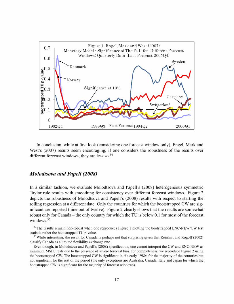
In a similar fashion, we evaluate Molodtsova and Papell's (2008) heterogeneous symmetricTaylor rule results with smoothing for consistency over different forecast windows. Figure 2depicts the robustness of Molodtsova and Papell's (2008) results with respect to starting therolling regression at a different date. Only the countries for which the bootstrapped CW are sig-ni�cant are reported (nine out of twelve). Figure 2 clearly shows that the results are somewhatrobust only for Canada � the only country for which the TU is below 0.1 for most of the forecastwindows.35

34The results remain non-robust when one reproduces Figure 1 plotting the bootstrapped ENC-NEW/CW teststatistic rather the bootstrapped TU p-value.35While interesting, the result for Canada is perhaps not that surprising given that Reinhart and Rogoff (2002)

classify Canada as a limited �exibility exchange rate.Even though, in Molodtsova and Papell's (2008) speci�cation, one cannot interpret the CW and ENC-NEW as

minimum MSFE tests due to the presence of severe forecast bias, for completeness, we reproduce Figure 2 usingthe bootstrapped CW. The bootstrapped CW is signi�cant in the early 1980s for the majority of the countries butnot signi�cant for the rest of the period (the only exceptions are Australia, Canada, Italy and Japan for which thebootstrapped CW is signi�cant for the majority of forecast windows).

17

Gourinchas and Rey (2007)

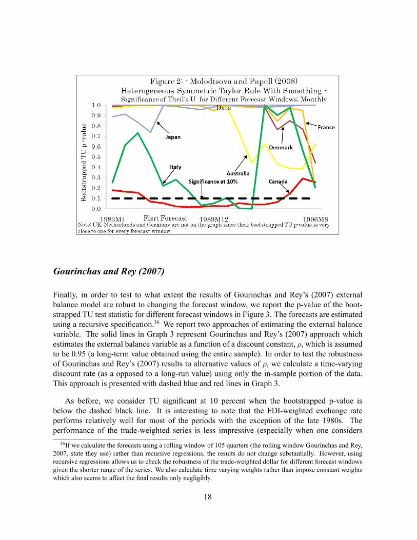
Finally, in order to test to what extent the results of Gourinchas and Rey's (2007) externalbalance model are robust to changing the forecast window, we report the p-value of the boot-strapped TU test statistic for different forecast windows in Figure 3. The forecasts are estimatedusing a recursive speci�cation.36 We report two approaches of estimating the external balancevariable. The solid lines in Graph 3 represent Gourinchas and Rey's (2007) approach whichestimates the external balance variable as a function of a discount constant, �, which is assumedto be 0.95 (a long-term value obtained using the entire sample). In order to test the robustnessof Gourinchas and Rey's (2007) results to alternative values of �, we calculate a time-varyingdiscount rate (as a opposed to a long-run value) using only the in-sample portion of the data.This approach is presented with dashed blue and red lines in Graph 3.

As before, we consider TU signi�cant at 10 percent when the bootstrapped p-value isbelow the dashed black line. It is interesting to note that the FDI-weighted exchange rateperforms relatively well for most of the periods with the exception of the late 1980s. Theperformance of the trade-weighted series is less impressive (especially when one considers36If we calculate the forecasts using a rolling window of 105 quarters (the rolling window Gourinchas and Rey,

2007, state they use) rather than recursive regressions, the results do not change substantially. However, usingrecursive regressions allows us to check the robustness of the trade-weighted dollar for different forecast windowsgiven the shorter range of the series. We also calculate time varying weights rather than impose constant weightswhich also seems to affect the �nal results only negligibly.

18

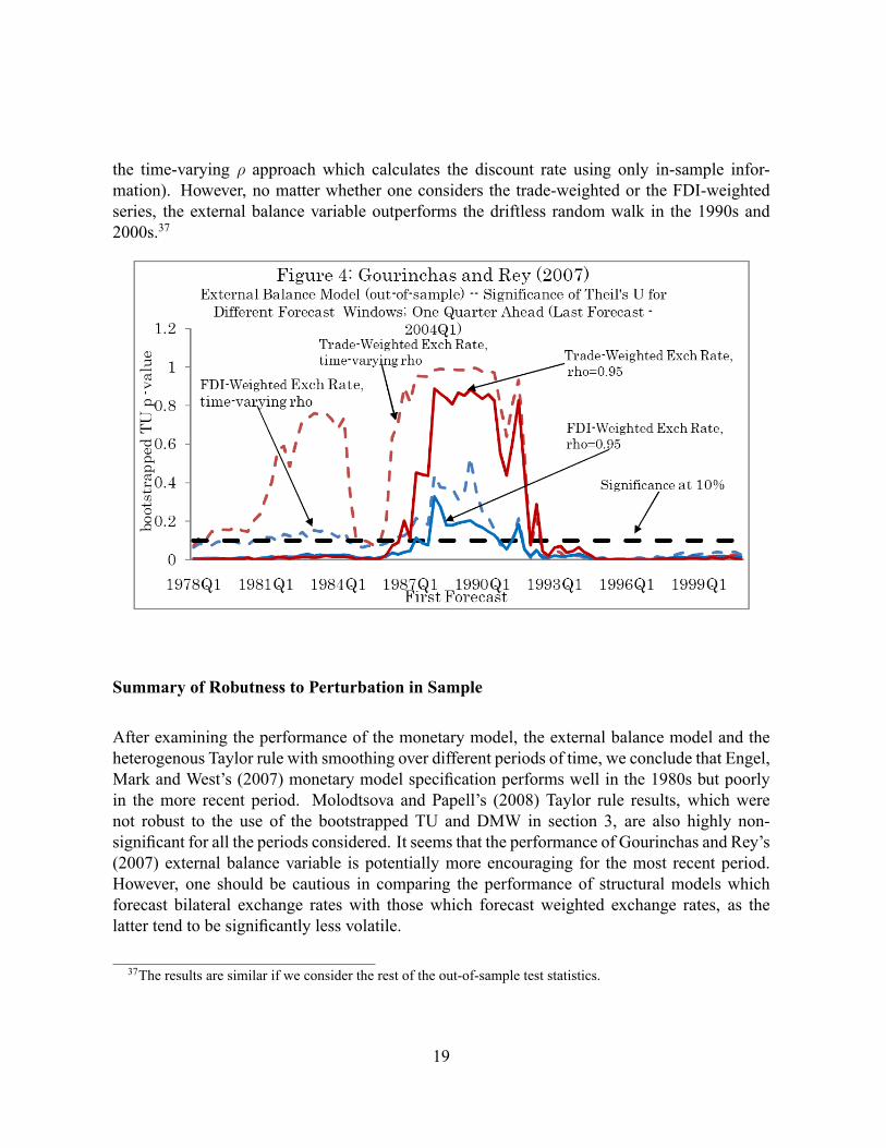
the time-varying � approach which calculates the discount rate using only in-sample infor-mation). However, no matter whether one considers the trade-weighted or the FDI-weightedseries, the external balance variable outperforms the driftless random walk in the 1990s and2000s.37

Summary of Robutness to Perturbation in Sample

After examining the performance of the monetary model, the external balance model and theheterogenous Taylor rule with smoothing over different periods of time, we conclude that Engel,Mark and West's (2007) monetary model speci�cation performs well in the 1980s but poorlyin the more recent period. Molodtsova and Papell's (2008) Taylor rule results, which werenot robust to the use of the bootstrapped TU and DMW in section 3, are also highly non-signi�cant for all the periods considered. It seems that the performance of Gourinchas and Rey's(2007) external balance variable is potentially more encouraging for the most recent period.However, one should be cautious in comparing the performance of structural models whichforecast bilateral exchange rates with those which forecast weighted exchange rates, as thelatter tend to be signi�cantly less volatile.

37The results are similar if we consider the rest of the out-of-sample test statistics.

19

5. Can One Do Better? The Importance of Common Cross-Country Shocks

In this section we try to improve upon the panel forecast speci�cation applied by Mark and Sul(2001) and Engel, Mark and West (2007) by incorporating persistent common cross-countryshocks in the forecasts. These might include technology shocks, commodity price shocks, orfactors related to the pace of globalization.

The basic forecast speci�cation we use is the same as the one de�ned in equation (1). How-ever, we de�ne zi;t, the deviation of the exchange rate from an equilibrium value, using thepurchasing power parity model (PPP) rather than the monetary model.38

zi;t = pi;t � p�t � si;t (5)

Above, p is the natural log of the CPI and, as before, the (�) represents the US. We substituteequation (5) into equation (1) and estimate equation (1) using recursive OLS panel regressions.The way we take into account potential persistent cross-country shocks is by forecasting thetime dummy effect for period t+1 differently from previous panel studies. Rather than forecastit simply as the average of the time-dummy coef�cients for all the previous periods, as Mark,Engel and West (2007) did, we forecast it as a simple average of the last 4 estimated time-dummy coef�cients. Mathematically, the time dummy forecast can be de�ned as

�t+1 =1

q

tXj=t�q+1

�j

where q = 4 when the data is quarterly.

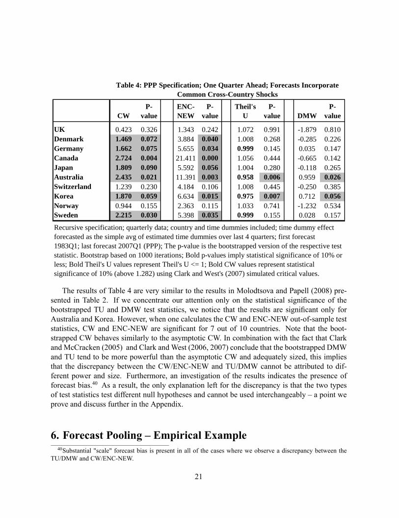
Table 4 reports the results of the speci�cation de�ned above. 39

38The PPP speci�cation is known to perform well at long horizons, but has been much less explored in lookingat short-horizon nominal exchange rate forecasts. Engel, Mark and West (2007) is the only study, we are awareof, which has explored the forecasting power of the PPP model at short horizons in a panel framework where thebenchmark is the driftless random walk. Engel, Mark and West (2007) �nd that for forecasts one period ahead, thePPP forecast is signi�cantly better than the driftless random walk forecast only in 3 out of 18 cases.We also perform the same type of forecasting exercise as in sections 5 and 6 using the monetary model, the

Taylor rule and a new structural model based on the Backus - Smith optimal risk sharing condition model. Out ofall the models we try, the PPP speci�cation performs the best.39The data source is the International Financial Statistics (IMF) (Data available upon request). Our data set

consists of eleven countries: US, UK, Denmark, Germany, Canada, Japan, Australia, Switzerland, Korea, Norwayand Sweden. We choose to proxy the Euro using the Deutsche mark series up to 1999 and the euro post 1999. Thebootstrap speci�cation is similar to Mark and Sul (2001) and the same as the bootstrap used in the literature reviewsection (see Appendix for details).

20

CWP­

valueENC­NEW

P­value

Theil'sU

P­value DMW

P­value

UK 0.423 0.326 1.343 0.242 1.072 0.991 ­1.879 0.810Denmark 1.469 0.072 3.884 0.040 1.008 0.268 ­0.285 0.226Germany 1.662 0.075 5.655 0.034 0.999 0.145 0.035 0.147Canada 2.724 0.004 21.411 0.000 1.056 0.444 ­0.665 0.142Japan 1.809 0.090 5.592 0.056 1.004 0.280 ­0.118 0.265Australia 2.435 0.021 11.391 0.003 0.958 0.006 0.959 0.026Switzerland 1.239 0.230 4.184 0.106 1.008 0.445 ­0.250 0.385Korea 1.870 0.059 6.634 0.015 0.975 0.007 0.712 0.056Norway 0.944 0.155 2.363 0.115 1.033 0.741 ­1.232 0.534Sweden 2.215 0.030 5.398 0.035 0.999 0.155 0.028 0.157

Recursive specification; quarterly data; country and time dummies included; time dummy effectforecasted as the simple avg of estimated time dummies over last 4 quarters; first forecast1983Q1; last forecast 2007Q1 (PPP); The p­value is the bootstrapped version of the respective teststatistic. Bootstrap based on 1000 iterations; Bold p­values imply statistical significance of 10% orless; Bold Theil's U values represent Theil's U <= 1; Bold CW values represent statisticalsignificance of 10% (above 1.282) using Clark and West's (2007) simulated critical values.

Table 4: PPP Specification; One Quarter Ahead; Forecasts IncorporateCommon Cross­Country Shocks

The results of Table 4 are very similar to the results in Molodtsova and Papell (2008) pre-sented in Table 2. If we concentrate our attention only on the statistical signi�cance of thebootstrapped TU and DMW test statistics, we notice that the results are signi�cant only forAustralia and Korea. However, when one calculates the CW and ENC-NEW out-of-sample teststatistics, CW and ENC-NEW are signi�cant for 7 out of 10 countries. Note that the boot-strapped CW behaves similarly to the asymptotic CW. In combination with the fact that Clarkand McCracken (2005) and Clark and West (2006, 2007) conclude that the bootstrapped DMWand TU tend to be more powerful than the asymptotic CW and adequately sized, this impliesthat the discrepancy between the CW/ENC-NEW and TU/DMW cannot be attributed to dif-ferent power and size. Furthermore, an investigation of the results indicates the presence offorecast bias.40 As a result, the only explanation left for the discrepancy is that the two typesof test statistics test different null hypotheses and cannot be used interchangeably � a point weprove and discuss further in the Appendix.

6. Forecast Pooling � Empirical Example40Substantial "scale" forecast bias is present in all of the cases where we observe a discrepancy between the

TU/DMW and CW/ENC-NEW.

21

However, a signi�cant CW/ENC-NEW still provides useful information when the bootstrappedTU/DMW is insigni�cant which is what one observes in Table 4 (For proof see Appendix). Inthis section we provide an empirical example of how in such cases one can improve upon thestructural model forecast by pooling the structural model forecast and the random walk forecast.

Endogenous vs Exogenous Weights

The question emerges how one can calculate a weight which will produce a forecast with MSFEsmaller than the MSFE of the random walk. One can either use endogenous time-varying meth-ods of �nding the optimal weight (see Clements and Hendry, 1998, pp. 229), or one can imposea �xed weight exogenously. It is conventional wisdom in the literature on forecast pooling thatsimple averages tend to outperform endogenous weights (See Stock and Watson, 2003, Clarkand McCracken, 2006 and Clements and Hendry, 2004). Clements and Hendry (2004) explainthis phenomena with the fact that all endogenous procedures of �nding an optimal weight wouldbe biased in the presence of structural breaks (which might be one explanation of the lack ofrobustness of the models over different forecast windows discussed in section 4).41 In contrast,having a constant weight can serve as an insurance against structural breaks and perform overallbetter than a time-varying endogenous weight.42

We test which pooling procedure produces better results � imposing exogenous �xed weightsor calculating endogenous weights using the regression method presented in Clements andHendry (1998, pp. 229). As expected, our results con�rm the conclusion of the literature onforecast pooling that simple means and �xed weights perform better than endogenously calcu-lated optimal weights. 43 As a result, we choose to impose a �xed weight of 0:2 on the structuralmodel forecast and 0:8 on the random walk forecast (which is essentially zero).44

41Since endogenous weights are estimated on the basis of data prior to the forecast, a structural break in therecent past or in the near future will lead to biased weights. It is possible that prior to the break, a certain modelperforms better than the alternative but performs poorly after the structural break. As a result, endogenouslydetermined weights would lead to the forecaster weighting more heavily the model which performed better priorto the break but poorly after it.42Potential structural breaks affect also the degree to which the information provided by the CW and the ENC-

NEW is valuable. In the presence of structural breaks, pooling can be appropriate even if the CW and the ENC-NEW are not statistically signi�cant (and of course the bootstrapped TU and DMW are not statistically signi�cant)(see Hendry and Clements, 2004). The reason why this is the case is that the forecaster does not know in advancewhether the CW/ENC-NEW will be signi�cant or not if the test statistic is calculated using data from the nextregime.43Results available upon request.44The results are relatively robust to using a simple average.

22

Results After Pooling

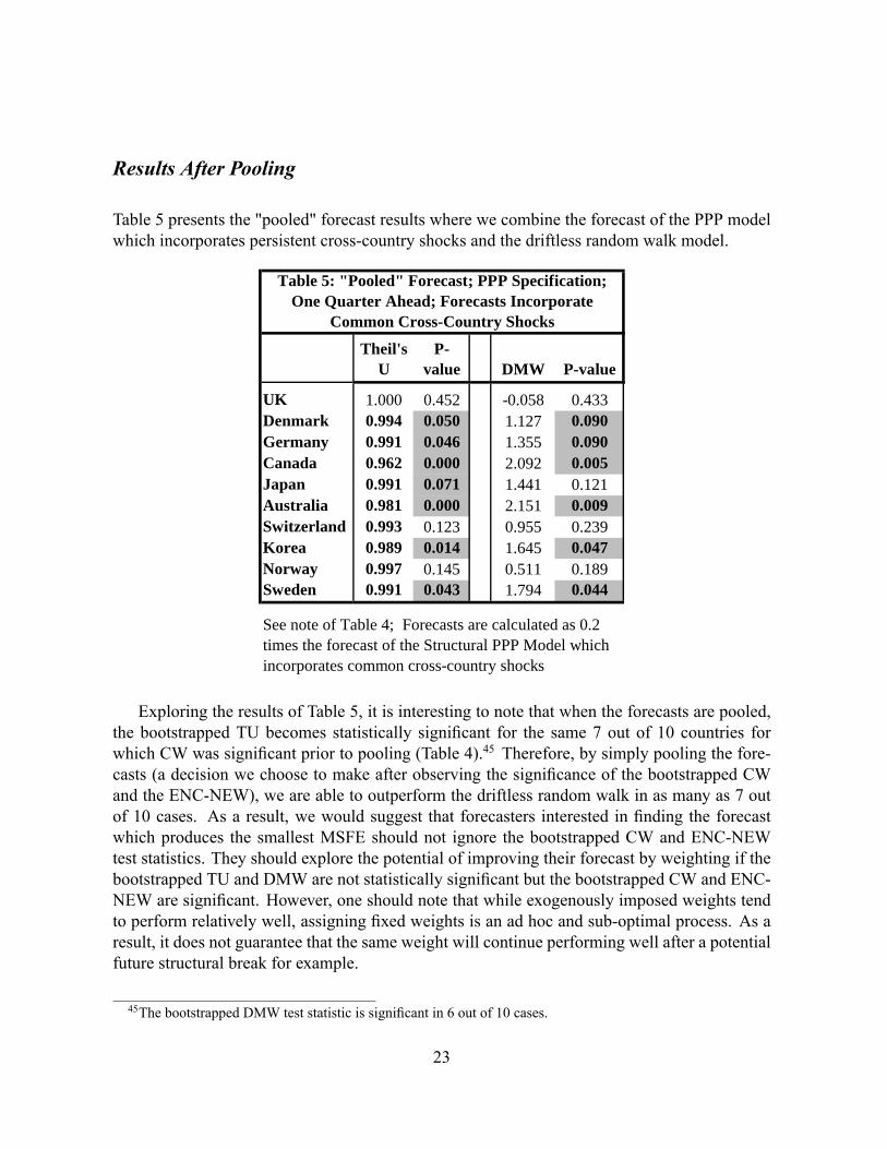
Table 5 presents the "pooled" forecast results where we combine the forecast of the PPP modelwhich incorporates persistent cross-country shocks and the driftless random walk model.

Theil'sU

P­value DMW P­value

UK 1.000 0.452 ­0.058 0.433Denmark 0.994 0.050 1.127 0.090Germany 0.991 0.046 1.355 0.090Canada 0.962 0.000 2.092 0.005Japan 0.991 0.071 1.441 0.121Australia 0.981 0.000 2.151 0.009Switzerland 0.993 0.123 0.955 0.239Korea 0.989 0.014 1.645 0.047Norway 0.997 0.145 0.511 0.189Sweden 0.991 0.043 1.794 0.044

Table 5: "Pooled" Forecast; PPP Specification;One Quarter Ahead; Forecasts Incorporate

Common Cross­Country Shocks

See note of Table 4;  Forecasts are calculated as 0.2times the forecast of the Structural PPP Model whichincorporates common cross­country shocks

Exploring the results of Table 5, it is interesting to note that when the forecasts are pooled,the bootstrapped TU becomes statistically signi�cant for the same 7 out of 10 countries forwhich CW was signi�cant prior to pooling (Table 4).45 Therefore, by simply pooling the fore-casts (a decision we choose to make after observing the signi�cance of the bootstrapped CWand the ENC-NEW), we are able to outperform the driftless random walk in as many as 7 outof 10 cases. As a result, we would suggest that forecasters interested in �nding the forecastwhich produces the smallest MSFE should not ignore the bootstrapped CW and ENC-NEWtest statistics. They should explore the potential of improving their forecast by weighting if thebootstrapped TU and DMW are not statistically signi�cant but the bootstrapped CW and ENC-NEW are signi�cant. However, one should note that while exogenously imposed weights tendto perform relatively well, assigning �xed weights is an ad hoc and sub-optimal process. As aresult, it does not guarantee that the same weight will continue performing well after a potentialfuture structural break for example.

45The bootstrapped DMW test statistic is signi�cant in 6 out of 10 cases.

23

Robustness of the Pooled Forecast with Respect to Different Forecast Win-dows - Is Pooling Enough?

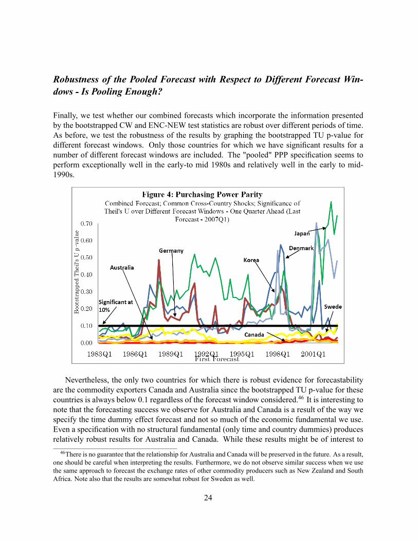
Finally, we test whether our combined forecasts which incorporate the information presentedby the bootstrapped CW and ENC-NEW test statistics are robust over different periods of time.As before, we test the robustness of the results by graphing the bootstrapped TU p-value fordifferent forecast windows. Only those countries for which we have signi�cant results for anumber of different forecast windows are included. The "pooled" PPP speci�cation seems toperform exceptionally well in the early-to mid 1980s and relatively well in the early to mid-1990s.

Nevertheless, the only two countries for which there is robust evidence for forecastabilityare the commodity exporters Canada and Australia since the bootstrapped TU p-value for thesecountries is always below 0.1 regardless of the forecast window considered.46 It is interesting tonote that the forecasting success we observe for Australia and Canada is a result of the way wespecify the time dummy effect forecast and not so much of the economic fundamental we use.Even a speci�cation with no structural fundamental (only time and country dummies) producesrelatively robust results for Australia and Canada. While these results might be of interest to46There is no guarantee that the relationship for Australia and Canada will be preserved in the future. As a result,

one should be careful when interpreting the results. Furthermore, we do not observe similar success when we usethe same approach to forecast the exchange rates of other commodity producers such as New Zealand and SouthAfrica. Note also that the results are somewhat robust for Sweden as well.

24

forecasters, they would most likely be of lesser value to policy makers who are interested in therelationship between structural models and fundamentals.47

Overview and Summary of PPP Model (with Common Cross-Country Shocks)

To summarize, panel forecast techniques should improve our ability to forecast exchange ratesby increasing the sample size and by allowing for cross-country interactions. We argue that,to an extent, forecasters can exploit cross-country interactions even further via specifying thetime dummy effect forecast in a way which captures world economic trends. However, whileallowing for the incorporation of cross-country information produces slight improvement oversimple panel speci�cations, it fails to produce robust results for the majority of the countriesconsidered. The only exceptions are the commodity producers � Canada and Australia � butwe caution the reader that further investigation of these "success" cases is required. Last butnot least, while alternative ways to forecast the time dummy or pooling the structural modelcoef�cient across countries may potentially improve our ability to forecast exchange rates forsome countries, one should be cautious when interpreting the results.48 If our ability to forecastexchange rates can be attributed solely to "ad hoc" procedures that take into account unknowncross-country shocks and common relationships, we still have not improved signi�cantly ourknowledge of the relationship between structural models and exchange rates.

Conclusion

In this paper we attempt to answer the question "Are structural models getting closer to beingable to forecast exchange rates at short horizons?" and the answer is "A little." However, over-reliance on asymptotic test statistics in out-of-sample comparisons, misinterpretation of sometests, and failure to suf�ciently check robustness to alternative time windows has led many stud-ies to overstate even the relatively thin positive results that have been found. We �nd that byallowing for common shocks in our panel speci�cation, we are able to generate some improve-ment, but even that improvement is not entirely robust to the forecast window, and much of thegain appears to come from non-structural rather than structural factors.47For example, while our results suggest that common cross-country shocks seem to forecast the exchange rates

of Australia and Canada relatively well, this result does not help policy makers determine the cause of these shocksor determine the relationship between structural variables and the exchange rate. A recent paper by Chen, Rogoffand Rossi (2008) is an example of the dif�culty of forecasting the exchange rates of commodity producers solelyusing fundamentals such as commodity prices even when one takes into account structural breaks.48For example, Rapach and Wohar (2004) provide empirical evidence against pooling the monetary model co-

ef�cient across countries.

25

We explore the application of popular new out of sample test statistics such as the Clarkand West (2006, 2007) and Clark and McCracken (2001) out-of-sample test statistics. We arguethat they have been widely misinterpreted as minimum mean square forecast error test statisticsand that, in addition, popular simple asymptotic versions may suffer from size distortions. Inother words, signi�cant Clark-West and Clark-McCracken test statistics do not always implythat the forecast of the structural model outperforms the forecast of the random walk in termsof mean square forecast error. For this question, statistics such as the bootstrapped Theil's U orDiebold-Mariano/West may be more appropriate (especially given the advances in time seriesbootstrapping); at the very least, researchers should test the robustness of their results withrespect to alternative test statistics.

We note that some researchers may be speci�cally interested in whether one can reject thenull hypothesis that the true model is the random walk model in favor a particular structuralmodel. But we would argue that in the vast majority of applications, policy-makers and practi-tioners treat the random walk model only as a straw man, and simply want to know whether thestructural model can deliver a better forecast and what that forecast is.

We do note that, in principle, a positive CW statistic implies that there does exist some linearcombination of the driftless random walk and the structural model that outperforms the naiverandom walk as measured by relative mean square forecast error. Finding a stable linear combi-nation, however, is tricky and potentially opens up a whole new range of problems. Endogenousmethods for �nding optimal weights tend to fail due to the presence of structural instability. Inpractice, �xed exogenous weights tend to perform better, although here too stability is a chal-lenge.

In addition to misinterpretation of the new out-of-sample tests for nested models, some ofthe excess optimism in the literature can be attributed to the failure to check for robustness overdifferent forecast windows. Regardless of whether one uses new or old structural models, singleequation or panel speci�cations, one of the main problems related to the forecastability of themajority of exchange rates remains - lack of robustness over different time periods. Whetherthe lack of robustness is due to non-linear functional forms, structural breaks or simply het-erogenous market sentiments over time49, the literature on exchange rate forecasting has notbeen able to develop the tools to produce robust forecasts for the majority of exchange rates.Innovative approaches of overcoming these problems are required in order for the forecasts of49One way of explaining the lack of robustness is with the existence of structural breaks which are identi�ed

as one of the main problems related to out-of-sample forecasting (see Clements and Hendry, 2005, Rossi, 2005,Stock and Watson, 1996, 2003). Potential model mis-speci�cation could be an alternative explanation. Empiricalevidence suggest that the relationship between fundamentals and exchange rates can be better represented bynon-linear rather than linear functional forms (see Taylor and Peel, 2000, Meese and Rose, 1991 and Kilian andTaylor, 2001). However, even when forecasters try to account for non-linear functional forms directly (Meese andRose,1991, and Killian and Taylor, 2001), or estimate a regime switching model (Marsh, 2000, and Dacco andSatchell, 1999), results remain non-robust.

26

structural models to outperform the forecasts of the driftless random walk at short-horizons.Until then, we would call the glass ninety-�ve percent empty rather than �ve percent full.

ReferencesAlquist, R., and M. Chinn (2006), "Conventional and Unconventional Approaches to ExchangeRate Modeling and Assessment", NBERWorking Paper No.12481.

Ardic, O. P., O. Ergin and G. B. Senol (2008), "Exchange Rate Forecasting: Evidence fromthe Emerging Central and Eastern European Economies", mimeo, Bogazici University.

Basher, S., and J. Westerlund (2006), "Can Panel Data Really Improve the Predictability ofthe Monetary Exchange Rate Model?", MPRAWorking Paper No. 1229.

Berkowitz, J., and L. Kilian (1996), "Recent Developments in Bootstrapping Time Series,"FEDS Discussion Paper No. 96-45.

Boucher, C. (2006), "Stock Prices � In�ation Puzzle and the Predictability of Stock MarketReturns", Economics Letters 90(2), 205-212.

Brownstone, D., and B. Valletta (2001), "The Bootstrap and Multiple Imputations: Har-nessing Increased Computing Power for Improved Statistical Tests", The Journal of EconomicPerspectives 15(4),129-141.

Cerra, V., and S. C. Saxena (2008), "The Monetary Model Strikes Back: Evidence from theWorld", IMF Working Paper Series WP/08/73.

Chen,Y., K. Rogoff and B. Rossi (2008), "Can Exchange Rates Forecast Commodity Prices?",mimeo, Harvard University.

Cheung, Y.-W., M. Chinn and A. Pascual (2003), "Empirical Exchange Rate Models of theNineties: Are Any�t to Survive?", mimeo, University of California at Santa Cruz.

27

Chong, Y., and D. Hendry (1986), " Econometric Evaluation of Linear Macro-EconomicsModels", Review of Economics Studies 53, 671-690.

Clark, T., and K. West (2006), "Using Out-of-Sample Mean Squared Prediction Errors toTest the Martingale Difference Hypothesis", Journal of Econometrics 135, 155-186.

Clark, T., and K. West (2007), "Approximately Normal Tests for Equal Predictive Accuracyin Nested Models", Journal of Econometrics 138, 291-311.

Clark, T., and M. McCracken (2001), "Tests of Equal Forecast Accuracy and Encompassingfor Nested Models", Journal of Econometrics 105, 85�110.

Clark, T., and M. McCracken (2005), "Evaluating Direct Multi-Step Forecasts", Economet-ric Reviews 24(4), 369�404.

Clements, M., and D. Hendry (1993), " On the Limitations of Comparing Mean SquareForecast Errors", Journal of Forecasting 12, 617-637.

Clements, M., and D. Hendry (1996), "Intercept Corrections and Structural Change", Jour-nal of Applied Econometrics 11, 475-494.

Clements, M., and D. Hendry (1998), "Forecasting Economic Time Series", CambridgeUniversity Press.

Clements, M., and D. Hendry (1999), "Forecasting Non-Stationary Economic Time Series",Cambridge University Press.

Clements, M., and D. Hendry (2004), "Pooling of Forecast", Econometrics Journal 7(1),1-31.

Clements, M., and D. Hendry (2005), "Forecasting with Breaks", in Elliott, G., C. Grangerand A. Timmermann (ed.),Handbook of Economic Forecasting, Elsevier, 1(1),1, 605-657 (2006).

Dacco, R., and S. Satchell (1999), �Why Do Regime-SwitchingModels Forecast So Badly?�,Journal of Forecasting 18, 1-16.

Diebold, F., and R. Mariano (1995), �Comparing Predictive Accuracy�, Journal of Businessand Economic Statistics 13, 253-265.

Efron, B. (1979), �Bootstrap Methods: Another Look at the Jackknife,� Annals of Statistics9, 1218-1228.

Engel, C. (1996), "The Forward Discount Anomaly and the Risk Premium: A Survey ofRecent Evidence", Journal of Empirical Finance 3, 123�191.

28

Engel, C., and J. Hamilton (1990), "Long Swings in the Exchange Rate: Are They in theData and Do Markets Know It?", American Economic Review 80 (4), 689-713.

Engel, C. and K. West (2005), "Exchange Rates and Fundamentals," Journal of PoliticalEconomy 113 (3), 485-517.Engel, C., Mark, N. and K. West (2007), "Exchange Rate Models Are Not as Bad as You

Think," NBER Macroeconomics Annual.

Ericsson, N. (1992), "Parameter Constancy, Mean Square Forecast Errors, and MeasuringForecast Performance: An Exposition, Extensions, and Illustration," Journal of Policy Modeling14 (4), 465-495.

Franses, P., and R. Legerstee (2007), "Does Experts Adjustment to Model-Based ForecastsContribute to Forecast Quality?" Econometric Instititute Report 37.

Friedman, B., and K. Kuttner (1992), "Money, Income and Prices After the 1980s," NBERWorking Papers 2852.

Giacomini, R., and B. Rossi (2006), "How Stable is the Forecasting Performance of theYield Curve for Output Growth?" Oxford Bulletin of Economics and Statistics 68, 783-795.

Giacomini, R., and B. Rossi (2008), "Forecast Comparisons in Unstable Environments",mimeo, Duke University.

Gourinchas, P.-O., and H. Rey (2007). "International Financial Adjustment," Journal ofPolitical Economy 115, 4.

Groen, J. (2005), "Exchange Rate Predictability and Monetary Fundamentals in a SmallMulti-Country Panel", Journal of Money, Credit and Banking 37, 495-516.

Groen, J. (2007), "Fundamentals Based Exchange Rate Prediction Revisited", mimeo, Fed-eral Reserve Bank of New York.

Harvey,D., and P. Newbold (1998), " Tests for Forecast Encompassing." Journal of Businessand Economic Statistics 16, 2.

Holden, K., and D. A. Peel (1989), "Unbiasedness, Ef�ciency and the Combination of Eco-nomic Forecasts." Journal of Forecasting 8, 175-188.Kilian, L. (1999), �Exchange Rates and Monetary Fundamentals: What Do We Learn from

Long-Horizon Regressions?�, Journal of Applied Econometrics 14, 491-510.

Kilian, L., and M. Taylor (2003), "Why Is It So Dif�cult to Beat the RandomWalk Forecastof Exchange Rates?", Journal of International Economics 60, 85-107.

29

Li, H. and Maddala, G. (1997), "Bootstrapping Cointegrating Regressions", Journal ofEconometrics, 80 (2), 297-318.

Maddala, G. and I.-M. Kim (1998),Unit Roots, Cointegration and Structural Change, Cam-bridge University Press.

MacKinnon,J. (2002), "Bootstrap Inference in Econometrics", Canadian Journal of Eco-nomics, 35 (4), 615-645.

Marcellino, M. (2000), �Forecast Bias and MSFE encompassing�, Oxford Bulletin of Eco-nomics and Statistics, 62, 533-542.

Mark, N. (1995), �Exchange Rates and Fundamentals: Evidence on Long Horizon Pre-dictability�, American Economic Review, 85, 201-218.

Mark, N., and D. Sul (2001), "Nominal Exchange Rates and Monetary Fundamentals: Ev-idence from a Small Post-Bretton Woods Sample", Journal of International Economics, 53,29-52.

Marsh, I. (2000), �High-Frequency Markov Switching Models in the Foreign ExchangeMarket�, Journal of Forecasting 19, 123-134.

McCracken, M. (1999), "Asymptotics for out of sample tests of causality", mimeo, Univer-sity of Missouri.

McCracken, M., and S. Sapp (2005), �Evaluating the Predictability of Exchange Rates Us-ing Long Horizon Regressions: Mind Your p's and q's!�, Journal of Money, Credit and Banking37, 473-494.

Meese, R., and K. Rogoff (1983a), �Empirical Exchange Rate Models of the Seventies: DoThey Fit Out of Sample?�, Journal of International Economics 14, 3-24.

Meese, R., and K. Rogoff (1983b), "The Out-of-Sample Failure of Empirical Exchange RateModels: Sampling Error or Misspeci�cation," in Jacob A. Frenkel, (ed.), Exchange Rates andInternational Macroeconomics, NBER.

Meese, R., and A. Rose (1991), "An Empirical Assessment of Non-Linearities in Models ofExchange Rate Determination", The Review of Economic Studies 58 (3), 603-619.

Molodtsova, T., and D. Papell (2008), "Out-of-Sample Exchange Rate Predictability withTaylor Rule Fundamentals", mimeo, University of Houston.

Molodtsova,T., A. Nikolsko-Rzhevskyy and D. Papell (2007), "Taylor Rules with Real-TimeData: A Tale of Two Countries and One Exchange Rate," mimeo, University of Houston.

30

Molodtsova,T., A. Nikolsko-Rzhevskyy and D. Papell (2008), "Taylor Rules and the Euro,"mimeo, University of Houston.

Politis, D., and H. White (2004), "Automatic Block-Length Selection for the DependentBootstrap," Econometric Reviews 23(1), 53 - 70.

Rapach,J., M. Wohar and D. Rangvid (2005), "Macro variables and international stock re-turn predictability", International Journal of Forecasting 21 (1), 137-166.

Rapach, D., J. Strauss and M. Wohar (2007), "Forecasting Stock Return Volatility in thePresence of Structural Breaks", in David E. Rapach and Mark E. Wohar (eds.), Forecasting inthe Presence of Structural Breaks and Model Uncertainty, Amsterdam: Elsevier, forthcoming.

Rapach, D., and M. Wohar (2002), "Testing the Monetary Model of Exchange Rate De-termination: New Evidence from a Century of Data," Journal of International Economics 58,359-385.

Rapach, D., and M. Wohar (2004), "Testing the Monetary Model of Exchange Rate Deter-mination: A Closer Look at Panels", Journal of International Money and Finance 23, 867-895.

Reinhart, C., and K. Rogoff (2002), "The Modern History of Exchange Rate Arrangements:A Reinterpretation", NBERWorking Paper.

Rossi, B. (2006), "Are Exchange Rates Really Random Walks? Some Evidence Robust toParameter Instability", Macroeconomic Dynamics 10(1), 20-38.

Sellin, P. (2006), "Using a Real Exchange Rate Model to Make Real and Nominal Fore-casts", mimeo, Sveriges Riksbank.

Stock, J., and M. Watson (1996), " Evidence of Structural Instability in MacroeconomicTime Series Relations", Journal of Business and Economic Statistics 14, 11-30.

Stock, J., and M. Watson (2003), "Forecasting Output and In�ation: The Role of AssetPrices", Journal of Economic Literature XLI, 788-829.

Taylor, M., and D. Peel (2000), "Nonlinear adjustment, long-run equilibrium and exchangerate fundamentals", Journal of International Money and Finance 19(1),33-53.

Zagaglia, P. (2006), "The Predictive Power of the Yield Spread under the Veil of Time",Stockholm University, Research Papers in Economics No 4.

West, K. (1996), "Asymptotic Inference About Predictive Ability", Econometrica 64, 1067-1084.

31

APPENDIX:

A. Minimum MSFE Out-of-Sample Test Statistics

The Theil's U Test (TU)

The TU test statistic is a minimum MSFE test de�ned as the square root of the MSFE of thestructural model over the square root of the MSFE of the random walk model. Therefore, aTU < 1 implies that the structural model outperforms the random walk model. TU is oftenpreferred for its simplicity and intuitive interpretation and its statistical signi�cance is tested viaa bootstrap. The test we use is a one-sided test.

The Diebold � Mariano/West Test (DMW)

The DMW test statistic can be considered an alternative to the TU test. It measures the statisti-cal signi�cance of the difference between the MSFE of the random walk model and that of thestructural model. A signi�cant and positive DMW test implies that the structural model outper-forms the random walk. On the basis of both theoretical and simulation evidence, West (1996),McCracken (1999), Clark and McCracken (2001, 2005) and Clark and West (2006) show that,when comparing nested models, the asymptotic DMW test statistic is undersized, which meansthat it may not detect statistical signi�cance (i.e., that the structural model outperforms the ran-dom walk model) even when it exists. While Clark and West (2006) attribute the poor sizeof the asymptotic DMW test statistic to small-sample bias, McCracken (1999) and Clark andMcCracken (2001, 2005) claim that the asymptotic DMW is undersized because the limitingdistribution of the DMW under the null hypothesis is not standard normal when nested modelsare compared. To correct for this problem, a number of studies opt for the bootstrapped DMWtest statistic which does not assume any distributional form. This is the approach we take in thispaper. Again, we calculate the DMW test as a one sided test.

The Clark � West Test (CW)

To compensate for the fact that the asymptotic DMW test statistic is undersized under the nullhypothesis when comparing nested models and to avoid the use of a bootstrap, Clark and West(2006, 2007) propose a new asymptotic test for nested models, the CW, that builds on theasymptotic DMW test. The CW test statistic takes into account the fact that the two modelscompared are nested by assuming that, under the null hypothesis, the exchange rate follows arandom walk.

32

When the forecast is calculated using rolling regressions, the limiting distribution of theCW under the null hypothesis is standard normal. However, when the estimation is performedrecursively, the asymptotic distribution is approximated using Brownian motion. Based on sim-ulation evidence, Clark and West (2007) suggest that, for recursive speci�cations, one can usea one-sided test and should reject the null hypothesis of equal forecasting power when the CW= +1:282 at 10 percent and CW = +1:645 at 5 percent (which are the critical values onewould use assuming a normal distribution). Finally, we also calculate the bootstrapped CW teststatistic to test whether the asymptotic CW test is properly sized.

The Clark - McCracken Test (ENC-NEW)

Another relatively new out-of-sample test statistic for nested models, the ENC-NEW, intro-duced by Clark and McCracken (2001, 2005), also implicitly assumes that, under the null, theexchange rate follows a random walk.50 The ENC-NEW and the CW differ only by a scalingfactor. In other words, the two test statistics can differ slightly because of different power orsize but they test the same null hypothesis. The shortcoming of the ENC-NEW is that its as-ymptotic distribution is a function of both the in-sample and out-of-sample portion of the datawhich makes evaluation of statistical signi�cance quite cumbersome. Therefore, bootstrappingthe ENC-NEW is an attractive alternative and this is the approach we take in this paper.

B. Proofs: The New Out-of-Sample Tests for Nested Models

In this section of the Appendix we provide a theoretical argument why the CW and ENC-NEWcannot be considered minimum MSFE tests in cases of severe "scale" forecast bias. We alsoargue that one should interpret these out-of-sample tests for nested models as prior tests ofwhether one can pool the random walk and the structural model forecast to produce a forecastwith MSFE signi�cantly smaller than the MSFE of the random walk.

50Similarly to the CW, the ENC-NEW has been one of the most widely used out-of-sample test statistics in theexchange rate forecasting literature. Some of the studies that test out-of-sample forecastability using the ENC-NEW are Franses and Legerstee (2007), Rossi (2006), Zagaglia (2006), Boucher (2006), Giacomini and Rossi(2006), Rangvid, Rapach, Wohar (2005).

33

From the Diebold � Mariano to the Clark � West Test

Before proceeding to the proofs, we present a derivation of the Clark and West test statistic,as presented in Clark andWest (2006). In order to simplify the notation, assume that the forecastis one period ahead and that the forecast variable is the change in the exchange rate. Assumethat yt = st � st�1; where st is the natural log of the exchange rate for period t: Also let Xt

be a matrix of explanatory variables. We are interested in comparing the forecasting power ofthe following theoretical models:

Driftless Random Walk Model: yt = e1;t; andStructural Model: yt = Xt�1b+ e2;t;

where e1;t and e2;t are the unobservable innovation terms.

The CW test assumes that, under the null hypothesis, the exchange rate is a random walk,and therefore, the population parameter b = 0; and the forecast innovation terms are equal,that is, e1;t+1 = e2;t+1. The models can be estimated by OLS using either recursive or rollingregressions. The estimated forecasts for the random walk and the structural model are y1;t+1 =0 and y2;t+1 = Xtbt respectively. Denoting P as the number of forecasts, T as the sample length,andR as the sample reserved to calculate the �rst forecast, we can rewrite the sample differencebetween the MSFE of the two models (which is the main component of the DMW test statistic)as:

P�1t=TXt=R+1

e21;t+1 � P�1t=TXt=R+1

e22;t+1 = 2P�1

t=TXt=R+1

(yt+1Xtbt)� P�1t=TXt=R+1

(Xtbt)2:

Clark and West (2006, 2007) argue that under the null hypothesis e1;t+1 = e2;t+1 = yt+1;and since Clark and West (2006, 2007) assume that the independent variables are not correlatedwith the theoretical disturbance terms, it follows that E(yt+1Xtbt) = 0:

51 Therefore, they arguethat we should expect

Pt=Tt=R+1(yt+1Xtbt) � 0 for both the rolling and recursive speci�cations.

However, due to small-sample bias, �P�1Pt=T

t=R+1(Xtbt)2 < 0: As a result, the sample differ-

ence of the MSFEs of the random walk and the structural model is negatively biased in favor ofthe random walk.

The fact that the DMW test is negatively biased under the null hypothesis implies that it fa-vors the random walk. Therefore, Clark and West (2006) propose an "adjusted" DMW statistic,or the so-called CW statistic, which tests whether51e1;t+1 = e2;t+1 implies E(yt+1Xtbt) = E(e1;t+1Xtbt) = E(e2;t+1Xtbt). By assumption, E(e2;t+1Xt) =

0. Then if one assumed that underlying variables are independent, E(e2;t+1Xtbt) = E(e2;t+1Xt)E(bt) = 0:

34

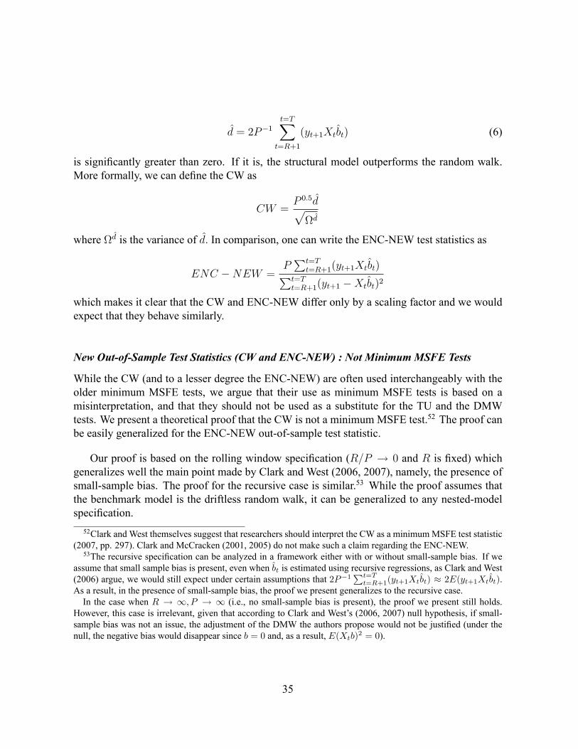
d = 2P�1t=TXt=R+1

(yt+1Xtbt) (6)

is signi�cantly greater than zero. If it is, the structural model outperforms the random walk.More formally, we can de�ne the CW as

CW =P 0:5dpd

where d is the variance of d: In comparison, one can write the ENC-NEW test statistics as

ENC �NEW =PPt=T

t=R+1(yt+1Xtbt)Pt=Tt=R+1(yt+1 �Xtbt)2

which makes it clear that the CW and ENC-NEW differ only by a scaling factor and we wouldexpect that they behave similarly.

New Out-of-Sample Test Statistics (CW and ENC-NEW) : Not Minimum MSFE Tests

While the CW (and to a lesser degree the ENC-NEW) are often used interchangeably with theolder minimum MSFE tests, we argue that their use as minimum MSFE tests is based on amisinterpretation, and that they should not be used as a substitute for the TU and the DMWtests. We present a theoretical proof that the CW is not a minimum MSFE test.52 The proof canbe easily generalized for the ENC-NEW out-of-sample test statistic.

Our proof is based on the rolling window speci�cation (R=P ! 0 and R is �xed) whichgeneralizes well the main point made by Clark and West (2006, 2007), namely, the presence ofsmall-sample bias. The proof for the recursive case is similar.53 While the proof assumes thatthe benchmark model is the driftless random walk, it can be generalized to any nested-modelspeci�cation.52Clark and West themselves suggest that researchers should interpret the CW as a minimumMSFE test statistic

(2007, pp. 297). Clark and McCracken (2001, 2005) do not make such a claim regarding the ENC-NEW.53The recursive speci�cation can be analyzed in a framework either with or without small-sample bias. If we

assume that small sample bias is present, even when bt is estimated using recursive regressions, as Clark and West(2006) argue, we would still expect under certain assumptions that 2P�1

Pt=Tt=R+1(yt+1Xtbt) � 2E(yt+1Xtbt).

As a result, in the presence of small-sample bias, the proof we present generalizes to the recursive case.In the case when R ! 1; P ! 1 (i.e., no small-sample bias is present), the proof we present still holds.

However, this case is irrelevant, given that according to Clark and West's (2006, 2007) null hypothesis, if small-sample bias was not an issue, the adjustment of the DMW the authors propose would not be justi�ed (under thenull, the negative bias would disappear since b = 0 and, as a result, E(Xtb)2 = 0).

35

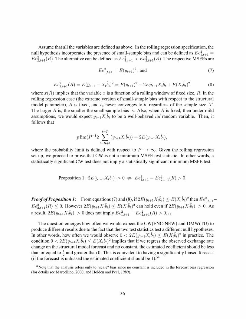
Assume that all the variables are de�ned as above. In the rolling regression speci�cation, thenull hypothesis incorporates the presence of small-sample bias and can be de�ned as Ee21;t+1 =Ee22;t+1(R): The alternative can be de�ned as Ee21;t+1 > Ee22;t+1(R): The respective MSFEs are

Ee21;t+1 = E(yt+1)2; and (7)

Ee22;t+1(R) = E(yt+1 �Xtbt)2 = E(yt+1)

2 � 2Eyt+1Xtbt + E(Xtbt)2; (8)

where x(R) implies that the variable x is a function of a rolling window of �xed size, R: In therolling regression case (the extreme version of small-sample bias with respect to the structuralmodel parameter), R is �xed, and bt never converges to b; regardless of the sample size, T:The larger R is, the smaller the small-sample bias is. Also, when R is �xed, then under mildassumptions, we would expect yt+1Xtbt to be a well-behaved iid random variable. Then, itfollows that

p lim(P�12t=TXt=R+1

(yt+1Xtbt)) = 2E(yt+1Xtbt);

where the probability limit is de�ned with respect to P ! 1: Given the rolling regressionset-up, we proceed to prove that CW is not a minimum MSFE test statistic. In other words, astatistically signi�cant CW test does not imply a statistically signi�cant minimum MSFE test.

Proposition 1: 2E(yt+1Xtbt) > 0 ; Ee21;t+1 � Ee22;t+1(R) > 0:

Proof of Proposition 1: From equations (7) and (8), if 2E(yt+1Xtbt) � E(Xtbt)2 thenEe21;t+1�

Ee22;t+1(R) � 0. However 2E(yt+1Xtbt) � E(Xtbt)2 can hold even if 2E(yt+1Xtbt) > 0. As

a result, 2E(yt+1Xtbt) > 0 does not imply Ee21;t+1 � Ee22;t+1(R) > 0: �

The question emerges how often we would expect the CW(ENC-NEW) and DMW(TU) toproduce different results due to the fact that the two test statistics test a different null hypotheses.In other words, how often we would observe 0 < 2E(yt+1Xtbt) � E(Xtbt)

2 in practice. Thecondition 0 < 2E(yt+1Xtbt) � E(Xtbt)

2 implies that if we regress the observed exchange ratechange on the structural model forecast and no constant, the estimated coef�cient should be lessthan or equal to 1

2and greater than 0. This is equivalent to having a signi�cantly biased forecast

(if the forecast is unbiased the estimated coef�cient should be 1).54

54Note that the analysis refers only to "scale" bias since no constant is included in the forecast bias regression(for details see Marcellino, 2000, and Holden and Peel, 1989).

36

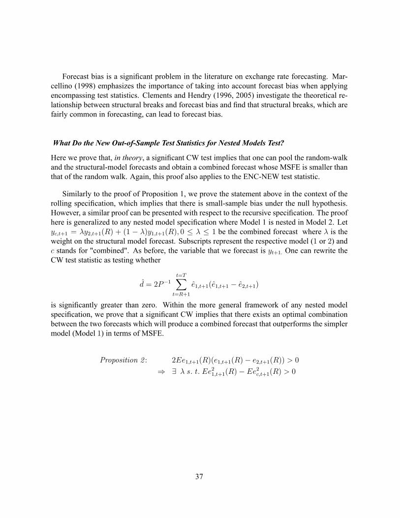
Forecast bias is a signi�cant problem in the literature on exchange rate forecasting. Mar-cellino (1998) emphasizes the importance of taking into account forecast bias when applyingencompassing test statistics. Clements and Hendry (1996, 2005) investigate the theoretical re-lationship between structural breaks and forecast bias and �nd that structural breaks, which arefairly common in forecasting, can lead to forecast bias.

What Do the New Out-of-Sample Test Statistics for Nested Models Test?

Here we prove that, in theory, a signi�cant CW test implies that one can pool the random-walkand the structural-model forecasts and obtain a combined forecast whose MSFE is smaller thanthat of the random walk. Again, this proof also applies to the ENC-NEW test statistic.

Similarly to the proof of Proposition 1, we prove the statement above in the context of therolling speci�cation, which implies that there is small-sample bias under the null hypothesis.However, a similar proof can be presented with respect to the recursive speci�cation. The proofhere is generalized to any nested model speci�cation where Model 1 is nested in Model 2. Letyc;t+1 = �y2;t+1(R) + (1 � �)y1;t+1(R); 0 � � � 1 be the combined forecast where � is theweight on the structural model forecast. Subscripts represent the respective model (1 or 2) andc stands for "combined". As before, the variable that we forecast is yt+1: One can rewrite theCW test statistic as testing whether

d = 2P�1t=TXt=R+1

e1;t+1(e1;t+1 � e2;t+1)

is signi�cantly greater than zero. Within the more general framework of any nested modelspeci�cation, we prove that a signi�cant CW implies that there exists an optimal combinationbetween the two forecasts which will produce a combined forecast that outperforms the simplermodel (Model 1) in terms of MSFE.

Proposition 2 : 2Ee1;t+1(R)(e1;t+1(R)� e2;t+1(R)) > 0) 9 � s : t : Ee21;t+1(R)� Ee2c;t+1(R) > 0

37

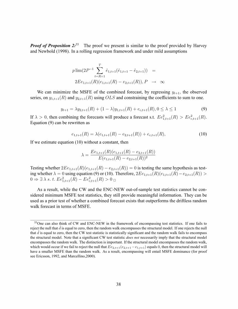
Proof of Proposition 2:55 The proof we present is similar to the proof provided by Harveyand Newbold (1998). In a rolling regression framework and under mild assumptions

p lim(2P�1TX

t=R+1

e1;t+1(e1;t+1 � e2;t+1)) =

2Ee1;t+1(R)(e1;t+1(R)� e2;t+1(R)); P ! 1

We can minimize the MSFE of the combined forecast, by regressing yt+1; the observedseries, on y1;t+1(R) and y2;t+1(R) using OLS and constraining the coef�cients to sum to one.

yt+1 = �y2;t+1(R) + (1� �)y1;t+1(R) + ec;t+1(R); 0 � � � 1 (9)

If � > 0; then combining the forecasts will produce a forecast s.t. Ee21;t+1(R) > Ee2c;t+1(R).Equation (9) can be rewritten as

e1;t+1(R) = �(e1;t+1(R)� e2;t+1(R)) + ec;t+1(R); (10)

If we estimate equation (10) without a constant, then

� =Ee1;t+1(R)(e1;t+1(R)� e2;t+1(R))

E(e1;t+1(R)� e2;t+1(R))2

Testing whether 2Ee1;t+1(R)(e1;t+1(R)� e2;t+1(R)) = 0 is testing the same hypothesis as test-ing whether � = 0 using equation (9) or (10). Therefore, 2Ee1;t+1(R)(e1;t+1(R)�e2;t+1(R)) >0) 9 � s : t : Ee21;t+1(R)� Ee2c;t+1(R) > 0 �

As a result, while the CW and the ENC-NEW out-of-sample test statistics cannot be con-sidered minimum MSFE test statistics, they still provide meaningful information. They can beused as a prior test of whether a combined forecast exists that outperforms the driftless randomwalk forecast in terms of MSFE.

55One can also think of CW and ENC-NEW in the framework of encompassing test statistics. If one fails toreject the null that d is equal to zero, then the random walk encompasses the structural model. If one rejects the nullthat d is equal to zero, then the CW test statistic is statistically signi�cant and the random walk fails to encompassthe structural model. Note that a signi�cant CW test statistic does not necessarily imply that the structural modelencompasses the random walk. The distinction is important. If the structural model encompasses the random walk,which would occur if we fail to reject the null thatEe2;t+1(e2;t+1�e1;t+1) equals 0, then the structural model willhave a smaller MSFE than the random walk. As a result, encompassing will entail MSFE dominance (for proofsee Ericsson, 1992, and Marcellino,2000).

38

C. The Bootstrap

Different Bootstrapping Procedures

First, we brie�y discuss alternative approaches to bootstrapping. The standard bootstrap (alsoknown as "case" bootstrap with replacement), introduced by Efron (1979), assumes that the re-sampled data are independent and identically distributed (iid). If the data are serially correlatedor if heteroskedasticity is present (which is usually the case in time series data), a simple "case"bootstrap leads to inconsistent results. A better way to bootstrap time series data would be viaa block bootstrap which implies that the data is re-sampled in blocks of a certain length ratherthan observation by observation, thereby preserving the properties of the data generating process(DGP). However, �nding the optimal block size to preserve the DGP is not that straight forward.Indeed, Berkowitz and Kilian (1996) suggest that block bootstrapping is not the optimal way tobootstrap time series data given the state of development of the block bootstrap literature.

As a better alternative, Berkowitz and Kilian (1996) suggest a residual bootstrap procedurewhich is the bootstrap speci�cation implemented by Mark (1995) and subsequently improvedby Kilian (1999) and Mark and Sul (2001). The idea of residual bootstrapping is that in spec-i�cations such as Mark (1995) where the independent variable is de�ned as the deviation ofthe exchange rate from the fundamental, the cointegration (or the lack of cointegration) willbe preserved when one uses the residual bootstrap. One way to implement it is to estimate anerror correction speci�cation, then re-sample the estimated residuals and recursively simulatethe independent variable. (This type of bootstrap is commonly referred to as "semi-parametric"bootstrap. If one draws the residuals from a normal distribution, the bootstrap will be called"parametric".) While not always easy to implement, if properly speci�ed, the bootstrap auto-matically corrects for small-sample bias and can be also used for forecast horizons greater thanone as discussed in Kilian (1999).

Bootstrap Used in the Paper

The bootstrap procedure used to calculate the p-values of DMW, TU, CW and ENC-NEW forall speci�cations is similar to the bootstrap of Mark and Sul (2001) and Basher and Westerlund(2006). The main difference between our bootstrap and Mark and Sul's (2001) bootstrap is thatwe use country speci�c OLS - regressions rather than seemingly unrelated regressions (SURs).We also perform a "semi-parametric" rather than "parametric" bootstrap. The data generatingprocess (DGP) is a country � speci�c error correction process. The assumption of no unit root(or cointegration between the fundamental and the exchange rate) is imposed.

For each country, we estimate the following equations using an OLS regression (the �i�subscript is dropped for simplicity) :

39

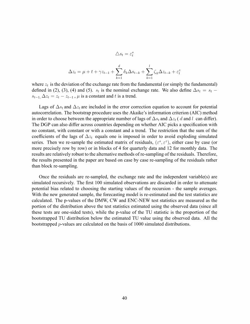
4st = "st

�zt = �+ t+ zt�1 +

dXk=1

�k�st�k +lX

k=1

�k�zt�k + "zt

where zt is the deviation of the exchange rate from the fundamental (or simply the fundamental)de�ned in (2), (3), (4) and (5). st is the nominal exchange rate. We also de�ne �st = st �st�1;�zt = zt � zt�1 , � is a constant and t is a trend.

Lags of �st and �zt are included in the error correction equation to account for potentialautocorrelation. The bootstrap procedure uses the Akaike's information criterion (AIC) methodin order to choose between the appropriate number of lags of�st and�zt ( d and l can differ).The DGP can also differ across countries depending on whether AIC picks a speci�cation withno constant, with constant or with a constant and a trend. The restriction that the sum of thecoef�cients of the lags of �zt equals one is imposed in order to avoid exploding simulatedseries. Then we re-sample the estimated matrix of residuals, ("s; "z), either case by case (ormore precisely row by row) or in blocks of 4 for quarterly data and 12 for monthly data. Theresults are relatively robust to the alternative methods of re-sampling of the residuals. Therefore,the results presented in the paper are based on case by case re-sampling of the residuals ratherthan block re-sampling.

Once the residuals are re-sampled, the exchange rate and the independent variable(s) aresimulated recursively. The �rst 100 simulated observations are discarded in order to attenuatepotential bias related to choosing the starting values of the recursion - the sample averages.With the new generated sample, the forecasting model is re-estimated and the test statistics arecalculated. The p-values of the DMW, CW and ENC-NEW test statistics are measured as theportion of the distribution above the test statistics estimated using the observed data (since allthese tests are one-sided tests), while the p-value of the TU statistic is the proportion of thebootstrapped TU distribution below the estimated TU value using the observed data. All thebootstrapped p-values are calculated on the basis of 1000 simulated distributions.

40