exchange rate regimes, globalisation, and the cost of ... · exchange rate regimes, globalisation,...

Working Paper/Document de travail2007-29

Exchange Rate Regimes, Globalisation, and the Cost of Capital in Emerging Markets

by Antonio Diez de los Rios

www.bankofcanada.ca

Bank of Canada Working Paper 2007-29

April 2007

Exchange Rate Regimes, Globalisation,and the Cost of Capital in

Emerging Markets

by

Antonio Diez de los Rios

Financial Markets DepartmentBank of Canada

Ottawa, Ontario, Canada K1A [email protected]

Bank of Canada working papers are theoretical or empirical works-in-progress on subjects ineconomics and finance. The views expressed in this paper are those of the author.

No responsibility for them should be attributed to the Bank of Canada.

ISSN 1701-9397 © 2007 Bank of Canada

ii

Acknowledgements

This paper is a thoroughly revised and updated version of Chapter II of my Ph.D. dissertation. I

am very grateful to my advisor Enrique Sentana for his guidance and comments. I would also like

to thank Manuel Arellano, José Manuel Campa, Scott Hendry, and Simón Sosvilla for their

comments on earlier versions of this paper. Thanks are also due to Elena Nemykina for her useful

help in collecting the data used in this paper. All remaining errors are mine.

iii

Abstract

This paper presents a multifactor asset pricing model for currency, bond, and stock returns for ten

emerging markets to investigate the effect of the exchange rate regime on the cost of capital and

the integration of emerging financial markets. Since there is evidence that a fixed exchange rate

regime reduces the currency risk premia demanded by foreign investors, the tentative conclusion

is that a fixed exchange rate regime system can help reduce the cost of capital in emerging

markets.

JEL classification: F30, F33, G15Bank classification: Exchange rate regimes; Development economics

Résumé

À l’aide d’un modèle multifactoriel d’évaluation des actifs mettant à contribution les données rel-

atives aux rendements observés sur les marchés de devises, d’obligations et d’actions de dix écon-

omies émergentes, l’auteur analyse l’incidence du choix de régime de change sur le coût du

capital et l’intégration des marchés financiers des économies émergentes. D’après les résultats

qu’il obtient, l’adoption d’un régime de changes fixes entraîne une baisse de la prime de risque de

change exigée par les investisseurs étrangers. La conclusion que l’auteur en tire provisoirement

est qu’un tel régime peut aider à réduire le coût du capital dans les économies émergentes.

Classification JEL : F30, F33, G15Classification de la Banque : Régimes de taux de change; Économie du développement

1 Introduction

In an attempt to reduce the uncertainty that �rms and investors face when making invest-

ment decisions, di¤erent countries have pursued policies oriented to the stabilisation of their

exchange rates. One clear and extreme example of these attempts took place in January 1,

1999, when the conversion rates versus the �Euro�of eleven European countries were irrev-

ocably �xed in order to start the third stage of the European Monetary Union (EMU). It

was claimed at that moment in time that the single currency would provide a new economic

framework where �rms did not need to compensate investors for the exchange rate risk.

This reduction in the cost of capital would, therefore, open new investment opportunities,

stimulate corporate investment and, ultimately, foster investment and growth.

However, as claimed in Sentana (2002), the arguments in favour of a �xed exchange

rate regime su¤er from several criticisms. First, since �rms might be able to hedge their

exchange rate exposure it can be the case that they are not a¤ected by any idiosyncratic

movement in exchange rates. Second, it can be the case that these idiosyncratic exchange

rate risks are not priced in a world with complete market integration. And �nally, a �xed

exchange rate system will increase interest rate volatility since monetary authorities have

to defend their respective parities; and, as long as interest rate volatility might be priced in

emerging markets, it is conceptually possible that a �xed exchange rate regime can increase

the cost of capital. Nevertheless, Sentana (2002) has found that, despite these three points,

the European Monetary System (EMS) has lowered the cost of capital of European �rms,

�although the e¤ect is small�.

At the same time that the �European Experience�went on, policies of exchange rate sta-

bilisation, jointly with those attempting the liberalization of �nancial markets, were blamed

for the increase in the frequency and recurrence of the �nancial upheavals in emerging mar-

kets. This prompts a debate on the appropriate choice of an exchange rate regime for a

developing country (Levy-Yeyati and Sturzenegger, 2003; and Reinhart and Rogo¤, 2004).

For one, emerging markets present several characteristics that can accentuate the bene-

�ts as well as the previously mentioned negative aspects of a �xed exchange rate regime.

External �nancing is relatively more important in emerging countries. For example, the

U.S. holdings of Mexican equities at the end of the year 2001 were approximately 20% of

the domestic market capitalization (Department of the U. S. Treasury, 2003). Therefore,

a reduction of the exchange rate variability could provide a stable framework that stim-

1

ulates foreign investment. On the other hand, Calvo and Reinhart (2002) argue that the

lack of credibility of the exchange rate stabilization policies implemented by the emerging

countries�governments has caused excess volatility in interest rates. This makes the trade-

o¤ between exchange and interest rate volatility to be especially relevant for the study

considered here.

This paper studies the impact of the choice of an exchange rate regime on the cost of

capital in emerging markets. To do so, I rely on the framework of the dynamic version of

the arbitrage pricing theory (APT) developed in King, Sentana and Wadhwani (1994) and

extended in Sentana (2002) to study the impact of EMS on the cost of capital of European

�rms.

In particular, I use weekly data on currency, bond and stock returns for ten emerging

markets over the period from mid 1997 to mid 2006 to estimate a multivariate factor model

with time-varying volatility in the underlying factors. However, I include two modi�cations

to the analysis done in Sentana (2002). First, I do not restrict the structure of the common

factor to be triangular because general equilibrium models usually predict that all common

factors a¤ect all asset classes.1 Second, I follow Jorion (1988), Vlaar and Palm (1993) and

Das (2002) and combine a GARCH speci�cation with the presence of Gaussian jumps. This

allows the model to capture the several episodes of �nancial distress that occur in the sample

(for example, the East Asian crises of 1997, the Russian collapse of 1998, the devaluation

of the Brazilian Real in 1999, and the abandonment of the Argentinean currency board in

2002).

In addition, it is di¢ cult to disentangle the study of the impact of the exchange rate

regime on the cost of capital and the study of the hypothesis of �nancial market integration.

Ultimately, the impact depends on whether country-speci�c risks are priced. The asset-

pricing model used in this paper implicitly assumes that emerging markets are integrated.

Thus, testing the cross-equation restrictions of the basic model allows the paper to answer

if country-speci�c risks are priced. I also follow Stulz (1999) to gauge the potential gains

from stock market globalisation by comparing the risk premia that would prevail in a world

of full integration and full segmentation.

The paper is organized as follows. Section 2 presents the benchmark model and the

estimation procedure. Section 3 reports the empirical results. The impact of an exchange

1See Pavlova and Rigobon (2006) for a general equilibrium model with exchange rates, bond and stockprices.

2

regime on the cost of capital is analysed in section 4. Section 5 discusses whether emerging

markets are �nancially integrated. Finally, section 6 concludes.

2 Benchmark model

This section borrows from Sentana (2002), where further details can be found. However, I

will highlight any signi�cant change with respect to his work.

2.1 Asset pricing model

The analysis is based in a world with a large number of countries j = 1; :::; N , and assumes

that for each country there are three representative assets available: a one-period local

currency (c) deposit with safe gross return Rjcjt; a long-term default-free bond portfolio

(b), which has a random gross holding return over period t in local currency given by Rjbjt;

and a stock portfolio (s), with a random gross holding return in local currency given by

Rjsjt. Let S$jt be the spot exchange rate for country j at the end of period t in terms of the

numeraire currency (US$ in this case), and let R$c$t be the gross return on the safe asset for

US during period t in US$. In this context, the excess returns of these three representative

assets for each country in terms of the numeraire currency will be given by:

r$cjt = logR$cjt � logR$c$t = logS$jt � logS$jt�1 + logRjcjt � logR$c$t;

r$bjt = logR$bjt � logR$c$t;

r$sjt = logR$sjt � logR$c$t;

where r$cjt, r$bjt and r

$sjt are the (continuously compounded) excess returns for currency,

bonds and stocks in US$, respectively. In particular, the notation structure is as follows:

for an excess return r$ajt; the �rst subscript a = c; b; s is related to the asset, the second one

j is related to the country, and the third one t is related to the period of time. Superscript

indicates the currency in which the asset is denominated, and, for clarity of exposition,

it will only appear when the excess return refers to local currency. Thus, the lack of a

superscript re�ects excess returns denominated in US$. In addition, let �ajt and �ajt be

the risk premia term and the unanticipated (as of t � 1) component of the excess returnrajt = �ajt + �ajt. The subscript and the superscript structure for �ajt and �ajt is the same

used for excess returns.

3

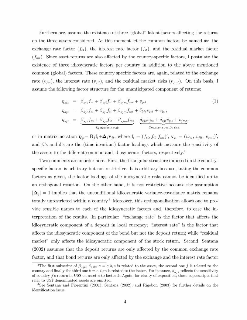
Furthermore, assume the existence of three �global�latent factors a¤ecting the returns

on the three assets considered. At this moment let the common factors be named as: the

exchange rate factor (fet), the interest rate factor (fit), and the residual market factor

(fmt). Since asset returns are also a¤ected by the country-speci�c factors, I postulate the

existence of three idiosyncratic factors per country in addition to the above mentioned

common (global) factors. These country speci�c factors are, again, related to the exchange

rate (vjet), the interest rate (vjit), and the residual market risks (vjmt). On this basis, I

assume the following factor structure for the unanticipated component of returns:

�cjt = �cjefet + �cjifit + �cjmfmt + vjet; (1)

�bjt = �bjefet + �bjifit + �bjmfmt + �bjevjet + vjit;

�sjt = �sjefet + �sjifit + �sjmfmt| {z }Systematic risk

+ �sjevjet + �sjivjit + vjmt| {z };Country-speci�c risk

or in matrix notation �jt= Bjft+�jvjt, where ft = (fet; fit fmt)0, vjt = (vjet, vjit, vjmt)0,

and ��s and ��s are the (time-invariant) factor loadings which measure the sensitivity of

the assets to the di¤erent common and idiosyncratic factors, respectively.2

Two comments are in order here. First, the triangular structure imposed on the country-

speci�c factors is arbitrary but not restrictive. It is arbitrary because, taking the common

factors as given, the factor loadings of the idiosyncratic risks cannot be identi�ed up to

an orthogonal rotation. On the other hand, it is not restrictive because the assumption

j�jj = 1 implies that the unconditional idiosyncratic variance-covariance matrix remainstotally unrestricted within a country.3 Moreover, this orthogonalisation allows one to pro-

vide sensible names to each of the idiosyncratic factors and, therefore, to ease the in-

terpretation of the results. In particular: �exchange rate� is the factor that a¤ects the

idiosyncratic component of a deposit in local currency; �interest rate� is the factor that

a¤ects the idiosyncratic component of the bond but not the deposit return; while �residual

market� only a¤ects the idiosyncratic component of the stock return. Second, Sentana

(2002) assumes that the deposit returns are only a¤ected by the common exchange rate

factor, and that bond returns are only a¤ected by the exchange and the interest rate factor

2The �rst subscript of �ajk, �ajk, a = c; b; s is related to the asset, the second one j is related to thecountry and �nally the third one k = e; i;m is related to the factor. For instance, �ajk re�ects the sensitivityof country j�s return in US$ on asset a to factor k: Again, for clarity of exposition, those superscripts thatrefer to US$ denominated assets are omitted.

3See Sentana and Fiorentini (2001), Sentana (2002), and Rigobon (2003) for further details on theidenti�cation issue.

4

(i.e. �cji = �cjm = �bjm = 0). But given that it is di¢ cult to justify from an empirical and

theoretical point of view that the common (global) factor structure is triangular, I relax

this assumption to provide more �exibility in the structure of covariances of the returns.

Further assumptions are as follows: First, to guarantee that the unanticipated compo-

nent (as of t� 1) of the returns ��s are in fact innovations, the common and speci�c factorsare unpredictable on the basis of past information. Second, the common factors are or-

thogonal to each other, but they have time-varying conditional variances �et, �it, �mt. As a

consequence, the implied risk premia will be time-varying. Third, the idiosyncratic factors,

which by de�nition are orthogonal to ft, are orthogonal to one another for a given country

j, and again, they have time-varying conditional variances !jet, !jit, !jmt. Finally, the

idiosyncratic factors can be correlated across countries, but only mildly to guarantee that

full diversi�cation applies. That is, the conditional covariance matrix has the Chamberlain

and Rothschild (1983) approximate zero-factor structure.

Finally, one can appeal to a no-arbitrage argument to assume that there is a stochastic

discount factor (also known as pricing kernel) that prices the available assets by discounting

their uncertain payo¤s across di¤erent states of the world. In particular, assuming a linear

model in the common factors for the pricing kernel, the risk premia will have the following

beta representation:4

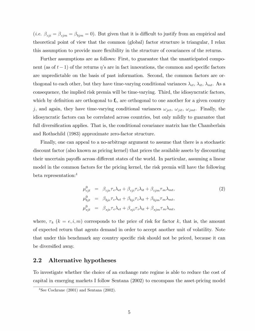
�0cjt = �cje� e�et + �cji� i�it + �cjm�m�mt; (2)

�0bjt = �bje� e�et + �bji� i�it + �bjm�m�mt;

�0sjt = �sje� e�et + �sji� i�it + �sjm�m�mt;

where, � k (k = e; i;m) corresponds to the price of risk for factor k, that is, the amount

of expected return that agents demand in order to accept another unit of volatility. Note

that under this benchmark any country speci�c risk should not be priced, because it can

be diversi�ed away.

2.2 Alternative hypotheses

To investigate whether the choice of an exchange rate regime is able to reduce the cost of

capital in emerging markets I follow Sentana (2002) to encompass the asset-pricing model

4See Cochrane (2001) and Sentana (2002).

5

in a more general set-up:

�cjt = �0cjt + �cje�et + �cji�it + �cjm�mt + �cje!jet; (3)

�bjt = �0bjt + �bje�et + �bji�it + �bjm�mt + �bje!jet + �bji!jit;

�sjt = �0sjt + �sje�et + �sji�it + �sjm�mt + �sje!jet + �sji!jit + �sjm!jmt;

where �0cjt; �0bjt and �

0sjt are de�ned in equation (2).

This system of equations enables one to test several of the hypotheses of interest. First,

one can test whether the exchange rate idiosyncratic risk is priced in bond and stock returns

(�bje = �sje = 0). If this risk is not priced, the choice of an exchange rate regime will have

no impact on the currency component of the cost of capital. Second, if the interest rate

idiosyncratic risk is priced in bond and stock returns (�bji 6= 0 or �sji 6= 0) then the choiceof an exchange rate regime can a¤ect the cost of capital when there is an increase in the

interest rate volatility caused by the defense of a �xed exchange rate regime. Third, it is

also possible that other sources of idiosyncratic risk are priced in stocks (�sjm 6= 0) whichwould reveal that emerging markets are not fully integrated. Finally, I investigate whether

the prices of risk are common across countries (�ajk = 0 8a = c; b; s 8k = e; i;m).

2.3 Estimation method

Given that rajt = �ajt + �ajt by construction, I combine the system of equations (1) and

(2) to write the model in compact form as:

rcjt = �cjefRet + �cjif

Rit + �cjmf

Rmt + vjet; (4)

rbjt = �bjefRet + �bjif

Rit + �bjmf

Rmt + �bjevjet + vjit;

rsjt = �sjefRet + �sjif

Rit + �sjmf

Rmt + �sjevjet + �sjivjit + vjmt;

or in matrix notation rjt= BjfRt +�jvjt. Here fRkt = � k�kt + fkt = �kt + fkt (k = e; i;m)

can be interpreted as excess returns of three diversi�ed portfolios, fRt = (fRet ; f

Rit ; f

Rmt)

0, that

mimic the proposed factors. In particular, �kt represents the risk premia of the common

factor k and fkt is the corresponding unanticipated component (as of t� 1).Note that if fRt were observed directly, estimation would be an easy task since one would

be able (in the conditional homoscedastic case) to recover Bj and �j by a set of OLS

regressions.5 In this particular case where fRt is observed and conditionally homoscedastic,

5Alternatively, under the assumption of conditional normality, the system given by (4) could be es-

6

the structure of the problem allows the estimation of Bj and �j by maximum likelihood

(ML) simply as follows (see Sentana 2002 and references therein):

(a) �cje; �cji; �cjm and !je from the OLS regression of rcjt on fRet , fRit and f

Rmt:

(b) �bje; �bji; �bjm; �bje and !ji from the OLS regression of rbjt on fRet , fRit and f

Rmt with

the residual from (a) as an extra regressor.

(c) �sje; �sji; �sjm; �sje; �sji and !jm from the OLS regression of rsjt on fRet , fRit and f

Rmt

with the residuals from (a) and (b) as extra regressors.

However, this is not the case because there is no data available on fRt . Still, I follow

Sentana (2002) and construct three fully diversi�ed global portfolios of currency deposits,

bonds and stocks which by de�nition do not contain any idiosyncratic risk. Let the excess

returns on these three portfolios be denoted by rpt = (rcpt; rbpt; rspt)0 and assume that they

are related to the common risk factors in the following way:

rcpt = fRet ; (5)

rbpt = �bpefRet + fRit ;

rspt = �spefRet + �spif

Rit + fRmt;

or in matrix notation rpt = BpfRt , where the scaling of the common factors are set to

�cpe = �bpi = �spm = 1.6

Now, I can estimate Bp, recover the set of mimicking portfolios as bfRt = bB�1p rpt andrun the OLS regressions in (a), (b) and (c) with bfRt = ( bfRet ; bfRit ; bfRmt) instead of fRt . In otherwords, adding the three portfolios in (5) to the list of 3N assets allows the factorisation of

the joint likelihood function of the 3(N +1) assets into the marginal component of rpt and

the conditional components corresponding to all the individual countries given the fully

timated for any N countries simultaneously by maximum likelihood (see King, Sentana and Wadhwani,1994). But as claimed in Sentana (2002): �with three assets per country and a non-diagonal time-varyingconditional idiosyncratic covariance matrix, though, this results in a very time-consuming procedure evenfor moderately large N�.

6As in the case of the idiosyncratic factors, the triangular structure imposed on the diversi�ed portfoliosis arbitrary but not restrictive. Again, the factor loadings of the three diversi�ed portfolios to the commonrisks cannot be identi�ed up to an orthogonal rotation and therefore we can always rede�ne the diversi�edportfolios and get the same covariance structure. Nevertheless, under a di¤erent orthogonalisation it wouldbe di¢ cult to understand these common factors as �exchange rate�, �interest rate�and �residual market�.Moreover, it is important to note that this speci�cation is not restrictive because, given the assumptionjBpj = 1, the unconditional variance-covariance matrix of the global portfolios remains totally unrestricted.

7

diversi�ed portfolios. In particular, under conditional homoskedasticity, (5) is a recursive

simultaneous equation system whose parameter estimates can be obtained in the following

way:

(d) �e and �e from the OLS regression of rcpt on a constant.

(e) �bpe; �i and �i from the OLS regression of rbpt on rcpt and a constant.

(f) �spe; �spi; �m and �m from the OLS regression of rspt on rcpt; (rbpt � b�bpercpt) and aconstant, where b�bpe is the estimation of the parameter �bpe obtained in (e).

Therefore, one would estimate the system of the diversi�ed portfolios (5) in a �rst

stage, and then estimate the corresponding system for the individual countries in (4) in a

second step. But given that I am using estimates of the diversi�ed portfolios system to

compute the regressors of the second stage, the inference will not be valid because it su¤ers

from a �generated regressors problem�. This is solved by estimating the joint system and

recasting the estimation within the Generalized Method of Moment (GMM) framework

using the moment conditions that are implicit in the OLS estimation in (a)�(f). Moreover,

a signi�cant advantage of the GMM framework is that estimates of ��s, ��s and ��s remain

consistent when factors su¤er from serial correlation and/or are a¤ected by conditional

heteroscedasticity, provided that the factor representing portfolios and idiosyncratic factors

remain contemporaneously uncorrelated.

Similarly, the alternative hypotheses stated in section 2.2 can also be tested within the

GMM-regression framework. For example, I can add the conditional variance of vjet, !jet

as an additional regressor in equation (4a) and test whether the estimated coe¢ cient �cjeis di¤erent from zero. Doing so yields an estimate of �cje which measures the impact of the

elimination of idiosyncratic exchange rate volatility.

In practice, the conditional variance is an unobserved variable and, instead, one has to

use an estimate b!jet. Although I could follow Sentana (2002) to estimate volatilities bymeans of GARCH (1,1) regressions, this model fails in replicating the episodes of �nancial

distress that characterize emerging market returns. Consequently, I follow instead Jorion

(1988), Vlaar and Palm (1993) and Das (2002) to combine a GARCH speci�cation with

the presence of Gaussian jumps. The estimation of these GARCH-jump models is done

by replacing the OLS regressions in (a)�(c) by GARCH-jump regressions, and replacing

8

the OLS regressions in (d)�(f) by GARCH-in-mean-jump regressions.7 Moreover, if the

proposed conditional variance speci�cation were incorrect, the tests would still be consistent

albeit less powerful. In addition, the tests will have the correct asymptotic size under the

null hypothesis despite the fact that conditional variances are generated regressors.8

3 Results

3.1 Data

The database comprises weekly data for currency, bond and stock returns on a set of ten

emerging markets during the period 4 June 1997 - 28 June 2006 (474 observations). It in-

cludes four Latin-American countries: Argentina, Brazil, Mexico, and Venezuela; four Asian

markets: China, Malaysia, Philippines, and Thailand; and two East European economies:

Poland, and Russia. This set of countries has been chosen on a data-availability basis. An

appendix with data sources is provided.

I also include data on developed countries to aggregate well-diversi�ed portfolios that

contain the non-emerging markets as well. These are Australia, Canada, Japan, the United

States and ten European countries (Belgium, Denmark, France, Germany, Italy, Nether-

lands, Spain, Sweden, Switzerland and the United Kingdom). In particular, these data are

used to construct three equally weighted portfolios: a �world�equally weighted portfolio

of currency returns, a �world�equally weighted portfolio of bond returns, and a �world�

equally weighted portfolio of stock returns as the set of portfolios in system (5).

3.2 Estimates of the baseline asset pricing model

I �rst estimate the baseline model of section 2 by GMM under the null hypothesis of

integration of �nancial markets. In order to obtain estimates of the conditional variances, I

then �t a GARCH-in-mean-jump model to the common factors estimated in the �rst step,

and a GARCH-jump model to the estimated idiosyncratic factors.

The parameter estimates of the diversi�ed portfolios subsystem, equation (5), are pre-

sented in Table 1. These results indicate that the three diversi�ed portfolios are positively

correlated, which is partly explained by the fact that all returns are denominated in US$.

The parameter estimates also con�rm the result found in Sentana (2002) that, controlling

7See the appendix for the speci�c details of the likelihood function of GARCH-jump models.8See Sentana (2002) for details on these two last issues.

9

for movements in exchange rates, world bond returns and world stock returns are positively

correlated. While the estimated risk premia on the interest rate and residual market are

positive, the exchange rate risk premia is negative. However, none of the three risk premia

is estimated precisely. The interest rate risk premia is signi�cant, though, but only at the

ten percent level.9

Table 2 reports the estimates of the factor loadings of currency deposit, bond and stock

returns on each one of the factors. In particular, the parameter estimates of the sensitivities

of the currency deposit returns to the three common risk factors are presented in the Table

2a. In the �rst column, I �nd that the coe¢ cient on the common exchange rate factor, �cje,

is positive for the ten countries analyzed in this paper and this coe¢ cient is signi�cant10

for eight out of the ten countries. Since the common link across all the exchange rates is

the numeraire currency, these positive coe¢ cients suggest that currency returns decrease

(increase) when the dollar appreciates (depreciates). In the second column, one can see

that the currency deposit return of Mexico and Poland are positively correlated with the

�world�portfolio of bond returns, while the currency deposits in Malaysia are negatively

correlated. For the rest of the countries, �cji is not statistically di¤erent from zero. Finally,

in the third column, all the countries have a coe¢ cient �cjm that is positive. Still, only

Argentina, Brazil, Mexico, Philippines, Thailand and Poland present a positive coe¢ cient

that is statistically di¤erent from zero.

While the sensitivities of currency deposit returns to the risk factors correspond to

assets denominated in US$, the parameter estimates in table 2b and 2c correspond to bond

and stock returns denominated in local currency. This way, one can isolate any indirect

e¤ect of exchange rates onto asset returns. Moreover, the analysis presented in the previous

section is still valid because the asset pricing model considers currency deposit returns and,

therefore, the framework presented in section 2.1 can also be used to price bond and stock

returns in local currency. Speci�cally, note that local currency bond and stock excess

returns can be expressed as rjbjt = rbjt � rcjt and rjsjt = rsjt � rcjt. Making use of these

expressions and those in (4) I can write:

rjbjt = (�bje � �cje)fRet + (�bji � �cji)f

Rit + (�bjm � �cjm)f

Rmt + (�bje � 1)vjet + vjit

= �jbjefRet + �jbjif

Rit + �jbjmf

Rmt + �jbjevjet + vjit; (6)

9The price of risk coe¢ cients obtained from the GARCH-in-mean-jump model are �e = 0:0119, � i =0:1938, and �e = 0:0171.10From now on, I consider tests at the 5% level of signi�cance.

10

and similarly:

rjsjt = (�sje � �cje)fRet + (�sji � �cji)f

Rit + (�sjm � �cjm)f

Rmt (7)

+(�sje � 1)vjet + �sjivjit + vjmt

= �jsjefRet + �jsjif

Rit + �jsjmf

Rmt + �jsjevjet + �sjivjit + vjmt:

Table 2b presents the estimates of the factor loadings of local currency bond returns

on each one of the common factors as well as those parameters related to the country-

speci�c exchange rate risk. In the �rst column, I �nd that the coe¢ cient on the common

exchange rate factor, �jbje, is positive and signi�cant only in China. As in the case of

currency returns, this �nding implies that local currency bond returns decrease (increase)

when the dollar appreciates (depreciates). On the other hand, the negative and signi�cant

coe¢ cient found in Thailand and Poland implies that the local currency bond returns in

these two countries decrease when the dollar depreciates. In the second column, I �nd that

bond returns are all positively correlated through the common interest rate factor. The

coe¢ cient �jbji is positive and statistically di¤erent from zero for all the countries. In the

third column, the estimates of the factor loadings on the common residual market risk are

signi�cantly positive for Brazil, Venezuela, the Philippines and Russia. On the other hand,

this coe¢ cient is statistically negative for China and Poland. Note that the sensitivity of

Chinese bond returns to common exchange rate movements is positive, while its sensitivity

to idiosyncratic exchange rate movements is negative. As claimed in Sentana (2002), this

di¤erence in the sensitivity to common and idiosyncratic exchange rate risk is likely to

re�ect the structure of its foreign trade. Finally the fourth column reports the estimates of

the factor loadings of bond returns on the idiosyncratic exchange rate factor, �jbje. Here, the

predominant sign is the negative one. In addition, all coe¢ cients are statistically di¤erent

from zero. Since the idiosyncratic exchange rate factor is the residual of the regression of the

currency return on the three common factors, these negative coe¢ cients imply that, taking

the common factors as given, bond returns fall (rise) when the local currency appreciates

(depreciates).

Table 2c reports the estimates of the factor loadings of local currency stock returns. In

the �rst column, I �nd that the coe¢ cient on the common exchange rate factor, �jsje, is

positive and signi�cant for Brazil and the Philippines. In the second column, the estimates

of the factor loadings on the common interest rate factor, �jsji, are all positive and the

coe¢ cient is statistically signi�cant for Argentina, Brazil, Mexico, Venezuela and Russia. In

11

the third column, I �nd that all the coe¢ cients on the common residual market factor, �jsjm,

are positive and statistically di¤erents from zero. The fourth column presents the estimates

of the factor loadings of stock returns to the idiosyncratic exchange rate factor, �jsje. These

are statistically negative for Argentina, Venezuela and Russia. Thus, stock returns for these

countries tend to fall (rise) when the local currency appreciates (depreciates). On the other

hand, �jsje is statistically positive for the Philippines. Finally, the �fth column reports the

estimates of the factor loadings of stock returns on the idiosyncratic interest rate factor,

�jsji. Since these coe¢ cients are positive with the exception of Poland (although, again,

the coe¢ cient is not signi�cant), stock and bond returns seem to be positively correlated

within a country.

4 Direct e¤ects of the exchange rate regime on thecost of capital

A (credible) �xed exchange rate regime reduces the uncertainty induced by currency move-

ments. Since the elimination of the exchange rate risk would reduce the risk premium,

this reduction in the cost of capital will open new investment opportunities and will spur

growth. However, there are several reasons these arguments might break down. For exam-

ple, exchange rate risk may not be priced. Second, the monetary authority has to defend

the level of the currency with the consequent increase of the interest rate volatility. If

interest rate risk is also priced in stock returns, the increase of the interest rate risk can

o¤set the gain obtained by the elimination of the exchange rate uncertainty.

Therefore, is the cost of capital lower in those countries that have adopted a �xed ex-

change rate regime? To address this question, I use a �de facto�classi�cation of exchange

rate regimes proposed by Levy-Yeyati and Sturzenegger (2003) (LYS from now on) to group

the countries into those that have followed a �xed exchange rate system, and those that

followed a �oating one. In particular, and in line with these two authors, I expect this clas-

si�cation to provide a better characterization of the exchange rate policies, regardless of the

regime reported by the country�s authorities and published �de jure�by the International

Monetary Fund. Following the LYS classi�cation, I include Argentina, Brazil, Venezuela,

China and Malaysia in the �xed exchange rate regime block; and Mexico, the Philippines,

Thailand and Poland in the �oating one. Russia has been dropped because its exchange

rate regime has changed many times during the period of the study.

12

Figure 1a displays the average of the (estimated) conditional standard deviation of the

idiosyncratic exchange rate factor. The e¤ect of the emerging markets crises is clear in

the conditional volatility of the countries with �xed exchange rate regimes. There is no

noticeable change in the magnitude of the movements of the volatility of those countries

with a �exible exchange rate regime. In fact, the continual realignments of the currency peg

(as in the case of Venezuela) or even its abandonment (Argentina and Brazil) has caused the

level of the (idiosyncratic) volatility to be substantially larger for those countries that have

�xed their exchange rates. Therefore, their exchange rate stabilisation polices have been

unsuccessful. Equally important, Figure 1b presents the (estimated) conditional standard

deviation of the idiosyncratic interest rate factor. The ranking is the same. The e¤ect of

�nancial turbulence is noticeable in both groups of countries, although it is more noticeable

for those countries with a �xed exchange rate system. This means that not only has a

�xed exchange rate regime been unable to reduce the exchange rate volatility in emerging

markets, but it has also increased the interest rate volatility. This result is related to Calvo

and Reinhart (2002). The lack of credibility of the �xed exchange rate regime has caused

excess volatility in interest rates.

Still, the (idiosyncratic) movements should not be priced under the hypothesis of �nan-

cial integration (see next section for more details). For this reason, I continue by testing

whether, contrary to the theory, idiosyncratic exchange rate and interest rate risks are

priced. Table 3 reports the tests on the pricing of country-speci�c volatility. The main

results are the following. First, the exchange rate risk is priced in currency deposit returns

for those countries with a �exible exchange rate regime. That is, the idiosyncratic exchange

rate factor is more volatile for those countries with a �xed exchange rate regime (see Figure

1a), but it is not priced. Second, the exchange rate risk is priced in stock returns for those

countries with a �xed exchange rate regime which implies that stock market investors de-

mand compensation for the risk of a currency devaluation. Third, the interest rate risk is

priced in (local currency) bond returns in those countries with a �xed exchange rate regime.

Bond investors demand compensation for the excess volatility in interest rate caused by

the defense of the level of the currency.

The analysis of the estimated sensitivities to the idiosyncratic risk factors, �ajk for

a = c; b; s and k = e; i, should give a good measure of the impact of the elimination of

these country-speci�c risks. However, there are some problems with this approach. First,

13

these (estimated) coe¢ cients show great dispersion, being sometimes negative. Second and

more important, the e¤ects of idiosyncratic exchange rate and interest rate volatility may

compensate each other. Therefore, I follow Sentana (2002) and measure the net e¤ect of

idiosyncratic exchange rate and interest rate movements on each asset by computing the

di¤erences in �tted values between the alternative and null hypothesis. This procedure has

the advantage that each country acts as its own control.

The average net e¤ect of idiosyncratic exchange rate volatility on currency returns across

countries with a �xed and �exible exchange rate regime is presented in Figure 2a. Figures

2b and 2c present the analogous net e¤ect of idiosyncratic exchange rate and interest rate

risks on bond and stocks returns, respectively. Furthermore, sample means and relevant

Wald tests (robust to serial correlation and conditional heteroskedasticity) are reported in

Table 4. Figure 2a shows that the net e¤ect of idiosyncratic exchange rate volatility on

currency returns is more important in those countries with a �exible exchange rate regime.

In fact the di¤erence between the e¤ect in countries with a �oating and a �xed exchange

rate regime is positive most of the time. As shown in Table 4, this di¤erence is signi�cant at

the 10% level. Figure 2b shows a similar picture. The net e¤ect of idiosyncratic exchange

rate and interest rate volatility on bond returns seems to be more important in those

countries with a �exible exchange rate regime. However, the di¤erence is not statistically

di¤erent from zero. Finally, the analysis of Figure 2c suggests that there is no clear e¤ect

of the exchange rate regime on (local currency) stock returns: the increase in the interest

rate volatility seem to o¤set the decrease in the volatility of the idiosyncratic exchange

rate factor. Therefore, since there is evidence that a �xed exchange rate regime reduces

the currency risk premia demanded by foreign (U.S.) investors and foreign investment is

an important source of emerging market �nancing, the tentative conclusion is that a �xed

exchange rate regime system can help reduce the cost of capital of emerging market �rms.

5 Integration of emerging �nancial markets

The hypothesis of market integration plays a central role in emerging market �nance be-

cause it helps to identify the bene�ts of the process of liberalization that many emerging

markets have followed. In particular, economic theory predicts that the process of �nancial

liberalization will reduce the cost of capital (see Errunza and Losq, 1985). In this section, I

retake the tests of pricing of idiosyncratic risks to analyze whether the hypothesis of market

14

integration is valid in emerging �nancial markets.

The de�nition of international �nancial integration implies that assets with identical

risk should command the same expected return regardless of their nationality. This means

that no country-speci�c risk should be rewarded in a world of complete integration (�ajk = 0

8a = c; b; s 8k = e; i;m); and, secondly, the price of (common) risk should be equal across

countries (�ajk = 0;8a = c; b; s 8k = e; i;m). In section 4, I have examined whether

idiosyncratic exchange and interest rate factors are priced for countries with a �xed and

�exible exchange rate system as an exercise to analyze the impact of an exchange rate

regime. Now, I repeat the analysis taking into account regional blocks, that is Latin

America, Asia and East Europe, rather than exchange rate systems. I also include a test

for the pricing of country-speci�c residual market risk and tests for the equality of the

prices of common risks.

Table 5a reports the additional tests of market integration on the pricing of idiosyncratic

risks. The �ndings are the following: First, the exchange rate risk is priced in the currency

and stock returns of Latin America and Eastern Europe. It is only priced in bond returns

of Eastern Europe. Second, the idiosyncratic interest rate risk is priced in the Asian bond

returns at the ten percent level of signi�cance. Finally, the idiosyncratic residual market

risk is not priced in the equity market. On the other hand, Table 5b presents the tests for

the equality of common risk prices. The analysis of this table suggests that prices of the

(global) exchange rate, the interest rate and the residual market risks seem to be di¤erent in

currency returns of Asia and Eastern Europe. The prices of the (global) exchange rate, the

interest rate and the residual market risks are equal for bond and stock returns. Overall,

the bond and stock markets seem to be integrated, while the currency market does not.

5.1 Globalisation and the cost of capital

Finally, I follow Stulz (1999) to measure the potential gains from the globalisation process

by comparing the stock market risk premia under full integration with the risk premia

that would prevail in the context of fully segmented markets. In particular, note that it is

possible to decompose the unanticipated components of stock returns into three orthogonal

components:

�jsjt = �jsjefet + �jsje| {z } + �jsjifit + �sji| {z } + �jsjmfmt + �sjm| {z } :Exchange rate risk Interest rate risk Residual market risk

15

Since the stock portfolio for each country corresponds to a well-diversi�ed basket of

domestic stocks one can obtain the risk premia that would prevail in this context using a

domestic argument similar to the one presented in Section 2. In particular, this will result

in the risk premia corresponding to a domestic APT pricing relationship:

�jssjt = 'je�(�jsje)

2�et + (�jsje)

2!jet�+

+'ji�(�jsji)

2�it + �2sji!jit�+ 'jm

�(�jsjm)

2�mt + �2sjm!jmt�;

where 'jk is the price of risk for country j and factor k = e; i;m in a fully segmented market

framework. Assuming that all investors in the world have the same constant relative risk

aversion, and that the price of the residual market risk and the statistical properties of

asset returns are not a¤ected by the globalisation process, I can compare the following risk

premia:

Risk premia under full integration = �m�jsjm�mt; (8)

Risk premia under full segmentation = 'jm�(�jsjm)

2�mt + �2sjm!jmt�: (9)

Subsequently, I can assess whether there would be gains from a process of stock market

integration, for each country comparing:

�sjmE [�mt] 7 �2sjmE [�mt] + �2sjmE [!jmt] :

The (estimated) di¤erences between both sides of the above expression for each one

of the emerging countries in the database are displayed in Table 6. Its analysis reveals

ample evidence in favour of globalisation gains because these di¤erences are all positive

and signi�cantly di¤erent from zero. Furthermore, there is an important variation across

countries, where Russia is the country with the largest average, followed by China and

Thailand. Moreover, if one multiplies these di¤erences by 0.017, which is the estimate of

�m, these results suggest that the globalisation gains can be rather large for these countries.

On the other side, Mexico and Brazil are the countries with the smallest estimated gains.

These two countries have signi�cantly smaller idiosyncratic residual market risk variance

(see Table 2c), and this suggests that they already have closer links with world markets.

Finally, it is very important to emphasize that these gains should only be taken as indicative

given that I am comparing two extreme situations.

16

6 Concluding remarks

In this article I attempt to shed some light on two important questions in international

�nance: whether the choice of a �xed exchange rate regime is able to reduce the cost of

capital and whether there are gains from the process of globalisation. For that reason, this

paper presents a multifactor asset-pricing model that is estimated using weekly data on

currency, bond and stock returns for ten emerging markets over the period from 4 June

1997 to 28 June 2006.

The �ndings in this paper suggest that not only has a �xed exchange rate regime been

unable to reduce the exchange rate volatility in emerging markets, but it has also increased

the interest rate volatility. This result is related to Calvo and Reinhart (2002). The lack of

credibility of the �xed exchange rate regime has caused excess volatility in interest rates.

However, there is evidence that a �xed exchange rate regime reduces the currency risk

premia demanded by foreign investors. Therefore, the tentative conclusion is that a �xed

exchange rate regime system can help reduce the cost of capital in emerging markets. In

addition, the evidence against the hypothesis of integration of �nancial markets is mixed

and depends on the market under examination. At the same time, I cannot reject the null

hypothesis of the integration of emerging equity markets. A comparison between the risk

premia that would prevail in a world of full integration and full segmentation reveals rather

large gains from the process of liberalization of stock markets in some countries.

17

Appendix

A Database description

Details of the data series used are as follows.Short interest rates:- Belgium, Denmark, France, Germany, Italy, Netherlands, Spain, Sweden, Switzerland,

UK; Canada, Japan; Thailand: Euro-local currency 1 week.- Argentina: Interbank 7 days - middle rate.- Australia: Deposit 1 week.- China: Demand deposit rate - middle rate.- Brazil: CDI - Middle Rate.- Malaysia, Poland: Interbank 1 week - middle rate.- Mexico: Balance (TIIE) interbank rate.- Philippines: Interbank call loan rate - middle rate.- Russia: Interbank 2 to 7 days - middle rate.- Venezuela: Overnight - middle rateBond returns:- Belgium, Denmark, France, Germany, Italy, Netherlands, Spain, Sweden, Switzerland,

UK; USA, Canada, Japan, Australia: Morgan Stanley Capital International Total ReturnIndex (in local currency).- Argentina, Brazil, Mexico, Venezuela; China, Malaysia, Philippines, Thailand; Poland,

and Russia: J.P. Morgan EMBI Global Index (in U.S. dollars)Stock prices:- All countries: Morgan Stanley Capital International Return Index (in U.S. dollars)

B Likelihood function of the GARCH-jump regres-sion model

In this appendix, I provide the details of the likelihood function of the GARCH-jumpregression model. As in Ball and Torous (1983), jumps are modeled by a mixture oftwo normal distributions where one state represents periods of calm, and the other onerepresents the state where a jump has occurred.Assume that a stationary time series of returns yt (t = 1; : : : T ) is observed and assume

the following regression model:yt = x

0t� + "t; (10)

where x0t denotes a vector of predetermined explanatory variables (i.e. the returns of thefactor representing portfolios fRt ). The disturbance term "t is assumed to satisfy, conditional

18

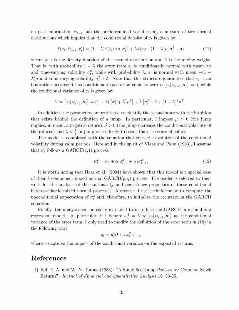
on past information t�1 and the predetermined variables x0t, a mixture of two normal

distributions which implies that the conditional density of "t is given by:

f("tj t�1;x0t) = (1� �)�("t;��; �2t ) + ��("t;�(1� �)�; �2t + �); (11)

where �(�) is the density function of the normal distribution and � is the mixing weight.That is, with probability 1 � � the error term "t is conditionally normal with mean ��and time-varying volatility �2t ; while with probability �, "t is normal with mean �(1 ��)� and time-varying volatility �2t + �. Note that this structure guarantees that "t is aninnovation because it has conditional expectation equal to zero E

�"tj t�1;x0t

�= 0, while

the conditional variance of "t is given by:

V ar�"tj t�1;x0t

�= (1� �)

��2t + �2�2

�+ �

��2t + � + (1� �)2�2

�:

In addition, the parameters are restricted to identify the second state with the intuitionthat exists behind the de�nition of a jump. In particular, I impose � > 0 (the jumpimplies, in mean, a negative return), � > 0 (the jump increases the conditional volatility ofthe returns) and � < 1

2(a jump is less likely to occur than the state of calm).

The model is completed with the equation that rules the evolution of the conditionalvolatility during calm periods. Here and in the spirit of Vlaar and Palm (1993), I assumethat �2t follows a GARCH(1,1) process:

�2t = �0 + �1"2t�1 + �2�

2t�1: (12)

It is worth noting that Haas et al. (2004) have shown that this model is a special caseof their k-component mixed normal GARCH(p; q) process. The reader is referred to theirwork for the analysis of the stationarity and persistence properties of these conditionalheteroskedastic mixed normal processes. Moreover, I use their formulae to compute theunconditional expectation of �2t and, therefore, to initialize the recursion in the GARCHequation.Finally, the analysis can be easily extended to introduce the GARCH-in-mean-Jump

regression model. In particular, if I denote !2t = V ar�"tj t�1;x0t

�as the conditional

variance of the error term, I only need to modify the de�nition of the error term in (10) inthe following way:

yt = x0t� + �!2t + "t;

where � captures the impact of the conditional variance on the expected returns.

References

[1] Ball, C.A. and W. N. Torous (1983): �A Simpli�ed Jump Process for Common StockReturns�, Journal of Financial and Quantitative Analysis 18, 53-65.

19

[2] Bollerslev, T. and J. M. Wooldridge (1992): �Quasi-Maximum Likelihood Estima-tion and Inference in Dynamic Models with Time-Varying Variances�, EconometricReviews, 11, 143-72.

[3] Calvo, G. and C. M. Reinhart (2002): �Fear of Floating�, Quarterly Journal of Eco-nomics, 117, 2, 379-408.

[4] Chamberlain, G. and M. Rothschild (1983): �Arbitrage, Factor Structure, and Mean-Variance Analysis on Large Asset Markets�, Econometrica, 51, 1281-304.

[5] Cochrane, J.H. (2001): Asset Pricing. Princeton, Princeton University Press.

[6] Das, S. R. (2002): �The Surprise Element: Jumps in Interest Rates�, Journal ofEconometrics, 106, 27-65.

[7] Department of the Treasury (2003): Report on U.S. Holdings of Foreign Securities

[8] Errunza, V. and E. Losq (1985): �International Asset Pricing under Mild Segmenta-tion: Theory and Test�, Journal of Finance, 40, 105-124.

[9] Haas M., S. Mittnik and M.S. Paolella (2004): �Mixed Normal Conditional Het-eroskedasticity�, Journal of Financial Econometrics, 2, 211-250.

[10] Jorion, P. (1988): �On Jump Processes in the Foreign Exchange and Stock Markets�,Review of Financial Studies, 1,4, 427-445.

[11] King, M., E. Sentana and S. Wadhwani (1994): �Volatility and Links Between NationalStock Markets�, Econometrica, 62,4, 901-933.

[12] Levy-Yeyati, E. and F. Sturzenegger (2003): �To Float or to Trail: Evidence on theImpact of Exchange Rate Regimes�, American Economic Review, 93, 1173-93.

[13] Newey, W. and K.D. West (1987): �A Simple Positive Semi-De�nite Heteroskedasticityand Autocorrelation Consistent Covariance Matrix�, Econometrica 55, 703-6.

[14] Pavlova, A. and R. Rigobon (2006): �Asset Prices and Exchange Rates�, forthcomingReview of Financial Studies.

[15] Reinhart, C. M. and K. S. Rogo¤ (2004): �The Modern History of Exchange RateArrangements: A Reinterpretation�, Quarterly Journal of Economics, 119, 1-48.

[16] Rigobon, R. (2003): �Identi�cation Through Heteroskedasticity�, Review of Eco-nomics and Statistics, 85, 777-792.

[17] Sentana, E. (2002): �Did the EMS Reduce the Cost of Capital?�, Economic Journal,112, 786-809.

20

[18] Sentana, E. and G. Fiorentini (2001): �Identi�cation, Estimation and Testing of Con-ditionally Heteroskedastic Factor Models�, Journal of Econometrics, 102, 143-164.

[19] Stulz, R. (1999): �Globalization of Equity Markets and the Cost of Capital�, DiceCenter WP 99-1, Ohio State University.

[20] Vlaar, P.J.G and F.C. Palm (1993): �The Message in Weekly Exchange Rates in theEuropean Monetary System: Mean Reversion, Conditional Heteroskedasticity, andJumps�, Journal of Business and Economic Statistics 11, 351-60.

21

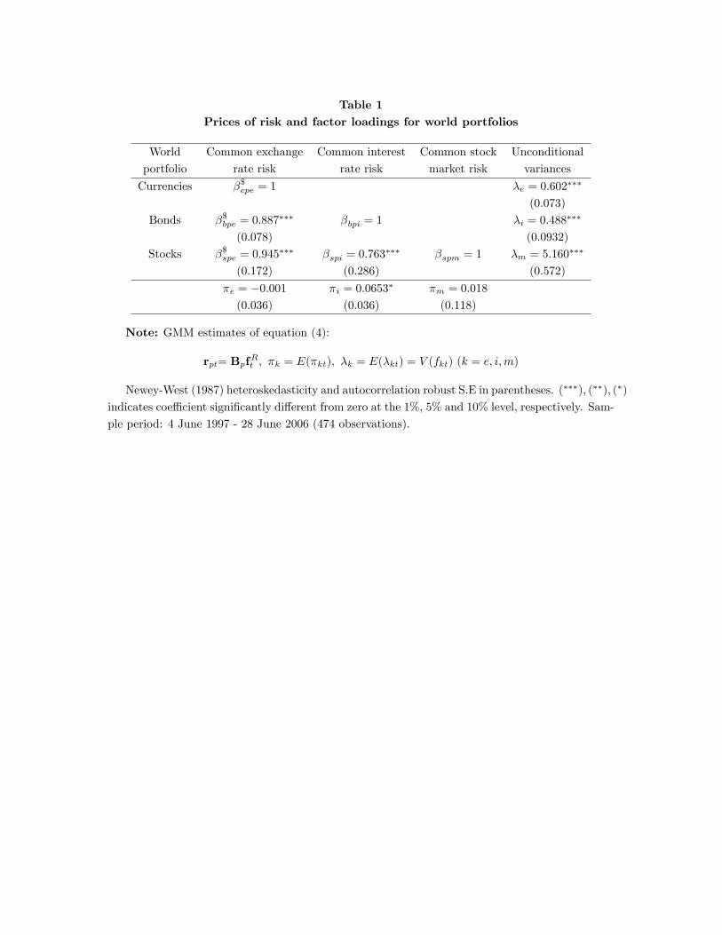
Table 1Prices of risk and factor loadings for world portfolios

World Common exchange Common interest Common stock Unconditional

portfolio rate risk rate risk market risk variances

Currencies �$cpe = 1 �e = 0:602��

(0:073)

Bonds �$bpe = 0:887�� bpi = 1 �i = 0:488

��

(0:078) (0:0932)

Stocks �$spe = 0:945�� spi = 0:763

�� spm = 1 �m = 5:160��

(0:172) (0:286) (0:572)

�e = �0:001 �i = 0:0653� �m = 0:018

(0:036) (0:036) (0:118)

Note: GMM estimates of equation (4):

rpt= BpfRt ; �k = E(�kt); �k = E(�kt) = V (fkt) (k = e; i;m)

Newey-West (1987) heteroskedasticity and autocorrelation robust S.E in parentheses. (��); (��); (�)

indicates coe¢ cient signi�cantly di¤erent from zero at the 1%, 5% and 10% level, respectively. Sam-

ple period: 4 June 1997 - 28 June 2006 (474 observations).

Table 2aFactor loadings for currency returns ($)

Country Common Common Common Idiosyncratic

exch. rate int. rate market variance

risk (�cje) risk(�cji) risk (�cjm) (!je)

Argentina 0.674 -0.657 0.130�� 9.102�

(0.428) (0.508) (0.063) (5.193)

Brazil 0.922�� 0.067 0.258�� 6.652��

(0.271) (0.225) (0.087) (2.021)

Mexico 0.239�� 0.402�� 0.188�� 1.156��

(0.106) (0.134) (0.027) (0.127)

Venezuela 0.681�� -0.820� 0.079 12.404��

(0.237) (0.433) (0.049) (4.947)

China 0.012�� -0.008 0.002 0.012

(0.005) (0.006) (0.002) (0.008)

Malaysia 0.732�� -0.575�� 0.045 5.316��

(0.251) (0.211) (0.040) (2.549)

Philippines 0.551�� -0.228 0.132�� 2.404��

(0.162) (0.193) (0.035) (0.692)

Thailand 0.777�� -0.208 0.151�� 2.708��

(0.176) (0.191) (0.053) (0.790)

Poland 1.221�� 0.450�� 0.097�� 1.272��

(0.129) (0.102) (0.027) (0.176)

Russia 2.240 -1.707 0.039 26.448

(1.721) (1.311) (0.078) (20.137)

Note: GMM estimates of eq (4a):

rcjt = �cjefRet + �cjif

Rit + �cjmf

Rmt + vjet; !je = E(!jet) = V (vjet)




Table 2bFactor loadings for bond returns (local currency)

Country Common Common Common Speci�c Idiosyncratic

exch. rate int. rate market exch. rate variance

risk (�jbje) risk (�jbji) risk (�jbjm) risk (�jbje) (!ji)

Argentina 0.050 2.798�� 0.146 -0.832�� 7.412��

(0.416) (0.611) (0.092) (0.063) (1.848)

Brazil -0.090 2.040�� 0.244�� -0.545�� 4.097��

(0.230) (0.465) (0.077) (0.098) (0.977)

Mexico 0.065 0.893�� -0.016 -0.655�� 0.601��

(0.117) (0.075) (0.025) (0.061) (0.105)

Venezuela -0.147 2.737�� 0.227�� -0.976�� 3.332��

(0.291) (0.447) (0.058) (0.035) (0.649)

China 0.143�� 0.542�� -0.079�� -1.329�� 0.275��

(0.053) (0.087) (0.012) (0.140) (0.046)

Malaysia -0.388 1.401�� -0.047 -1.072�� 1.468��

(0.341) (0.310) (0.047) (0.064) (0.712)

Philippines -0.171 1.279�� 0.106�� -0.809�� 1.036��

(0.188) (0.229) (0.038) (0.056) (0.131)

Thailand -0.625�� 1.365�� -0.053 -0.845�� 1.259��

(0.173) (0.201) (0.045) (0.039) (0.360)

Poland -0.998�� 0.504�� -0.078�� -0.988�� 0.412��

(0.139) (0.142) (0.029) (0.034) (0.053)

Russia -1.795 5.827�� 0.595�� -0.908�� 11.837��

(1.955) (1.689) (0.085) (0.059) (3.169)

Note: GMM estimates of eq (5):

rjbjt = �jbjef

Ret + �

jbjif

Rit + �

jbjmf

Rmt + �

jbjevjet + vjit; !ji = E(!jit) = V (vjit)




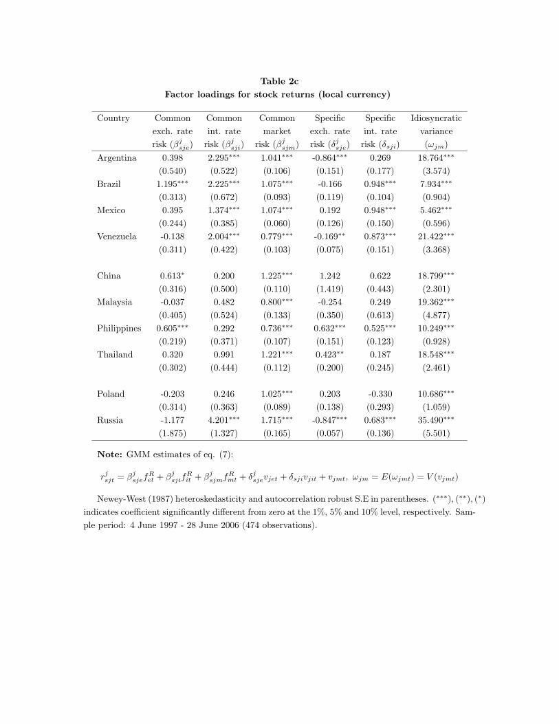
Table 2cFactor loadings for stock returns (local currency)

Country Common Common Common Speci�c Speci�c Idiosyncratic

exch. rate int. rate market exch. rate int. rate variance

risk (�jsje) risk (�jsji) risk (�jsjm) risk (�jsje) risk (�sji) (!jm)

Argentina 0.398 2.295�� 1.041�� -0.864�� 0.269 18.764��

(0.540) (0.522) (0.106) (0.151) (0.177) (3.574)

Brazil 1.195�� 2.225�� 1.075�� -0.166 0.948�� 7.934��

(0.313) (0.672) (0.093) (0.119) (0.104) (0.904)

Mexico 0.395 1.374�� 1.074�� 0.192 0.948�� 5.462��

(0.244) (0.385) (0.060) (0.126) (0.150) (0.596)

Venezuela -0.138 2.004�� 0.779�� -0.169�� 0.873�� 21.422��

(0.311) (0.422) (0.103) (0.075) (0.151) (3.368)

China 0.613� 0.200 1.225�� 1.242 0.622 18.799��

(0.316) (0.500) (0.110) (1.419) (0.443) (2.301)

Malaysia -0.037 0.482 0.800�� -0.254 0.249 19.362��

(0.405) (0.524) (0.133) (0.350) (0.613) (4.877)

Philippines 0.605�� 0.292 0.736�� 0.632�� 0.525�� 10.249��

(0.219) (0.371) (0.107) (0.151) (0.123) (0.928)

Thailand 0.320 0.991 1.221�� 0.423�� 0.187 18.548��

(0.302) (0.444) (0.112) (0.200) (0.245) (2.461)

Poland -0.203 0.246 1.025�� 0.203 -0.330 10.686��

(0.314) (0.363) (0.089) (0.138) (0.293) (1.059)

Russia -1.177 4.201�� 1.715�� -0.847�� 0.683�� 35.490��

(1.875) (1.327) (0.165) (0.057) (0.136) (5.501)

Note: GMM estimates of eq. (7):

rjsjt = �jsjef

Ret + �

jsjif

Rit + �

jsjmf

Rmt + �

jsjevjet + �sjivjit + vjmt; !jm = E(!jmt) = V (vjmt)




Table 3Wald Tests for pricing of idiosyncratic exchange rate and interest rates risks

Null

Hypothesis Risk Asset Fixed Floating

�cje = 0 8j Exchange rate Currencies 7.959 14.293

[0.159] [0.006]

�jbje = 0 8j Exchange rate Bonds 5.664 2.404

[0.340] [0.662]

�jsje = 0 8j Exchange rate Stocks 11.661 2.132

[0.040] [0.711]

�jbji = 0 8j Interest rate Bonds 9.855 5.377

[0.079] [0.251]

�jsji = 0 8j Interest rate Stocks 1.016 1.503

[0.961] [0.826]

Note: Newey-West (1987) heteroskedasticity and autocorrelation robust S.E. Sample period: 4June 1997 - 28 June 2006 (474 observations).

Table 4Net e¤ect of idiosyncratic exchange and interest rate volatility on returns

Asset Countries Average Wald p-value

Currencies ($) Fixed -0.015 0.202 0.653

Flexible 0.073 4.567 0.033

Di¤erence 0.087 3.737 0.053

Bonds (l.c.) Fixed -0.020 0.206 0.650

Flexible 0.055 3.807 0.051

Di¤erence 0.075 1.878 0.171

Stocks (l.c.) Fixed -0.002 0.001 0.982

Flexible -0.055 0.331 0.565

Di¤erence -0.053 0.223 0.637

Note: GMM estimates with Newey-West (1987) heteroskedasticity and autocorrelation robust

S.E. Sample period: 4 June 1997 - 28 June 2006 (474 observations).

Table 5Additional tests of market integration

Panel a: Test for pricing of idiosyncratic risksNull Latin Eastern

Hypothesis Risk Asset America Asia Europe

�cje = 0 8j Exchange rate Currencies 13.832 1.898 8.952

[0.008] [0.755] [0.011]

�jbje = 0 8j Exchange rate Bonds 2.421 5.299 26.102

[0.659] [0.258] [0.000]

�jsje = 0 8j Exchange rate Stocks 9.858 3.948 6.334

[0.043] [0.413] [0.042]

�jbji = 0 8j Interest rate Bonds 5.078 8.303 2.661

[0.279] [0.081] [0.264]

�jsji = 0 8j Interest rate Stocks 1.343 0.197 1.396

[0.854] [0.996] [0.498]

�jsjm = 0 8j Residual market Stocks 0.319 3.799 0.809

[0.989] [0.434] [0.667]

Panel b: Test for equality of common risk pricesNull Latin Eastern

Hypothesis Risk Asset America Asia Europe

�cje = 0 8j Exchange rate Currencies 7.119 58.636 9.162

[0.130] [0.000] [0.010]

�jbje = 0 8j Exchange rate Bonds 7.247 2.423 0.815

[0.123] [0.659] [0.665]

�jsje = 0 8j Exchange rate Stocks 3.569 5.224 0.982

[0.468] [0.265] [0.612]

�bji = 0 8j Interest rate Currencies 2.417 40.290 6.424

[0.660] [0.000] [0.040]

�jbji = 0 8j Interest rate Bonds 2.779 4.305 2.523

[0.596] [0.366] [0.283]

�jsji = 0 8j Interest rate Stocks 7.998 1.316 3.952

[0.092] [0.859] [0.139]

�cjm = 0 8j Residual market Currencies 6.595 60.833 5.154

[0.159] [0.000] [0.076]

�jbjm = 0 8j Residual market Bonds 3.503 2.362 0.867

[0.477] [0.670] [0.648]

�jsjm = 0 8j Residual market Stocks 8.384 3.474 0.391

[0.079] [0.482] [0.823]

Note: Newey-West (1987) heteroskedasticity and autocorrelation robust S.E. Sample period: 4June 1997 - 28 June 2006 (474 observations).

Table 6Average gains from stock market integration

Country �2sjm�m + !jm �sjm�m Di¤erence

Argentina 24.351�� 5.370�� 18.981��

(3.326) (0.761) (3.375)

Brazil 13.902�� 5.549�� 8.352��

(1.616) (0.694) (1.048)

Mexico 11.414�� 5.542�� 5.872��

(1.012) (0.580) (0.671)

Venezuela 24.551�� 4.018�� 20.533��

(3.615) (0.609) (3.404)

China 26.542�� 6.321�� 20.221��

(3.184) (0.833) (2.676)

Malaysia 22.668�� 4.130�� 18.538��

(5.854) (0.803) (5.142)

Philippines 13.041�� 3.796�� 9.246��

(1.339) (0.610) (0.969)

Thailand 26.236�� 6.298�� 19.937��

(3.229) (0.712) (2.858)

Poland 16.110�� 5.290�� 10.819��

(1.597) (0.705) (1.124)

Russia 50.671�� 8.851�� 41.820��

(7.360) (1.135) (6.570)

Note: GMM estimates with Newey-West (1987) heteroskedasticity and autocorrelation robust

S.E in parantheses. (��); (��); (�) indicates coe¢ cient signi�cantly di¤erent from zero at the 1%,

5% and 10% level, respectively. Sample period 4 June 1997 - 28 June 2006 (474 observations).

Figure 1(a) Average Conditional Standard Deviation of Idiosyncratic Exchange Rate Factors

0

1

2

3

4

5

6

7

Jun

97

Oct

97

Feb

98

Jun

98

Oct

98

Feb

99

Jun

99

Oct

99

Feb

00

Jun

00

Oct

00

Feb

01

Jun

01

Oct

01

Feb

02

Jun

02

Oct

02

Feb

03

Jun

03

Oct

03

Feb

04

Jun

04

Oct

04

Feb

05

Jun

05

Oct

05

Feb

06

Jun

06

Std.

Dev

.

Fixed Flex

(b) Average Conditional Standard Deviation of Idiosyncratic Interest Rate Factors

0

0.5

1

1.5

2

2.5

3

3.5

Jun

97

Oct

97

Feb

98

Jun

98

Oct

98

Feb

99

Jun

99

Oct

99

Feb

00

Jun

00

Oct

00

Feb

01

Jun

01

Oct

01

Feb

02

Jun

02

Oct

02

Feb

03

Jun

03

Oct

03

Feb

04

Jun

04

Oct

04

Feb

05

Jun

05

Oct

05

Feb

06

Jun

06

Std.

Dev

.

Fixed Flex

Figure 2(a) Net E¤ect of Idiosyncratic Exchange Rate Volatility on Currency Returns

0.7

0.6

0.5

0.4

0.3

0.2

0.1

0

0.1

0.2

0.3

Jun

97

Oct

97

Feb

98

Jun

98

Oct

98

Feb

99

Jun

99

Oct

99

Feb

00

Jun

00

Oct

00

Feb

01

Jun

01

Oct

01

Feb

02

Jun

02

Oct

02

Feb

03

Jun

03

Oct

03

Feb

04

Jun

04

Oct

04

Feb

05

Jun

05

Oct

05

Feb

06

Jun

06

Fixed Flex

(b) Net E¤ect of Idiosyncratic Exchange Rate and Interest Rate Volatility on Bond Returns

1

0.8

0.6

0.4

0.2

0

0.2

0.4

0.6

Jun

97

Oct

97

Feb

98

Jun

98

Oct

98

Feb

99

Jun

99

Oct

99

Feb

00

Jun

00

Oct

00

Feb

01

Jun

01

Oct

01

Feb

02

Jun

02

Oct

02

Feb

03

Jun

03

Oct

03

Feb

04

Jun

04

Oct

04

Feb

05

Jun

05

Oct

05

Feb

06

Jun

06

Fixed Flex

(c) Net E¤ect of Idiosyncratic Exchange Rate and Interest Rate Volatility on Stock Returns

2

1.5

1

0.5

0

0.5

1

Jun

97

Oct

97

Feb

98

Jun

98

Oct

98

Feb

99

Jun

99

Oct

99

Feb

00

Jun

00

Oct

00

Feb

01

Jun

01

Oct

01

Feb

02

Jun

02

Oct

02

Feb

03

Jun

03

Oct

03

Feb

04

Jun

04

Oct

04

Feb

05

Jun

05

Oct

05

Feb

06

Jun

06

Fixed Flex

exchange rate regimes, globalisation, and the cost of ... · exchange rate regimes, globalisation,...

Documents