exchange rate volatility and the performance of
TRANSCRIPT

Proceedings of the 2nd
International Conference, The Federal Polytechnic, Ilaro, 10th
– 11th
Nov., 2020
1955 Isiaka, Najeem Ayodeji & Olayiwola, Habeeb Olaniyi
EXCHANGE RATE VOLATILITY AND THE PERFORMANCE OF
MANUFACTRUING SECTOR IN NIGERIA: ARCH MODELING APPROACH.
Isiaka, Najeem Ayodeji & Olayiwola, Habeeb Olaniyi Department of Banking and Finance
Federal Polytechnic,Ilaro
Abstract
This study investigated the effect of exchange rate volatility on the performance of manufacturing sector in Nigeria
for the period of 30years (i.e 1988-2017). The time series and secondary source of data were used. The data on real
exchange rate, exchange rate volatility, inflation rate, money supply, capacity utilization, government expenditure,
electricity consumption, trade openness and manufacturing output share of GDP were gathered from Central Bank
of Nigeria (CBN) statistical bulletin. The ARCH and GARCH modeling techniques was employed to test for
volatility in exchange rate and its effect on the performance of manufacturing sector. Other tests include the
Augmented Dickey Fuller (ADF) test; correlation matrix test; Johansen cointegration test; and Vector Error
Correction Method (VECM) among others were considered in the study. The findings revealed that exchange rate
volatility has a positive and significant effect on the performance of manufacturing sector in Nigeria for the period
under review. The study concludes that exchange rate if properly managed serves as catalyst for the growth of
manufacturing sector in Nigeria. We therefore recommend among others that the policy maker should stabilize the
exchange rate for the benefit of manufacturing sectors by tightening the loopholes against black markets of foreign
currencies.
Keywords: Exchange Rate, Inflation rate, Manufacturing Sector, Volatility.
Introduction
In a modern economy, one of the factors that reflect the strength of a particular country is the ability to produce
sufficient and quality goods and services for domestic consumption and sales at the international market. Ojeyinka
(2019) as cited in Fakiyesi (2005) posits that increased manufacturing sector outputs can contribute immensely to
the growth process by providing import substitution, foreign exchange earnings, export expansion as well as creating
employment opportunities in the country. Thus, the manufacturing sector becomes an accelerator for the pace of
structural transformation and diversification of the economy, which reduces the level of foreign demands and
encourages local utilization of raw materials. Manufacturing sector is assumed to be more dynamic than other
sectors like agricultural sector due to its conversion of raw materials to finished goods that enhances a nation’s
output within a certain period. Consequently, the performance of manufacturing sector in Nigeria has been
questioned and subjected to constant reviews (Adediran & Obasan, 2010).
Though manufacturing sector has experienced a steady growth between 1990 and 2015, the sudden decline which
was attributed to several challenges had gone beyond the control of the sector. One of these problems is basically an
overreliance on the importation of raw materials and the removal of 41 items from the lists of users of foreign
exchange by the Nigerian government coupled with the drop in the naira to dollar exchange rate. The high cost of
sourcing dollar made it difficult for the firms to bring in their raw materials and those that were able to pay do not
even get the dollars supplied to them promptly. Therefore, the big to fall in the sector recorded huge drop in
patronage, turnover and profit margins as well as decline in production, layoffs, reduction and non-payment of
staff’s salaries and factory closure. These challenges added to the recessionary gap in the country as the production
Proceedings of the 2nd
International Conference, The Federal Polytechnic, Ilaro, 10th
– 11th
Nov., 2020
1956 Isiaka, Najeem Ayodeji & Olayiwola, Habeeb Olaniyi
was dropping drastically, spiking inflationary pressure, spiral in cyclical and structural unemployment were
skyrocketing and most especially, volatility in the exchange rate caused more havoc to the manufacturing sector.
Meanwhile many countries involve in exchanging of goods and services are directly or indirectly connected with
other economies of the world and hence exchange of foreign currencies become paramount (Adedokun, 2012).
However, the misalignment in exchange rate, unstable foreign exchange polices and large variation in exchange rate
movement can leads to contraction in manufacturing performance, productivity and result to economic hardship
(Umar & Soliu, 2009). Holding to the fact that exchange rate were influenced through different factors and
intensities. It becomes difficult for manufacturing sectors to predict movement of exchange rate except the market
dealers. Predicting this movement may likely leads to high volatility in the market. Ajao and Igbekoyi (2013)
viewed volatility as the rate which is associated with unpredictable movements in the relative price of foreign
currency in the market. Aliyu (2008) also explained volatility of exchange rate as a situation in which a country’s
actual exchange rate deviates from such an unobservable equilibrium. An exchange rate is said to be “undervalued”
when it depreciates more than its equilibrium, and “overvalued” when it appreciates more than its equilibrium.
Most importantly, depreciation of exchange rate raises the cost of imported capital goods, which would lead to a fall
in domestic investment and spike in inflationary pressure (Jongbo, 2014). However, some theoretical evidences
suggested that an alignment of exchange rate has a crucial influence on the growth rate of per capita output of an
open economies and low income countries (Opeluwah,Umeh &Ameh,2010). Despite the enormous researches
related to exchange rate volatility and performance of manufacturing sector, the topic still remains the major area of
interest to finance experts, researchers and economist so as to determine the major factors causing disequilibria in
exchange rate movement and its effect on manufacturing sector (Ajao & Igbekoyi,2013). Yet, there has no explicitly
specified answer to what determine the exchange rate volatility; this means that the concept of exchange rate
volatility remains subjective. Hence, exchange rate stability is one of the main factors influencing the productivity of
manufacturing sector in the country. Against this background, that the study controlled for openness to trade,
money supply, recurrent expenditure, capacity utilization, electricity consumption of manufacturing sector and
volatility of exchange rate as it affects the performance of manufacturing sector. This was carried out using ARCH
and GACH modeling to know if volatility in exchange rate influenced manufacturing performance during the period
of 30 years between 1988 and 2017.
Literature Reviews
The debates among the researchers regarding the influence of exchange rate volatility on manufacturing sector
remain unsettled. The exchange rate policies in developing countries are often sensitive and controversial mainly
because of the kind of structural transformation required. The policy such as reducing imports or expanding non-oil
exports invariably implies a depreciation of the exchange rate. Such domestic adjustments due to their short-run
impact on prices and demand are perceived as damaging to the economy. Exchange rate movement is essentially
significant in today’s economy because of the huge trading volume between countries. Anyawu, (2001) commented
as follows: “prolonged economic recession occasioned by the collapse of the world oil market from early 1980s and
the attendant sharp fall in foreign exchange earnings have adversely affected various source of economic growth and
development in Nigeria. In 2017, other problems of the economy include excessive dependence on imports for
consumption and capital goods, dysfunctional social and economic infrastructure, unprecedented fall in capital
utilization in industry and neglect of the agricultural sector amongst others.
Aluko, Akinola and Fatokun (2004) also reiterate that one of the greatest problems of the Nigerian economy is the
problem of capacity utilization in the manufacturing sector. This problem became more pronounced and aggravated
by the Structural Adjustment Programme (SAP) introduced in 1986 and recently, by globalization, and
internalization policy of financial transactions and all that accompanied them. In their study, the evaluation was
characterized by the following indices; low capacity utilization which averaged 30% in the last decade, low and
declining contribution to national output, which averaged 6%, declining and negative growth rates, low value added
to production due to high import dependence for inputs, accumulation of large inventories of unsold goods,
dominance of substandard goods, which cannot compete internationally. It was further attributed by the researchers
that the dependable conditions of the manufacturing sector to a horde of factors like lack of an enabling
environment, which include policy and political instability, poor macroeconomic environment, poor legal
environment which could not guarantee property right and safety, and lack of good governance. Others include poor

Proceedings of the 2nd
International Conference, The Federal Polytechnic, Ilaro, 10th
– 11th
Nov., 2020
1957 Isiaka, Najeem Ayodeji & Olayiwola, Habeeb Olaniyi
and inadequate infrastructure, poor implementation of incentives to manufacturing, including export incentives, low
access to investible funds due to underdeveloped long term capital budget.
The growth rate of manufacturing sector in a country depends on other variables beyond exchange rate, such as price
level stability which steps down stability. Specifically, the country’s level of infrastructural development such as;
electricity, good network of interlinked roads, ICT, effective communication and security of lives and property are
the major factors to enhance the productivity of manufacturing sectors in Nigeria. More so, sophisticated of health
system, stable health system and access to medicare by the workers equally improve the healthy state and improve
life expectancy of workers. Also, a stable tax policy, that eradicate major complaints of double taxation where
government introduced different tax regimes thereby increasing production cost. Subsequently, the development of
manpower particularly in the key sectors of the economy will reduce brain drain. The sector should be seen as one of
the potent tools for tackling developmental issues of state. Most of the developed countries are strong enough in
their manufacturing sector.
Theoretically, the study review and unpinned the base of the study to the popular Cobb-Douglas theory of
production. The theory is widely used to represent the relationship of an output to inputs. In economics, total-factor
productivity (TFP) is a variable which accounts for effects in total output not caused by inputs. For example, a year
with unusually good weather will tend to have higher output, because bad weather hinders agricultural output. A
variable like weather does not directly relate to unit inputs, so weather is considered a total-factor productivity
variable. (Wikipedia, 2015). The equation below (in Cobb-Douglas) represents total output (Y) as a function of
total-factor productivity (A), capital input (K), labor input (L), and the two inputs' respective shares of output (α is
the capital input share of contribution). An increase in either A, K and L will lead to an increase in output. While
capital and labor input are tangible, total-factor productivity appears to be more intangible as it can ranch from
technology to knowledge of worker (human capital). The reason why Cobb-Douglas equation is used in this function
is because it exhibits constant return to scale. That is, if we double input, we get a double output.
Technology Growth and Efficiency are regarded as two of the biggest sub-sections of Total Factor Productivity, the
former possessing "special" inherent features such as positive externalities and non- rival which enhance its position
as a driver of economic growth. Total Factor Productivity is often seen as the real driver of growth within an
economy and studies reveal that whilst labour and investments are important contributors, Total Factor Productivity
may account for up to 60% of growth within economies.
Empirically, some evidences have been gathered from different countries of the world on exchange rate volatility
and the performance of manufacturing sector. In India, Dhasamana (2013) wrote on the real effective exchange rate
and manufacturing sector performance, the paper noted that the there is a long run effect between exchange rate and
manufacturing sector in Indian. The empirical analysis of the paper shows that real exchange rate movement has a
significant impact on Indian firms’ performance through cost as well as revenue channel. In Canada, Frigon (2013)
researched on the exchange rate fluctuations and competiveness of the Canadian manufacturing sector and selected
industrialised nations. It was discovered that the gains of the Canadian dollar against the US dollar over the past
decade has led to the decline in the competitiveness of the Canadian manufacturing sector. Between the year 2000
and 2011 the economic structure of Canada has undergone a major makeover which allows the manufacturing
sector’s GDP to fall by 1.4% yearly, while from 1997 to 2011 the GDP of the manufacturing sector grew by 0.5%
till it started to fall from the new millennium. It was also noted that due to foreign exchange fluctuations only
Canada manufacturing industry shrank compared to other developed countries. The comparative analysis showed in
his paper shows that the gaining of Canadian dollar against the US dollar has led to decline of GDP from the
manufacturing sector.
In United State, Olivie (2002) assessed exchange rates and the prices of manufacturing products imported into the
United States. It was submitted in the study that exchange rate fluctuations remain remarkably large, despite the
steady decline in the volatility of the trade-weighted dollar since the late 1980s. Yet, large fluctuations in the value
of the dollar do not translate into similarly large swings in the domestic production of traded goods relative to
foreign currency. This article re-examines the responsiveness of U.S. import prices to changes in the exchange rate
in a sample of manufacturing industries over the past two decades. It documents a decline in the estimated pass

Proceedings of the 2nd
International Conference, The Federal Polytechnic, Ilaro, 10th
– 11th
Nov., 2020
1958 Isiaka, Najeem Ayodeji & Olayiwola, Habeeb Olaniyi
through elasticity for most industries in the 1990s. For the industries in their sample, pass-through was 0.50 on
average in the 1980s and dropped to an average of about 0.25 in the 1990s. This finding suggests that larger changes
in the exchange rate are now needed to move the dollar price of imported goods relative to the price of domestic
goods.
Evidences from Nigeria, Nwokoro (2017) investigated the impact of foreign exchange and interest rates variations
on the Nigeria’s manufacturing Output during the period 1983 to 2014. It was revealed that Foreign Exchange Rate
(FREX) and Interest Rates (INTR) have negative but significant relationship with manufacturing Output (MANO).
In the same vein, Oyati (2016) in her research paper titled: “Relevance, prospects and challenges of manufacturing
sector in Nigeria asserted the fact that manufacturing is the hub of a vibrant and stable national economy. It also
stated that for the sector to remain relevant, various available raw materials should be harnessed, processed and
transformed to either finished goods or semi-finished goods. The challenges the researcher noticed in the sector was
poor availability of power, poor infrastructures, irregular taxes, poor business development strategies e.t.c. The
paper articulates various strategies that stakeholders in the manufacturing sector can consider in order to re-position
the industry for national economic growth for robust performance with consequent national economic growth. The
research work by Lawal (2016) examined the effect of exchange rate fluctuations on manufacturing sector output in
Nigeria from 1986 to 2014, a period of 28 years. Data sourced from Central Bank of Nigeria (CBN) statistical
Bulletin and World Development Indicators (WDI) on manufacturing output, Consumer Price Index (CPI),
Government Capital Expenditure (GCE) and Real Effective Exchange Rate (EXC) were analyzed through the
multiple regression analysis using Autoregressive Distribution Lag (ARDL) to examine the effect of exchange rate
fluctuations on manufacturing sector. Using ARDL it was discovered that exchange rate fluctuations have long run
and short run relationship on manufacturing sector output. The result showed that exchange rate has a positive
relationship on manufacturing sector output but not significant. However, from the empirical analysis it was
discovered that exchange rate is positively related to manufacturing sector output.
Ajao and Igbekoyi (2013), in their research paper, investigate the determinants of real exchange rate volatility in
Nigeria from 1981 through 2008. They obtained volatility of exchange rate through the GARCH (1,1) techniques.
Empirical analysis further shows that openness of the economy, government expenditures, interest rate movements
as well as the lagged exchange rate are among the major significant variables that influence REXRVOL during this
period. Akpan and Atan (2013) researched on the effects of exchange rates movement on real output growth in
Nigeria. The research was used in determining direct and indirect relationship between exchange rates and GDP
growth. Generalized Method of Moments (GMM) was employed to determine the relationship which was derived
using a simultaneous equation model within a macroeconomic model for the year 1986-2010. The result shows an
evidence of strong growth between changes in exchange rate and output growth. The conclusion of the research is
that improvements in exchange rates are necessary but not enough to revive the Nigerian economy.
Methodology
This study contributed to the existing knowledge by investigated the effect of exchange rate volatility on the
performance of manufacturing sector in Nigeria between 1988 and 2017 covering the period of tight exchange rate
regime and recessionary gap in the economy. The data employed in this study were obtained from the publications
of the Central Bank of Nigeria (CBN) Statistical Bulletin; Data were also sorted from the National Bureau of
Statistics. Generally, the data used for the study are known as secondary data, which are time series data recorded
over the years. The variables considered in the study are real exchange rate, exchange rate volatility, inflation rate,
money supply , capacity utilization, government expenditure, electricity consumption, trade openness and
manufacturing output for the period of 30 years spanning from 1988-2017. In testing for the presence of volatility in
the series, this study shall the autoregressive conditional heteroscedasticity (ARCH) and the Generalised
Autoregressive Conditional Heteroscedasticity (GARCH) model. In order to model the impact of exchange rates and
their volatility on manufacturing output, and a multiple linear regression model has been constructed.
Measurement of volatility
Econometric technique will be used to analyze the effect of exchange rate volatility on the performance of
manufacturing sector in Nigeria. The ARCH and GARCH (1, 1) family model is used to measure exchange rate
volatility and the conditional variance series generates the volatility data from 1988 – 2017. It is believed that the
Proceedings of the 2nd
International Conference, The Federal Polytechnic, Ilaro, 10th
– 11th
Nov., 2020
1959 Isiaka, Najeem Ayodeji & Olayiwola, Habeeb Olaniyi
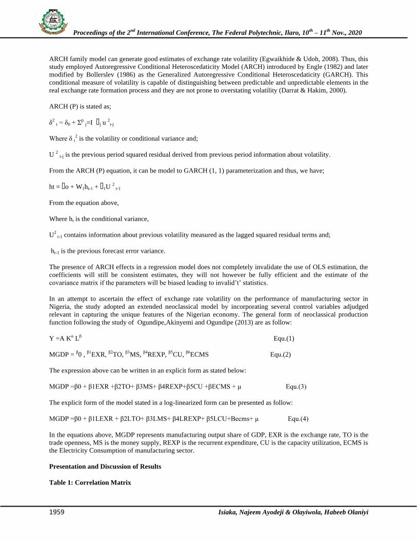
ARCH family model can generate good estimates of exchange rate volatility (Egwaikhide & Udoh, 2008). Thus, this
study employed Autoregressive Conditional Heteroscedaticity Model (ARCH) introduced by Engle (1982) and later
modified by Bollerslev (1986) as the Generalized Autoregressive Conditional Heteroscedaticity (GARCH). This
conditional measure of volatility is capable of distinguishing between predictable and unpredictable elements in the
real exchange rate formation process and they are not prone to overstating volatility (Darrat & Hakim, 2000).
ARCH (P) is stated as;
δ2 t = δ0 + Σ
p j=I ϒj u
2t-j
Where δ t2 is the volatility or conditional variance and;
U 2 t-j is the previous period squared residual derived from previous period information about volatility.
From the ARCH (P) equation, it can be model to GARCH (1, 1) parameterization and thus, we have;
ht = ϒo + W1ht-1 + ϒ1U 2 t-1
From the equation above,
Where ht is the conditional variance,
U2 t-1 contains information about previous volatility measured as the lagged squared residual terms and;
ht-1 is the previous forecast error variance.
The presence of ARCH effects in a regression model does not completely invalidate the use of OLS estimation, the
coefficients will still be consistent estimates, they will not however be fully efficient and the estimate of the
covariance matrix if the parameters will be biased leading to invalid’t’ statistics.
In an attempt to ascertain the effect of exchange rate volatility on the performance of manufacturing sector in
Nigeria, the study adopted an extended neoclassical model by incorporating several control variables adjudged
relevant in capturing the unique features of the Nigerian economy. The general form of neoclassical production
function following the study of Ogundipe,Akinyemi and Ogundipe (2013) are as follow:
Y =A Kα L
β Equ.(1)
MGDP = β0 ,
β1EXR,
β2TO,
β3MS,
β4REXP,
β5CU,
β6ECMS Equ.(2)
The expression above can be written in an explicit form as stated below:
MGDP =β0 + β1EXR +β2TO+ β3MS+ β4REXP+β5CU +βECMS + µ Equ.(3)
The explicit form of the model stated in a log-linearized form can be presented as follow:
MGDP =β0 + β1LEXR + β2LTO+ β3LMS+ β4LREXP+ β5LCU+Βecms+ µ Equ.(4)
In the equations above, MGDP represents manufacturing output share of GDP, EXR is the exchange rate, TO is the
trade openness, MS is the money supply, REXP is the recurrent expenditure, CU is the capacity utilization, ECMS is
the Electricity Consumption of manufacturing sector.
Presentation and Discussion of Results
Table 1: Correlation Matrix

Proceedings of the 2nd
International Conference, The Federal Polytechnic, Ilaro, 10th
– 11th
Nov., 2020
1960 Isiaka, Najeem Ayodeji & Olayiwola, Habeeb Olaniyi
LMGDP LEXR LTO MS REXP LCAUT LMSEC
LMGDP 1.000000 0.933944 -0.426144 0.823584 0.882912 0.631538 0.763794
LEXR
1.000000 -0.254185 0.667695 0.764499 0.668710 0.652268
LTO
1.000000 -0.756411 -0.671670 -0.315084 -0.628618
MS
1.000000 0.975742 0.618059 0.851948
REXP
1.000000 0.712792 0.897800
LCAUT
1.000000 0.777252
LMSEC 1.000000
Source: Authors’ Compilation from Eview 9
It is recognized that the issue of strong correlation between the explanatory variables may violate the working
assumptions of the estimation technique. We, therefore, examine the possibility of the presence of multi-collinearity
among the predictors in the model by examining the pair-wise correlation matrix as contained in Table 1. The table
indicates that there exists a significant positive correlation between LMGDP and LEXR; LMS; LREXP; LCAUT;
LMSEC except LTO that shows a negative correlation with LMGDP. Overall, it can be established from the
magnitude of the correlation coefficients that multi-collinearity is not a potential problem in the models. Thus, the
data set in conjunction with the variables are appropriate for the study
Table 2: Unit Root
Augmented Dickey – Fuller (ADF)
Variables At Level OI Remarks First difference OI Remarks
LMGDP -0.848942 1(0) Non-stationary -6.950744* 1(1) Stationary
LEXR -1.949713 1(0) Non-stationary -5.157513* 1(1) Stationary
LTO -1.139313
1(0) Non-stationary -7.548999*
1(1) Stationary
LMS -2.559498 1(0) Non-stationary -2.917406***
1(1) Stationary (10%)
LREXP -2.282117
1(0) Non-stationary -7.380027*
1(1) Stationary
LCAUT -1.005410 I(0) Non-stationary -4.869716* 1(1) Stationary
LMSEC -0.545492
1(0) Non-stationary -6.341352*
1(1) Stationary
Source: Authors’ Compilation from Eview 9
Proceedings of the 2nd
International Conference, The Federal Polytechnic, Ilaro, 10th
– 11th
Nov., 2020
1961 Isiaka, Najeem Ayodeji & Olayiwola, Habeeb Olaniyi
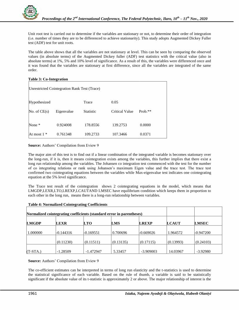
Unit root test is carried out to determine if the variables are stationary or not, to determine their order of integration
(i.e. number of times they are to be differenced to achieve stationarity). This study adopts Augmented Dickey Fuller
test (ADF) test for unit roots.
The table above shows that all the variables are not stationary at level. This can be seen by comparing the observed
values (in absolute terms) of the Augmented Dickey fuller (ADF) test statistics with the critical value (also in
absolute terms) at 1%, 5% and 10% level of significance. As a result of this, the variables were differenced once and
it was found that the variables are stationary at first difference, since all the variables are integrated of the same
order.
Table 3: Co-Integration
Unrestricted Cointegration Rank Test (Trace)
Hypothesized Trace 0.05
No. of CE(s) Eigenvalue Statistic Critical Value Prob.**
None * 0.924008 178.8556 139.2753 0.0000
At most 1 * 0.761348 109.2733 107.3466 0.0371
\ Source: Authors’ Compilation from Eview 9
The major aim of this test is to find out if a linear combination of the integrated variable is becomes stationary over
the long-run, if it is, then it means cointegration exists among the variables, this further implies that there exist a
long run relationship among the variables. The Johansen co integration test commenced with the test for the number
of co integrating relations or rank using Johansen’s maximum Eigen value and the trace test. The trace test
confirmed two cointegrating equations between the variables while Max-eigenvalue test indicates one cointegrating
equation at the 5% level significance.
The Trace test result of the cointegration shows 2 cointegrating equations in the model, which means that
LMGDP,LEXR,LTO,LREXP,LCAUTAND LMSEC have equilibrium condition which keeps them in proportion to
each other in the long run, means there is a long-run relationship between variables.
Table 4: Normalized Cointegrating Coefficients
Normalized cointegrating coefficients (standard error in parentheses)
LMGDP LEXR LTO LMS LREXP LCAUT LMSEC
1.000000 -0.144316 -0.169551 0.700696 -0.669026 1.964572 -0.947200
(0.11230) (0.11511) (0.13135) (0.17115) (0.13993) (0.24103)
(T-STA.) -1.28509 -1.472947 5.33457 -3.909003 14.03967 -3.92980
Source: Authors’ Compilation from Eview 9
The co-efficient estimates can be interpreted in terms of long run elasticity and the t-statistics is used to determine
the statistical significance of each variable. Based on the rule of thumb, a variable is said to be statistically
significant if the absolute value of its t-statistic is approximately 2 or above. The major relationship of interest is the

Proceedings of the 2nd
International Conference, The Federal Polytechnic, Ilaro, 10th
– 11th
Nov., 2020
1962 Isiaka, Najeem Ayodeji & Olayiwola, Habeeb Olaniyi
one that exists between exchange rate volatility and manufacturing output in Nigeria. From the table above exchange
rate is elastic in relation to manufacturing output, meaning that in the long run, a change in exchange rate volatility
will cause a more proportionate change of 14 percent in manufacturing output and the t-statistic of LEXR shows that
the co-efficient is statistically significant.
Table 5: Error Correction Method
Error
Correction: D(LMGDP) D(LEXR) D(LTO) D(LMS) D(LREXP) D(LCAUT) D(LMSEC)
CointEq1 -0.217314 0.019252 -0.248747 -0.084511 0.513508 0.007774 0.082059
(0.16326) (0.24496) (0.15754) (0.07597) (0.16702) (0.08047) (0.08599)
[-1.33111] [ 0.07859] [-1.57892] [-1.11242] [ 3.07457] [ 0.09660] [ 0.95424]
Source: Authors’ Compilation from Eview 9
The speed of adjustment co-efficient for LMGDP is -0.217314. The VECM is correctly signed and in terms of
magnitude it lies between 0 and 1. This significance supports cointegration as it shows that there exists a long run
steady equilibrium between manufacturing output and the explanatory variables. Precisely the error correction
model in this equation means that about 21.73 % of errors generated between each period are correlated in
subsequent periods. However, the result is insignificant judging from the value of the T-statistic [-1.33111].
Table 6: ARCH and GARCH Model
This section aims to test for the presence of volatility by employing the ARCH and GARCH model. Having
estimated the OLS regression of the model, the residual plot result for ascertaining the presence/absence of ARCH
and GARCH effect is presented in the figure below
-0.4
0.0
0.4
0.8
1.2
1.6
1
2
3
4
5
6
90 92 94 96 98 00 02 04 06 08 10 12 14 16
Residual Actual Fitted

Proceedings of the 2nd
International Conference, The Federal Polytechnic, Ilaro, 10th
– 11th
Nov., 2020
1963 Isiaka, Najeem Ayodeji & Olayiwola, Habeeb Olaniyi
The fluctuation is the residual, it is evident from the graph that there is a high volatility for short period of 1988 to
1999 and there is a low volatility between 2000 and 2010. This implies that period of high volatility are followed by
periods of high volatility for a short period while period of low volatility are followed by period of low volatility for
a long period. This suggested that the residual or error term is heteroscedastic and it can be represented by ARCH
and GARCH model.
Table 7 : Test of Serial Correlation of the GARCH (1.1)
Model: Correlogram Squared Residual
Date: 11/18/18 Time: 18:45
Sample: 1988 2017
Included observations: 30
Autocorrelation Partial Correlation AC PAC Q-Stat Prob*
. |***** | . |***** | 1 0.699 0.699 16.154 0.000
. |*** | . | . | 2 0.462 -0.051 23.466 0.000
. |**. | . *| . | 3 0.244 -0.116 25.587 0.000
. |* . | . |* . | 4 0.208 0.190 27.189 0.000
. |**. | . |**. | 5 0.290 0.231 30.429 0.000
. |**. | . *| . | 6 0.266 -0.136 33.262 0.000
. |* . | .**| . | 7 0.097 -0.281 33.653 0.000
. | . | . |* . | 8 -0.011 0.110 33.658 0.000
. *| . | . *| . | 9 -0.140 -0.126 34.551 0.000
. | . | . |**. | 10 0.012 0.280 34.558 0.000
. | . | . *| . | 11 0.050 -0.153 34.686 0.000
. | . | . | . | 12 0.064 -0.000 34.907 0.000
. | . | . | . | 13 -0.030 -0.058 34.957 0.001
. *| . | . | . | 14 -0.128 -0.002 35.938 0.001
. *| . | . *| . | 15 -0.187 -0.166 38.169 0.001
. *| . | . *| . | 16 -0.188 -0.157 40.602 0.001
*Probabilities may not be valid for this equation specification.

Proceedings of the 2nd
International Conference, The Federal Polytechnic, Ilaro, 10th
– 11th
Nov., 2020
1964 Isiaka, Najeem Ayodeji & Olayiwola, Habeeb Olaniyi
Autocorrelation Hypothesis
H0: There is no serial correlation.
H1: There is serial correlation.
The decision rule states that, if the p-values are more than 5%, we accept the null hypothesis (H0) and vice versa.
However, it is evident from the above result that virtually all the probability values chosen for the 17 different lags
are less than 5%, hence, we reject the null hypothesis (H0) and we accept the alternative hypothesis (H1). We can
therefore conclude that the estimated GARCH (1.0) model has serial correlation.
Table 8: Test of Normal Distribution: Jarque-Bera Statistics
Standard Dev. 1.002050
Skewness 0.404107
Kurtosis 1.898374
Jarque-Bera 2.333488
Probability 0.311379
Author’s Computation
The “Histogram Normality Test” will be employed to examining if the residuals of the estimated GARCH (1.0)
model are normally distributed using the Jarque-Bera statistics. Normal Distribution Hypothesis
H0: Residuals are normally distributed.
H1: Residuals are not normally distributed.
It is evident that the desirable from the above hypothesis is the null hypothesis; however, the result of the Jarque-
Bera statistics is presented below.
It is clear that the Jarque–Bera statistics estimated has probability value of 0.311378 to be more than 5%. This
implies that we accept the null hypothesis (H0) and reject the alternative hypothesis (H1); we therefore conclude that
the residuals in the GARCH (1.0) model are normally distributed.
Table 9:Heteroskedasticity Test: ARCH
F-statistic 23.17894 Prob. F(1,27) 0.0001
Obs*R-squared 13.39584 Prob. Chi-Square(1) 0.0003
There is arch test

Proceedings of the 2nd
International Conference, The Federal Polytechnic, Ilaro, 10th
– 11th
Nov., 2020
1965 Isiaka, Najeem Ayodeji & Olayiwola, Habeeb Olaniyi
Test of ARCH Effect the “ARCH LM Test” is used to check if the model has an ARCH effect. This is also known as
the test of heteroscedasticity. The result is discussed as follows. However, the desirable in the below hypothesis is
the null hypothesis.
ARCH Effect Hypothesis H0: There is no ARCH Effect
H1: There is ARCH Effect
The decision rule states that, if the p-value of the Observed R*squared is more than 5%, we accept the null
hypothesis (H0), and vice versa. Hence, since the probability value 0.003 of the observed R*squared is less than
0.05 level of significance. We therefore accept the alternative hypothesis (H1) and reject the alternative hypothesis
and concluded that the model has ARCH effect. Overall, it is evident from all the evaluations analyzed above that
the residuals of the estimated GARCH (1.1) model has serial correlation, normally distributed and no ARCH effect.
However, the estimators of this model are still consistent though there is a serial correlation, hence; the model is
useful for forecasting the behaviour of the Nigeria’s exchange rate and its determinants in real terms.
Table 10: Arch Model
Method: ML ARCH - Normal distribution (BFGS / Marquardt steps)
Sample: 1988 2017
Included observations: 30
Convergence achieved after 21 iterations
Coefficient covariance computed using outer product of gradients
Presample variance: backcast (parameter = 0.7)
GARCH = C(3) + C(4)*RESID(-1)^2
Variable Coefficient Std. Error z-Statistic Prob.
C 1.353705 0.213273 6.347274 0
LEXR 1.359882 0.060176 22.59854 0
Variance Equation
C 0.034055 0.054932 0.619952 0.5353
RESID(-1)^2 1.011117 0.906696 1.115167 0.2648
R-squared 0.871034 Mean dependent var 6.991791
Adjusted R-squared 0.866428 S.D. dependent var 1.60869
Durbin-Watson stat 0.593616 AKaike Criterio
1.623443
Schwarz Criterio 1.810269
Source: Eview 9
For the mean equation, the probability is significant and for the variance equation The Akaike criterion is 1.623443
and the Schwarz criterion is 1.810269. The mean equation as observed in table shown to be statistically significant

Proceedings of the 2nd
International Conference, The Federal Polytechnic, Ilaro, 10th
– 11th
Nov., 2020
1966 Isiaka, Najeem Ayodeji & Olayiwola, Habeeb Olaniyi
at 0.05. This statistical significance is observed in the variance equation. The ARCH effect is shown to be
statistically significant at 0.05. From the above results, we can proceed to model the volatility of exchange rate using
the GARCH.
Table 11: GARCH (1, 1) model
Dependent Variable: LMGDP
Method: ML ARCH - Normal distribution (BFGS / Marquardt steps)
Date: 01/02/19 Time: 14:13
Sample: 1988 2017
Included observations: 30
Convergence achieved after 25 iterations
Coefficient covariance computed using outer product of gradients
Presample variance: backcast (parameter = 0.7)
GARCH = C(3) + C(4)*RESID(-1)^2 + C(5)*GARCH(-1)
Variable Coefficient Std. Error z-Statistic Prob.
C 1.384315 0.239180 5.787749 0.0000
LEXR 1.355290 0.066233 20.46237 0.0000
Variance Equation
C 0.024379 0.063023 0.386830 0.6989
RESID(-1)^2 0.939756 0.915247 1.026778 0.3045
GARCH(-1) 0.092796 0.337333 0.275088 0.7832
R-squared 0.871781 Mean dependent var 6.991791
Adjusted R-squared 0.867202 S.D. dependent var 1.608690
S.E. of regression 0.586230 Akaike info criterion 1.678799
Sum squared resid 9.622621 Schwarz criterion 1.912332
Log likelihood -20.18199 Hannan-Quinn criter. 1.753508
Durbin-Watson stat 0.594109

Proceedings of the 2nd
International Conference, The Federal Polytechnic, Ilaro, 10th
– 11th
Nov., 2020
1967 Isiaka, Najeem Ayodeji & Olayiwola, Habeeb Olaniyi
Source: Eview 9
For the mean equation, the probability is significant and for the variance equation The Akaike criterion is 1.678799
and the Schwarz criterion is 1.912332. The result for the GARCH (1,1) is presented in table 3. While the intercept of
the mean equation is found to be statistically significant, that of the variance equation is found otherwise. Similarly,
while the coefficient of the ARCH effect is found to be statistically significant at 0.05, the GARCH effect is found
to be statistically insignificant. These findings indicate that the information about exchange rate volatility in the
previous periods do not significantly determine the current volatility in the variable. This suggests that the ARCH
effect dominates. However, since the sum of the two effects is, a value which is close to but overall, still above
unity, a shock at time will persist for many periods in the future which generally suggest a long memory.
Discussion and summary of findings
This study examines the effect of exchange rate volatility on the performance of manufacturing sector in Nigeria
empirically from 1988 to 2017. Exchange rate has poorly been managed over time and the time is long overdue to
salvage the situation from getting worse. The theoretical issue on exchange rate was discussed and empirical finding
were done to know the past findings on exchange rate volatility. The Augmented Dickey Fuller (ADF) test was
carried out to test for unit roots for the variables involved. Correlation matrix was tested to check for the presence of
multi-collinearity or not among the variables. Johansen cointegration test was used to determine whether there is
long-run relationship among the variables and the results reveal the presence of two co-integration equations which
indicate the existence of long run relationship among variables. The vector error correction method (VECM) was
used to known whether there is any effect in the long run, a change in exchange rate volatility will cause a more
proportionate change of 14 percent in manufacturing output and the t-statistic of LEXR shows that the co-efficient
is statistically significant.
Conclusion and Recommendations
The findings show that exchange rate volatility has a positive and significant effect on the performance of
manufacturing sector in Nigeria for the period under review. The study therefore concludes that exchange rate if properly managed serves as catalyst for the growth of manufacturing sector in Nigeria. Based on the findings and
conclusions, the study recommends that during recession period, it is better and effective to relax monetary policies
and use expansionary polices to return the economy back to normal.
References
Ajao, M. G. & Igbekoyi, O. E. (2013). The determinants of real exchange rate volatility in Nigeria. Academic Journal of Interdisciplinary Studies, 2(1), 459-471
Akpan, E.O & Atan, J.A (2010). Effects of exchange rate movements on economic growth in Nigeria. CBN Journal
of Applied Statistics,4(2),23-45
Aliyu,S.U.R., (2008).Exchange rate volatility and export trade in Nigeria.An empirical investigation. Munich
Policians Economics. 3(5)34-46.
Arize, A. (1995), The effects of exchange rate volatility on U.S. exports: an empirical investigation. Southern
Economic Journal, 6(2), 34-43
Bollerslev, T. (1986) Generalised antrogressive conditional heteroscedasticity. Journal of Econometric. 3(1), 307-
327
Engle, R.F. (1982) Autoregressive conditional heteroscedasticity with estimates of the variance of United Kingdom Inflation, Econometrica. 5(10),987-1008

Proceedings of the 2nd
International Conference, The Federal Polytechnic, Ilaro, 10th
– 11th
Nov., 2020
1968 Isiaka, Najeem Ayodeji & Olayiwola, Habeeb Olaniyi
Fakiyesi, O. A. (2005). Issues money, finance and economic management Lagos: University press.
Jongbo, O. C. (2014). The impact of real exchange rate fluctuation on industrial output In Nigeria. Journal of Policy
and Development Studies.9, (1).268-279
Lawal, E. O.,(2016). Effect of exchange rate fluctuations on manufacturing sector output in Nigeria. Journal of
Research in Business and Management. 4( 10), 32-39
Nwokoro, A. N.,(2017). Foreign exchange and interest rates and manufacturing output in Nigeria. International
Journal of Business & Law Research 5(1):30-38
Obadan, M.I. (2006). Overview of exchange rate management in Nigeria 1986 to date, in the dynamics of exchange rate to Nigeria. Central Bank of Nigeria, Bulletin,30(3),10-30
Ogundipe A.A, Akinyemi, P, & Ogundipe O.M, (2013). Estimating the Long-run Effect of Exchange Rate Devaluation on the trade balance in Nigeria. European Scientific Journal. 9(25),15-45
Ojeyinka, T. A. (2019). Exchange rate volatility and the performance of manufacturing sector in Nigeria. African
Journal of Economic Review, 7(2), 27-41
Olivie P. Giovanni (2002).Exchange rates and the prices of Manufacturing Product. 2998imported into the United
States”, First Quarter 2002, New England Economic Review.
Oyati (2016). The Relevance, Prospects and the Challenges of the Manufacturing Sector
in Nigeria, (accessible at http://globalacademicgroup.com/journals/the%20intuition/The%20Relevance,%20P
rospects%20and%20the%20Challenges%20of%20the%20Manufactu.pdf Last accessed 03-03-2018.