MŰHELYTANULMÁNYOK DISCUSSION PAPERS

INSTITUTE OF ECONOMICS, CENTRE FOR ECONOMIC AND REGIONAL STUDIES,

HUNGARIAN ACADEMY OF SCIENCES - BUDAPEST, 2018

MT-DP – 2018/33

Exchange rates and prices:

a continuous wavelet perspective

GÁBOR ULIHA – JÁNOS VINCZE

Discussion papers

MT-DP – 2018/33

Institute of Economics, Centre for Economic and Regional Studies,

Hungarian Academy of Sciences

KTI/IE Discussion Papers are circulated to promote discussion and provoque comments.

Any references to discussion papers should clearly state that the paper is preliminary.

Materials published in this series may subject to further publication.

Exchange rates and prices: a continuous wavelet perspective

Authors:

Gábor Uliha OTP Bank Nyrt.

email: gabor.uliha@gmail.com

János Vincze research advisor

Center for Economic and Regional Studies, Hungarian Academy of Sciences and Corvinus University of Budapest email: janos.vincze@uni-corvinus.hu

December 2018

Exchange rates and prices:

a continuous wavelet perspective

Gábor Uliha – János Vincze

Abstract

In this paper we analyze statistics derived from the cross-wavelet transform of inflation

differentials and exchange rate changes for a group of countries with Germany as the

reference country. An important tool is the wavelet coherency measure from which we can

judge the strength of the price-exchange rate nexus at different time scales, and also whether

it has changed in time. Complex cross-wavelets provide information about phase

relationship, and we can investigate whether there is any consistent pattern in the lead-lag

relationship between prices and exchange rates. Also, we calculate a summary measure,

based on singular value decomposition, that shows which countries have significantly similar

inflation differential – exchange rate change processes. Our results accord, in some ways,

with former findings, but suggest an even gloomier view on the possibility of finding

statistically reliable relationships between exchange rates and aggregate price indices (CPI or

PPI). In line with the literature we haven’t found strong co-movement between prices and

exchange rates in the short or medium term. There are only weak indications that at least in

some countries the price-exchange rate connection strengthened during the crisis, and

detectable cycles at business cycle frequencies do not appear at all. Though by and large the

lead-lag relationship between prices and exchange rates is the expected one, still this is

unstable practically for every country. Results with respect to the PPI are more promising.

The three countries that seem to be closest to theoretical expectations are Sweden, Japan and

South-Korea. It is possible that the coherence between exchange rates and prices on the

macro level may depend more on similarities of export structure than on trading relations,

that microeconomic intuition would suggest. Also it is possible that macro price indices are

too noisy by their very nature to be amenable for statistical analyses not committed to strong

presumptions.

Keywords: real exchange rates, exchange rate pass-through, continuous wavelet analysis

JEL-codes: E31, C14, F41

Árfolyamok és árak: egy folytonos wavelet elemzés

Uliha Gábor – Vincze János

Összefoglaló

Ebben a tanulmányban a nominális árfolyamok és az inflációs különbségek összefüggését

elemezzük 19 országra a folytonos wavelet transzformáció segítségével. Referencia országnak

Németországot választottuk. Legfőbb analitikus eszközünk a wavelet koherencia, amely képes

a kapcsolatok erősségét időtávokra és időpontokra is értelmezni, továbbá számot adni arról,

hogy melyik idősor vezet és melyik követ. Különböző összegző mértékeket is kiszámítottunk,

amelyekből a kapcsolatok általános erősségére tehetünk megállapításokat. Eredményeink sok

tekintetben hasonlóak a más módszerekkel elért kvalitatív megállapításokhoz, de bizonyos

értelemben sötétebb képet festenek, amennyiben kevés konzisztens minta létszik

kirajzolódni, még olyan esetekben is, amelyekben ilyet a priori elvárnánk. (Ilyen például

Dánia esete.) Sem rövid, sem középtávon nem találunk általában szoros kapcsolatot, és nem

tűnik úgy, hogy a válság felerősítette volna az együttmozgást. Bár a vezető-követő kapcsolat

nagyjából megfelel a várakozásoknak, túlságos instabil ahhoz, hogy megbízható előrejelzések

alapjául szolgálhatna. A CPI-hez képest a PPI-vel elért eredmények inkább bíztatók, ismét

összhangban az eddigi irodalommal. Svédország, Japán és Dél-Korea az a három ország,

amely leginkább az elméleti várakozásoknak megfelelően viselkedik. Ez arra utalhat, hogy

nem annyira a kereskedelem intenzitása, mint inkább strukturális hasonlóságok játszhatnak

szerepet az aggregált árindexek és az árfolyamok együttmozgásában.

Tárgyszavak: reálárfolyam, árfolyam-ár kapcsolat, folytonos wavelet elemzés

JEL kódok: E31, C14, F41

Exchange rates and prices: a continuous wavelet perspective

Gábor Uliha

OTP Bank

(gabor.uliha@gmail.com)

János Vincze

Corvinus University of Budapest and Center for Economic and Regional Studies (Hungarian Academy of Sciences)

(janos.vincze@uni-corvinus.hu)

Abstract In this paper we analyze statistics derived from the cross-wavelet transform of inflation

differentials and exchange rate changes for a group of countries with Germany as the reference

country. An important tool is the wavelet coherency measure from which we can judge the

strength of the price-exchange rate nexus at different time scales, and also whether it has

changed in time. Complex cross-wavelets provide information about phase relationship, and we

can investigate whether there is any consistent pattern in the lead-lag relationship between

prices and exchange rates. Also, we calculate a summary measure, based on singular value

decomposition, that shows which countries have significantly similar inflation differential –

exchange rate change processes. Our results accord, in some ways, with former findings, but

suggest an even gloomier view on the possibility of finding statistically reliable relationships

between exchange rates and aggregate price indices (CPI or PPI). In line with the literature we

haven’t found strong co-movement between prices and exchange rates in the short or medium

term. There are only weak indications that at least in some countries the price-exchange rate

connection strengthened during the crisis, and detectable cycles at business cycle frequencies

do not appear at all. Though by and large the lead-lag relationship between prices and exchange

rates is the expected one, still this is unstable practically for every country. Results with respect

to the PPI are more promising. The three countries that seem to be closest to theoretical

expectations are Sweden, Japan and South-Korea. It is possible that the coherence between

exchange rates and prices on the macro level may depend more on similarities of export

structure than on trading relations, that microeconomic intuition would suggest. Also it is

possible that macro price indices are too noisy by their very nature to be amenable for statistical

analyses not committed to strong presumptions.

JEL: E31, C14, F41

Keywords: real exchange rates, exchange rate pass-through, continuous wavelet analysis

1 Introduction

The real exchange rate is an important macroeconomic variable. It is rarely regarded as an innocuous relative price, just the equilibrium value of a unit of country A’s goods in terms of Country B’s goods. Rather it is considered as having a long-run equilibrium value from which it may deviate, and these deviations can signal some underlying international imbalance. Also it is thought by many economists that the real exchange rate can be easily influenced by policy, thereby it can be used as a means to achieve certain goals. The real exchange rate can be factored as the nominal exchange rate times the ratio of price levels measured in domestic prices, thus its percentage change can be written as the sum of currency revaluation and the inflation differential between the countries in question.

This factorization raises questions about the relationship between pricing and the nominal exchange rate. Frequently the question is formulated as that of the exchange rate pass-through, i.e. how fully and at what horizons exchange rate changes translate into changes in international relative prices. In, practically all theories of international economics there exists some relationship between exchange rates and international prices, but common sense would also tell us the same. At the microeconomic level connections must exist, but these may be variable across markets, countries, and time, depending on transaction costs, the nature of competition etc. Therefore, one could not expect that aggregate statistics exhibit any stable relationship, and could make justice to any theory of international price determination, still it has repeatedly been attempted.

Even if we cannot expect to find some deep, structural relationship the statistical exploration of exchange rate changes and inflation differentials is still worthwhile. The relationship is an important one for forecasters, and for policy exercises, even without having access to the underlying processes. Certainly, for the practical use of the monetary transmission mechanism it is imperative to know at what horizons exchange rates and prices are decoupled.

In this paper our goal is to document the statistical properties of the “exchange-rate pass-through” in a framework where its stability in time is not a maintained hypothesis. In fact, we look for evidence whether some of the qualitative features that have been established are valid (in a qualitative sense) from the point of view of a broader minded maintained hypothesis than the ones usually employed in the past. More concretely most statistical analysis have been conducted on the assumption that there exist equilibrium real exchange rates. This does not imply that relative prices and nominal exchange rates are co-integrated, as the latter assumption is in general discredited at the moment. It is a more popular assumption to hypothesize a time-varying equilibrium real exchange rate, depending on factors like differential productivity growth (see Égert et al. (2006), Bordo et al. (2017)). The usual results in the literature include (see for instance Burstein-Gopinath (2014), Taylor-Taylor (2004)): in the short-term inflation and exchange rates are decoupled, but in the long term pass-through is significantly positive (going from exchange rates to prices). Half-lives are measured at the scale of several years, but there are differences with respect to price aggregates, for instance, producer prices adjust more quickly and strongly than consumer prices.

In this paper we want to address these issues with the help of a methodology that can handle non-linearities, non-stationarities, and is able to separate relationships on different horizons. Our analysis is based on the continuous cross-wavelet transform, a statistical tool gaining popularity in the time-series literature for describing dependencies between time-series. It allows us to attack the time scale problem of the dependency, and whether there were structural changes in the relationship, as well as the very existence of an association. It can tell us something also about the lead-lag relationship. As wavelets can be regarded as an alternative vantage point, there is no exact correspondence between the traditional findings and ours, we have to avail ourselves by making qualitative judgments.

In the next section we overview continuous wavelet theory, emphasizing those aspects that we will make use of in the analysis. Section 3 describes our data, and the results of the analysis, while Section 4 summarizes.

2 Why wavelets? As a simplification one could say that the wavelet transform expresses how much a time series

changed around a certain date at different scales (frequencies). It has been likened to a prism

through which one can observe the properties of an object (the time series in our case) otherwise

obscured. It is customary to relate it to the Fourier-transform that assumes a similar task, but

relies on the assumption of homogeneity (stationarity), and does not account for local (localized

in time) changes. In the role of prism wavelets have been proved to improve on Fourier-

analysis, at least in the life and earth sciences. In other words, to characterize complex and non-

stationary systems this methodology has advantages. (See Torrence-Compo (1998).)

Let x(t) be square integrable then its continuous wavelet transform at time τ, and scale s is:

𝑊𝑥(𝜏, 𝑠) = ∫ 𝑥(𝑡)𝜓𝜏,𝑠∗ (𝑡)𝑑𝑡

∞

−∞

/1/

Here 𝜓𝜏,𝑠(𝑡) denotes the wavelets, and * the complex conjugate. Besides 𝑠, 𝒯 ∈ ℝ, 𝑠 ≠ 0. The

the wavelets are derived from the the mother wavelet (𝜓(∙)) as:

𝜓𝜏,𝑠(𝑡) = 𝑠−0.5𝜓 (𝑡 − 𝜏

𝑠) /2/

For a mother wavelet 𝜓(∙) ∈ 𝐿2(ℝ) is a condition, and also for reconstructibility

0 < ∫|Ψ(𝜔)|

|𝜔|𝑑𝜔

∞

−∞

< ∞ /3/

is usually assumed.

Continuous wavelets are highly redundant transformations, when calculated from an actual time

series the computation produces a matrix with much more entries than the original series. They

must be distinguished from discrete wavelets that specifically strive for data compression and

ate used much less in research than in engineering.

In economic applications the most commonly used mother wavelet is the Morlet wavelet

(Goupillaud et al. [1984])1:

𝜓(𝑡) =𝜋−0.25𝑒−0.5𝑡2

cos(𝜔𝑡) − i ∙ sin(𝜔𝑡) /5/

For the reasons using the Morlet-wavelet see (),(), here we take notice of two aspects: 1. with

the choice of ω=6 one can interpret scale as frequency, and 2. as it is a complex wavelet we can

have phase difference information when applying the methodology to two different series.

The definition of the cross-wavelet transform (Hudgins et al. [1993]):

𝑊𝑥,𝑦(𝜏, 𝑠) = 𝑊𝑥(𝜏, 𝑠)𝑊𝑦∗(𝜏, 𝑠) /4/

1 This formula does not satisfy the recoverability criterion, a correction term is needed for that. (Foufoula-

Georgiou–Kumar [1994]).

The cross-wavelet transform serves to calculate local “covariances” over different time scales.

The wavelet coherence is a non-signed expression, similar to (local) correlation.

𝑅𝑥,𝑦(𝜏, 𝑠) =|𝑆 (𝑊𝑥,𝑦(𝜏, 𝑠))|

{𝑆[|𝑊𝑥(𝜏, 𝑠)|2]𝑆 [|𝑊𝑦(𝜏, 𝑠)|2

]}0.5 /5/

Unfortunately, to calculate it we need a smoothing function S(.), otherwise the coherency

measure would always be 12.

In addition, one can measure the lead-lag relationship between two series with the help of the

phase difference:

𝜙𝑥,𝑦(𝜏, 𝑠) = 𝑎𝑟𝑐𝑡𝑎𝑛 (ℑ (𝑆 (𝑊𝑥,𝑦(𝜏, 𝑠)))

ℜ (𝑆 (𝑊𝑥,𝑦(𝜏, 𝑠)))) /6/

Here ℑ(∙) denotes the imaginary, and ℜ(∙) the real part. The phase difference can take values

in the interval [-π;π] and indicates the following lead-lag relationships (see, for instance,

Aguilar-Conraria-Soares (2011).):

𝜙𝑥,𝑦(𝜏, 𝑠) ∈ (−𝜋

2; 0): the series are in-phase, and y leads

𝜙𝑥,𝑦(𝜏, 𝑠) ∈ (0;𝜋

2): the series are in-phase, and x leads

𝜙𝑥,𝑦(𝜏, 𝑠) ∈ (𝜋

2; 𝜋): the series are out-of-phase, and y leads

𝜙𝑥,𝑦(𝜏, 𝑠) ∈ (−𝜋, −𝜋

2): the series are out-of-phase, and x leads.

What kind of statistics can we derive that would characterize our inflation - exchange rate data

with a view towards the questions posed in the Introduction? The Wavelet Power Spectrum is

the squared wavelet transform. The WPS figures we are going to report have the following

interpretation: a point with abscissa (time period), and ordinate (scale) expresses the power

attributable to that time and scale. The coloring reflects the usual coloring of heat maps, deep

red indicating strong impact and light blue no impact. The integral of the WPS equals the

variance of the time series, thus the figure can be interpretable as variance decomposition, as

well.

The WC (Wavelet Coherency) figures show the coherency measures for a given time and scale

with the same coloring convention. Here the value is between 0 and 1. On these figures one can

notice areas with dark borders, these are those where the coherency is significant at the 5 %

level. (About the null hypothesis and the test see ().) Also light lines indicate the borders of an

area called the cone of influence. Outside the cone of influence edge effects make dubious the

estimates. Arrows are attached to areas with 5 % significance. The direction of the arrows

corresponds to phase differences, with the natural convention. (For instance, a south-easterly

arrow corresponds to a radian between -pi/2 and 0, in other words: x and y are in-phase and y

leads.)

2 We use the Hamming-window (Harris [1978]).

Beside these images we calculate the most powerful time and the most powerful scale statistics,

where the WC values are averaged time and scale-wise, and then arg-maxed according to time

and scale, respectively. We also report summary measures of the strength of the association by

computing the percentage of the significant (at the 5 % level) area within each WC.

We report another one dimensional measure of association, as suggested in Soares-Aguira-

Conraria (2014). To obtain this one has to compute the SVD (singular value decomposition) of

the WC. The SVD provide leading patterns ( 𝑙𝑥𝑘 ,𝑙𝑦

𝑘 ,𝑢𝑥𝑘, 𝑢𝑦

𝑘 ) for the constituent wavelets, of

which they can be approximately reconstructed as

𝑊𝑥 ≈ ∑ 𝑢𝑥𝑘𝑙𝑥

𝑘𝐾𝑘=1 é𝑠 𝑊𝑦 ≈ ∑ 𝑢𝑦

𝑘𝑙𝑦𝑘𝐾

𝑘=1 .

Next the similarity index is calculated as follows:

𝑑𝑖𝑠𝑡(𝑊𝑥, 𝑊𝑦) =∑ 𝜎𝑘

2[𝑑(𝑙𝑥𝑘,𝑙𝑦

𝑘)+𝑑(𝑢𝑥𝑘,𝑢𝑦

𝑘)]𝐾𝑘=1

∑ 𝜎𝑘2𝐾

𝑘=1

.

3 Data and results The source of our data is the International Financial Statistics. Exchange rate and inflation (CPI

and PPI) data are monthly, covering the periods 1991-2017. We take Germany as the reference

country, in other words exchange rates refer to DM and euro exchange rates of the countries in

the sample, and inflation differences are defined with respect to the German PPI and CPI. We

selected Germany as the reference because of its size in international trade, and because of its

variation in geographical proximity to many other countries in the sample. Our sample contain

countries belonging to the European Union, several large countries with an important share in

world trade, and also less important countries internationally that, however, are not distant from

Germany. The list includes in alphabetical order: Algeria, Canada, China, Denmark, Egypt,

Hungary, Iceland, Israel, Japan, South Korea, Morocco, Norway, Poland, Sweden, Switzerland,

Tunisia, Turkey, United Kingdom, United States.

Results The following figures show coherencies for the 19 countries listed above. The first type shows

the coherency between the CPI inflation differential vis a vis Germany, and the nominal euro

(DM) rate log change. The second set exhibits the same statistics with the PPI instead of the

CPI. As fewer PPI series are available there remain only 12 countries. In the parlance of the

previous section the inflation differential is the variable x, and the log exchange rate change is

y.

Phase differences Our expectation is that exchange rates lead prices, and they are in-phase rather than out-of-phase. In visual terms arrows must be directed towards the South-East. Inspecting Figures ??? we can judge whether this expectation is fulfilled. On these figures the arrows are shown only for the significant areas.

Though in general one would say that south-easterly is the dominant direction in no case can we find a totally consistent pattern. For several countries there are more or less substantial connected areas where the expected picture materializes. These countries include Algeria, Egypt, Iceland, Japan in the case of the CPI, and Hungary, Japan, Poland, South Korea, Sweden, Turkey and the UK with the PPI.

Coherency figures: CPI

PPI

Percentage of significant area

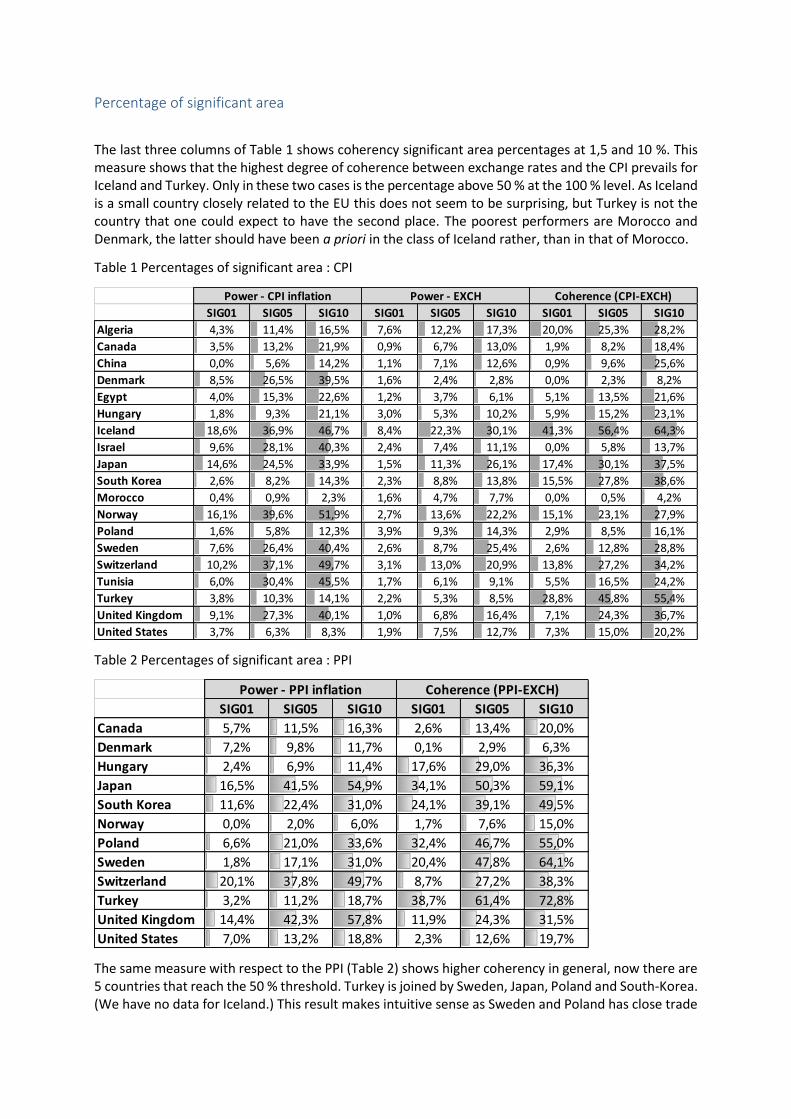
The last three columns of Table 1 shows coherency significant area percentages at 1,5 and 10 %. This measure shows that the highest degree of coherence between exchange rates and the CPI prevails for Iceland and Turkey. Only in these two cases is the percentage above 50 % at the 100 % level. As Iceland is a small country closely related to the EU this does not seem to be surprising, but Turkey is not the country that one could expect to have the second place. The poorest performers are Morocco and Denmark, the latter should have been a priori in the class of Iceland rather, than in that of Morocco.

Table 1 Percentages of significant area : CPI

Table 2 Percentages of significant area : PPI

The same measure with respect to the PPI (Table 2) shows higher coherency in general, now there are 5 countries that reach the 50 % threshold. Turkey is joined by Sweden, Japan, Poland and South-Korea. (We have no data for Iceland.) This result makes intuitive sense as Sweden and Poland has close trade

SIG01 SIG05 SIG10 SIG01 SIG05 SIG10 SIG01 SIG05 SIG10

Algeria 4,3% 11,4% 16,5% 7,6% 12,2% 17,3% 20,0% 25,3% 28,2%

Canada 3,5% 13,2% 21,9% 0,9% 6,7% 13,0% 1,9% 8,2% 18,4%

China 0,0% 5,6% 14,2% 1,1% 7,1% 12,6% 0,9% 9,6% 25,6%

Denmark 8,5% 26,5% 39,5% 1,6% 2,4% 2,8% 0,0% 2,3% 8,2%

Egypt 4,0% 15,3% 22,6% 1,2% 3,7% 6,1% 5,1% 13,5% 21,6%

Hungary 1,8% 9,3% 21,1% 3,0% 5,3% 10,2% 5,9% 15,2% 23,1%

Iceland 18,6% 36,9% 46,7% 8,4% 22,3% 30,1% 41,3% 56,4% 64,3%

Israel 9,6% 28,1% 40,3% 2,4% 7,4% 11,1% 0,0% 5,8% 13,7%

Japan 14,6% 24,5% 33,9% 1,5% 11,3% 26,1% 17,4% 30,1% 37,5%

South Korea 2,6% 8,2% 14,3% 2,3% 8,8% 13,8% 15,5% 27,8% 38,6%

Morocco 0,4% 0,9% 2,3% 1,6% 4,7% 7,7% 0,0% 0,5% 4,2%

Norway 16,1% 39,6% 51,9% 2,7% 13,6% 22,2% 15,1% 23,1% 27,9%

Poland 1,6% 5,8% 12,3% 3,9% 9,3% 14,3% 2,9% 8,5% 16,1%

Sweden 7,6% 26,4% 40,4% 2,6% 8,7% 25,4% 2,6% 12,8% 28,8%

Switzerland 10,2% 37,1% 49,7% 3,1% 13,0% 20,9% 13,8% 27,2% 34,2%

Tunisia 6,0% 30,4% 45,5% 1,7% 6,1% 9,1% 5,5% 16,5% 24,2%

Turkey 3,8% 10,3% 14,1% 2,2% 5,3% 8,5% 28,8% 45,8% 55,4%

United Kingdom 9,1% 27,3% 40,1% 1,0% 6,8% 16,4% 7,1% 24,3% 36,7%

United States 3,7% 6,3% 8,3% 1,9% 7,5% 12,7% 7,3% 15,0% 20,2%

Power - CPI inflation Power - EXCH Coherence (CPI-EXCH)

SIG01 SIG05 SIG10 SIG01 SIG05 SIG10

Canada 5,7% 11,5% 16,3% 2,6% 13,4% 20,0%

Denmark 7,2% 9,8% 11,7% 0,1% 2,9% 6,3%

Hungary 2,4% 6,9% 11,4% 17,6% 29,0% 36,3%

Japan 16,5% 41,5% 54,9% 34,1% 50,3% 59,1%

South Korea 11,6% 22,4% 31,0% 24,1% 39,1% 49,5%

Norway 0,0% 2,0% 6,0% 1,7% 7,6% 15,0%

Poland 6,6% 21,0% 33,6% 32,4% 46,7% 55,0%

Sweden 1,8% 17,1% 31,0% 20,4% 47,8% 64,1%

Switzerland 20,1% 37,8% 49,7% 8,7% 27,2% 38,3%

Turkey 3,2% 11,2% 18,7% 38,7% 61,4% 72,8%

United Kingdom 14,4% 42,3% 57,8% 11,9% 24,3% 31,5%

United States 7,0% 13,2% 18,8% 2,3% 12,6% 19,7%

Power - PPI inflation Coherence (PPI-EXCH)

relationships with Germany, while Japan and South Korea are substantial industrial exporters, and the PPI and export prices have always been found to move more in accordance with exchange rates than consumer prices.

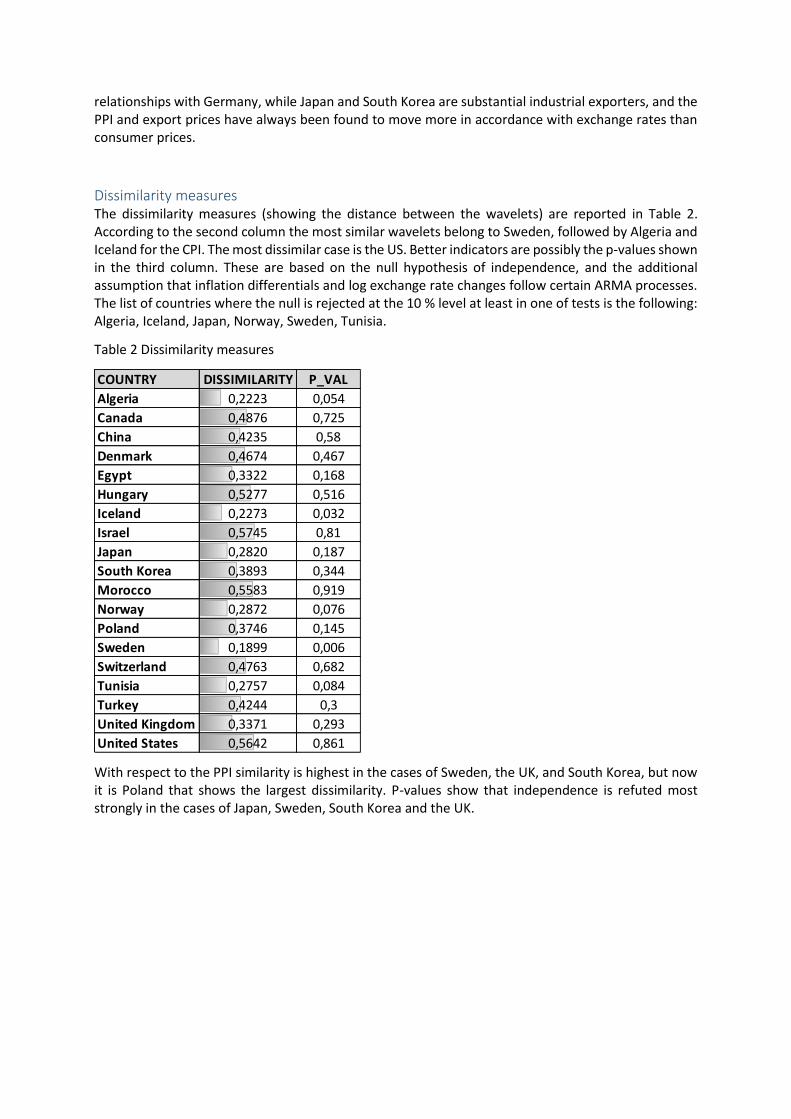
Dissimilarity measures The dissimilarity measures (showing the distance between the wavelets) are reported in Table 2. According to the second column the most similar wavelets belong to Sweden, followed by Algeria and Iceland for the CPI. The most dissimilar case is the US. Better indicators are possibly the p-values shown in the third column. These are based on the null hypothesis of independence, and the additional assumption that inflation differentials and log exchange rate changes follow certain ARMA processes. The list of countries where the null is rejected at the 10 % level at least in one of tests is the following: Algeria, Iceland, Japan, Norway, Sweden, Tunisia.

Table 2 Dissimilarity measures

With respect to the PPI similarity is highest in the cases of Sweden, the UK, and South Korea, but now it is Poland that shows the largest dissimilarity. P-values show that independence is refuted most strongly in the cases of Japan, Sweden, South Korea and the UK.

COUNTRY DISSIMILARITY P_VAL

Algeria 0,2223 0,054

Canada 0,4876 0,725

China 0,4235 0,58

Denmark 0,4674 0,467

Egypt 0,3322 0,168

Hungary 0,5277 0,516

Iceland 0,2273 0,032

Israel 0,5745 0,81

Japan 0,2820 0,187

South Korea 0,3893 0,344

Morocco 0,5583 0,919

Norway 0,2872 0,076

Poland 0,3746 0,145

Sweden 0,1899 0,006

Switzerland 0,4763 0,682

Tunisia 0,2757 0,084

Turkey 0,4244 0,3

United Kingdom 0,3371 0,293

United States 0,5642 0,861

Maximal average coherency: scale3 Regarding the CPI one can see that looking for the scale with maximal average coherency the result is extreme in most cases. When we maximize over frequencies from 1 to 10 years in much more than 50 % of cases the maximum is achieved at either the 1 or 10 years scales. When we restrict maximization to 1 to 6 years, 6 years appears frequently. In the cases where the maximum is achieved at 1 year the overall coherency is rather small. The situation with respect to the PPI is essentially the same. The longer the scale the coherency (if any) seems to be stronger.

Table 3: CPI maximum coherencies

Table 4 PPI maximum coherencies

3 The Appendix visualizes the following tables.

COUNTRY DISSIMILARITY P_VAL

Canada 0,5227 0,772

Denmark 0,4477 0,106

Hungary 0,5783 0,921

Japan 0,2657 0,05

South Korea 0,2268 0,015

Norway 0,5043 0,704

Poland 0,6274 0,92

Sweden 0,2097 0,012

Switzerland 0,4023 0,379

Turkey 0,3615 0,159

United Kingdom 0,2246 0,029

United States 0,5790 0,83

COUNTRY

MAX AVG

COHERENCE

(PERIOD 1-10)

MAX AVG

COHERENCE

(PERIOD 1-6)

MAX AVG

COHERENCE

(TIME)

Algeria 8,69 5,90 1994M02

Canada 9,99 5,90 1991M08

China 9,99 3,58 2007M12

Denmark 1,00 1,00 1992M04

Egypt 4,11 4,11 2017M05

Hungary 9,99 3,20 2004M07

Iceland 9,99 5,90 2009M01

Israel 9,99 1,00 1999M07

Japan 9,99 5,90 2017M05

South Korea 9,99 5,90 1998M05

Morocco 6,23 5,90 2017M05

Norway 6,96 5,90 2017M05

Poland 3,48 3,48 1991M08

Sweden 9,99 1,28 1991M08

Switzerland 9,99 5,90 2011M04

Tunisia 9,99 5,90 1997M04

Turkey 6,23 5,90 1994M06

United Kingdom 9,99 3,89 1997M12

United States 1,00 1,00 1991M08

Maximal average coherency: time One can guess that the time index with the maximum average coherency may be around 2008, as it is frequently thought that the connection between exchange rates and prices may strengthen when significant shocks hit the economy. In fact, concerning the CPI nothing similar is observable in our statistics. The most common date is 1991-1992, but this can be due to the fact that these observations are on the edge of our series. However, if we look at the PPI figures, there 2008 seems to be a more prominent time. Of the 12 countries 5 had the highest average coherency either in 2008 or in 2009.

4 Conclusions In this paper we investigated the relationship between the nominal exchange rate and international relative prices, taking Germany as the country of reference. Our methodology was based on the wavelet and cross-wavelet transforms that posit weaker requirements on the data generating process than traditional time-domain methodologies. Our results are in, some ways, accordance with former findings, but suggest an even gloomier view on the possibility of finding statistically solid relationships between exchange rates and aggregate price indices (CPI or PPI). In line with the literature we haven’t found strong co-movement between prices and exchange rates in the short or medium term, and though coherence seems to be increasing with time scale, it seems far from being stable. For instance, we haven’t found any perceivable relationship with respect to Denmark, a country that a priori must have strong connection with Germany. There are weak indications that at least in some countries the price-exchange rate nexus strengthened during the crisis, but even this finding is rather partial and uncertain. In any case detectable cycles at business cycle frequencies do not appear at all. Though by and large the lead-lag relationship between prices and exchange rates is the expected one, still this is unstable practically for every country, to provide a basis for reliable forecasting. As we have expected results with respect to the PPI are more promising, but very similar features could be observed as in the case of the CPI. The three countries that seem to be closest to theoretical expectations are Sweden, Japan and South-Korea, where the first should be one of the foremost candidates for this position, while the latter two not. Indeed, this may indicate that the coherence between exchange rates and prices on the macro level may depend more on similarities of export

COUNTRY

MAX AVG

COHERENCE

(PERIOD 1-10)

MAX AVG

COHERENCE

(PERIOD 1-6)

MAX AVG

COHERENCE

(TIME)

Canada 1,00 1,00 2012M12

Denmark 5,90 5,90 2008M11

Hungary 9,99 4,59 2009M02

Japan 9,99 5,90 1998M05

South Korea 9,99 5,90 1997M05

Norway 6,41 5,90 2008M06

Poland 9,99 5,90 2009M03

Sweden 8,46 5,90 1991M08

Switzerland 9,99 5,90 2014M10

Turkey 9,99 5,90 1994M06

United Kingdom 9,99 5,74 1991M11

United States 9,99 5,90 2008M06

structure than on trading relations, that the microeconomic intuition would suggest. Also, it is possible that macro price indices are too noisy by their very nature to be amenable for statistical analyses not relying on strong presumptions.

5 Literature Aguiar-Conraria, Luís, and Maria Joana Soares. "Oil and the macroeconomy: using wavelets

to analyze old issues." Empirical Economics 40.3 (2011): 645-655.

Bordo, Michael D., Bordo, M. D., Choudhri, E. U., Fazio, G., & MacDonald, R. "The real exchange

rate in the long run: Balassa-Samuelson effects reconsidered." Journal of International Money

and Finance 75 (2017): 69-92.

Burstein, Ariel, and Gita Gopinath. "International prices and exchange rates." Handbook of

international economics. Vol. 4. Elsevier, 2014. 391-451.

Égert, Balázs, László Halpern, and Ronald MacDonald. "Equilibrium exchange rates in

transition economies: taking stock of the issues." Journal of Economic surveys 20.2 (2006):

257-324.

Goupillaud, Pierre, Alex Grossmann, and Jean Morlet. "Cycle-octave and related transforms

in seismic signal analysis." Geoexploration 23.1 (1984): 85-102.

Harris, Fredric J. "On the use of windows for harmonic analysis with the discrete Fourier

transform." Proceedings of the IEEE66.1 (1978): 51-83.

Kumar, Praveen, and Efi Foufoula-Georgiou. "Wavelet analysis in geophysics: An

introduction." Wavelets in geophysics 4 (1994): 1-43.

Soares, Maria Joana, and Luís Aguiar-Conraria. "Inflation Rate Dynamics Convergence

within the Euro." International Conference on Computational Science and Its Applications.

Springer, Cham, 2014.

Taylor, Alan M., and Mark P. Taylor. "The purchasing power parity debate." Journal of

economic perspectives 18.4 (2004): 135-158.

Torrence, Christopher, and Gilbert P. Compo. "A practical guide to wavelet

analysis." Bulletin of the American Meteorological society 79.1 (1998): 61-78.

Appendix: Wavelet Power Figures

Algeria

Canada

China

Denmark

Egypt

HungaryIcelandIsrael

Japan

South_Korea

Morocco

Norway

Poland

Sweden

Switzerland

Tunisia

Turkey

United_Kingdom

United_States

0

2

4

6

8

10

12

1988 1993 1998 2003 2008 2013 2018

Period (in years) with maximum average coherence vs. time (month) with maximum average coherence (CPI-EXCH)

AlgeriaCanada

China

Denmark

Egypt

Hungary

Iceland

IsraelJapan

South_KoreaMorocco

Norway

Poland

Sweden

Switzerland

Tunisia

Turkey

United_Kingdom

United_States

0

1

2

3

4

5

6

7

1988 1993 1998 2003 2008 2013 2018

Period (in years) with maximum average power vs. time (month) with maximum average power (CPI)

AlgeriaCanada

China

Denmark

Egypt

Hungary

Iceland

IsraelJapan

South_KoreaMorocco

Norway

Poland

Sweden

Switzerland

Tunisia

Turkey

United_Kingdom

United_States

0,0

0,5

1,0

1,5

2,0

2,5

3,0

1988 1993 1998 2003 2008 2013 2018

Period (in years) with maximum average power vs. time (month) with maximum average power (EXCH)

Canada

Denmark

Hungary

Japan

South_Korea

Norway

Poland

Sweden

Switzerland

Turkey

United_KingdomUnited_States

0

2

4

6

8

10

12

1988 1993 1998 2003 2008 2013 2018

Period (in years) with maximum average coherence vs. time (month) with maximum average coherence (PPI-EXCH)

Canada

Denmark

Hungary

Japan

South_KoreaNorway

Poland

Sweden

Switzerland

Turkey

United_Kingdom

United_States

0,0

0,5

1,0

1,5

2,0

2,5

3,0

1993 1998 2003 2008 2013 2018

Period (in years) with maximum average power vs. time (month) with maximum average power (PPI)

FIGURES -> Wavelet power (CPI)

FIGURES -> Wavelet power (PPI)

FIGURES -> Wavelet power (EXCH)