EXCHANGE VELOCITY APPROACH AND OBT FORMATION IN PLANTS DURING THE DAYTIME

Anca Melintescu PhD

“Horia Hulubei” National Institute of Physics and Nuclear Engineering, Bucharest - Magurele, ROMANIA

ancameli@ifin.nipne.ro, melianca@yahoo.com

Third Technical Meeting of the EMRAS II, Working Group 7, “Tritium” Accidents, Vienna, Austria, 24 - 28 January 2011

THE DRIVING EQUATIONS FOR TRITIUM TRANSFER IN ATMOSPHERE - SOIL- PLANT CONTINUUM

Driving equation for the HTO transfer from atmosphere to leaves:

ssw

excsair

w

exc CMVCC

MV

dtdC )()91.0(

C – HTO concentration in plant water (Bq/kg); Cair – HTO concentration in air (Bq/m3); Cs - HTO concentration in the sap water (Bq/kg); s - saturated air humidity at vegetation temp. (kg/m3); - air humidity at reference level (kg/m3); Mw – water mass in plant on a unit soil surface (kg/m2); Vexc – exchange velocity from atmosphere to canopy (m/s)

the transpiration flux - used for all canopy, ignoring the transfer of air HTO to steam, because the exchange velocity is smaller with one order of magnitude;- Ignores the initial diffusion of leaf water to steams

The tritium dynamics at soil surface:

DFCTCMV

dtdC

swssatairws

sexsw ))(91.0( 1,,1, Csw,1 - HTO concentration in the first soil layer at the (Bq/kg);

Vex,s - exchange velocity from atmosphere to soil (m/s); sat(Ts) - saturated air humidity at soil surface temp. (kg/m3); Mws – water mass in the surface soil layer; DF - HTO net flux at the bottom interface of the first soil layer

depends on canopy resistance

depends on soil resistance

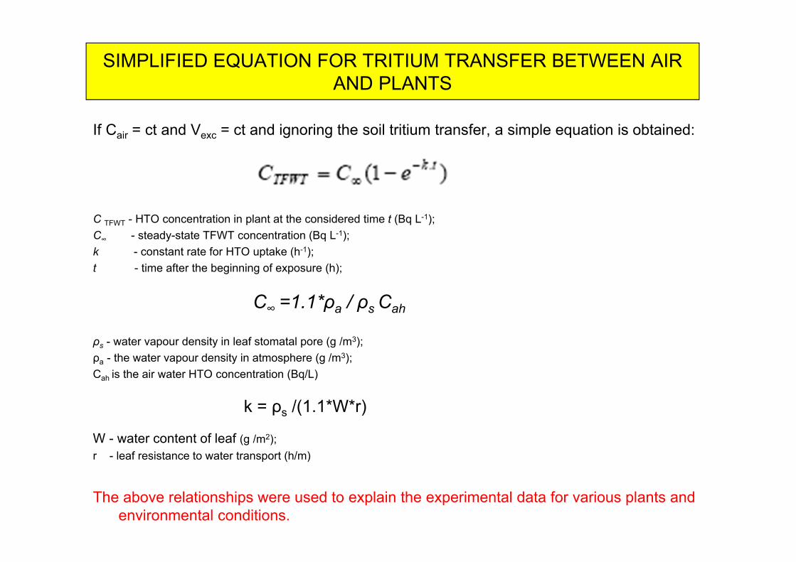
SIMPLIFIED EQUATION FOR TRITIUM TRANSFER BETWEEN AIR AND PLANTS

If Cair = ct and Vexc = ct and ignoring the soil tritium transfer, a simple equation is obtained:

C TFWT - HTO concentration in plant at the considered time t (Bq L-1);C∞ - steady-state TFWT concentration (Bq L-1);k - constant rate for HTO uptake (h-1);t - time after the beginning of exposure (h);

C∞ =1.1*ρa / ρs Cah

ρs - water vapour density in leaf stomatal pore (g /m3);ρa - the water vapour density in atmosphere (g /m3); Cah is the air water HTO concentration (Bq/L)

k = ρs /(1.1*W*r)

W - water content of leaf (g /m2); r - leaf resistance to water transport (h/m)

The above relationships were used to explain the experimental data for various plants and environmental conditions.

M. Andoh Atarashi et al., 1997

Large variability between plants and environmental conditions → Need to consider the variability of exchange velocity

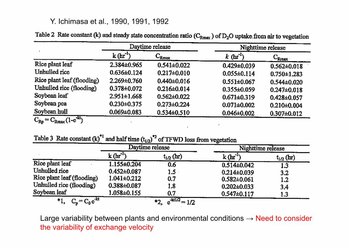
Y. Ichimasa et al., 1990, 1991, 1992

Large variability between plants and environmental conditions → Need to consider the variability of exchange velocity

Resistance Approaches for Deposition and Exchange• Similitude between water vapour transport

and electric circuits → in both cases the transport is due to specific gradients:

- specific humidity for water- electric potential for electricity

• Environmental resistances - analogy with electric resistances → both = the ratio between potential difference and flux

• Ra - turbulence and wind speed

• Rb - turbulence, wind speed and surface properties

• Total surface resistance Rc - split up into canopy and ground related resistance

• Canopy resistance - surface properties, temperature, PAR, humidity, water content in soil

• HT deposition → ground resistance depends on the rates of diffusion and oxidation in soil;

- much lower than the canopy resistance

Atmospheric source

Aerodynamic, Ra

Boundary, Rb

Stomatal, Rs

Cuticular, Rct

Ground, Rg

for various surfacesTo

tal S

urfa

ce, R

c

exchange velocity at air to plant (soil) interface

cbaex RRR

V

1

↓

Visualization of momentum transfer

Turbulent eddies - responsible for transporting material through the surface boundary layer

Transport processes:

- transfer of heat- mass - momentum

Distinct aspect of the boundary layer → turbulent nature

A force is needed to change momentum transfer from one level to another. This drag force or shear stress is also equivalent to the momentum flux densityMomentum must be transferred downward.

u* - friction velocityK – von Karmann’s constant (=0.40)z - height above the groundz0 – roughness parameter = the effectiveness of a canopy to absorb momentum; valid only for very short vegetation and for a neutrally stratified atmosphered - Zero-Plane Displacement Height = the level at which surface drag acts on the roughness elements or level which would be obtained by flattening out all the roughness elements into a smooth surface.

Logarithmic wind profile:

Boundary layer

modify the atmosphere’s properties

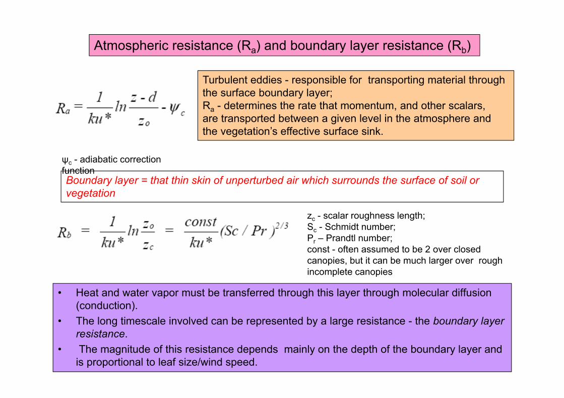
• Heat and water vapor must be transferred through this layer through molecular diffusion (conduction).

• The long timescale involved can be represented by a large resistance - the boundary layer resistance.

• The magnitude of this resistance depends mainly on the depth of the boundary layer and is proportional to leaf size/wind speed.

Atmospheric resistance (Ra) and boundary layer resistance (Rb)

Turbulent eddies - responsible for transporting material through the surface boundary layer; Ra - determines the rate that momentum, and other scalars, are transported between a given level in the atmosphere and the vegetation’s effective surface sink.

ψc - adiabatic correction functionBoundary layer = that thin skin of unperturbed air which surrounds the surface of soil or vegetation

zc - scalar roughness length; Sc - Schmidt number; Pr – Prandtl number;const - often assumed to be 2 over closed canopies, but it can be much larger over rough incomplete canopies

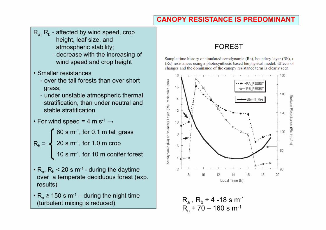
Ra, Rb - affected by wind speed, crop height, leaf size, and atmospheric stability;

- decrease with the increasing of wind speed and crop height

• Smaller resistances - over the tall forests than over short

grass; - under unstable atmospheric thermal

stratification, than under neutral and stable stratification

• For wind speed = 4 m s-1 →

Rb =

• Ra, Rb < 20 s m-1 - during the daytime over a temperate deciduous forest (exp. results)

• Ra ≥ 150 s m-1 – during the night time (turbulent mixing is reduced) Ra , Rb ÷ 4 -18 s m-1

Rc ÷ 70 – 160 s m-1

FOREST

60 s m-1, for 0.1 m tall grass

20 s m-1, for 1.0 m crop

10 s m-1, for 10 m conifer forest

CANOPY RESISTANCE IS PREDOMINANT

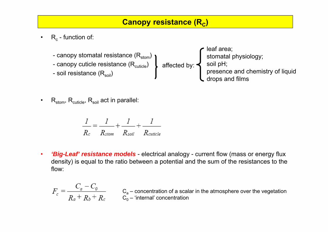
Canopy resistance (RC)

• Rc - function of:

- canopy stomatal resistance (Rstom)- canopy cuticle resistance (Rcuticle)- soil resistance (Rsoil)

• Rstom, Rcuticle, Rsoil act in parallel:

• ‘Big-Leaf’ resistance models - electrical analogy - current flow (mass or energy flux density) is equal to the ratio between a potential and the sum of the resistances to the flow:

Ca – concentration of a scalar in the atmosphere over the vegetationC0 – ‘internal’ concentration

affected by:

leaf area;stomatal physiology;soil pH;presence and chemistry of liquiddrops and films

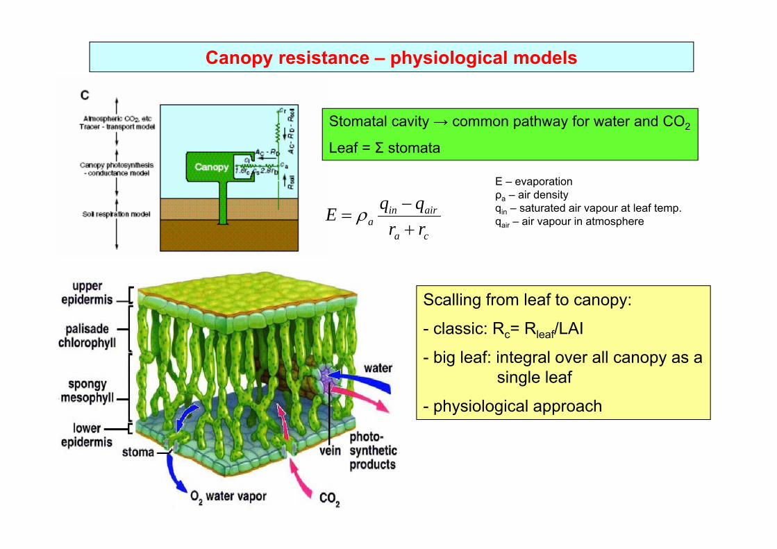
Stomatal cavity → common pathway for water and CO2

Leaf = Σ stomata

Scalling from leaf to canopy:

- classic: Rc= Rleaf/LAI

- big leaf: integral over all canopy as asingle leaf

- physiological approach

ca

airina rr

qqE

E – evaporationρa – air densityqin – saturated air vapour at leaf temp.qair – air vapour in atmosphere

Canopy resistance – physiological models

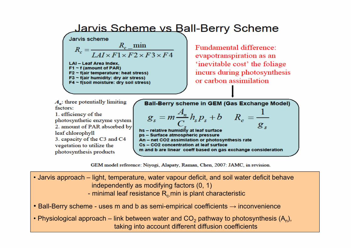
• Jarvis approach – light, temperature, water vapour deficit, and soil water deficit behaveindependently as modifying factors (0, 1)

- minimal leaf resistance Rc-min is plant characteristic

• Ball-Berry scheme - uses m and b as semi-empirical coefficients → inconvenience

• Physiological approach – link between water and CO2 pathway to photosynthesis (An), taking into account different diffusion coefficients

Physiological approach (preferred and tested)

gmin,c - the cuticular conductanceAg - the gross assimilation rate of leafDs - the vapour pressure deficit at plant levelCs - the CO2 concentration at the leaf surfaceCi - the CO2 concentration in the plant interiorf 0 - the maximum value of (Ci - Γ )/(Cs - Γ)fmin - the minimum value of (Ci - Γ )/(Cs - Γ)D0 - the value of Ds at which the stomata are closedΓ – CO2 compensation point

• For canopy - integrate on LAI• We use gross canopy photosynthesis rate from WOFOST• Data base exist → advantage

gl,c – leaf C conductance;gl,w– leaf water conductance;gc,c– C canopy conductance;gc,w- water canopy conductance

- assumes that C conductance is determined by ratio between photosynthetic rate and the concentration difference of CO2 for leaf surface and leaf interior

(Jacobs - Calvet)

0

0.2

0.4

0.6

0.8

1

1.2

0 0.5 1 1.5 2 2.5 3

VPD (kPa])

Rela

tive

cond

ucta

nce

C3 teoDo=0.7 Do=1Do=1.5

Vegetation type fo ad (kPa-1)

Low vegetation C3 0.89 0.07

Low vegetation C4 0.85 0.015

Lobos 0.093 0.12

Rice and phalaris grass 0.89 0.18

Forest temperate 0.875 0.06

Boreal forest 0.4 0.12

Water vapour deficit

Stomatal conductance and humidity deficit - C3 and C4 plants

00.0020.0040.0060.0080.01

0.0120.0140.0160.018

0 5 10 15 20

Humidity deficit (g/kg)

Stom

atal

con

duct

ance

(m/s

)g_C3g_C4

Ronda approach- simplifies Jacobs – Calvet approach:

f0, ad – empirically found asregression coefficientsD0 – vapour pressure deficit forwhich stomata are closed

- light, temperature, VPD, soil water deficit - environmental factors influencing the canopy resistance

Soil water deficit

Ag - the gross assimilation rate of leaf- the unstressed assimilation (mol m-2s-1) rate

- the average soil water content in root zoneWP - the wilting point FC - the field capacityΘi - mean soil moisture in “i” layerRi - root fraction in “i” layer

*gA

_

- CO2 assimilation rate - seriously affected by soil water stress, especially during the summer time → the water supply is low

↓correction factor for water stress

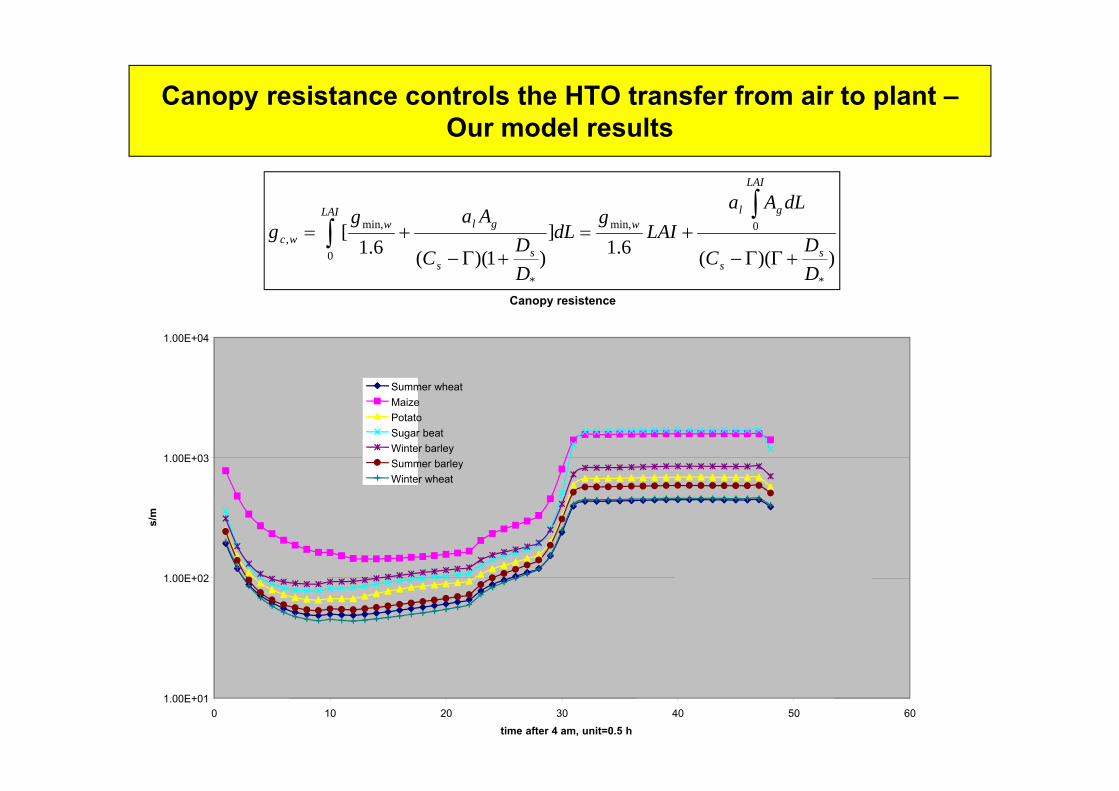
LAI

ss

LAI

glw

ss

glwwc

DD

C

dLAaLAI

gdL

DD

C

Aagg

0

*

0min,

*

min,,

))((6.1]

)1)((6.1[

Canopy resistance controls the HTO transfer from air to plant –Our model results

Canopy resistence

1.00E+01

1.00E+02

1.00E+03

1.00E+04

0 10 20 30 40 50 60time after 4 am, unit=0.5 h

s/m

Summer wheatMaize Potato Sugar beatWinter barleySummer barleyWinter wheat

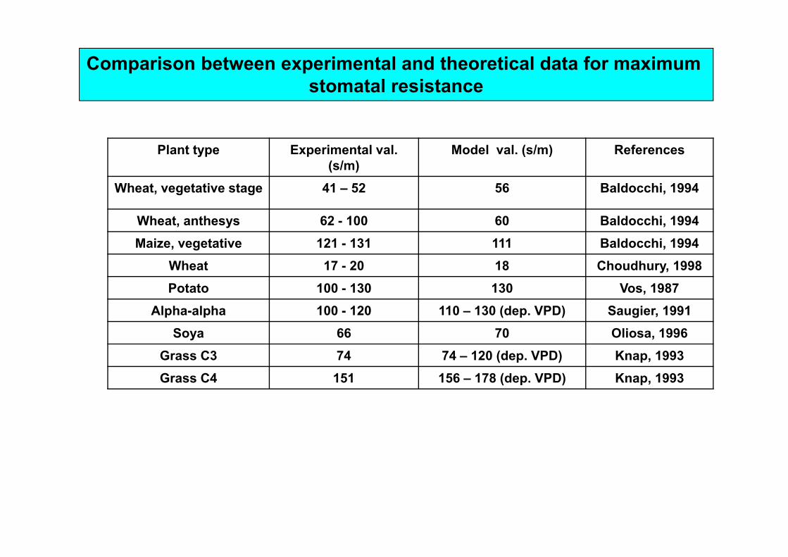
Comparison between experimental and theoretical data for maximum stomatal resistance

Plant type Experimental val. (s/m)

Model val. (s/m) References

Wheat, vegetative stage 41 – 52 56 Baldocchi, 1994

Wheat, anthesys 62 - 100 60 Baldocchi, 1994Maize, vegetative 121 - 131 111 Baldocchi, 1994

Wheat 17 - 20 18 Choudhury, 1998Potato 100 - 130 130 Vos, 1987

Alpha-alpha 100 - 120 110 – 130 (dep. VPD) Saugier, 1991Soya 66 70 Oliosa, 1996

Grass C3 74 74 – 120 (dep. VPD) Knap, 1993Grass C4 151 156 – 178 (dep. VPD) Knap, 1993

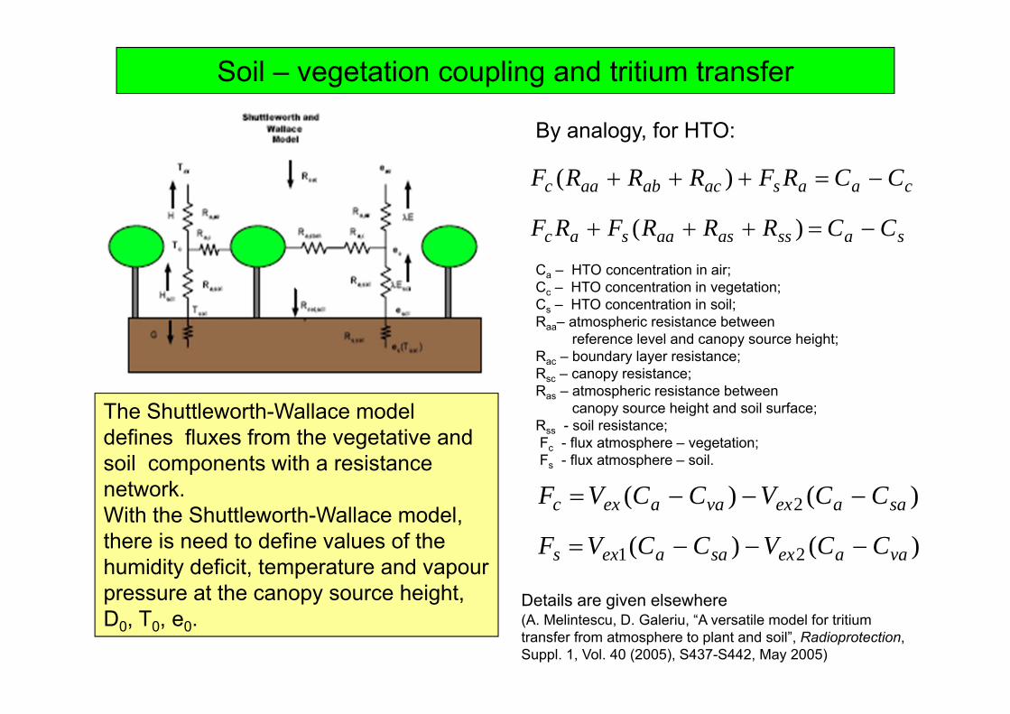
Soil – vegetation coupling and tritium transfer

The Shuttleworth-Wallace model defines fluxes from the vegetative and soil components with a resistance network. With the Shuttleworth-Wallace model, there is need to define values of the humidity deficit, temperature and vapour pressure at the canopy source height, D0, T0, e0.

caasacabaac CCRFRRRF )(

sassasaasac CCRRRFRF )(

By analogy, for HTO:

Ca – HTO concentration in air; Cc – HTO concentration in vegetation;Cs – HTO concentration in soil;Raa– atmospheric resistance between

reference level and canopy source height;Rac – boundary layer resistance;Rsc – canopy resistance; Ras – atmospheric resistance between

canopy source height and soil surface;Rss - soil resistance;Fc - flux atmosphere – vegetation;Fs - flux atmosphere – soil.

)()( 2 saaexvaaexc CCVCCVF

)()( 21 vaaexsaaexs CCVCCVF

Details are given elsewhere(A. Melintescu, D. Galeriu, “A versatile model for tritium transfer from atmosphere to plant and soil”, Radioprotection,Suppl. 1, Vol. 40 (2005), S437-S442, May 2005)

1.E+02

1.E+03

1.E+04

1.E+05

1.E+06

1.E+07

1.E+08

0 20 40 60 80 100

time h

Cve

g B

q/L

LAI=5;dry

LAI=5;w et

LAI=1;w et

Lai=1;dry

HTO concentration in vegetation in the sparse canopy approach

Coupling between soil surface and vegetation layer has a significant influence on canopy HTO concentration at both low and high Leaf Area Index → more studies are justified.

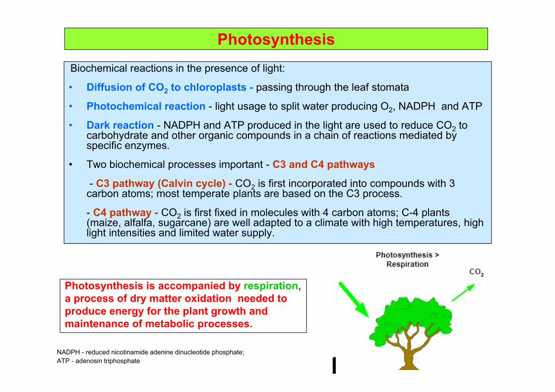
PhotosynthesisBiochemical reactions in the presence of light:

• Diffusion of CO2 to chloroplasts - passing through the leaf stomata

• Photochemical reaction - light usage to split water producing O2, NADPH and ATP

• Dark reaction - NADPH and ATP produced in the light are used to reduce CO2 to carbohydrate and other organic compounds in a chain of reactions mediated by specific enzymes.

• Two biochemical processes important - C3 and C4 pathways

- C3 pathway (Calvin cycle) - CO2 is first incorporated into compounds with 3 carbon atoms; most temperate plants are based on the C3 process.

- C4 pathway - CO2 is first fixed in molecules with 4 carbon atoms; C-4 plants (maize, alfalfa, sugarcane) are well adapted to a climate with high temperatures, high light intensities and limited water supply.

Photosynthesis is accompanied by respiration,a process of dry matter oxidation needed to produce energy for the plant growth and maintenance of metabolic processes.

NADPH - reduced nicotinamide adenine dinucleotide phosphate; ATP - adenosin triphosphate

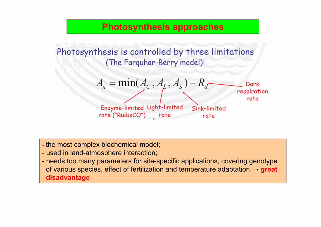
Photosynthesis approaches

- the most complex biochemical model; - used in land-atmosphere interaction;- needs too many parameters for site-specific applications, covering genotype

of various species, effect of fertilization and temperature adaptation → great disadvantage

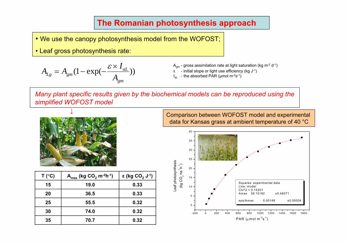
The Romanian photosynthesis approach

• We use the canopy photosynthesis model from the WOFOST;

• Leaf gross photosynthesis rate:

))exp(1(gm

aLgmLg A

IAA Agm - gross assimilation rate at light saturation (kg m-2 d-1)

ε - initial slope or light use efficiency (kg J-1)IaL - the absorbed PAR (μmol m-2s-1)

Many plant specific results given by the biochemical models can be reproduced using the simplified WOFOST model

T (°C) Amax (kg CO2 m-2h-1) ε (kg CO2 J-1)

15 19.0 0.33

20 36.5 0.33

25 55.5 0.32

30 74.0 0.32

35 70.7 0.32-200 0 200 400 600 800 1000 1200 1400 1600 1800

0

5

10

15

20

25

30

35

40

Squares: experimental data Line: modelChi^2 = 0.15201Amax 39.15192 ±0.46071

eps/Amax 0.00148 ±0.00004

Leaf

pho

tosy

nthe

sis

(kg

CO

2 ha-1

h-1)

PAR (m ol m -2s-1)

Comparison between WOFOST model and experimental data for Kansas grass at ambient temperature of 40 °C

↓

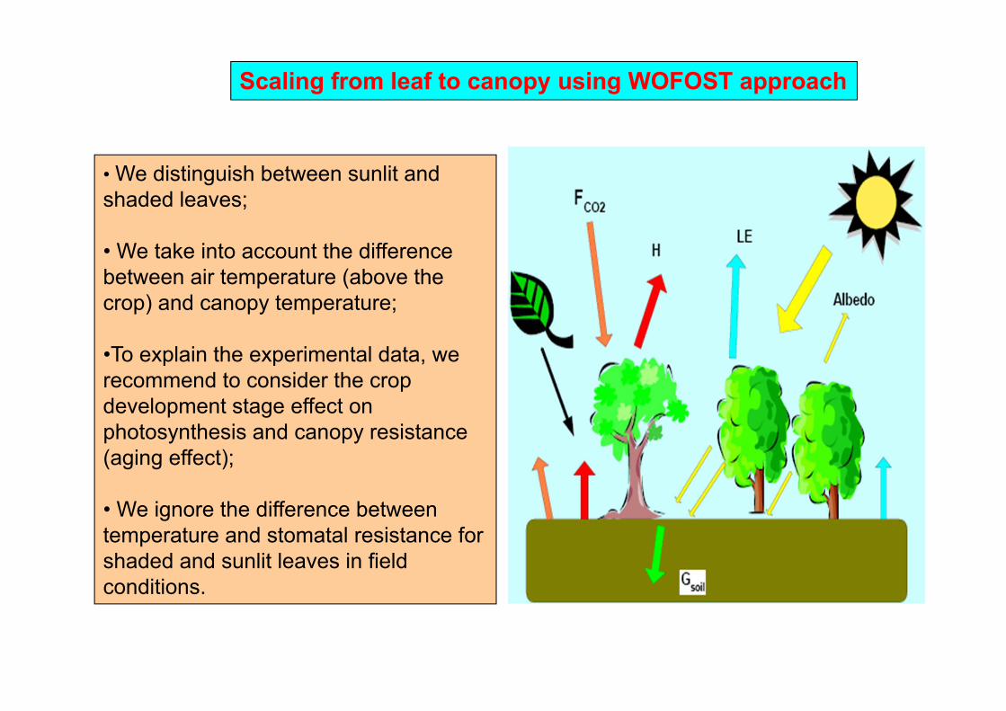
• We distinguish between sunlit and shaded leaves;

• We take into account the difference between air temperature (above the crop) and canopy temperature;

•To explain the experimental data, we recommend to consider the crop development stage effect on photosynthesis and canopy resistance (aging effect);

• We ignore the difference between temperature and stomatal resistance for shaded and sunlit leaves in field conditions.

Scaling from leaf to canopy using WOFOST approach

OBT production in the daytime

• In the simplest approach, we ignore details on respiration and focus on net photosynthesis rate (net of respiration).

• Assume that we know the net assimilation rate of CO2 as kg CO2 per unit time and unit surface of crop, Pc.

• One mol of CO2 and one mol of H2O gives one mol of photosinthate (the initial organic matter produced), with a generic formula CH2O.

• The rate of water assimilation in non-exchangeable matter (bound with C) can be obtained using stoichiometric relations (molar mass of CO2 is 44, molar mass of H2O is 18) and is 0.41 PC.

• Consider tritium, as tritiated water → due to higher mass, all reactions rates will be slower.

• Energy of radioactive disintegration (average 5.8 keV) will be used partially for the activation energy of many biochemical reactions.

• Plant varies in their molecular constituent → the balance of slow down and acceleration of biochemical reaction is reflected in a variable fractionation (discrimination) ratio, FD (formation of OBT/formation of OBH), with an average of 0.5 and range between 0.45 and 0.55.

With a known CHTO in leaves, we can assess the formation rate of OBT in lightconditions:

POBT = FD*0.41*Pc* CHTO (Bq/h/m2) → we must use the HTO in leaves, because leaves are the site of photosynthesis

In the same conditions of time and space, the net dry matter production is:

Total organic tritium is higher, because about 22 % is non-exchangeable:

POBT = 0.88*POT

In practice, the leaf HTO concentration varies in time → Pc varies, also (with zeroduring the night time)

CD PP4430

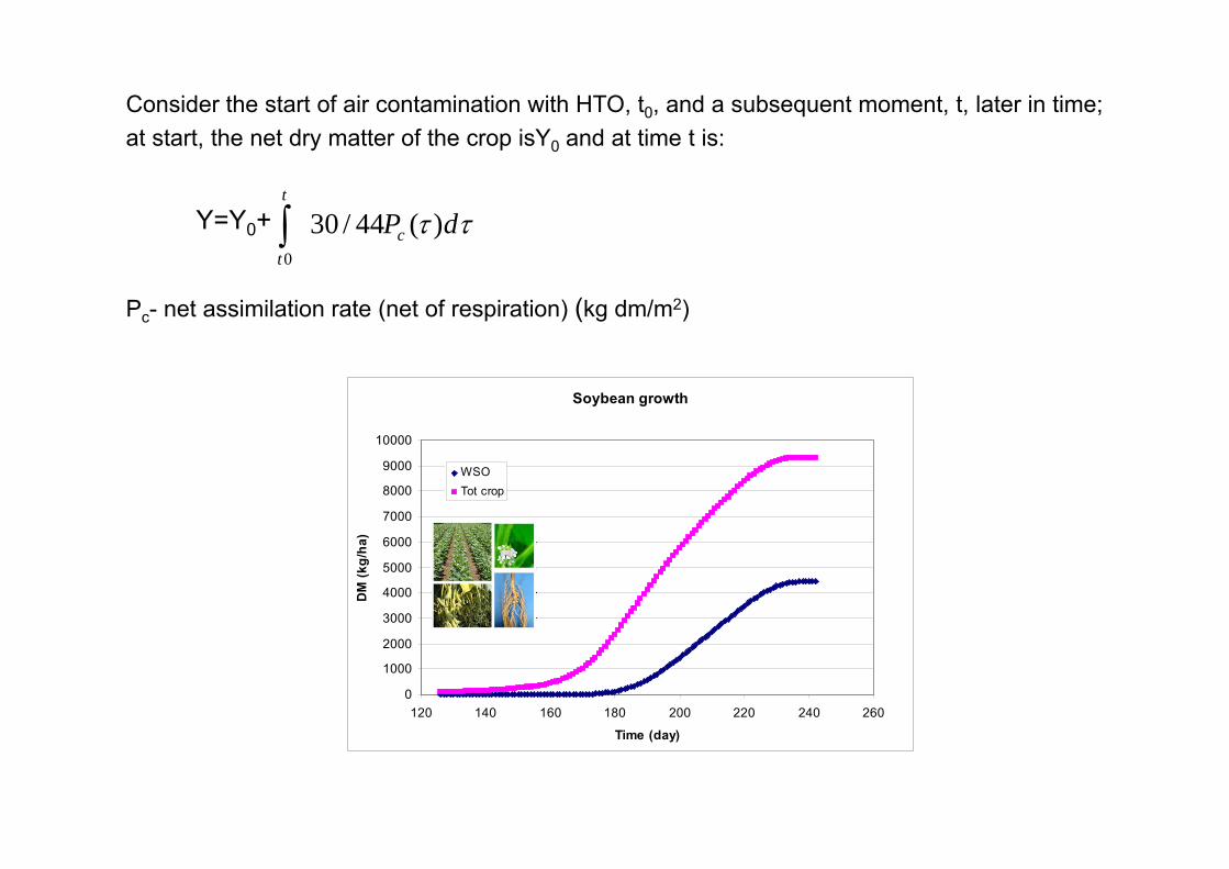
Soybean growth

0

1000

2000

3000

4000

5000

6000

7000

8000

9000

10000

120 140 160 180 200 220 240 260

Time (day)

DM

(kg/

ha)

WSOTot crop

Consider the start of air contamination with HTO, t0, and a subsequent moment, t, later in time; at start, the net dry matter of the crop isY0 and at time t is:

Y=Y0+ dPc

t

t

)(44/300

Pc- net assimilation rate (net of respiration) (kg dm/m2)

• If we ignore OBT production during the night time, we can derive a similar equation of OBT production for the whole crop.

• The evolution of OBT concentration COBT (Bq/kg dm) is of interest in food chain modelling.

• First, we consider the concentration in whole crop (including roots); we have:

where:

DOBT

OBTOBT P

YC

PYdt

dC*)(*)1(

cOBT

HTOcOBT P

YC

CPFDYdt

dC*68.0*)(***41.0*)1(

YCA OBTOBT dtdYC

dtdCY

dtdA **

dtdYC

dtdCYPOBT **

DOBT

HTODOBT P

YCCPFD

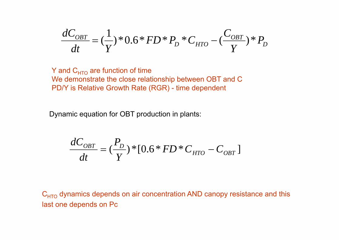
YdtdC *)(***6.0*)1(

Y and CHTO are function of time We demonstrate the close relationship between OBT and CPD/Y is Relative Growth Rate (RGR) - time dependent

]**6.0[*)( OBTHTODOBT CCFD

YP

dtdC

CHTO dynamics depends on air concentration AND canopy resistance and this last one depends on Pc

Dynamic equation for OBT production in plants:

OBT concentration in edible plant parts (net of respiration)

0.0E+00

5.0E+011.0E+02

1.5E+02

2.0E+02

2.5E+023.0E+02

3.5E+02

4.0E+02

0 50 100 150

days after sowing

conc

entra

tion,

at h

arve

st

steemleavesshellseeds

OBT concentration for soybean at harvest for 1 hour air contamination at various plant DVS

Partition fraction of new produced dry matter to roots, leaves, stems and edible grains as function of DVS (0=emergence; 1= flowering; 2= full maturity) for maize cultivar F320 (South Romania)

• At each stage of plant development, the new formed net dry matter will be differently distributed to various plant parts → initial uptake and time evolution depends on plant part.

• We must know these partition factors in order to assess OBT in the edible plant part.

• Even for leafy vegetables and pasture, we must know the partition to root.

00.10.20.30.40.50.60.70.80.9

1

0 0.5 1 1.5 2DVS

part

ition

frac

tion

Rootsleavessteamsgrain

• PARTITION FACTORS DEPEND ON CULTIVAR (GENOTYPE), not only on PLANT

• Pc depends on:- crop type; - development stage (DVS);- leaf area index (LAI);- temperature;- light;- water stress (air vapour deficit and soil water)

• We must understand the plant growth

• Development stages:

0 -1 - emergence to anthesis (flowering) → generative stage1 -2 - anthesis to maturity → reproductive stage both can be finer divided

• Evolution of plant development depends on Thermal time = sum of air temperature over a basis

OBT concentration in different plant parts

• At least, we must know crop specific accumulated thermal time until anthesis and maturity → we can define the increasing of DVS each day → partition factors → increase in leaf mass → green leaves → LAI

• Knowing the ambient data on temperature, light, vapour pressure and soil water, we can determine PC, PD, POBT

OBT concentration in plant part i

Partition fraction PFi (DVS) → PFi(t)

PD,i=PD*PFiPOBT,i= POBT* PFi

iDi

iOBTiOBT

i

iOBT PY

CP

YdtdC

i

,,

,, *)(*)1(

Time Rel. OBT conc. at harvest (%) Exposure conditionsExp. Model Solar radiat. (W m-

2)Temp. (°C)

Dawn 0.18 0.29 90-170 11-26

Day 0.25 0.34 400-800 26-36

Dusk 0.20 0.34 26-38 15-24

Night 0.15 0.31 0 12-17

Comparison between experimental data and model predictions for relative OBT concentration in wheat at harvest

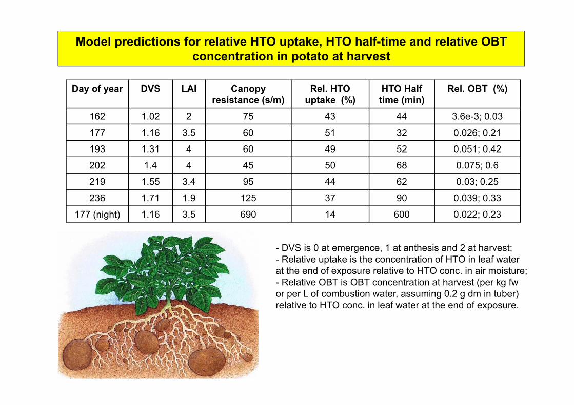
Model predictions for relative HTO uptake, HTO half-time and relative OBT concentration in potato at harvest

Day of year DVS LAI Canopy resistance (s/m)

Rel. HTO uptake (%)

HTO Half time (min)

Rel. OBT (%)

162 1.02 2 75 43 44 3.6e-3; 0.03

177 1.16 3.5 60 51 32 0.026; 0.21

193 1.31 4 60 49 52 0.051; 0.42

202 1.4 4 45 50 68 0.075; 0.6

219 1.55 3.4 95 44 62 0.03; 0.25

236 1.71 1.9 125 37 90 0.039; 0.33

177 (night) 1.16 3.5 690 14 600 0.022; 0.23

- DVS is 0 at emergence, 1 at anthesis and 2 at harvest;- Relative uptake is the concentration of HTO in leaf water at the end of exposure relative to HTO conc. in air moisture;- Relative OBT is OBT concentration at harvest (per kg fw or per L of combustion water, assuming 0.2 g dm in tuber) relative to HTO conc. in leaf water at the end of exposure.

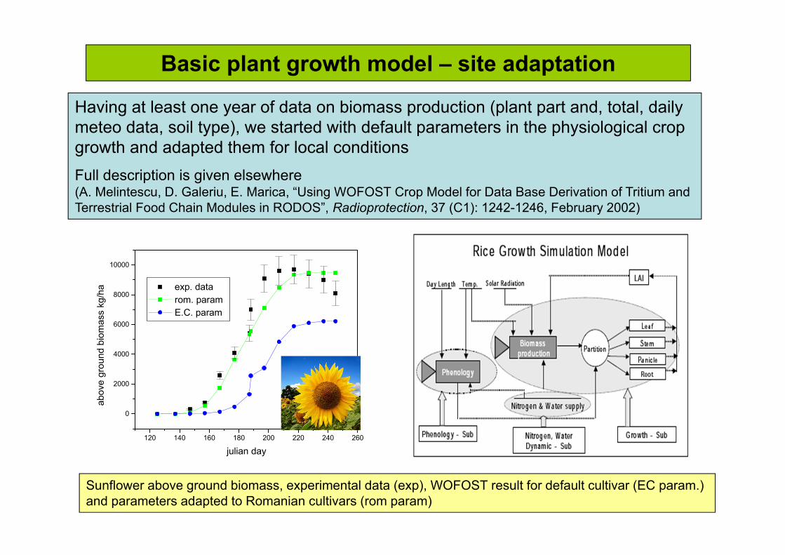
Basic plant growth model – site adaptation

120 140 160 180 200 220 240 260

0

2000

4000

6000

8000

10000

exp. data rom. param E.C. param

abov

e gr

ound

bio

mas

s kg

/ha

julian day

Having at least one year of data on biomass production (plant part and, total, daily meteo data, soil type), we started with default parameters in the physiological crop growth and adapted them for local conditionsFull description is given elsewhere(A. Melintescu, D. Galeriu, E. Marica, “Using WOFOST Crop Model for Data Base Derivation of Tritium and Terrestrial Food Chain Modules in RODOS”, Radioprotection, 37 (C1): 1242-1246, February 2002)

Sunflower above ground biomass, experimental data (exp), WOFOST result for default cultivar (EC param.) and parameters adapted to Romanian cultivars (rom param)

Role of respiration in OBT formation

• Respiration is often subdivided into:- Growth;- Maintenance;- Transport costs.

Growth respiration (a.k.a. “construction respiration”) – a “fixed cost” that depends on the tissues or biochemical's that are synthesized → Often described in terms of “glucose equivalents”

• The conversion of assimilate into dry matter (growth respiration) can be counted first converting the CO2 assimilation to assimilate production (30/44) and further considering the conversion from assimilate top dry matter depending also on plant stage

• In vegetative period (only leaves, roots and stems) a value of 0.69 is OK (coefficient of variance less than 5%).

• In reproductive stage the same value can be used, but with a larger variance.

• Storage organs for different plants have:- soybean - 0.48; - field bean - 0.59; - sugar beat - 0.82; - potato - 0.85

It seems that growth respiration ends the next morning!

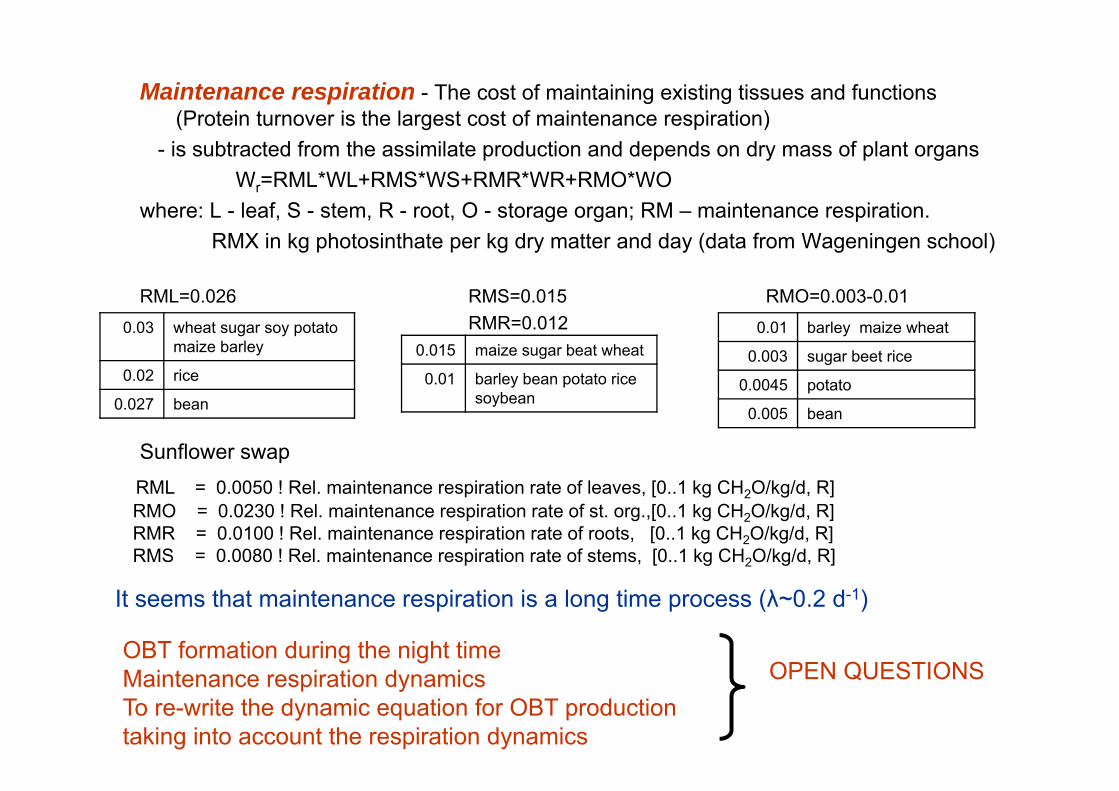
Maintenance respiration - The cost of maintaining existing tissues and functions (Protein turnover is the largest cost of maintenance respiration)

- is subtracted from the assimilate production and depends on dry mass of plant organsWr=RML*WL+RMS*WS+RMR*WR+RMO*WO

where: L - leaf, S - stem, R - root, O - storage organ; RM – maintenance respiration. RMX in kg photosinthate per kg dry matter and day (data from Wageningen school)

RML=0.026 RMS=0.015 RMO=0.003-0.01RMR=0.0120.03 wheat sugar soy potato

maize barley

0.02 rice

0.027 bean

0.015 maize sugar beat wheat

0.01 barley bean potato rice soybean

0.01 barley maize wheat

0.003 sugar beet rice

0.0045 potato

0.005 bean

Sunflower swap RML = 0.0050 ! Rel. maintenance respiration rate of leaves, [0..1 kg CH2O/kg/d, R]RMO = 0.0230 ! Rel. maintenance respiration rate of st. org.,[0..1 kg CH2O/kg/d, R]RMR = 0.0100 ! Rel. maintenance respiration rate of roots, [0..1 kg CH2O/kg/d, R]RMS = 0.0080 ! Rel. maintenance respiration rate of stems, [0..1 kg CH2O/kg/d, R]

It seems that maintenance respiration is a long time process (λ~0.2 d-1)

OPEN QUESTIONS OBT formation during the night timeMaintenance respiration dynamicsTo re-write the dynamic equation for OBT production taking into account the respiration dynamics

CONCLUSIONS• Various approaches describing the stomatal (canopy)

conductance and photosynthesis rate;

• The goal is to select the best formalism in order to be applied for operational cases in field conditions;

• We developed a research grade model for plants based on process level, pointing out that model inputs can be obtained using Life Science research in connection with National Research on plant physiology and growth, soil physics, and plant atmosphere interaction → Interdisciplinary Research;

• The aim of this work in progress is to develop a robust model for the HTO transfer from atmosphere to plants and the subsequent conversion to OBT.

THANK YOU!