E l e c t r o n ic

Jo

ur n a l

of

Pr

o b a b i l i t y

Vol. 16 (2011), Paper no. 1, pages 1–44.

Journal URLhttp://www.math.washington.edu/~ejpecp/

Excursions and local limit theorems for Bessel-likerandom walks∗

Kenneth S. AlexanderDepartment of Mathematics KAP 108

University of Southern CaliforniaLos Angeles, CA 90089-2532 USA

alexandr@usc.eduhttp://www-bcf.usc.edu/~alexandr/

Abstract

We consider reflecting random walks on the nonnegative integers with drift of order 1/xat height x . We establish explicit asymptotics for various probabilities associated to suchwalks, including the distribution of the hitting time of 0 and first return time to 0, and theprobability of being at a given height k at time n (uniformly in a large range of k.) Inparticular, for drift of form −δ/2x+o(1/x) with δ >−1, we show that the probability of afirst return to 0 at time n is asymptotically n−cϕ(n), where c = (3+δ)/2 and ϕ is a slowlyvarying function given in terms of the o(1/x) terms.

Key words: excursion, Lamperti problem, random walk, Bessel process.

AMS 2000 Subject Classification: Primary 60J10; Secondary: 60J80.

Submitted to EJP on March 10, 2010, final version accepted September 9, 2010.

∗This research was supported by NSF grant DMS-0804934.

1

DOI: 10.1214/EJP.v16-848

1

1 Introduction

We consider random walks on Z+ = {0,1, 2, . . . }, reflecting at 0, with steps ±1 and transitionprobabilities of the form

p(x , x + 1) = px =1

2

�

1−δ

2x+ o�

1

x

��

as x →∞, p(x , x − 1) = qx = 1− px , (1.1)

for x ≥ 1. We call such processes Bessel-like walks, as their drift is asymptotically the same asthat of a Bessel process of (possibly negative) dimension 1− δ. We call δ the drift parameter.Bessel-like walks are a special case of what is called the Lamperti problem—random walks withasymptotically zero drift. A Bessel-like walk is recurrent if δ > −1, positive recurrent if δ > 1,and transient if δ < −1; for δ = −1 recurrence or transience depends on the o(1/x) terms.Here we consider the recurrent case, with primary focus on δ > −1, as the case δ = −1 hasadditional complexities which weaken our results. Bessel-like walks arise for example when(reflecting) symmetric simple random walk (SSRW) is modified by a potential proportional tolog x .

Bessel-like walks have been extensively studied since the 1950’s. Hodges and Rosenblatt [25]gave conditions for finiteness of moments of certain passage times, and Lamperti [32] estab-lished a functional central limit theorem (with non-normal limit marginals) for δ < 1; for−1 < δ < 1 our Theorem 2.4 below is a local version of his CLT. In [33] Lamperti relatedthe first and second moments of the step distribution to finiteness of integer moments of first-return-time distributions. He worked with a wider class of Markov chains with drift of order1/x , showing in particular that for return times of Bessel-like walks, moments of order lessthan κ= (1+δ)/2 are finite while those of order greater than κ are infinite. Lamperti’s resultswere generalized and extended to noninteger moments in [3], [5], and to expected values ofmore general functions of return times in [4]. “Upper and lower” local limit theorems wereestablished in [34] for certain positive recurrent processes which include our δ > 1. Boundsfor the growth rate of processes with drift of order 1/x were given in [35], and the domain ofattraction of the excursion length distribution was examined in [18].

Karlin and McGregor ([28], [29], [30]) showed that, for general birth-death processes, manyquantities of interest could be expressed in terms of a family of polynomials orthogonal withrespect to a measure on [−1,1]. This measure can in principle be calculated (see Section 8of [29]) but not concretely enough, apparently, for some computations we will do here. Anexception is the case of px =

12(1− δ

2x+δ ) considered in [13] (for δ = 1) and [11]; we will callthis the rational-form case. Birth-death processes dual to the rational form case were consideredin [37]. Further results for birth-death processes via the Karlin-McGregor representation are in[8], [17].

Our interest in Bessel-like walks originates in statistical physics. These walks were used in [12]in a model of wetting. Additionally, in polymer pinning models of the type studied in [20] andthe references therein, there is an underlying Markov chain which interacts with a potential attimes of returns to 0. The location of the ith monomer is given by the state of the chain attime i. There may be quenched disorder, in the form of random variation in the potential as

2

a function of the time of the return. Let τ0 denote the return time to 0 for the Markov chainstarted at 0. For many models of interest, e.g. SSRW on Zd , the distribution of τ0 for theunderlying Markov chain has a power-law tail:

P(τ0 = n) = n−cϕ(n) (1.2)

for some c ≥ 1 and slowly varying ϕ. Considering even n, for d = 1 one has c = 3/2 and ϕ(n)converging to

p

2/π; for d = 2 one has c = 1 and ϕ(n) proportional to (log n)−2 [27]; ford ≥ 3 one has c = d/2 and ϕ(n) asymptotically constant. In general the value of c is centralto the critical behavior of the polymer with the presence of the disorder altering the criticalbehavior for c > 3/2 but not for c < 3/2 ([1],[2],[22].) In the “marginal” case c = 3/2, theslowly varying function ϕ determines whether the disorder has such an effect [21]. As we willsee, for Bessel-like walks, (1.2) holds in the approximate sense that

P(τ0 = n)∼ n−cϕ(n) as n→∞, (1.3)

with c = (3+ δ)/2 and ϕ(n) determined explicitly by the o(1/x) terms. Here ∼ means theratio converges to 1. Thus Bessel-like walks provide a single family of Markov chains in (1+1)-dimensional space-time in which (1.2) can be realized (at least asymptotically) for arbitrary cand ϕ.

A related model is the directed polymer in a random medium (DPRM), in which the underlyingMarkov chain is generally taken to be SSRW on Zd and the polymer encounters a randompotential at every site, not just the special site 0. The DPRM has been studied in both the physicsliterature (see the survey [24]) and the mathematics literature (see e.g. [7], [9], [31].) In placeof SSRW, one could use a Markov chain on Zd in which each coordinate is an independentBessel-like walk. In this manner one could study the effect on the DPRM of the behavior (1.3),or more broadly, study the effect of the drift present in the Bessel-like walk. As with the pinningmodel, via Bessel-like walks, all drifts and all tail exponents c (not just the half-integer valuesoccurring for SSRW) can be studied using the same space of trajectories. This will be pursuedin future work.

For the DPRM, an essential feature is the overlap, that is, the value

N∑

i=1

δ{X i=X ′i },

where {X i}, {X ′i} are two independent copies of the Markov chain; see ([7], [9], [31].) Todetermine the typical behavior of the overlap one should know the probabilities P(X i = y), y ∈Zd , as precisely as possible, with as much uniformity in y as possible..

For this paper we thus have two goals: given the transition probabilities px , qx of a Bessel-likewalk, determine

(i) the value c and slowly varying function ϕ for which (1.3) holds, and

(ii) the probabilities P(X i = y), y ∈ Z, asymptotically as i→∞, as uniformly in y as possible.

3

We will not make use of the methods of Karlin and McGregor ([28], [29], [30]) due to thedifficulty of calculating the measure explicitly enough, and obtaining the desired uniformity iny . Instead we take a more probabilistic approach, comparing the Bessel-like walk to a Besselprocess with the same drift, while the walk is at high enough heights. This leads to estimates ofprobabilities of form P(τ0 ∈ [a, b]) when a/b is bounded away from 1. Then to obtain (1.3) weuse special coupling properties of birth-death processes which force regularity on the sequence{P(τ0 = n), n ≥ 1}. These properties, given in Lemma 6.1 and Corollary 6.2, may be of someindependent interest.

2 Main Results

Consider a Bessel-like random walk {Xn} on the nonnegative integers with drift parameterδ ≥ −1, with transition probabilities px = p(x , x + 1), qx = p(x , x − 1) = 1− px . The walk isreflecting, i.e. p0 = 1. We assume uniform ellipticity: there exists ε > 0 for which

px , qx ∈ [ε, 1− ε] for all x ≥ 1. (2.1)

Define Rx by

px =1

2

�

1−δ

2x+

Rx

2

�

, (2.2)

where Rx = o(1/x). Note that in the rational-form case we have

Rx =δ2

2x2 +O�

1

x3

�

.

The drift at x is

px − qx = 2px − 1=−δ

2x+

Rx

2.

Let λ0 = 1, M0 = 0 and for x ≥ 1,

λx =x∏

k=1

qk

pk, Mx =

x−1∑

k=0

λk, L(x) = exp�

R1+ · · ·+ Rx�

.

Mx is the scale function. Note M1 = 1, and MXn∧τ0is a martingale. It is easily checked that

the assumption Rx = o(1/x) ensures L is slowly varying. By linearly interpolating betweenintegers, we can extend L to a function on [1,∞) which is still slowly varying. Let τ j be thehitting time of j ∈ Z+, let Pj denote probability for the walk started from height j and let

H =max{X i : i ≤ τ0} (2.3)

be the height of an excursion from 0. From the martingale property we have

P0(H ≥ h) = P1(τh < τ0) =M1

Mh(2.4)

4

so since M1 = 1,

P0(H = h) =M1

Mh−

M1

Mh+1=

λh

MhMh+1.

In place of δ, a more convenient parameter is often

κ=1+δ

2≥ 0.

We havepx

qx= 1−

δ

x+ Rx +O

�

1

x2

�

,

and henceλx ∼ K0 x2κ−1 L(x)−1 as x →∞, for some K0 > 0, (2.5)

so for κ > 0,

Mx ∼K0

2κx2κL(x)−1. (2.6)

Our assumption of recurrence is equivalent to Mx →∞.

Define the slowly varying function

ν(n) =∑

l≤n, l even

1

l L(p

l).

Throughout the paper, K0, K1, . . . are constants which depend only on {px , x ≥ 1}, except asnoted; for example, Ki(θ ,χ) means that Ki depends on some previously-specified θ and χ.Further, to avoid the notational clutter of pervasive integer-part symbols, we tacitly assumethat all indices which appear are integers, as may be arranged by slightly modifying variousarbitrarily-chosen constants, or more simply by mentally inserting the integer-part symbol asneeded.

Theorem 2.1. Assume (2.2) and (2.1). For δ >−1,

P0(τ0 ≥ n)∼21−κ

K0Γ(κ)n−κL(

pn) as n→∞, (2.7)

and for n even,

P0(τ0 = n)∼22−κκ

K0Γ(κ)n−(κ+1)L(

pn). (2.8)

For δ =−1, assuming recurrence (i.e. Mx →∞ as x →∞),

P0(τ0 ≥ n)∼1

K0ν(n). (2.9)

5

For the case of SSRW, in contrast to (2.8), the excursion length distribution is easily givenexactly [19]: for n even,

P0(τ0 = n) =1

n− 1

�

n

n/2

�

2−n ∼1

2pπ

n−3/2.

By (2.7) we have for fixed η ∈ (0, 1) that

P0�

(1−η)n≤ τ0 ≤ (1+η)n�

∼22−κ

K0Γ(κ)ηΥ(η)n−κL(

pn), (2.10)

where

Υ(η) =1

2η

�

(1−η)−κ− (1+η)−κ�

→ κ as η→ 0. (2.11)

Heuristically, one expects that conditionally on the event on the left side of (2.10), τ0 shouldbe approximately uniform over even numbers in the interval [(1− η)n, (1+ η)n], leading to(2.8). The precise statement we use is Lemma 5.1.

It follows from (2.4), (2.6) and Theorem 2.1 that τ0 and H2 have asymptotically the same tail,to within a constant:

P0(H2 ≥ n)∼ 2κκΓ(κ)P0(τ0 ≥ n)∼ P0

�

2(κΓ(κ))1/κτ0 ≥ n�

as n→∞. (2.12)

This says roughly that the typical height of an excursion becomes a large multiple of the squareroot of its length (i.e. duration), as κ grows, meaning the downward drift becomes stronger. Inthis sense the random walk climbs higher to avoid the strong drift.

By reversing paths we see that

Pk(Xn = 0) = pkλkP0(Xn = k). (2.13)

Hence to obtain an approximation for P0(Xn = k), we need an approximation for Pk(Xn = 0),and for that we first need an approximation for Pk(τ0 = m). In this context, keeping in mindthe similarity between τ0 and H2, for a given constant χ < 1 we say that a starting (or ending)height k is low if k <

pχm, midrange if

pmχ ≤ k ≤

p

m/χ and high if k >p

m/χ.

Theorem 2.2. Suppose δ > −1. Given θ > 0, for χ > 0 sufficiently small, there exists m0(θ ,χ)as follows. For all m≥ m0 and 1≤ k <

pχm (low starting heights) with m− k even,

(1− θ)22−κκ

K0Γ(κ)m−(1+κ)L(

pm)Mk ≤ Pk(τ0 = m) (2.14)

≤ (1+ θ)22−κκ

K0Γ(κ)m−(1+κ)L(

pm)Mk.

For allp

mχ ≤ k ≤p

m/χ (midrange starting heights) with m− k even,

(1− θ)2

Γ(κ)m

�

k2

2m

�κ

e−k2/2m ≤ Pk(τ0 = m)≤ (1+ θ)2

Γ(κ)m

�

k2

2m

�κ

e−k2/2m. (2.15)

6

For all k >p

m/χ (high starting heights) with m− k even,

Pk(τ0 = m)≤1

me−k2/8m. (2.16)

In general, for high starting heights, as in (2.16) we accept upper bounds, rather than sharpapproximations as in (2.14) and (2.15).

Note that by (2.6), when k is large (2.14) and (2.15) differ only in the factor e−k2/2m, which isnear 1 for low starting heights. (Here “large” does not depend on m.) Further, by (2.8), onecan replace (2.14) with

(1− θ)P0(τ0 = m)Mk ≤ Pk(τ0 = m)≤ (1+ θ)P0(τ0 = m)Mk. (2.17)

We will see below that the left and right sides of (2.15) represent approximately the proba-bilities for a Bessel process, with the same drift parameter δ and starting height k, to hit 0 in[m− 1, m+ 1]. But the Bessel approximation is not necessarily valid for low starting heights,where (2.14) holds, because the analog of Mk for the Bessel process may be quite differentfrom its value for the Bessel-like RW, and because L(

pm)/L(k) need not be near 1, whereas

the analog of L(·) for the Bessel process is a constant. Even if a RW has asymptotically constantL(·), the constant K0 may be different from the related Bessel case.

From (2.15), for midrange starting heights the distribution of τ0 is nearly the same as for theapproximating Bessel process. For low starting heights, this is not true in general—the Bessel-like RW in this case will typically climb to a height of order

pm for paths with τ0 = m, and

this climb is what is affected by the dissimilarity between the two processes, as reflected in theerrors Rx .

If δ > 1 (i.e. κ > 1), or if δ = 1 and E0(τ0)<∞, then

P0(Xn = 0)→2

E0(τ0)as n→∞ (n even), (2.18)

and of course when it is finite, E0(τ0) can be expressed explicitly in terms of the transitionprobabilities px and qx , by using reversibility. If −1< δ < 1 (i.e. 0< κ < 1), then by (2.8) anda result of Doney [15],

P0(Xn = 0)∼2κK0

Γ(1−κ)n−(1−κ)L(

pn)−1 (n even), (2.19)

and if δ = 1 (i.e. κ= 1) with E0(τ0) =∞, then by (2.8) and a result of Erickson [16],

P0(Xn = 0)∼2

µ0(n)(n even), (2.20)

where µ0(n) is the truncated mean:

µ0(n) =n∑

l=1

l P0(τ0 = l)∼2

K0

∑

l≤n, l even

L(p

l)l

,

7

which is a slowly varying function.

The next theorem, approximating the left side of (2.13), is based on Theorem 2.2 and (2.18)—(2.20), together with the fact that

Pk(Xn = 0) =n∑

j=0

Pk(τ0 = n− j)P0(X j = 0). (2.21)

Theorem 2.3. Given θ > 0, for χ sufficiently small there exists n0(θ ,χ) such that for all n≥ n0,the following hold.

(i) For k <pχn (low starting heights) with n− k even,

(1− θ)P0(X n = 0)≤ Pk(Xn = 0)≤ (1+ θ)P0(X n = 0), (2.22)

where n= n if n is even, n= n+ 1 if n is odd.

(ii) If E0(τ0) < ∞ (which is always true for δ > 1), then forp

nχ ≤ k ≤p

n/χ (midrangestarting heights) with n− k even,

2− θE0(τ0)

∫ ∞

k2/2n

1

Γ(κ)uκ−1e−u du≤ Pk(Xn = 0) (2.23)

≤2+ θE0(τ0)

∫ ∞

k2/2n

1

Γ(κ)uκ−1e−u du,

and for k >p

n/χ (high starting heights) with n− k even,

Pk(Xn = 0)≤8

E0(τ0)e−k2/8n. (2.24)

(iii) If −1< δ < 1, then forp

nχ ≤ k ≤p

n/χ (midrange starting heights) with n− k even,

(1− θ)2κK0

Γ(1−κ)n−(1−κ)L(

pn)−1e−k2/2n ≤ Pk(Xn = 0) (2.25)

≤(1+ θ)2κK0

Γ(1−κ)n−(1−κ)L(

pn)−1e−k2/2n,

and there exists K1(κ) such that for k >p

n/χ (high starting heights) with n− k even,

Pk(Xn = 0)≤ K1e−k2/8nn−(1−κ)L(p

n)−1. (2.26)

(iv) If δ = 1 and E0(τ0) =∞, then forp

nχ ≤ k ≤p

n/χ (midrange starting heights) with n− keven,

2− θµ0(n)

∫ ∞

k2/2n

1

Γ(κ)uκ−1e−u du≤ Pk(Xn = 0) (2.27)

≤2+ θµ0(n)

∫ ∞

k2/2n

1

Γ(κ)uκ−1e−u du,

8

and for k >p

n/χ (high starting heights) with n− k even,

Pk(Xn = 0)≤8

µ0(n)e−k2/8n. (2.28)

From [23], the integral that appears in (2.23) and (2.27) is the probability that the approxi-mating Bessel process started at k hits 0 by time n.

We may of course replace P0(Xn = 0) with the appropriate approximation from (2.18)—(2.20),in (2.22).

We now combine (2.13) with Theorem 2.3 to approximate the left side of (2.13).

Theorem 2.4. Given θ > 0, for χ > 0 sufficiently small, there exists n0(θ ,χ) such that for alln≥ n0, the following hold.

(i) For 1≤ k <pχn (low ending heights) with n− k even,

1− θλkpk

P0(Xn = 0)≤ P0(Xn = k)≤1+ θλkpk

P0(Xn = 0). (2.29)

(ii) If E0(τ0)<∞ (which is always true for δ > 1), then forp

nχ ≤ k ≤p

n/χ (midrange endingheights) with n− k even,

(1− θ)4

K0E0(τ0)k1−2κL(k)

∫ ∞

k2/2n

1

Γ(κ)uκ−1e−u du (2.30)

≤ P0(Xn = k)≤ (1+ θ)4

K0E0(τ0)k1−2κL(k)

∫ ∞

k2/2n

1

Γ(κ)uκ−1e−u du,

and for k >p

n/χ (high ending heights) with n− k even,

P0(Xn = k)≤32

K0E0(τ0)k1−2κL(k)e−k2/8n. (2.31)

(iii) If −1< δ < 1, then forp

nχ ≤ k ≤p

n/χ (midrange ending heights) with n− k even,

(1− θ)2κ+1

Γ(1−κ)

�

kp

n

�1−2κ

e−k2/2nn−1/2 (2.32)

≤ P0(Xn = k)≤ (1+ θ)2κ+1

Γ(1−κ)

�

kp

n

�1−2κ

e−k2/2nn−1/2,

and for k >p

n/χ (high ending heights) with n− k even, for K1 of (2.26),

P0(Xn = k)≤4K1

K0e−k2/8nn−1/2. (2.33)

9

(iv) If δ = 1 and E0(τ0) =∞, then forp

nχ ≤ k ≤p

n/χ (midrange ending heights) with n− keven,

(1− θ)4

K0µ0(n)L(k)

k

∫ ∞

k2/2n

1

Γ(κ)uκ−1e−u du (2.34)

≤ P0(Xn = k)≤ (1+ θ)4

K0µ0(n)L(k)

k

∫ ∞

k2/2n

1

Γ(κ)uκ−1e−u du,

and for k >p

n/χ (high ending heights) with n− k even,

P0(Xn = k)≤44

K0µ0(n)L(k)

ke−k2/8n. (2.35)

A version of (2.32) for the RW dual to the rational-form case, with δ =−1, was proved in [37],with the statement that the proof works for general δ < 1.

For large k we can use the approximation (2.5) in (2.29). For example, in the case −1< δ < 1,there exists k1(θ) such that for n≥ n0 and k1 ≤ k <

pχn we have

(1− θ)22−κ

Γ(1−κ)n−(1−κ)k−δ

L(k)L(p

n)(2.36)

≤ P0(Xn = k)≤ (1+ θ)22−κ

Γ(1−κ)n−(1−κ)k−δ

L(k)L(p

n).

We can use Theorem 2.4 to approximately describe the distribution of Xn only because itsstatement gives uniformity in k. This requires uniformity in k in Theorems 2.2 and 2.3, whichpoints us toward our probabilistic approach.

The factors 8 in the exponent in (2.31), (2.33) and (2.35) is not sharp. For −2< δ < 0, boundson tail (not point) probabilities with sharper exponents are established in [6].

We are unable to extend our results to random walks with drift which is asymptotically 0 butnot of order 1/x , because we rely on known properties of the Bessel process.

3 Coupling

Let us consider the random walk with steps ±1 imbedded in a Bessel process Yt ≥ 0 with drift−δ/2Yt :

dYt =−δ

2Ytd t + dBt ,

where Bt is Brownian motion. (We need only consider this process until the time, if any, thatit hits 0, which avoids certain technical complications.) The imbedded walk is defined in thestandard way: we start both the RW and the Bessel process at the same integer height k. Thefirst step of the RW is to k ± 1, whichever the Bessel process hits first, at some time S1. The

10

second step is to YS1± 1, whichever the Bessel process hits first starting from time S1, and so

on.

Let g(x) = x1+δ; then g(Yt) is a martingale, in fact a time change of Brownian motion (see[36].) Write PBe for probability for the Bessel process, PBI for the imbedded RW and Psym forsymmetric simple random walk (not reflecting at 0.) For the imbedded RW, for x ≥ 1, thedownward transition probability is

qBIx = PBe

x (τx−1 < τx+1) =g(x + 1)− g(x)

g(x + 1)− g(x − 1)=

1

2

�

1+δ

2x+δ2(1−δ)

12x3 +O�

1

x4

�

�

so the corresponding value of Rx is

RBIx =−

δ2(1−δ)6x3 +O

�

1

x4

�

.

We write {Xn}, {X BIn } and {X sym

n } for the Bessel-like RW, imbedded RW, and symmetric simpleRW, respectively, and τ j ,τ

BIj ,τsym

j for the corresponding hitting times.

Here is a special construction of {Xn} that couples it to {X symn }, when px ≤ qx for all x . (A

similar construction works in case px ≥ qx for all x .) Let ξ0,ξ1, . . . be i.i.d. uniform in [0,1].For each i ≥ 0 we have an alarm independent of ξi . If X i = x , the alarm sounds with probabilityqx − px =

δ2x− Rx

2. If there is no alarm, X i+1 = x + 1 if ξi > 1/2, and X i+1 = x − 1 if ξi ≤ 1/2.

If the alarm sounds, then X i+1 = x − 1, regardless of ξi . {Xsymn } ignores the alarm and always

takes its step according to ξi .

A second special construction, coupling {Xn} to {X BIn }, is as follows; a related coupling appears

in [10]. If X i = x , the alarm sounds independently with probability a(x) given by

a(x) =

px−pBIx

qBIx= Rx

2+ δ2(1−δ)

12x3 +O�

|Rx |x+ 1

x4

�

if px ≥ pBIx ,

qx−qBIx

pBIx=−Rx

2− δ2(1−δ)

12x3 +O�

|Rx |x+ 1

x4

�

if px < pBIx .

Whenever the alarm sounds, {X i} takes a step up in the case px ≥ pBIx , and down in the case

px < pBIx . If there is no alarm, {Xn} goes up if ξi > qBI

x and down if ξi ≤ qBIx . By contrast, {X BI

n }ignores the alarm and always takes its step according to ξi . Under this construction, if px ≥ pBI

x ,the probability of an up step for {X i} from x is

(1− a(x))pBIx + a(x) · 1= px ,

and if px < pBIx , the probability of a down step for {X i} is

(1− a(x))qBIx + a(x) · 1= qx ,

which shows that this second construction does indeed couple {Xn} to {X BIn }. Note that in the

second construction, unlike the first, the frequency of alarms is o(1/x). The coupling to {X BIn }

is more complicated because the transition probabilities for {X BIn } depend on location. Even

11

when no alarm sounds, the two walks may take opposite steps if X i = x , X BIi = y and ξi falls

between qBIx and qBI

y . When (i) there is no alarm, (ii) X i = x , X BIi = y for some x , y , and (iii)

ξi falls between qBIx and qBI

y , we say a discrepancy occurs at time i. A misstep means either analarm or a discrepancy. For h sufficiently large, for x ≥ h, y ≥ h, conditioned on X i = x , X BI

i = yand no alarm, the probability of a discrepancy is

|qBIx − qBI

y | ≤δ

2h2 |x − y|. (3.1)

We let N(k) denote the number of missteps which occur up to time k.

Note that if δ = 0, the imbedded RW is symmetric and there are no discrepancies.

When we couple {Xn} and {X BIn } in the above manner, with both processes starting at k, we

denote the corresponding measure by P∗k . Where confusion seems possible, for hitting times wethen use a superscript to designate the process that the hitting time refers to, e.g. τBe

0 and τBI0

for the Bessel process and its imbedded RW, respectively.

4 Proof of the tail approximation (2.7)

Recall that for (2.7) we have δ > −1. Let θ > 0, 0 < ρ < 1/8, 0 < ε1 < ε2 <pρ and

hi = εip

m. Let 0 < η < ε1/4 and h1± = (ε1 ± 2η)p

m. To prove (2.7) we will show thatprovided ρ,θ are sufficiently small, one can choose the other parameters so that the followingsequence of six inequalities holds, for large m:

1− 3θ

Mh2

PBeh2

�

τ0 ≥ (1+ 2ρ)m�

(4.1)

≤1− θMh2

PBIh2(τh1+

≥ m)

≤1

Mh2

Ph2(τh1

≥ m)

≤ P0(τ0 ≥ m)

≤1+ θMh2

Ph2(τh1

≥ (1− 2ρ)m)

≤1+ 2θ

Mh2

PBIh2

�

τh1−≥ (1− 2ρ)m

�

≤1+ 4θ

Mh2

PBeh2

�

τ0 ≥ (1− 3ρ)m�

.

These may be viewed as three “sandwich” bounds on P0(τ0 ≥ m), with the outermost sandwichreadily yielding the desired result, as we will show. The innermost sandwich (the 3rd and4th inequalities) may be interpreted as follows. For convenience we assume the hi are evenintegers. Recall H from (2.3); when H ≥ h2, we let T denote the first hitting time of h1 after

12

τh2. We can decompose an excursion of height at least h2 and length at least m into 3 parts:

0 to τh2, τh2

to T , and T to the end. The idea is that for a typical excursion of length atleast m, most of the length τ0 of the full excursion will be in the middle interval [τh2

, T];the first and last intervals will have length at most ρm. The middle sandwich (2nd and 5thinequalities) comes from approximating the original RW by the imbedded RW from a Besselprocess, during the interval [τh2

, T]. Then the outermost sandwich (1st and 6th inequalities)comes from approximating the imbedded RW by the actual Bessel process, and from showingthat the third interval, from T to excursion end, is typically relatively short.

A useful inequality is as follows: for h> k ≥ 0 and m≥ 1,

P0(τ0 ≥ m, H ≥ h)≥ P0�

τh < τ0�

Ph(τk ≥ m) =1

MhPh(τk ≥ m). (4.2)

As a special case we have

P0(τ0 ≥ m)≥ P0(τ0 ≥ m, H ≥ h2)≥1

Mh2

Ph2(τh1

≥ m), (4.3)

which establishes the 3rd inequality in (4.1).

By (2.6) there exists l1 ≥ 1 such that for all x ≥ l1,

x |Rx | ≤1

2,

2κMx

K0 x2κL(x)−1 ∈�

7

8,9

8

�

,2κ(M2x −Mx)

K0(22κ− 1)x2κL(x)−1 ∈�

7

8,9

8

�

,

If δ 6= 0, enlarging l1 if necessary, we also have�

�

�

�

x(2px − 1) +δ

2

�

�

�

�

<|δ|4

.

We turn to the 4th inequality in (4.1). We have

P0(τ0 ≥ m) = P0(τ0 ≥ m, H ≥ h2) + P0(τ0 ≥ m, H < h2). (4.4)

The main contribution should come from the first probability on the right. To show this, wefirst need two lemmas. We begin with the following bound on strip-confinement probabilities.

Lemma 4.1. Assume (2.1) and (2.2). There exists K2(ε, l1) as follows. For all h ≥ 1, m ≥ 2h2

and 0< q < h,Pq(Xn ∈ (0, h) for all n≤ m)≤ e−K2m/h2

.

Proof. Consider first δ 6= 0, h> l1. We claim that

Pq(Xn ∈ (l1, h) for all n≤ h2− l1)

is bounded away from 1 uniformly in q, h with l1 ≤ q < h. In fact, from the definition of l1, thedrift px − qx has constant sign for x ≥ l1. Suppose the drift is positive; then {Xn} and {X sym

n }can be coupled so that Xn ≥ X sym

n for all n up to the first exit time of {Xn} from (l1, h). Therefore

Pq(Xn ∈ (l1, h) for all n≤ h2− l1)≤ Psymq (τh > h2− l1)≤ 1− Psym

0 (τh ≤ h2− l1).

13

Since X symn is a non-reflecting symmetric RW, for Z a standard normal r.v. we have

Psym0 (τh ≤ h2− l1)≥ Psym

0 (τh ≤ h2/2)≥ Psym0 (X sym

bh2/2c ≥ h)→ P(Z >p

2)

as h→ ∞, so Psym0 (τh ≤ h2 − l1) is bounded away from 0 uniformly in h > l1, and the claim

follows. Similarly if the drift is negative, we can couple so that Xn ≤ X symn until the time that

{Xn} hits l1, and therefore

Pq(Xn ∈ (l1, h) for all n≤ h2− l1)≤ Psymq (τl1 > h2− l1)≤ 1− Psym

h (τ0 ≤ h2− l1),

and the claim again follows straightforwardly. Then since qx ≥ ε for all x ≤ l1, we have

Pq(Xn /∈ (0, h) for some n≤ h2)≥ εl1 Pq(Xn /∈ (l1, h) for some n≤ h2− l1), (4.5)

which together with the claim shows that there exists γ = γ(l1,ε) such that for all l1 ≤ q < hwe have

Pq(Xn /∈ (0, h) for some n≤ h2)≥ γ. (4.6)

Therefore by straightforward induction, since m≥ 2h2,

Pq(Xn ∈ (0, h) for all n≤ m)≤ (1− γ)bm/h2c ≤ e−K2m/h2

, (4.7)

completing the proof for δ 6= 0, h> l1.

For δ 6= 0, h≤ l1, the left side of (4.5) is bounded below by εl1 , and (4.7) follows similarly.

For δ = 0, it seems simplest to proceed by comparison. Instead, in place of (4.5) we have

Pq(Xn /∈ (0, h) for some n≤ h2)≥ Pq(τ0 ≤ q2+ 1). (4.8)

We can change the value of the (downward) drift parameter from δ = 0 to δ ∈ (−1, 0) bysubtracting δ/4x from px for each x ≥ 1. By an obvious coupling, this reduces the probabilityon the right side of (4.8). But by Proposition 6.3 below, this reduced probability is boundedaway from 0 in q ≥ 1. Thus (4.6) and then (4.7) hold in this case as well.

It should be pointed out that the proof of Proposition 6.3 makes use of Theorem 2.1 which inturn makes use of Lemma 4.1. Since the application of Proposition 6.3 in the proof of Lemma4.1 is only for δ 6= 0, and since this application is only used to prove the lemma in the caseδ = 0, this is not circular—all proofs can be done for nonzero drift parameter first, and thenthis can be applied to obtain the result for 0 drift parameter.

If we start the RW at 0, we can strengthen the bound in Lemma 4.1, as follows. Let Qn =max0≤k≤n Xk, so H =Qτ0

.

Lemma 4.2. Assume δ > −1. There exist K3(ε, l1), K4(ε, l1) as follows. For all h > l1 andm≥ 4h2,

P0(Xn ∈ (0, h) for all 1≤ n≤ m)≤K3

Mhe−K4m/h2

.

14

Proof. Let k1 = min{k : 2k−2 > l1} and k2 = max{k : 2k−1 < h}. Then for some constantsKi(ε, l1),

P0(Xn ∈ (0, h) for all 1≤ n≤ m)

≤ P0

�

Xn ∈ (0,2k1−1) for all 1≤ n≤ m�

+k2∑

k=k1

P0�

Qm ∈ [2k−1, 2k),τ0 > m�

≤ e−K5m+k2∑

k=k1

�

P0�

Qm ∈ [2k−1, 2k),τ0 > m,τ2k−2 ≤m

2

�

+ P0�

Qm ∈ [2k−1, 2k),τ0 > m,τ2k−2 >m

2

�

�

≤ e−K5m+k2∑

k=k1

�

P0

�

τ2k−2 ≤m

2,τ0 > τ2k−1

�

P2k−2

�

Xn ∈ (0,2k) for all n≤m

2

�

+ P0

�

τ0 > τ2k−1 > τ2k−2 >m

2

�

�

≤ e−K5m+k2∑

k=k1

�

P1�

τ0 > τ2k−1�

e−K2m/22k+1

+1

p2k−1λ2k−1P2k−1

�

τ0 < τ2k−1 ,τ0−τ2k−2 >m

2

�

�

≤ e−K5m+k2∑

k=k1

�

1

M2k−1e−K2m/22k+1

+1

p2k−1λ2k−1P2k−1

�

τ2k−2 < τ2k−1�

P2k−2

�

Xn ∈ (0,2k−1) for all n≤m

2

�

�

≤ e−K5m+k2∑

k=k1

�

1

M2k−1e−K2m/22k+1

+1

p2k−1λ2k−1

q2k−1(M2k−1 −M2k−1−1)M2k−1 −M2k−2

e−K2m/22k−1�

(4.9)

≤ e−K5m+k2∑

k=k1

�

1

M2k−1+

1

M2k−1 −M2k−2

�

e−K2m/22k+1

≤ e−K5m+ K6

k2∑

k=k1

L(2k)

22kκe−K2m/22k+1

≤ e−K5m+ K7h−2κL(h)e−K2m/8h2

≤ K8h−2κL(h)e−K9m/h2,

and the lemma follows from this and (2.6). Here in the 2nd inequality we used the ellipticitycondition (2.1), in the 4th inequality we used Lemma 4.1 and reversal of the path from time0 to time τ2k−1 , in the 5th inequality we used (2.3), in the 6th inequality we used Lemma 4.1,in the 8th inequality we used (2.5), and in the last three inequalities we used the fact that L is

15

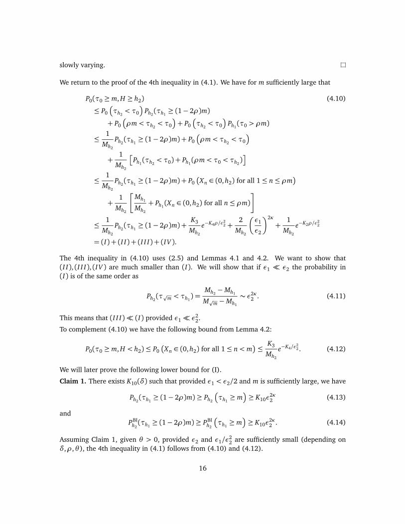
slowly varying.

We return to the proof of the 4th inequality in (4.1). We have for m sufficiently large that

P0(τ0 ≥ m, H ≥ h2) (4.10)

≤ P0

�

τh2< τ0

�

Ph2(τh1

≥ (1− 2ρ)m)

+ P0

�

ρm< τh2< τ0

�

+ P0

�

τh2< τ0

�

Ph1(τ0 > ρm)

≤1

Mh2

Ph2(τh1

≥ (1− 2ρ)m) + P0

�

ρm< τh2< τ0

�

+1

Mh2

�

Ph1(τh2

< τ0) + Ph1(ρm< τ0 < τh2

)�

≤1

Mh2

Ph2(τh1

≥ (1− 2ρ)m) + P0�

Xn ∈ (0, h2) for all 1≤ n≤ ρm�

+1

Mh2

�

Mh1

Mh2

+ Ph1(Xn ∈ (0, h2) for all n≤ ρm)

�

≤1

Mh2

Ph2(τh1

≥ (1− 2ρ)m) +K3

Mh2

e−K4ρ/ε22 +

2

Mh2

�

ε1

ε2

�2κ

+1

Mh2

e−K2ρ/ε22

= (I) + (I I) + (I I I) + (IV ).

The 4th inequality in (4.10) uses (2.5) and Lemmas 4.1 and 4.2. We want to show that(I I), (I I I), (IV ) are much smaller than (I). We will show that if ε1 � ε2 the probability in(I) is of the same order as

Ph2(τpm < τh1

) =Mh2−Mh1

Mpm−Mh1

∼ ε2κ2 . (4.11)

This means that (I I I)� (I) provided ε1� ε22.

To complement (4.10) we have the following bound from Lemma 4.2:

P0(τ0 ≥ m, H < h2)≤ P0�

Xn ∈ (0, h2) for all 1≤ n< m�

≤K3

Mh2

e−K4/ε22 . (4.12)

We will later prove the following lower bound for (I).

Claim 1. There exists K10(δ) such that provided ε1 < ε2/2 and m is sufficiently large, we have

Ph2(τh1

≥ (1− 2ρ)m)≥ Ph2

�

τh1≥ m

�

≥ K10ε2κ2 (4.13)

andPBI

h2(τh1

≥ (1− 2ρ)m)≥ PBIh2

�

τh1≥ m

�

≥ K10ε2κ2 . (4.14)

Assuming Claim 1, given θ > 0, provided ε2 and ε1/ε22 are sufficiently small (depending on

δ,ρ,θ), the 4th inequality in (4.1) follows from (4.10) and (4.12).

16

Our next task is to use the coupling of {Xn} to {X BIn }, from Section 3, to prove the 2nd and 5th

inequaltites in (4.1). Here h1± should be viewed as substitutes for h1 which allow an error ofηp

m in the coupling construction. Fix m/2 ≤ l ≤ m. We begin with the 5th inequality. Fromthe coupling construction we have

Ph2

�

τh1≥ l�

≤ PBIh2(τBI

h1−≥ l�

+ P∗h2(N(τBI

h1−)≥ η

pm,τBI

h1−< l ∧τh1

). (4.15)

We need to bound the last probability. Consider first δ 6= 0. Let A(x) = supy≥x a(y), soA(x) = o(1/x), and let d0 = h2

1−A(h1−)/|δ|. Suppose that for some time i and some evenintegers d0 ≤ d ≤ η

pm, the gap |X i − X BI

i | ≤ d and X BIi ≥ h1−. Provided h1− is large, by (3.1)

the misstep probability for the next step is then at most

A(h1−) +|δ|dh2

1−≤

2|δ|dh2

1−.

Let Gd0, Gd0+2, . . . , G2η

pm−2 be independent geometric random variables, with Gd having pa-

rameter 2|δ|d/h21−, and S = Gd0

+ Gd0+2 + · · · + G2ηp

m−2. The gap |X i − X BIi | can change

(always by 2) only at times of missteps. Therefore if we start from the time (if any) before τBIh1−

when the gap first reaches d0, the time until the next misstep (if any) before τBIh1−

is stochas-

tically larger than Gd0, and then the time until the misstep after that (if any) before τBI

h1−is

stochastically larger than Gd0+2, and so on. It follows that

P∗h2(N(τBI

h1−)≥ η

pm,τBI

h1−< l ∧τh1

)≤ P(S ≤ l)≤ P(S ≤ m). (4.16)

Note that for h1− large (depending on η/ε1),

E(S)m=

∑

d0≤d<2ηp

m,d−d0 even

h21−

2|δ|dm≥

h21−

4|δ|mlogηp

m

d0≥

ε21

32|δ|log

|δ|h1−A(h1−)

,

which grows to infinity as m → ∞; thus E(S) � m. In fact by standard computations usingexponential moments, we obtain that for some K11(η,δ,ε1) we have

P(S ≤ m)≤ e−K11p

m (4.17)

for all sufficiently large m, and hence by Claim 1,

P(S ≤ m)≤θ

2Ph2(τh1

≥ l). (4.18)

In the case δ = 0, {X BIn } is a symmetric simple RW so there are no discrepancies, only alarms,

which have probability at most A(h1)when the original RW is above height h1. Hence in place of(4.16) we have the left side of (4.16) bounded above by the probability that a Binomial(l, A(h1))exceeds η

pm, and this probability is also bounded by e−K11

pm, and then the same argument

applies. Now (4.13), (4.15), (4.16) and (4.18) show that provided m is large, the 5th inequalityin (4.1) holds.

17

Turning to the 2nd inequality in (4.1), the analog of (4.16) is still valid, so from the couplingconstruction, (4.17) and (4.14) (trivially modified to allow h1+ in place of h1), we have

Ph2(τh1

≥ m)≥ PBIh2(τBI

h1+≥ m)− P∗h2

(N(τh1)≥ η

pm,τh1

< m∧τBIh1+) (4.19)

≥ PBIh2(τh1+

≥ m)− e−K11p

m

≥ (1− θ)PBIh2(τh1+

≥ m),

proving the desired inequality.

The next step is to prove the first and last inequalities in (4.1), by relating the probabilitiesfor {X BI

n } to probabilities for the continuous-time Bessel process Yt . We need to establish thefollowing.

Claim 2. Given 0< ε1 < ε2, 0< ρ < 1/3 and θ > 0, for sufficiently large m,

PBIh2

�

τh1−≥ (1− 2ρ)m

�

≤ (1+ θ)PBeh2

�

τh1−≥ (1− 3ρ)m

�

, (4.20)

andPBI

h2(τh1+

≥ m)≥ (1− θ)PBeh2

�

τh1+≥ (1+ρ)m

�

. (4.21)

Suppose Claim 2 is proved. For the Bessel process we have the obvious inequality

PBeh2

�

τh1−≥ (1− 3ρ)m

�

≤ PBeh2

�

τ0 ≥ (1− 3ρ)m�

, (4.22)

whilePBe

h2

�

τh1+≥ (1+ρ)m

�

≥ PBeh2

�

τ0 ≥ (1+ 2ρ)m�

− PBeh1+

�

τ0 ≥ ρm�

. (4.23)

It follows from (15) in [23] that for δ >−1 and ε > 0,

PBeεp

t(τ0 ≥ t) =

∫ ε2/2

0

1

Γ(κ)uκ−1e−u du∼ K12ε

2κ as ε→ 0, (4.24)

where K12 = (2κκΓ(κ))−1. (Strictly speaking this seems to be stated in [23] only for Besselprocesses with dimension in (0, 2), i.e. δ ∈ (−1, 1), but the same proof works for nonpositivedimension, i.e. δ ≥ 1. The key is the 3 lines after (57) in Appendix B of [23].) Applying this toeach probability on the right side of (4.23) we see that for ρ and then ε1/ε2 taken sufficientlysmall and then m large, we have

PBeh1+

�

τ0 ≥ ρm�

≤ θ PBeh2

�

τ0 ≥ (1+ 2ρ)m�

,

and therefore by (4.23),

PBeh2

�

τh1+≥ (1+ρ)m

�

≥ (1− θ)PBeh2

�

τ0 ≥ (1+ 2ρ)m�

. (4.25)

Combining (4.21) and (4.25) we obtain the first inequality in (4.1), while the last inequality in(4.1) is a consequence of (4.20) and (4.22). This completes the proof of (4.1). Since ρ,θ canbe taken arbitrarily small, (4.1) together with (2.6) and (4.24) proves (2.7).

18

Proof of Claim 2. Let T0 = 0 and let T1, T2, . . . be the stopping times when the Bessel processreaches an integer different from the last integer it has visited, so that X BI

n = YTn. Denote the

hitting times of h1− in the two processes by τBIh1−

and τBeh1−

and letσi =min{t : Yt ∈ {i−1, i+1}}.Given k and x1, x2, . . . , xk, with x i ≥ h1−, let

A= {τBIh1−= k} ∩ {X BI

0 = h2, X BI1 = x1, . . . , X BI

k = xk}.

Conditionally on A, the random variables Ti−Ti−1, i ≤ k, are independent, with the distributionof Ti − Ti−1 being

PBex i−1

�

σx i−1∈ · | Yσxi−1

= x i�

.

The mean of this distribution is

EBeh2(Ti − Ti−1 | A) =

EBex i−1

�

σx i−1δ{Yσxi−1

=x i}�

PBex i−1(Yσxi−1

= x i). (4.26)

We need estimates for the quantities

EBex (σxδ{Yσx=x−1}), EBe

x (σx) and PBex (Yσx

= x − 1).

Let

s(x) =

(

x1+δ if δ 6=−1,

log x if δ =−1

be the scale function for the Bessel process and let L f given by

(L f )(x) =1

2f ′′(x)−

δ

2xf ′(x)

be its infinitesmal generator. For fixed x and z ∈ [x − 1, x + 1] the functions f = fx , g =gx , h± = h±x given by

f (z) = PBez (Yσx

= x − 1), g(z) = EBez (σx),

h±(z)s(x + 1)− s(x − 1)

= EBez (σxδ{Yσx=x±1})

satisfyL f ≡ 0, f (x − 1) = 1, f (x + 1) = 0;

L g ≡−1, g(x − 1) = g(x + 1) = 0;

(L h+)(z) = s(x − 1)− s(z), h+(x − 1) = h+(x + 1) = 0;

(L h−)(z) = s(z)− s(x + 1), h−(x − 1) = h−(x + 1) = 0.

These can be solved explicitly, yielding that for δ >−1,

f (z) =s(x + 1)− s(z)

s(x + 1)− s(x − 1),

19

g(z) =

− 11−δz2+ 4x

1−δ1

(x+1)1+δ−(x−1)1+δ z1+δ + Ax if δ 6= 1,

−z2 log z+ (x+1)2 log(x+1)−(x−1)2 log(x−1)4x

z2+ A′x if δ = 1,

h+(z) =

(

(x−1)1+δ

1−δ z2− 13+δz3+δ + Bxz1+δ + Dx if δ 6= 1,

(x − 1)2z2 log z− 14z4+ B′xz2+ D′x if δ = 1,

h−(z) =

(

− (x+1)1+δ

1−δ z2+ 13+δz3+δ + B′′x z1+δ + D′′x if δ 6= 1,

−(x + 1)2z2 log z+ 14z4+ B′′′x z2+ D′′′x if δ = 1.

Note the formulas here for δ = 1 are determined by the formulas for δ 6= 1, by continuity in δ.Here Bx is given by

(1−δ)Bx =−4x(x − 1)1+δ

(x + 1)1+δ − (x − 1)1−δ+

1−δ1+δ

(x − 1)2ψ1

�

2

x − 1

�

with

ψ1(u) =1+δ3+δ

(1+ u)3+δ − 1

(1+ u)1+δ − 1= 1+ u+

2+δ6

u2+O(u3) as u→ 0,

B′x is given by

B′x =1

2(x2+ 1)−

(x − 1)2(x + 1)2

4xlog�

1+2

x − 1

�

− (x − 1)2 log(x − 1),

and B′′x and B′′x are given by

(1−δ)B′′x =4x(x + 1)1+δ

(x + 1)1+δ − (x − 1)1−δ−

1−δ1+δ

(x − 1)2ψ1

�

2

x − 1

�

and

B′′′x =−1

2(x2+ 1) +

(x − 1)2(x + 1)2

4xlog�

1+2

x − 1

�

+ (x + 1)2 log(x + 1).

Finally, Ax , A′x and Dx , D′x and D′′x , D′′′x are determined by g(x − 1) = 0, h+(x − 1) = 0 andh−(x + 1) = 0, respectively, but we do not need these values because we can use for exampleg(x) = g(x)− g(x−1), and Ax or A′x cancels in the latter expression. From these computationswe readily obtain

f (x)→1

2, g(x)→ 1,

h±(x)s(x + 1)− s(x − 1)

→1

2as x →∞, (4.27)

and then also

EBex (σx | Yσx

= x − 1)→ 1, EBex (σx | Yσx

= x + 1)→ 1 as x →∞.

20

Therefore, uniformly in those A with all x i ≥ h1−, as m→∞ we have

EBeh2(Ti − Ti−1 | A)→ 1. (4.28)

It is easily seen by comparison to “Brownian motion plus small constant” that PBez (σx > 1) is

bounded away from 1 uniformly in (large) x and in z ∈ [x − 1, x + 1]. Hence by the Markovproperty PBe

x

�

σx > t) decays exponentially in t, uniformly in large x . By (4.27), this meansthere exist K13, K14 such that

PBex

�

σx > t | Yσx= x ± 1

�

≤max�

1

f (x),

1

1− f (x)

�

PBex

�

σx > t)≤ K13e−K14 t ,

for all t ≥ 0 and all (large) x . Therefore for m sufficiently large, for all A and t,

PBeh2(Ti − Ti−1 > t | A)≤ K13e−K14 t . (4.29)

By standard methods, it follows from (4.28) and (4.29) that for some K15(ρ), K16(ρ) not de-pending on A,

PBeh2

��

�

�τBeh1−−τBI

h1−

�

�

�> ρτBIh1−

�

� A�

= PBeh2

��

�Tk − k�

�> ρk�

� A�

≤ K15e−K16k. (4.30)

Therefore the same bound holds unconditionally, so

PBIh2

�

τBIh1−≥ (1− 2ρ)m

�

(4.31)

≤ PBeh2

�

τBeh1−≥ (1− 3ρ)m

�

+ PBeh2

�

τBIh1−≥ (1− 2ρ)m,

�

�

�τBeh1−−τBI

h1−

�

�

�> ρτBIh1−

�

≤ PBeh2

�

τBeh1−≥ (1− 3ρ)m

�

+ K15e−(1−2ρ)K16m

≤ (1+ θ)PBeh2

�

τBeh1−≥ (1− 3ρ)m

�

,

where the last inequality follows from (4.23) and (4.24), for large m. Thus (4.20) is proved.We have similarly from (4.30) (with τh1−

trivially replaced by τh1+) that

PBeh2

�

τBeh1+≥ (1+ρ)m

�

(4.32)

≤ PBeh2

�

τBIh1+≥ m

�

+ PBeh2

�

τBeh1+≥ (1+ρ)m,

�

�

�τBeh1+−τBI

h1+

�

�

�> ρτBIh1+

�

≤ PBIh2

�

τBIh1+≥ m

�

+ K15e−K16m

≤1

1− θPBI

h2

�

τBIh1+≥ m

�

,

so (4.21), and thus Claim 2, are also proved.

Proof of Claim 1. From (4.21), (4.25) and then(4.24), we have

PBIh2(τh1+

≥ m)≥ (1− θ)PBeh2

�

τh1+≥ (1+ρ)m

�

≥ (1− 2θ)PBeh2

�

τ0 ≥ (1+ 2ρ)m�

≥ K17ε2κ2 ,

21

and it is straightforward to replace τh1+here by τh1

, proving the second inequality in (4.14).The first inequality there is trivial.

The first inequality in (4.13) is also trivial, so we prove the second one. Using (4.14) and slightvariants of (4.16) and (4.17) we get that for large m,

Ph2(τh1

≥ m)≥ P∗h2

�

τBIh1+≥ m, N(m)≤ η

pm�

= P∗h2

�

τBIh1+≥ m

�

− P∗h2

�

τh1+≥ m, N(m)> η

pm�

≥ K10ε2κ2 − e−K2

pm

≥1

2K10ε

2κ2 ,

completing the proof of Claim 1.

This also completes the proof of (2.7), as noted after Claim 2.

5 Proof of (2.8) and (2.9)

For even numbers 0< m< n, let

fm = P0(τ0 = m), Am,n =2

n−m+ 2

n∑

j=m

f j .

Am,n is the average of the even-index f j ’s with j ∈ [m, n]. We use (2.10) and the followingconvexity property of { fm}.

Lemma 5.1. For all even numbers 0< k < m,

fm ≤fm+k + fm−k

2(5.1)

andfm ≤ Am−k,m+k. (5.2)

Proof. Let x= {x0, . . . , xm} be the trajectory of an excursion of length m starting at time 0, andx′ = {x ′k, . . . , x ′m+k} the trajectory of an excursion of length m starting at time k. (Necessarily,then, x0 = xm = x ′k = x ′m+k = 0 and all other x j and x ′j are positive.) Since k is even,there must be an s ∈ (k, m) with xs = x ′s; let T = T (x,x′) denote the least such s and Dt ={(x,x′) : T (x,x′) = t}. For x,x′ ∈ Dt , by switching the two trajectories after time t, we obtainan excursion y = y(x,x′) = {x0, . . . , x t , x ′t+1, . . . , x ′m+k} of length m+ k and an excursion y′ =y′(x,x′) = {x ′k, . . . , x ′t , x t+1, . . . , xm} of length m− k. The map (x,x′) 7→ (y,y′) is one to one andsatisfies

P0(x)P(x′ | Xk = 0) = P0(y)P(y

′ | Xk = 0).

22

It follows that

f 2m =

∑

t:k<t<m

∑

(x,x′)∈Dt

P0(x)P(x′ | Xk = 0)

=∑

t:k<t<m

∑

(x,x′)∈Dt

P0(y(x,x′))P(y′(x,x′) | Xk = 0)

≤

∑

y

P0(y)

!

∑

y′P(y′ | Xk = 0)

= fm+k fm−k

≤�

fm+k + fm−k

2

�2

.

Equation (5.2) is an immediate consequence of (5.1).

Let θ > 0. Provided η is sufficiently small (depending on θ), we have from (2.10), (2.11) andLemma 5.1 that for n large and even and k = 2bηn/2c,

P0(τ0 = n) = fn (5.3)

≤ An−k,n+k

=1

k+ 1P0�

(1−η)n≤ τ0 ≤ (1+η)n�

≤ (1+ θ)22−κκ

K0Γ(κ)n−(κ+1)L(

pn).

In the reverse direction, suppose fn < (1−θ)An−k,n−2 for some 0< k < n/2, with k, n even. ByLemma 5.1 we have

k/2∑

j=1

fn−2 j ≤k

4fn+

1

2

k/2∑

j=1

fn−4 j (5.4)

≤1− θ

2

k/2∑

j=1

fn−2 j +1

4

k/2∑

j=1

fn−4 j +1

4

k/2∑

j=1

fn−4 j+2+ fn−4 j−2

2

=1− θ

2

k/2∑

j=1

fn−2 j +1

4

k/2∑

j=1

fn−4 j +1

8

k/2∑

j=1

fn−4 j+2+1

8

(k+2)/2∑

j=2

fn−4 j+2

=1− θ

2

k/2∑

j=1

fn−2 j +1

4

k∑

m=2

fn−2m+1

8fn−2+

1

8fn−2k−2,

and therefore

1+ θ2

k/2∑

j=1

fn−2 j ≤1

4

k∑

j=1

fn−2 j +1

8fn−2k−2, (5.5)

23

which in the case k = 2bηn/2c gives

(1+ θ)P0�

(1−η)n≤ τ0 ≤ n− 2�

(5.6)

≤1

2P0�

(1− 2η)n≤ τ0 ≤ n− 2�

+1

4P0

�

τ0 = n− 4�ηn

2

�

− 2�

.

For small η and large n, this contradicts (2.7), showing that we cannot have fn < (1 −θ)An−k,n−2. Therefore for large n, using (2.7) we have

P0(τ0 = n) = fn (5.7)

≥ (1− θ)An−k,n−2

=2(1− θ)

kP0�

(1−η)n≤ τ0 ≤ n− 2�

≥ (1− 2θ)22−κκ

K0Γ(κ)n−(κ+1)L(

pn).

This and (5.3) prove (2.8).

We now prove (2.9). Let P denote the distribution of the Bessel-like RW dual to P, that is, thewalk with transition probabilities px = qx , qx = px for x ≥ 1. In [14] it is proved that for neven,

P(τ0 > n) = P(Xn = 0). (5.8)

For δ = −1, the dual walk has drift parameter δ = 1, so (2.9) follows by applying (2.8) and(2.20) to the dual walk.

6 Proof of Theorem 2.2

We want to use (2.13) so we need to approximate

f (k)n = Pk(τ0 = n) and Pk(Xn = 0).

We sometimes omit the superscript (k)when it is equal to 0. We start with the following relativeof Lemma 5.1.

Lemma 6.1. Let 0≤ p ≤ q ≤ r ≤ s ≤∞ and 0≤ k < l. Then for l − k even,

Pl(τ0 ∈ [p, q])Pk(τ0 ∈ [r, s])≤ Pl(τ0 ∈ [r, s])Pk(τ0 ∈ [p, q]), (6.1)

and for l − k odd,

Pl(τ0 ∈ [p, q])Pk(τ0 ∈ [r, s])≤ Pl(τ0 ∈ [r + 1, s+ 1])Pk(τ0 ∈ [p− 1, q− 1]). (6.2)

Proof. Suppose first that l − k is even. Consider a lattice path x starting at (0, k) in space-timewhich first hits the horizontal axis at a time in [r, s], and a lattice path x′ starting at (0, l) whichfirst hits the axis at a time in [p, q]. Since l − k is even, there must be a t ∈ (0, q] with x t = x ′t .

24

Switching the two trajectories after the first such t and proceeding as in Lemma 5.1 we obtain(6.1).

For l − k odd we repeat this argument but with the path x shifted one unit to the right, that is,started from (1, k).

Here are some special cases of interest for Lemma 6.1, particularly when comparing pointversus interval probabilities for τ0.

Corollary 6.2. (i) For all 0≤ k < l ≤ n and j > 0 with n− l and n+ j− k even,

f (k)n+ j

f (k)n

≤f (l)n+ j

f (l)n

if l − k is even, (6.3)

andf (k)n+ j

f (k)n−1

≤f (l)n+ j+1

f (l)n

if l − k is odd. (6.4)

(ii) For all 0≤ l ≤ m,Pl(τ0 = m)≤ Ml P0(τ0 = m) if l is even, (6.5)

andPl(τ0 = m)≤ Ml P0(τ0 = m− 1) if l is odd. (6.6)

(iii) For all l > 0 and 0≤ p < q < m,

Pl(τ0 = m)≥ Ml P0(τ0 = m)P0(τ0−τl ∈ [p, q])

P0(τ0 ∈ [p, q])if l is even, (6.7)

and

Pl(τ0 = m)≥ Ml P0(τ0 = m− 1)P0(τ0−τl ∈ [p, q])

P0(τ0 ∈ [p− 1, q− 1])if l is odd. (6.8)

By Corollary 6.2, to show that Pl(τ0 = m) can be well approximated by Ml P0(τ0 = m) (orMl P0(τ0 = m− 1), depending on parity), it is sufficient to find, given m, values p < q ≤ m forwhich the fraction in (6.7) or (6.8) is almost 1. We will see that this can be done for m� l2.

Proof of Corollary 6.2. (i) Take p = q = n and r = s = n+ j in Lemma 6.1 to get f (l)n f (k)n+ j ≤

f (l)n+ j f (k)n in the case of even l − k, and similarly for odd l − k.

(ii) Consider even l. We may assume m is also even, for otherwise the left side of (6.5) is 0.Applying Lemma 6.1 with k = 0, p = q = r = m and s =∞ we get

Pl(τ0 = m)≤Pl(τ0 ≥ m)P0(τ0 ≥ m)

P0(τ0 = m), (6.9)

while by (4.2),

1

MlPl(τ0 ≥ m)≤ P0(τ0 ≥ m). (6.10)

25

Together these prove (6.5). For odd l we may assume m is odd, and in place of (6.9) we get

Pl(τ0 = m)≤Pl(τ0 ≥ m+ 1)

P0(τ0 ≥ m)P0(τ0 = m− 1), (6.11)

and the rest of the proof is essentially unchanged, since Pl(τ0 ≥ m+ 1)≤ Pl(τ0 ≥ m).

(iii) Consider even l. We may assume m is even, for otherwise the right side of (6.7) is 0.Applying Lemma 6.1 with k = 0, [r, s] = {m} we obtain

Pl(τ0 = m)≥Pl(τ0 ∈ [p, q])P0(τ0 ∈ [p, q])

P0(τ0 = m), (6.12)

while by (2.3),

1

MlPl(τ0 ∈ [p, q]) = P0(τl < τ0)Pl(τ0 ∈ [p, q]) = P0(τ0−τl ∈ [p, q]), (6.13)

and together these prove (6.7). For odd l we may again assume m is odd and take [r, s] ={m− 1}, so that in place of (6.12), using (6.13) we get

Pl(τ0 = m)≥Pl(τ0 ∈ [p, q])

P0(τ0 ∈ [p− 1, q− 1])P0(τ0 = m− 1) (6.14)

= MlP0(τ0−τl ∈ [p, q])

P0(τ0 ∈ [p− 1, q− 1])P0(τ0 = m− 1).

Note that if we take k = 0 and j � n in (6.3), we see from (2.8) that the left side of (6.3) isclose to 1, so the right side cannot be much less than 1 for any l > 0.

For the Bessel process we have by (4.24) that for 0< a < b, recalling κ= (1+δ)/2,

PBek (τ0 ∈ [a, b]) =

∫ k2/2a

k2/2b

1

Γ(κ)uκ−1e−u du. (6.15)

As a step toward approximating Pk(Xn = 0)we have the following “interval” version of Theorem2.2, for midrange starting heights (k of order

pm); for these we apparently cannot get sharp

results from Corollary 6.2(ii) and (iii).

Proposition 6.3. Let θ > 0,χ > 0, 0 < ∆min < ∆max and 0 < a < b. Provided χ is sufficientlysmall (depending on θ), ∆max is sufficiently small (depending on θ ,χ),

b− a

b∈ [∆min,∆max], (6.16)

the starting height k is midrange, that is,

paχ ≤ k ≤

p

a/χ, (6.17)

26

and a is sufficiently large (depending on θ ,χ,∆min,∆max), we have

(1− θ)PBek (τ0 ∈ [a, b])≤ Pk(τ0 ∈ [a, b])≤ (1+ θ)PBe

k (τ0 ∈ [a, b]) (6.18)

and

1− θΓ(κ)

b− a

b

�

k2

2a

�κ

e−k2/2a ≤ Pk(τ0 ∈ [a, b]) (6.19)

≤1+ θΓ(κ)

b− a

b

�

k2

2a

�κ

e−k2/2a.

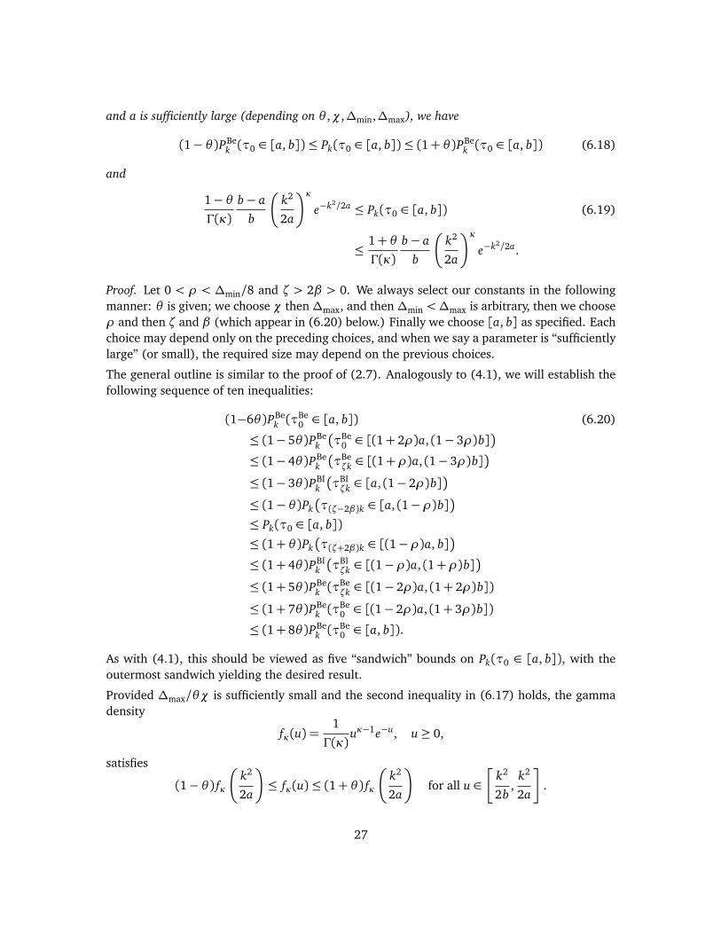
Proof. Let 0 < ρ < ∆min/8 and ζ > 2β > 0. We always select our constants in the followingmanner: θ is given; we choose χ then∆max, and then∆min <∆max is arbitrary, then we chooseρ and then ζ and β (which appear in (6.20) below.) Finally we choose [a, b] as specified. Eachchoice may depend only on the preceding choices, and when we say a parameter is “sufficientlylarge” (or small), the required size may depend on the previous choices.

The general outline is similar to the proof of (2.7). Analogously to (4.1), we will establish thefollowing sequence of ten inequalities:

(1−6θ)PBek (τ

Be0 ∈ [a, b]) (6.20)

≤ (1− 5θ)PBek

�

τBe0 ∈ [(1+ 2ρ)a, (1− 3ρ)b]

�

≤ (1− 4θ)PBek

�

τBeζk ∈ [(1+ρ)a, (1− 3ρ)b]

�

≤ (1− 3θ)PBIk

�

τBIζk ∈ [a, (1− 2ρ)b]

�

≤ (1− θ)Pk�

τ(ζ−2β)k ∈ [a, (1−ρ)b]�

≤ Pk(τ0 ∈ [a, b])

≤ (1+ θ)Pk�

τ(ζ+2β)k ∈ [(1−ρ)a, b]�

≤ (1+ 4θ)PBIk

�

τBIζk ∈ [(1−ρ)a, (1+ρ)b]

�

≤ (1+ 5θ)PBek (τ

Beζk ∈ [(1− 2ρ)a, (1+ 2ρ)b])

≤ (1+ 7θ)PBek (τ

Be0 ∈ [(1− 2ρ)a, (1+ 3ρ)b])

≤ (1+ 8θ)PBek (τ

Be0 ∈ [a, b]).

As with (4.1), this should be viewed as five “sandwich” bounds on Pk(τ0 ∈ [a, b]), with theoutermost sandwich yielding the desired result.

Provided ∆max/θχ is sufficiently small and the second inequality in (6.17) holds, the gammadensity

fκ(u) =1

Γ(κ)uκ−1e−u, u≥ 0,

satisfies

(1− θ) fκ

�

k2

2a

�

≤ fκ(u)≤ (1+ θ) fκ

�

k2

2a

�

for all u ∈�

k2

2b,

k2

2a

�

.

27

Then by (6.15),

PBek (τ0 ∈ [a, b])≥

1− θΓ(κ)

b− a

b

�

k2

2a

�κ

e−k2/2a (6.21)

and, using also the second inequality in (6.17),

PBek (τ0 ∈ [a, b])≤

1+ θΓ(κ)

b− a

b

�

k2

2a

�κ

e−k2/2a. (6.22)

Therefore (6.19) follows from (6.18). The inequalities (6.21) and (6.22), with minor modifi-cations made to θ , a and b, also prove the first and last inequalities in (6.20), provided ρ issuficiently small (depending on θ ,∆min,χ.)

Turning to the 2nd and 9th inequalities in (6.20), provided ζ2/ρχ is sufficiently small (depend-ing on θ), using (6.15) we have

PBek (τ0 ∈ [(1− 2ρ)a, (1+ 3ρ)b])≥ PBe

k

�

τζk ∈ [(1− 2ρ)a, (1+ 2ρ)b]�

PBeζk

�

τ0 ≤ ρb�

(6.23)

= PBek

�

τζk ∈ [(1− 2ρ)a, (1+ 2ρ)b]�

∫ ∞

ζ2k2/2ρb

1

Γ(κ)uκ−1e−u du

≥ (1− θ)PBek

�

τζk ∈ [(1− 2ρ)a, (1+ 2ρ)b]�

.

This proves the 9th inequality in (6.20). In the other direction,

PBek (τ0 ∈ [(1+ 2ρ)a, (1− 3ρ)b])≤ PBe

k

�

τζk ∈ [(1+ρ)a, (1− 3ρ)b]�

+ PBeζk

�

τ0 > ρa�

.(6.24)

From (6.16), (6.17) and (6.21),

PBek (τ0 ∈ [(1+ 2ρ)a, (1− 3ρ)b])≥

(1− θ)∆min

Γ(κ)

�

k2

2a

�κ

e−1/2χ , (6.25)

and hence by (4.24), provided ζ2/ρ is sufficiently small (depending on θ ,∆min,χ),

PBeζk

�

τ0 > ρa�

=

∫ ζ2k2/2ρa

0

1

Γ(κ)uκ−1e−u du (6.26)

≤1

κΓ(κ)

�

ζ2k2

2ρa

�κ

≤ θ PBek (τ0 ∈ [(1+ 2ρ)a, (1− 3ρ)b]).

With (6.24) this shows that

PBek (τ0 ∈ [(1+ 2ρ)a, (1− 3ρ)b])≤

1

1− θPBe

k

�

τζk ∈ [(1+ρ)a, (1− 3ρ)b]�

, (6.27)

which proves the 2nd inequality in (6.20).

28

Next we consider the 3rd and 8th inequalities in (6.20), in which Bessel-process probabilitiesare compared to similar probabilities for the imbedded RW. First, for the 8th inequality, analo-gously to (4.31) we have for some Ki = Ki(ρ) that

PBIk

�

τBIζk ∈ [(1−ρ)a, (1+ρ)b]

�

(6.28)

≤ PBek

�

τBeζk ∈ [(1− 2ρ)a, (1+ 2ρ)b]

�

+ PBek

�

τBIζk ∈ [(1−ρ)a, (1+ρ)b], |τBI

ζk −τBeζk|> ρa

�

≤ PBek

�

τBeζk ∈ [(1− 2ρ)a, (1+ 2ρ)b]

�

+ K18e−K19a.

By (6.17), (6.27) and (6.25), there exist K20 = K20(ρ,∆min,χ) and K21 = K21(ρ,∆min,χ,θ)such that for a ≥ K21,

PBek

�

τBeζk ∈ [(1− 2ρ)a, (1+ 2ρ)b]

�

≥ K20a−κ ≥1

θe−K19a, (6.29)

which with (6.28) and (6.23) shows that

PBIk

�

τBIζk ∈ [(1−ρ)a, (1+ρ)b]

�

≤ (1+ θ)PBek

�

τBeζk ∈ [(1− 2ρ)a, (1+ 2ρ)b]

�

, (6.30)

so the 8th inequality in (6.20) is proved. For the 3rd inequality, similarly to (6.28) and (6.30)we get

PBek

�

τBeζk ∈ [(1+ρ)a, (1− 3ρ)b]

�

≤ PBIk

�

τBIζk ∈ [a, (1− 2ρ)b]

�

+ e−K19a, (6.31)

which together with a slight modification of (6.29) gives

(1− θ)PBek

�

τBeζk ∈ [(1+ρ)a, (1− 3ρ)b]

�

≤ PBIk

�

τBIζk ∈ [a, (1− 2ρ)b]

�

, (6.32)

yielding the desired result.

Now we consider the 4th through 7th inequalities in (6.20), comparing probabilities for theimbedded RW to similar probabilities for the original RW, and comparing the hitting times of(ζ− 2β)k and 0; for this we use the coupling of {Xn} and {X BI

n }. First, for the 4th inequality,observe that for walks starting at k, if τBI

ζk ∈ [a, (1−2ρ)b] and the number of missteps by time

τBIζk is less than βk, then at time τBI

ζk, the stopping time τ(ζ−2β)k for the RW {Xn} has not yetoccurred and this RW is located in ((ζ− 2β)k, (ζ+ 2β)k). Therefore

PBIk

�

τBIζk ∈ [a, (1− 2ρ)b]

�

(6.33)

≤ P∗k�

τ(ζ−2β)k < τBIζk ∧ (1− 2ρ)b, N(τ(ζ−2β)k)≥ βk

�

+ P∗k�

τBIζk ∈ [a, (1− 2ρ)b],τ(ζ−2β)k > τ

BIζk, XτBI

ζk∈ ((ζ− 2β)k, (ζ+ 2β)k)

�

.

LetD = {τBI

ζk ∈ [a, (1− 2ρ)b],τ(ζ−2β)k > τBIζk, XτBI

ζk∈ ((ζ− 2β)k, (ζ+ 2β)k)}

denote the last event in (6.33). When D occurs, the RW {X BIn } reaches height ζk at some

time l, and when it does, the RW {Xn} is at some height j close to ζk, so {Xn} has a high

29

probability to reach height (ζ − 2β)k within an additional time ρb. More precisely, for j ∈((ζ−2β)k, (ζ+2β)k) and l ∈ [a, (1−2ρ)b], provided ζ2/ρχ is sufficiently small (dependingon θ), using (2.6), (2.7), (4.2) and our assumption a ≥ χk2 we have

P∗k�

τ(ζ−2β)k ∈ [a, (1−ρ)b] | D ∩ {τBIζk = l, X l = j}

�

(6.34)

= Pj�

τ(ζ−2β)k ≤ (1−ρ)b− l�

≥ Pj(τ(ζ−2β)k ≤ ρb�

≥ 1−M j P0(τ0 ≥ ρb)

≥ 1− θ .

Since l, j are arbitrary, the same bound holds if we just condition on D. From this and (6.33)we get

PBIk

�

τBIζk ∈ [a, (1− 2ρ)b]

�

(6.35)

≤ P∗k�

τ(ζ−2β)k < τBIζk ∧ (1− 2ρ)b, N(τ(ζ−2β)k)≥ βk

�

+1

1− θPk�

τ(ζ−2β)k ∈ [a, (1−ρ)b]�

.

Reasoning similarly to (4.17) using (6.17), and then using (6.21) and (6.32), we get that forsome K22(ζ,β) and K23(ζ,β ,θ ,∆min,χ), for a ≥ K23,

P∗k�

τ(ζ−2β)k < τBIζk ∧ (1− 2ρ)b, N(τ(ζ−2β)k)≥ βk

�

(6.36)

≤ e−K22p

a

≤ θ PBIk

�

τBIζk ∈ [a, (1− 2ρ)b]

�

.

With (6.35) this shows that

(1− θ)2PBIk

�

τBIζk ∈ [a, (1− 2ρ)b]

�

≤ Pk�

τ(ζ−2β)k ∈ [a, (1−ρ)b]�

, (6.37)

which yields the 4th inequality in (6.20).

For the 5th inequality in (6.20), from (2.6), (2.7), (4.2) and (6.17), provided ζ2/ρχ is suffi-ciently small (depending on θ), we have

P(ζ−2β)k�

τ0 > ρb�

≤ M(ζ−2β)kP0(τ0 ≥ ρb)≤ θ .

Hence

(1− θ)Pk�

τ(ζ−2β)k ∈ [a, (1−ρ)b]�

(6.38)

≤ Pk�

τ(ζ−2β)k ∈ [a, (1−ρ)b]�

P(ζ−2β)k�

τ0 ≤ ρb�

≤ Pk�

τ0 ∈ [a, b]�

,

which proves the 5th inequality.

30

Next, to prove the 7th inequality in (6.20), we can repeat (6.33)—(6.37) with {Xn} and {X BIn }

interchanged, and with ζk, (ζ−2β)k replaced by (ζ+2β)k,ζk, respectively, to obtain first thefollowing analog of (6.35) and (6.36):

Pk�

τ(ζ+2β)k ∈ [(1−ρ)a, b]�

(6.39)

≤ P∗k�

τBIζk < τ(ζ+2β)k ∧ b, N(τBI

ζk)≥ βk�

+1

1− θPk�

(τBIζk ∈ [(1−ρ)a, (1+ρ)b]

�

≤ θ Pk�

τ(ζ+2β)k ∈ [(1−ρ)a, b]�

+1

1− θPk�

(τBIζk ∈ [(1−ρ)a, (1+ρ)b]

�

,

and from this the analog of (6.37):

Pk�

τ(ζ+2β)k ∈ [(1−ρ)a, b]�

≤ (1+ 3θ)PBIk

�

τBIζk ∈ [(1−ρ)a, (1+ρ)b]

�

, (6.40)

so the 7th inequality is proved. Here for the second inequality in (6.39), analogously to (6.36),we require a lower bound for Pk

�

τ(ζ+2β)k ∈ [(1− ρ)a, b]�

, and this follows from (6.21) andthe inequality

Pk�

τ(ζ−2β)k ∈ [a, (1−ρ)b]�

≥1− 6θ

1− θPBe

k (τ0 ∈ [a, b])

which is contained in the first four inequalities of (6.20), with trivial modification to replaceζ− 2β with ζ+ 2β and [a, (1−ρ)b] with [(1−ρ)a, b].

For the 6th inequality, we have

Pk�

τ0 ∈ [a, b]�

≤ Pk�

τ(ζ+2β)k ∈ [(1−ρ)a, b]�

(6.41)

+ Pk�

τ(ζ+2β)k < (1−ρ)a,τ0 ∈ [a, b]�

.

Let us show that the last probability in (6.41) is much smaller than the first one. The Markovproperty at τ(ζ+2β)k, together with (2.6), (2.7), (4.2) and (6.17), yields that for some K24,provided a is sufficiently large,

Pk�

τ(ζ+2β)k < (1−ρ)a,τ0 ∈ [a, b]�

≤ P(ζ+2β)k�

τ0 ≥ ρa�

(6.42)

≤ M(ζ+2β)kP0(τ0 ≥ ρa)

≤ K24

�

ζ2k2

ρa

�κ

.

From (6.17), (6.21) and the first half of (6.20) we have that for some K25,

Pk�

τ0 ∈ [a, b]�

≥ (1− 6θ)PBek (τ0 ∈ [a, b])≥ K25∆mine−1/2χ

�

k2

a

�κ

.

From this and (6.42) we obtain that provided ζ2/ρ is sufficiently small (depending on∆min,θ ,χ), the ratio of the last to the first probability in (6.41) is at most θ , which with(6.41) shows that

(1− θ)Pk�

τ0 ∈ [a, b]�

≤ Pk�

τ(ζ+2β)k ∈ [(1−ρ)a, b]�

,

proving the 6th inequality in (6.20), which completes the full proof of (6.20). Statement (6.18)is then immediate, and then, as we have noted, (6.19) follows.

31

Let us now prove Theorem 2.2 for low starting heights—suppose that

1≤ k <pχm.

Let a ∈ [m/2, m). We will use Corollary 6.2(ii) and (iii), with [p, q] = [a/2, a], together with(2.8). By (2.8), provided ρ is sufficiently small (depending on θ) and then a is sufficientlylarge, we have

P0

�

τ0−τk ∈�a

2, a��

) (6.43)

≥ P0

�

τk ≤ ρa,τ0 ∈��

1

2+ρ�

a, a��

= P0

�

τ0 ∈��

1

2+ρ�

a, a��

�

1− P0

�

τk > ρa

�

�

�

�

τ0 ∈��

1

2+ρ�

a, a�

��

≥ (1− θ)P0

�

τ0 ∈�a

2, a��

�

1− P0

�

τk > ρa

�

�

�

�

τ0 ∈��

1

2+ρ�

a, a�

��

.

We need an upper bound for the conditional probability on the right side of (6.43). For someK26, K27 we have from (2.6), (2.7), (6.17) and Lemma 4.2 that provided χ is sufficiently small(depending on θ ,ρ),

P0

�

τk > ρa

�

�

�

�

τ0 ∈��

1

2+ρ�

a, a�

�

(6.44)

≤P0(τk ∧τ0 > ρa)

P0

�

τ0 ∈��

12+ρ�

a, a��

≤ K26e−K4ρa/k2

Mka−κL(p

a)

≤ K27L(k)

L(p

a)

� a

k2

�κ

e−K4ρa/k2

≤ θ .

Now (6.43), (6.44), (2.7) and (2.8) show that

P0

�

τ0−τk ∈�a

2, a��

)≥ (1− 2θ)P0

�

τ0 ∈�a

2, a��

(6.45)

≥ (1− 3θ)P0

�

τ0 ∈�a

2− 1, a− 1

��

which with Corollary 6.2(ii), (iii) shows that

(1− 3θ)MkP0(τ0 = m)≤ Pk(τ0 = m)≤ MkP0(τ0 = m), m even, (6.46)

(1− 3θ)MkP0(τ0 = m− 1)≤ Pk(τ0 = m)≤ MkP0(τ0 = m− 1), m odd. (6.47)

This and (2.8) prove (2.14).

32

Next we prove Theorem 2.2 for midrange starting heights–suppose

pmχ ≤ k ≤

r

m

χ.

Let θ > 0 and let 0 < ∆min < ∆max be as in Proposition 6.3. For the first inequality in (2.15)we use Corollary 6.2(i) and Proposition 6.3. From Corollary 6.2(i) and Theorem 2.1, for mlarge with m− k even, and 0 ≤ j < ∆minm with m− j even, provided ∆min is small enough(depending on θ), we have

f (k)m ≥f (0)m

f (0)m− j

f (k)m− j ≥ (1− θ) f(k)m− j if k is even, (6.48)

f (k)m ≥f (0)m−1

f (0)m− j−2

f (k)m− j−1 ≥ (1− θ) f(k)m− j−1 if k is odd, (6.49)

so that, averaging over j and applying Proposition 6.3, provided∆min is small enough (depend-ing on χ,θ),

Pk(τ0 = m)≥ (1− 2θ)2

∆minmPk((1−∆min)m< τ0 < m) (6.50)

≥ (1− 3θ)2

Γ(k)m

�

k2

2m

�κ

e−k2/2m.

For the second inequality in (2.15) the proof is similar: in place of (6.48) and (6.49) we havethat for m+ j even,

f (k)m ≤f (0)m

f (0)m+ j

f (k)m+ j ≤ (1+ θ) f(k)m+ j if k is even, (6.51)

f (k)m ≤f (0)m−1

f (0)m+ j

f (k)m+ j+1 ≤ (1+ θ) f(k)m+ j+1 if k is odd. (6.52)

and then as with (6.50),

Pk(τ0 = m)≤ (1+ θ)2

∆minmPk�

τ0 ∈ [m, (1+∆min)m]�

≤ (1+ 3θ)2

Γ(κ)m

�

k2

2m

�κ

e−k2/2m, (6.53)

completing the proof of (2.15).

Last, we prove Theorem 2.2 for high starting heights. We may assume k ≤ m. From the firstinequalities in (6.51) and (6.52) and from Theorem 2.1, averaging over j ∈ [0, m/8] we obtain

33

that for m large and 0< h< k/3 we have

Pk(τ0 = m)≤�

9

8

�κ 32

mPk

�

τ0 ∈�

m,9

8m��

≤�

9

8

�κ 32

mPk

�

τh ≤9

8m�

. (6.54)

To bound the last probability we couple our Bessel-like RW to a symmetric simple RW. Recallthat N(t) denotes the number of alarms by time t, and let

N ∗ =

�

�

�

�

�

i ≤9

8m : X i ≥ h, X sym

i ≥ h, and an alarm occurs at time i��

�

�

�

.

Analogously to (4.15) we have

Pk

�

τh ≤9

8m�

= P∗k

�

τsym3h > τh,τh ≤

9

8m�

+ P∗k

�

τsym3h ≤ τh ≤

9

8m�

≤ P∗k�

N ∗ > h�

+ Psymk

�

τsym3h ≤

9

8m�

. (6.55)

We now take h = k/8; we assume for convenience that h is an integer. If m0 (and hence k) islarge enough, then supx≥k/8 |px −

12| ≤ 2(1+ |δ|)/k. Then N ∗ is stochastically smaller than a

Binomial(9m/8,2(1+ |δ|)/k) random variable. We apply Bennett’s Inequality (see Hoeffding[26]), which states that for a Binomial(n, p) random variable Y and λ > np,

P(Y ≥ λ)≤ e−λψ(np(1−p)/λ),

where ψ is the decreasing function

ψ(x) = (1+ x) log�

1+1

x

�

− 1.

For x ≤ 1/4 we have ψ(x) ≥ 1 and hence ψ(x) ≥ 12(1+ x) log

�

1+ 1x

�

≥ 12

log 1x. Therefore

for λ≥ 4np,P(Y ≥ λ)≤ e−(λ/2) log(λ/np),

and in particular, provided χ is sufficiently small we have

P∗k

�

N ∗ >k

8

�

≤ e−(k/16) log(k2/18(1+|δ|)m) ≤ e−k/4 ≤ e−k2/4m. (6.56)

Also, again provided χ is small, by Hoeffding’s inequality [26],

Psymk

�

τsymk/4 ≤

9

8m�

≤ 2Psym0

�

X sym9m/8 >

3

4k�

≤ e−k2/4m,

which with (6.54), (6.55) and (6.56) yields

Pk(τ0 = m)≤�

9

8

�κ 64

me−k2/4m ≤

1

me−k2/8m, (6.57)

completing the proof of (2.16).

34

7 Proof of Theorems 2.3 and 2.4

Theorem 2.4 is a straightforward consequence of Theorem 2.3, (2.13) and (2.5), so we proveTheorem 2.3. We use (2.21), applying Theorem 2.2 and (2.18)—(2.20) to approximate theproducts on the right side.

We consider first part (i), for low starting heights, i.e. 1≤ k <pχn. By (2.7), (2.8) and (2.21)

and Theorem 2.2, given θ > 0, taking ρ and then χ sufficiently small, for n large, we have thefollowing sandwich bound for Pk(Xn = 0):

(1− 2θ)P0(X n = 0) (7.1)

≤ (1− θ) min(1−ρ)n≤ j≤n

P0(X j = 0)

≤ Pk(τ0 ≤ ρn) min(1−ρ)n≤ j≤n

P0(X j = 0)

≤ Pk(Xn = 0)

≤ max(1−ρ)n≤ j≤n

P0(X j = 0) +∑

0≤ j<(1−ρ)n

Pk(τ0 = n− j)P0(X j = 0)

≤ (1+ θ)P0(X n = 0) + max0≤i<(1−ρ)n

Pk(τ0 = n− i)∑

0≤ j<(1−ρ)n

P0(X j = 0)

≤ (1+ θ)P0(X n = 0) + K28(ρn)−(κ+1)L(p

n)Mpχn

∑

0≤ j<(1−ρ)n

P0(X j = 0).

We need to show that the second term on the right side of (7.1) is small compared to the firstterm on the right side. From (2.18)—(2.20) we see that for some K29, in all three cases, thesum in that second term is bounded by K29nP0(X n = 0). Therefore, using (2.6) and (2.8), if χis sufficiently small (depending on θ ,ρ) then for large n, the second term is bounded above by

2K28K29χκ

ρκ+1 P0(X n = 0)≤ θ P0(X n = 0).

With (7.1) this gives

(1− 2θ)P0(X n = 0)≤ Pk(Xn = 0)≤ (1+ 2θ)P0(X n = 0), (7.2)

as desired.

Next we consider part (ii), for E0(τ0) <∞ and midrange starting heights,p

nχ ≤ k ≤p

n/χ.By (2.18) there exists n1 such that

2− θE0(τ0)

≤ P0(Xn = 0)≤2+ θE0(τ0)

for all even n≥ n1.

Let 0 < χ < χ. Then using (2.21) and Theorem 2.2 (with χ in place of χ), provided χ is

35

sufficiently small, and then n (and hence k) is sufficiently large,

Pk(Xn = 0)≥n−χk2∑

j=n1

Pk(τ0 = n− j)P0(X j = 0) (7.3)

≥2− θE0(τ0)

∑

m:χk2≤m≤n−n1,m−k even

Pk(τ0 = m)

≥2− 3θ

E0(τ0)

∑

m:χk2≤m≤n−n1,m−k even

2

Γ(κ)m

�

k2

2m

�κ

e−k2/2m

≥2− 4θ

E0(τ0)

∫ n−n1

χk2

1

Γ(κ)x

�

k2

2x

�κ

e−k2/2x d x

=2− 4θ

E0(τ0)

∫ 1/2χ

k2/2(n−n1)

1

Γ(κ)uκ−1e−u du

≥2− 5θ

E0(τ0)

∫ ∞

k2/2n

1

Γ(κ)uκ−1e−u du.

In the other direction, we have similarly

n−χk2∑

j=n1

Pk(τ0 = n− j)P0(X j = 0)≤2+ 5θ

E0(τ0)

∫ ∞

k2/2n

1

Γ(κ)uκ−1e−u du. (7.4)

Also similarly to (7.3), given α > 0 we have for sufficiently small χ that provided n is large,

Pk(χk2 ≤ τ0 ≤ k2/χ)≥ (1−α)∫ 1/2χ

χ/2

1

Γ(κ)uκ−1e−u du≥ 1− 2α, (7.5)

so in particular, for small χ,

Pk(τ0 < χk2)≤ θ∫ ∞

1/2χ

1

Γ(κ)uκ−1e−u du.

36

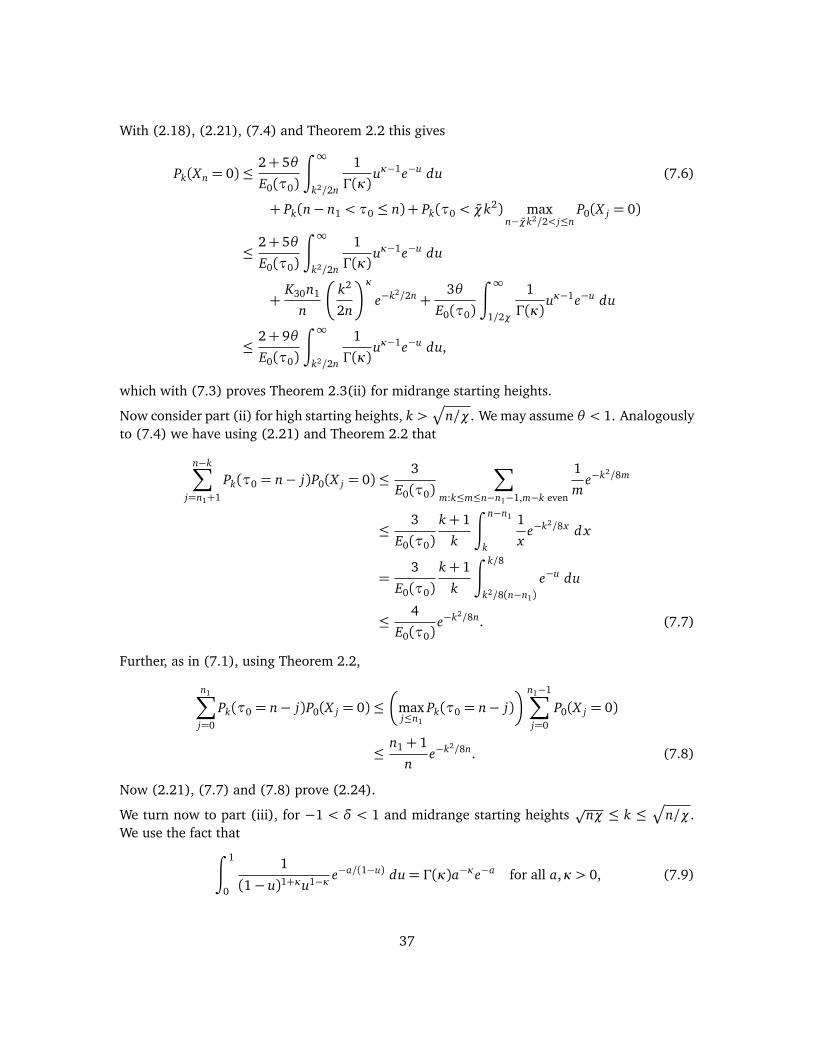
With (2.18), (2.21), (7.4) and Theorem 2.2 this gives

Pk(Xn = 0)≤2+ 5θ

E0(τ0)

∫ ∞

k2/2n

1

Γ(κ)uκ−1e−u du (7.6)

+ Pk(n− n1 < τ0 ≤ n) + Pk(τ0 < χk2) maxn−χk2/2< j≤n

P0(X j = 0)

≤2+ 5θ

E0(τ0)

∫ ∞

k2/2n

1

Γ(κ)uκ−1e−u du

+K30n1

n

�

k2

2n

�κ

e−k2/2n+3θ

E0(τ0)

∫ ∞

1/2χ

1

Γ(κ)uκ−1e−u du

≤2+ 9θ

E0(τ0)

∫ ∞

k2/2n

1

Γ(κ)uκ−1e−u du,

which with (7.3) proves Theorem 2.3(ii) for midrange starting heights.

Now consider part (ii) for high starting heights, k >p

n/χ. We may assume θ < 1. Analogouslyto (7.4) we have using (2.21) and Theorem 2.2 that

n−k∑

j=n1+1

Pk(τ0 = n− j)P0(X j = 0)≤3

E0(τ0)

∑

m:k≤m≤n−n1−1,m−k even

1

me−k2/8m

≤3

E0(τ0)k+ 1

k

∫ n−n1

k

1

xe−k2/8x d x

=3

E0(τ0)k+ 1

k

∫ k/8

k2/8(n−n1)e−u du

≤4

E0(τ0)e−k2/8n. (7.7)

Further, as in (7.1), using Theorem 2.2,

n1∑

j=0

Pk(τ0 = n− j)P0(X j = 0)≤�

maxj≤n1

Pk(τ0 = n− j)� n1−1∑

j=0

P0(X j = 0)

≤n1+ 1

ne−k2/8n. (7.8)

Now (2.21), (7.7) and (7.8) prove (2.24).

We turn now to part (iii), for −1 < δ < 1 and midrange starting heightsp

nχ ≤ k ≤p

n/χ.We use the fact that

∫ 1

0

1

(1− u)1+κu1−κ e−a/(1−u) du= Γ(κ)a−κe−a for all a,κ > 0, (7.9)

37

as can easily be seen via the change of variable v = (1−u)−1. By (2.19) there exists n2 = n2(θ)such that

(1− θ)2κK0

Γ(1−κ)n−(1−κ)L(

pn)−1 ≤ P0(Xn = 0)≤

(1+ θ)2κK0

Γ(1−κ)n−(1−κ)L(

pn)−1 (7.10)

for all even n≥ n2. Analogously to (7.3), provided χ/χ is sufficiently small, using (2.21), (7.9)and (7.10) we then obtain that for large n,

Pk(Xn = 0) (7.11)

≥n−χk2∑

j=n2

Pk(τ0 = n− j)P0(X j = 0)

≥(2− θ)2κK0

Γ(κ)Γ(1−κ)

∑

n2≤ j≤n−χk2

j even

1

n− j

�

k2

2(n− j)

�κ

e−k2/2(n− j) j−(1−κ)L(p

j)−1

≥(1− θ)2κK0

Γ(κ)Γ(1−κ)L(p

n)−1

∫ n−χk2

n2

1

n− x

�

k2

2(n− x)

�κ

e−k2/2(n−x) 1

x1−κ d x

=(1− θ)2κK0

Γ(κ)Γ(1−κ)n−(1−κ)L(

pn)−1

�

k2

2n

�κ ∫ 1−χk2/n

n2/n

1

(1− u)1+κu1−κ e−k2/2n(1−u) du

≥(1− 2θ)2κK0

Γ(1−κ)n−(1−κ)L(

pn)−1e−k2/2n.

In the other direction, analogously to (7.4), from a calculation similar to (7.11) we get

n−χk2∑

j=n2

Pk(τ0 = n− j)P0(X j = 0)≤(1+ 2θ)2κK0

Γ(1−κ)n−(1−κ)L(

pn)−1e−k2/2n. (7.12)

With (2.21), (2.19) and Theorem 2.2 this gives the analog of (7.6): provided χ is taken suffi-ciently small and then n sufficiently large,

Pk(Xn = 0) (7.13)

≤(1+ 2θ)2κK0

Γ(1−κ)n−(1−κ)L(

pn)−1e−k2/2n

+ n2 max0≤ j<n2

Pk(τ0 = n− j) + Pk(τ0 < χk2) maxn−χk2< j≤n

P0(X j = 0)

≤(1+ 2θ)2κK0

Γ(1−κ)n−(1−κ)L(

pn)−1e−k2/2n

+ K31(χ)n−1+ θ

(1+ 2θ)2κK0

Γ(1−κ)n−(1−κ)L(

pn)−1

≤(1+ 4θ)2κK0

Γ(1−κ)n−(1−κ)L(

pn)−1e−k2/2n.

38

Here the second inequality uses the fact that by (7.5), we can make Pk(τ0 < χk2) as small asdesired by taking χ small. Together (7.11) and (7.13) prove Theorem 2.3(iii) for midrangestarting heights.

We turn next to part (iii) for high starting heights, k >p

n/χ. There exists K32 such that for0< α≤ K2

32,∞∑

j=1

e−α j 1

j1−κL(p

j)≤

2

κα−κL

�

1pα

�−1

. (7.14)

Then analogously to (7.3) and (7.11), when k ≤ K32n, using (2.21), (7.10) and Theorem 2.2we have for large n,

n−k∑

j=n2

Pk(τ0 = n− j)P0(X j = 0)

≤21+κK0

Γ(1−κ)

n−k∑

j=n2

1

n− je−k2/8(n− j) 1

j1−κL(p

j)

≤22+κK0

Γ(1−κ)

�

2

ne−k2/8n

∑

n2≤ j≤n/2

e−k2 j/8n2 1

j1−κL(p

j)

+∑

n/2< j≤n−k

1

n− je−k2/8(n− j) 1

j1−κL(p

j)

�

≤22+κK0

Γ(1−κ)

�

4 · 4κ

κne−k2/8n

�n

k

�2κL�n

k

�−1+

2

ne−k2/4n

n∑

j=1

1

j1−κL(p

j)

�

≤22+κK0

Γ(1−κ)

�

4 · 4κ

κne−k2/8n

�n

k

�2κL�n

k

�−1+

4

κne−k2/4nnκL(

pn)−1

�

. (7.15)

Here in the third inequality we used the fact that (n− j)−1e−k2/8(n− j) is a decreasing functionof j, and the fact that L is slowly varying. Provided χ is sufficiently small, the second terminside the brackets on the right side of (7.15) is smaller than the first term; using this, (2.21)and Theorem 2.2 we obtain that for some K33(κ), provided χ is small enough,

Pk(Xn = 0)≤24+3κK0K32

κΓ(1−κ)ne−k2/8n

�n

k

�2κL�n

k

�−1+∑

0≤ j<n2

Pk(τ0 = n− j)

≤24+3κK0K32

κΓ(1−κ)ne−k2/8n

�n

k

�2κL�n

k

�−1+

2n2

ne−k2/8n

≤ K33e−k2/8nn−(1−κ)L(p

n)−1. (7.16)

Here n2 = n2(1). This proves (2.26) when k ≤ K32n. If K32n < k ≤ n, in place of (7.15) and

39

(7.16) we have using (2.16) that

Pk(Xn = 0) =n−k∑

j=0

Pk(τ0 = n− j)P0(X j = 0)

≤n−k∑

j=0

1

n− je−k2/8n

≤ K34e−k2/8n, (7.17)

from which (2.26) follows.

Next we consider part (iv), in which δ = 1, E0(τ0) =∞, in the case of midrange starting heightsp

nχ ≤ k ≤p

n/χ. In this case µ0 is slowly varying, and by (2.20) there exists n3 = n3(θ) suchthat

2− θµ0(n)

≤ P0(Xn = 0)≤2+ θµ0(n)

for all even n≥ n3. (7.18)

Then analogously to (7.3), using Theorem 2.2, (2.21) and (7.18), for large n,

Pk(Xn = 0)≥n−χk2∑

j=n3

Pk(τ0 = n− j)P0(X j = 0) (7.19)

≥4− 3θ

Γ(κ)

∑

χk2≤m≤n−n3n−m even

1

m

�

k2

2m

�κ

e−k2/2m 1

µ0(n−m)

≥2− 2θ

µ0(n)

∫ ∞

k2/2n

1

Γ(κ)uκ−1e−u du,

and similarly

n−χk2∑

j=n3

Pk(τ0 = n− j)P0(X j = 0)≤2+ 2θ

µ0(n)

∫ ∞

k2/2n

1

Γ(κ)uκ−1e−u du. (7.20)

Using (2.21), (7.18), (7.20) and Theorem 2.2, and taking χ sufficiently small, we obtain the

40

analog of (7.13):

Pk(Xn = 0) (7.21)

≤2+ 2θ

µ0(n)

∫ ∞

k2/2n

1

Γ(κ)uκ−1e−u du

+ n3 max0≤ j<n3

Pk(τ0 = n− j) + Pk(τ0 < χk2) maxn−χk2< j≤n

P0(X j = 0)

≤2+ 2θ

µ0(n)

∫ ∞

k2/2n

1

Γ(κ)uκ−1e−u du

+ K35(χ)n−1+

θ

µ0(n)

∫ ∞

1/2χ

1

Γ(κ)uκ−1e−u du

≤2+ 4θ

µ0(n)

∫ ∞

k2/2n

1

Γ(κ)uκ−1e−u du.

Together (7.19) and (7.21) prove Theorem 2.3(iv) for midrange starting heights.

Last we consider part (iv) for high starting heights, k >p

n/χ. We may assume θ < 1. Whenk ≤ K32n and k is sufficiently large, we have analogously to (7.15), using (7.14) and Theorem2.2,

n−k∑

j=n3

Pk(τ0 = n− j)P0(X j = 0)

≤n−k∑

j=n3

1

n− je−k2/8(n− j) 3

µ0( j)

≤6

ne−k2/8n

∑

n3≤ j≤n/2

e−k2 j/8n2 1

µ0( j)+

6

ne−k2/4n

∑

n/2< j≤n−k

1

µ0( j)

≤96

ne−k2/8n n2

k2µ0

�

n2

k2

�−1

+ e−k2/4n 6

µ0(n)

≤ e−k2/8n 7

µ0(n). (7.22)

In the last inequality we have bounded (n2/k2)µ0(n2/k2)−1 by n/96µ0(n), valid for χ suffi-ciently small because n2/k2 ≤ χ2n and µ0 is slowly varying. Then using (2.21) and (2.16),

Pk(Xn = 0)≤ e−k2/8n 7

µ0(n)+∑

1≤ j<n3

Pk(τ0 = n− j)

≤ e−k2/8n 7

µ0(n)+

n3

ne−k2/8n

≤ e−k2/8n 8

µ0(n). (7.23)

41

If instead K32n < k ≤ n, then (7.17) is valid. In fact, a look at (6.57) shows that, by reducingχ if necessary, we can replace 8 on the right side of (7.17) with any constant greater than 4.Therefore in place of (7.23) we have for large n that

Pk(Xn = 0)≤ K34e−k2/6n ≤1

µ0(n)e−k2/8n. (7.24)

Thus (2.28) holds in both cases.

8 Acknowledgements

The author thanks P. Baxendale, F. Dunlop, T. Huillet, J. Pitman and A. Wade for helpful discus-sions, and thanks a referee for multiple references and suggestions.

References

[1] Alexander, K. S. (2008). The effect of disorder on polymer depinning transitions. Com-mun. Math. Phys. 279 117–146. MR2377630 MR2377630

[2] Alexander, K.S. and Zygouras, N. (2009). Quenched and annealed critical points in poly-mer pinning models. Commun. Math. Phys. 291 659–689. MR2534789 MR2534789

[3] Aspandiiarov, S. and Iasnogorodski, R. (1997). Tails of passage-times and an applicationto stochastic processes with boundary reflection in wedges. Stoch. Proc. Appl. 66, 115–145. MR1431874 MR1431874

[4] Aspandiiarov, S. and Iasnogorodski, R. (1999). General criteria of integrability of func-tions of passage-times for nonnegative stochastic processes and their applications. Theor.Probab. Appl. 43, 343–369. MR1681072 MR1681072

[5] Aspandiiarov, S., Iasnogorodski, R. and Menshikov, M. (1996). Passage-time momentsfor nonnegative stochastic processes and an application to reflected random walks in aquadrant. Ann. Probab. 24, 932–960. MR1404537 MR1404537

[6] Brezis, H., Rosenkrantz, W. and Singer, B. (1971). An extension of Khintchine’s estimatefor large deviations to a class of Markov chains converging to a singular diffusion. Comm.Pure Appl. Math. 24, 705–726. MR0300347 MR0300347

[7] Carmona, P. and Hu, Y. (2002). On the partition function of a directed polymer in arandom environment. Probab. Theory. Rel. Fields, 124, 431-457. MR1939654 MR1939654

[8] Coolen-Schrijner, P. and van Doorn, E. A. (1998). Analysis of random walks using orthog-onal polynomials. J. Comp. Appl. Math. 99, 387–399. MR 1662710 MR1662710

[9] Comets, F. and Yoshida, N. (2007). Directed polymers in random environments are diffu-sive at weak disorder. Ann. Probab. 34, 1746-1770. MR2271480 MR2271480

42

[10] Csáki, E., Földes, A. and Révész, P. (2009). Transient nearest neighbor random walk andBessel process. J. Theoret. Probab. 22, 992–1009. MR2558662 MR2558662

[11] de Coninck, J., Dunlop, F. and Huillet, T. (2008). Random walk weakly attracted to a wall.J. Stat. Phys. 133, 271–280. MR 2448534 MR2448534

[12] de Coninck, J., Dunlop, F. and Huillet, T. (2009). Random walk versus random line. Phys.A 388, 4034–4040. MR 2552859 MR2552859

[13] Dette, H. (2001). First return probabilities of birth and death chains and associated or-thogonal polynomials. Proc. Amer. Math. Soc. 129, 1805–1815. MR1814114 MR1814114

[14] Dette, H., Fill, J. A., Pitman, J. and Studden, W. J. (1997). Wall and Siegmund dualityrelations for birth and death chains with reflecting barrier. J. Theor. Probab. 10, 349–374.MR1455149 MR1455149

[15] Doney, R.A. (1997). One-sided local large deviation and renewal theorems in the case ofinfinite mean. Probab. Theory Rel. Fields 107, 451–465. MR1440141 MR1440141

[16] Erickson, K. B. (1970). Strong renewal theorems with infinite mean. Trans. Amer. Math.Soc. 151, 263–291. MR0268976 MR0268976

[17] Fal’, A. M. (1981). Certain limit theorems for an elementary Markov random walk.Ukrainian Math. J. 33, 433–435. [Translated from Ukrain. Mat. Zh. 33 (1981), 564–566.]MR0627740 MR0627740

[18] Fal’, A. M. (1973). On the simplest Markov random walk. Soviet Math. Dokl. 14, 1071–1074. [Translated from Dokl. Akad. Nauk SSSR 211 (1973), 540–542.] MR0326845MR0326845

[19] Feller, W. (1968). An Introduction to Probability Theory and its Applications Vol. I, 3rd ed.Wiley, New York. MR0228020 MR0228020

[20] Giacomin, G. (2007). Random Polymer Models. Imperial College Press, London. MR2380992 MR2380992

[21] Giacomin, G., Lacoin, H. and Toninelli, F. (2009). Disorder relevance at marginality andcritical point shift. arXiv:0906.1942v1 [math-ph]

[22] Giacomin, G. and Toninelli, F. (2005). Smoothing effect of quenched disorder on polymerdepinning transitions. Commun. Math. Phys. 266 1–16. MR2231963 MR2231963

[23] Göing-Jaeschke, A. and Yor, M. (2003). A survey and some generalizations of Bessel pro-cesses. Bernoulli 9, 313–349. MR1997032 MR1997032

[24] Halpin-Healy, T. and Zhang, Y.-C. (1995). Kinetic roughening phenomena, stochasticgrowth, directed polymers and all that. Phys. Reports 254, 215–414.

43

[25] Hodges, J. L., Jr. and Rosenblatt, M. (1953). Recurrence-time moments in random walks.Pacific J. Math. 3, 127–136. MR0054190 MR0054190

[26] Hoeffding, W. (1963). Probability inequalities for sums of bounded random variables. J.Amer. Statist. Assoc. 58, 13–30. MR0144363 MR0144363

[27] Jain, N. C. and Pruitt, W.E. (1972). The range of random walk. In Proceedings of the SixthBerkeley Symposium on Mathematical Statistics and Probability (Univ. California, Berkeley,Calif., 1970/1971), Vol. III: Probability Theory, 31-50. Univ. California Press, Berkeley,Calif. MR0410936 MR0410936

[28] Karlin, S. and McGregor, J. L. (1957a). The differential equations of birth-and-deathprocesses, and the Stieltjes moment problem. Trans. Amer. Math. Soc. 85, 489–546.MR0091566 MR0091566

[29] Karlin, S. and McGregor, J. L. (1957b). The classification of birth and death processes.Trans. Amer. Math. Soc. 86, 366–400. MR0094854 MR0094854

[30] Karlin, S. and McGregor, J. (1959). Random walks. Ill. J. Math. 3, 66–81. MR0100927MR0100927

[31] Lacoin, H. (2010). New bounds for the free energy of directed polymers in dimension1+ 1 and 1+ 2. Commun. Math. Phys. 294 471–503. MR2579463 MR2579463

[32] Lamperti, J. (1962). A new class of probability limit theorems. J. Math. Mech. 11, 749–772. MR0148120 MR0148120

[33] Lamperti, J. (1963). Criteria for stochastic processes II: Passage-time moments. J. Math.Anal. Appl. 7, 127–145. MR0159361 MR0159361

[34] Menshikov, M. V. and Popov, S. Yu. (1995). Exact power estimates for countable Markovchains. Markov. Proc. Rel. Fields 1, 57–78. MR1403077 MR1403077

[35] Menshikov, M. V., Vachkovskaia, M. and Wade, A. R. (2008). Asymptotic behaviour ofrandomly reflecting billiards in unbounded tubular domains. J. Stat. Phys. 132, 1097–1133. MR2430776 MR2430776

[36] Revuz, D. and Yor, M. (1991). Continuous Martingales and Brownian Motion. Grundlehrender Mathematischen Wissenschaften [Fundamental Principles of Mathematical Sciences],293. Springer-Verlag, Berlin, New York. MR 1083357 MR1083357

[37] Rosenkrantz, W. A. (1966). A local limit theorem for a certain class of random walks. Ann.Math. Statist. 37, 855–859. MR0200988 MR0200988

44