11

EXECUTION PLANOPTIMIZATIONTECHNIQUESJulius StroffekDatabase Sustaining EngineerSun Microsystems, Inc.

Tomas KovarıkFaculty of Mathematics and Physics,Charles University, Prague

PostgreSQL Conference, 2007

OutlineMotivation

Definition of The Problem

Deterministic Algorithms for Searching the Space

Non-Deterministic Algorithms for Searching the Space

Demo

Algorithms Already Implemented for Query Optimization

Experimental Performance Comparison

Demo

Conclusions

Motivation

Motivation

Questions which come to mind looking at PostgreSQLoptimizer implementation:

I Why to use genetic algorithm?I Does this implementation behave well?I What about other ”Soft Computing” methods?I Are they worse, the same or better?I What is the optimizer’s bottle-neck?

Goals

I Focus on algorithms for searching the spaceI Present ideas how PostgreSQL optimizer might be

improvedI Receive feedbackI Discuss the ideas within the communityI Implement some of those ideas

Definition of The Problem

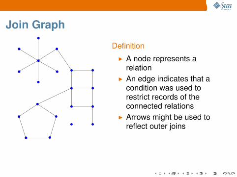
Join Graph

DefinitionI A node represents a

relationI An edge indicates that a

condition was used torestrict records of theconnected relations

I Arrows might be used toreflect outer joins

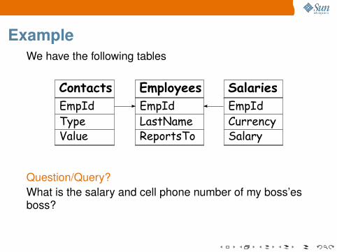
ExampleWe have the following tables

Question/Query?What is the salary and cell phone number of my boss’esboss?

Optimizer and Execution Plan

Lets have a query like thisselectbboss.EmpId, sal.Salary,sal.Currency, con.Value

fromEmployees as emp,Employees as boss,Employees as bboss,Salaries as sal,Contacts as con

whereemp.LastName=’MyName’and emp.ReportsTo = boss.EmpIdand boss.ReportsTo = bboss.EmpIdand bboss.EmpId = sal.EmpIdand con.EmpId = bboss.EmpIdand con.Type = ’CELL’

How to process the query?

I There are 5 relations tobe joined

I If we do not allow productjoins we have 10 options

I With product joinsallowed we have 60options

Join Graph for the Example Query

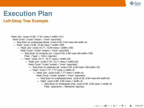
Execution PlanLeft-Deep Tree Example

Hash Join (cost=13.84..17.81 rows=1 width=151)Hash Cond: (”outer”.empid = ”inner”.reportsto)→ Seq Scan on employees bboss (cost=0.00..3.64 rows=64 width=4)→ Hash (cost=13.84..13.84 rows=1 width=159)→ Hash Join (cost=10.71..13.84 rows=1 width=159)

Hash Cond: (”outer”.empid = ”inner”.reportsto)→ Seq Scan on contacts con (cost=0.00..2.80 rows=64 width=136)

Filter: (”type” = ’CELL’::bpchar)→ Hash (cost=10.71..10.71 rows=1 width=23)→ Hash Join (cost=7.78..10.71 rows=1 width=23)

Hash Cond: (”outer”.empid = ”inner”.reportsto)→ Seq Scan on sallaries sal (cost=0.00..2.28 rows=128 width=19)→ Hash (cost=7.77..7.77 rows=1 width=4)→ Hash Join (cost=3.80..7.77 rows=1 width=4)

Hash Cond: (”outer”.empid = ”inner”.reportsto)→ Seq Scan on employees boss (cost=0.00..3.64 rows=64 width=8)→ Hash (cost=3.80..3.80 rows=1 width=4)→ Seq Scan on employees emp (cost=0.00..3.80 rows=1 width=4)

Filter: (lastname = ’MyName’::bpchar)

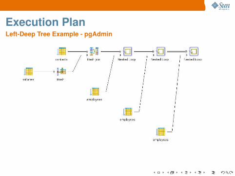
Execution PlanLeft-Deep Tree Example - pgAdmin

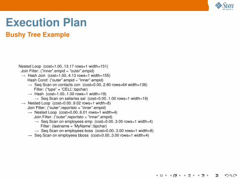
Execution PlanBushy Tree Example

Nested Loop (cost=1.00..13.17 rows=1 width=151)Join Filter: (”inner”.empid = ”outer”.empid)→ Hash Join (cost=1.00..4.13 rows=1 width=155)

Hash Cond: (”outer”.empid = ”inner”.empid)→ Seq Scan on contacts con (cost=0.00..2.80 rows=64 width=136)

Filter: (”type” = ’CELL’::bpchar)→ Hash (cost=1.00..1.00 rows=1 width=19)→ Seq Scan on sallaries sal (cost=0.00..1.00 rows=1 width=19)

→ Nested Loop (cost=0.00..9.02 rows=1 width=8)Join Filter: (”outer”.reportsto = ”inner”.empid)→ Nested Loop (cost=0.00..6.01 rows=1 width=4)

Join Filter: (”outer”.reportsto = ”inner”.empid)→ Seq Scan on employees emp (cost=0.00..3.00 rows=1 width=4)

Filter: (lastname = ’MyName’::bpchar)→ Seq Scan on employees boss (cost=0.00..3.00 rows=1 width=8)

→ Seq Scan on employees bboss (cost=0.00..3.00 rows=1 width=4)

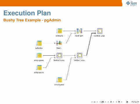
Execution PlanBushy Tree Example - pgAdmin

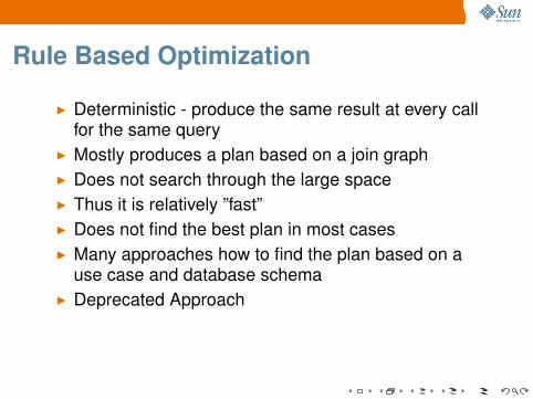
Rule Based Optimization

I Deterministic - produce the same result at every callfor the same query

I Mostly produces a plan based on a join graphI Does not search through the large spaceI Thus it is relatively ”fast”I Does not find the best plan in most casesI Many approaches how to find the plan based on a

use case and database schemaI Deprecated Approach

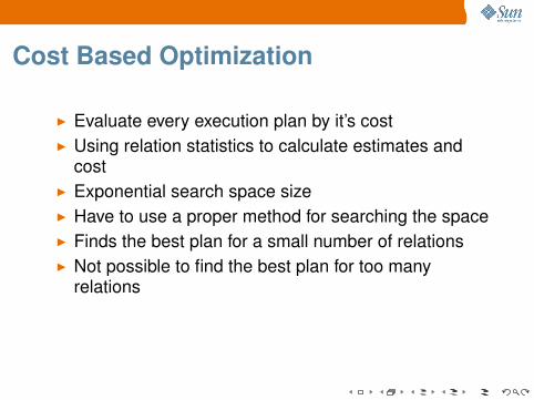
Cost Based Optimization

I Evaluate every execution plan by it’s costI Using relation statistics to calculate estimates and

costI Exponential search space sizeI Have to use a proper method for searching the spaceI Finds the best plan for a small number of relationsI Not possible to find the best plan for too many

relations

Deterministic Algorithms

Dynamic Programming

I Checks all possible orders of relationsI Applicable only for small number of relationsI Pioneered by IBM’s System R database projectI Iteratively creates and computes costs for every

combination of relations. Start with an access to anevery single relation. Later, compute the cost of joinsof every two relations, afterwards do the same formore relations.

Dynamic ProgrammingExample

Four relations to be joined – A, B, C and D.

Dijkstra’s algorithmDescription

A graph algorithm which finds the shortest path from asource node to any destination node in a weightedoriented graph

I A graph has to have a non-negative weight functionon edges

I The weight of the path is the sum of weights on edgeson the path

QuestionHow can we manage that the path will go through all thenodes/relations in a join graph?

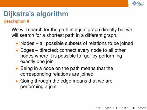
Dijkstra’s algorithmDescription II

We will search for the path in a join graph directly but wewill search for a shortest path in a different graph.

I Nodes – all possible subsets of relations to be joinedI Edges – directed; connect every node to all other

nodes where it is possible to “go” by performingexactly one join

I Being in a node on the path means that thecorresponding relations are joined

I Going through the edge means that we areperforming a join

Dijkstra’s algorithmGraph Example

We are joining four relations - A, B, C and D.

Dijkstra’s algorithmDescription III

For each node V we will maintainI The lowest cost c(V ) of already found path to achieve

the nodeI The state of the node – open/closed

We will also maintain a set of nodesM which will holdopen nodes

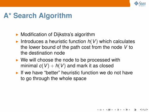
A* Search Algorithm

I Modification of Dijkstra’s algorithmI Introduces a heuristic function h(V ) which calculates

the lower bound of the path cost from the node V tothe destination node

I We will choose the node to be processed withminimal c(V ) + h(V ) and mark it as closed

I If we have “better” heuristic function we do not haveto go through the whole space

A* Search AlgorithmPossible Heuristic Functions

I The number of tuples in the current nodeI Reduces paths where too many tuples are prodcedI Applicable only in materialization nodes

I The number of tuples that need to be fetched from theremaining relations

I A “realistic” lower boundI Might be extended to get a lower bound of the cost of

remaining joins

I Any other approximation?

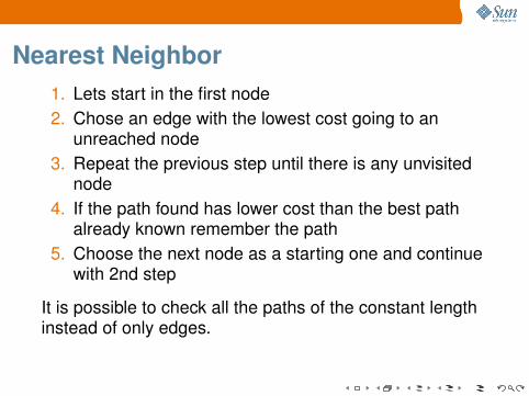
Nearest Neighbor1. Lets start in the first node2. Chose an edge with the lowest cost going to an

unreached node3. Repeat the previous step until there is any unvisited

node4. If the path found has lower cost than the best path

already known remember the path5. Choose the next node as a starting one and continue

with 2nd step

It is possible to check all the paths of the constant lengthinstead of only edges.

Nearest Neighbor for Bushy Trees

1. Build a set of nodes with an access to every relation2. Choose the cheapest join from all the combinations of

possible joins of any two relations from the set3. Add the result node to the set of relations to be joined4. Remove the originating relations from the set5. Go back to 2nd step if we still have more than one

relation

It is also possible to look forward for more joins at once.

Non-Deterministic Algorithms

Random Walk

Randomly goes through the search space

1. Set the MAX VALUE as a cost for the best knownpath

2. Choose a random path3. If the cost of the chosen path is better than the

currently best known remember the path as the best4. Go back to step 2

Very naive, not very usable in practise but can be used forcomparison with other algorithms

Simulated AnnealingIt is an analogy with physics – a cooling process ofa crystal.

A crystal has lots of energy and small random changesare happening in its structure. These small changes aremore stable if the crystal emits the energy afterwards.

An execution plan has a high cost at the begining. A smallrandom change is generated in every iteration of theprocess. Depending upon the cost change the probabilitywhether the change is preserved or discarded iscomputed. The change is kept with the computedprobability.

Hill-Climbing

1. Start with a random path2. Check all the neighbor paths and find the one with the

lowest cost3. If the cost of the best neighboring path is lower than

the actual one change the actual one to that neighbor4. Go back to 2nd step if we found a better path in the

previous step

DemoTravelling Salesman Problem

A travelling salesman has N cities which he needs to visit.He would like to find the shortest path going through allthe cities.

I Similar to the execution plan optimization problemI The evaluation function has different properties

I The evaluation of an edge between two cities does notdepend on the cities already visited

I Different behavior of heuristic algorithms

Implemented Algorithms

Implemented Algorithms

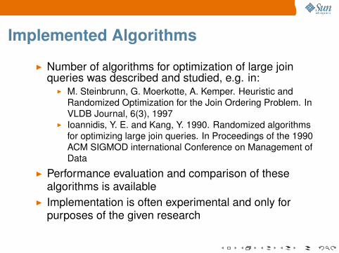
I Number of algorithms for optimization of large joinqueries was described and studied, e.g. in:

I M. Steinbrunn, G. Moerkotte, A. Kemper. Heuristic andRandomized Optimization for the Join Ordering Problem. InVLDB Journal, 6(3), 1997

I Ioannidis, Y. E. and Kang, Y. 1990. Randomized algorithmsfor optimizing large join queries. In Proceedings of the 1990ACM SIGMOD international Conference on Management ofData

I Performance evaluation and comparison of thesealgorithms is available

I Implementation is often experimental and only forpurposes of the given research

Studied algorithms

We will look at the following algorithms in more detail

I Genetic AlgorithmI Simulated AnnealingI Iterative ImprovementI Two Phase OptimizationI Toured Simulated Annealing

Genetic Algorithm

I Well known to the PostgreSQL community - GEQO -GEnetic Query Optimizer

I Fundamentally different approach designed tosimulate biological evolution

I Works always on a set of solutions called populationI Solutions are represented as character strings by

appropriate encoding.I In our case query processing trees

I Quality, or “fitness” of the solution is measured by anobjective function

I Evaluation cost of processing tree, has to be minimized

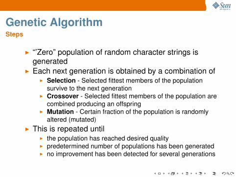
Genetic AlgorithmSteps

I “’Zero” population of random character strings isgenerated

I Each next generation is obtained by a combination ofI Selection - Selected fittest members of the population

survive to the next generationI Crossover - Selected fittest members of the population are

combined producing an offspringI Mutation - Certain fraction of the population is randomly

altered (mutated)I This is repeated until

I the population has reached desired qualityI predetermined number of populations has been generatedI no improvement has been detected for several generations

Simulated Annealing

I Doesn’t have to improve on every moveI Doesn’t get “trapped” in local minimum so easilyI Exact behavior determined by parameters:

I starting temperature (e.g. function of node cost)I temperature reduction (e.g. 90% of the old value)I stopping condition (e.g. no improvement in certain number

of temperature reductions)

I Performance of the algorithm is dependent on thevalues of these parameters

Simulated AnnealingDetermining neighbor states

I Join method choiceI Left-deep processing trees solution space

represented by an ordered list of relations to be joinedI Swap – exchange position of two relations in the listI 3Cycle – Cyclic rotation of three relations in the list

I Complete solution space including bushy treesI Join commutativity A ./ B→ B ./ AI Join associativity (A ./ B) ./ C↔ A ./ (B ./ C)I Left join exchange (A ./ B) ./ C↔ (A ./ C) ./ BI Right join exchange A ./ (B ./ C)↔ B ./ (A ./ C)

Iterative Improvement

I Strategy similar to Hill climbing algorithmI Overcomes the problem of reaching local minimumI Steps of the algorithm

I Select random starting pointI Choose random neighbor, if the cost is lower than the

current node, carry out the moveI Repeat step 2 until local minimum is reachedI Repeat all steps until stopping condition is metI Return the local minimum with the lowest cost

I Stopping condition can be processing fixed number ofstarting points or reaching the time limit

Two Phase Optimization

I Combination of SA and II, uses advantages of bothI Rapid local minimum discoveryI Search of the neighborhood even with uphill moves

I Steps of the algorithmI Predefined number of starting points selected randomlyI Local minima sought using Iterative improvementI Lowest of these minima is used as a starting point of

simulated annealing

I Initial temperature of the SA is lower, since only smallproximity of the minimum needs to be covered

Toured Simulated Annealing

I Simulated annealing algorithm is run several timeswith different starting points

I Starting points are generated using somedeterministic algorithm with reasonable heuristic

I The initial temperature is much lower than with thegeneric simulated annealing algorithm

I Benefits over plain simulated annealingI Covering different parts of the search spaceI Reduced running time

Experimental PerformanceComparision

Experimental Performance ComparisonWhat to consider

I Evaluation plan quality vs. running timeI Different join graph types

I ChainI StarI CycleI Grid

I Left-deep tree optimization vs. Bushy treeoptimization

I Algorithms involvedI Genetic algorithm (Bushy genetic algorithm)I Simulated annealing, Iterative improvement, Two phase

optimization

Experimental Performance ComparisonResults

I Bushy tree optimization yields better resultsespecially for chain and cycle join graphs.

I If solution quality is preferred, 2PO achieves betterresults (although slightly sacrificing the running time).

I Iterative improvement and Genetic algorithm aresuitable in case the running time is more important.

I Pure Simulated annealing requires higher runningtime without providing better solutions.

Demo

Conclusions

Conclusions

I We have presented an overview of algorithms usablefor query optimization

I Choosing the best algorithm is difficultI PostgreSQL has configuration parameters for GEQO

I ThresholdI Population sizeI Number of populationsI Effort based approach

I More configurable optimizer with different algorithmsI OLAP - would prefer better plan optimizationI OLTP - would prefer faster plan optimization

11

Julius StroffekJulius.Stroffek@Sun.COMjulo@stroffek.net

Tomas Kovarıktkovarik@gmail.com