executive master in finance risky debt professor andré farber solvay business school université...

Executive Master in FinanceRisky debt

Professor André Farber

Solvay Business School

Université Libre de Bruxelles

EMF 2006 Risky debt |2April 18, 2023

Recently in the Financial Times

• GM bond fall knocks wider markets

• GM’s debt downloaded to BBB- (just above junk status)

• Stock price: $29 (MarketCap $16.4b)

• Debt-per-share: $320 (Total debt $300b)

• Cumulative Default Probability 48% (CreditGrades calculation)


Credit risk

• Credit risk exist derives from the possibility for a borrower to default on its obligations to pay interest or to repay the principal amount.

• Two determinants of credit risk:

• Probability of default

• Loss given default / Recovery rate

• Consequence:

• Cost of borrowing > Risk-free rate

• Spread = Cost of borrowing – Risk-free rate

(usually expressed in basis points)

• Function of a rating

– Internal (for loans)

– External: rating agencies (for bonds)


Rating Agencies

• Moody’s (www.moodys.com)

• Standard and Poors (www.standardandpoors.com)

• Fitch/IBCA (www.fitchibca.com)

• Letter grades to reflect safety of bond issue

S&P AAA AA A BBB BB B CCC D

Moody’s Aaa Aa A Baa Ba B Caa C

Very High Quality

High Quality

Speculative Very Poor

Investment-grades Speculative-grades


Spread over Treasury for Industrial Bonds

Reuters Corporate Spreads for IndustrialJanuary 2004

http://bondchannel.bridge.com/publicspreads.cgi?Industrial

AAA AAA AAA AAA AAA AAAAAA

AA AA AA AA AA AAAA

A AA A A A A

BBBBBB

BBB BBB BBB BBBBBB

BB

BBBB

BB BB BB

BBB

B

BB

BB

B

0

100

200

300

400

500

600

0 5 10 15 20 25 30

Maturity

Sp

read


Determinants of Bonds Safety

• Key financial ratio used:– Coverage ratio: EBIT/(Interest + lease & sinking fund payments)

– Leverage ratio

– Liquidity ratios

– Profitability ratios

– Cash flow-to-debt ratio

• Rating Classes and Median Financial Ratios, 1998-2000

Rating Category

Coverage Ratio

Cash Flow to Debt %

Return on Capital %

LT Debt to Capital %

AAA 21.4 84.2 34.9 13.3

AA 10.1 25.2 21.7 28.2

A 6.1 15.0 19.4 33.9

BBB 3.7 8.5 13.6 42.5

BB 2.1 2.6 11.6 57.2

B 0.8 (3.2) 6.6 69.7

Source: Bodies, Kane, Marcus 2005 Table 14.3


Moody’s:Average cumulative default rates 1920-1999 %

1 2 3 4 5 10 15 20

Aaa 0.00 0.00 0.02 0.09 0.20 1.09 1.89 2.38

Aa 0.08 0.25 0.41 0.61 0.97 3.10 5.61 6.75

A 0.08 0.27 0.60 0.97 1.37 3.61 6.13 7.47

Baa 0.30 0.94 1.73 2.62 3.51 7.92 11.46 13.95

Inv. Grade 0.16 0.49 0.93 1.43 1.97 4.85 7.59 9.24

Ba 1.43 3.45 5.57 7.80 10.04 19.05 25.95 30.82

B 4.48 9.16 13.73 17.56 20.89 31.90 39.17 43.70

Spec. Grade 3.35 6.76 9.98 12.89 15.57 25.31 32.61 37.74

All Corp. 1.33 2.76 4.14 5.44 6.65 11.49 15.35 17.79


Modeling credit risk

• 2 approaches:

• Structural models (Black Scholes, Merton, Black & Cox, Leland..)

– Utilize option theory

– Diffusion process for the evolution of the firm value

– Better at explaining than forecasting

• Reduced form models (Jarrow, Lando & Turnbull, Duffie Singleton)

– Assume Poisson process for probability default

– Use observe credit spreads to calibrate the parameters

– Better for forecasting than explaining


Merton (1974)

• Limited liability: equity viewed as a call option on the company.

E Market value of equity

FFace value

of debt

VMarket value of comany

Bankruptcy

D Market value of debt

FFace value

of debt

VMarket value of comany

F

Loss given default


Using put-call parity

• Market value of firm:

V = E + D

• Put-call parity (European options)

Stock = Call + PV(Strike) – Put

• In our setting:

• V ↔Stock The company is the underlying asset

• E↔Call Equity is a call option on the company

• F↔Strike The strike price is the face value of the debt

• → D = PV(Strike) – Put

• D = Risk-free debt - Put


Merton Model: example using binomial option pricing

492.1 teu 670.1

ud

462.670.0492.1

67.05.11

du

drp f

Data:Market Value of Unlevered Firm: 100,000Risk-free rate per period: 5%Volatility: 40%

Company issues 1-year zero-couponFace value = 70,000Proceeds used to pay dividend or to buy back shares

f

du

r

fppff

1

)1(

V = 100,000E = 34,854D = 65,146

V = 67,032E = 0D = 67,032

V = 149,182E = 79,182D = 70,000

∆t = 1

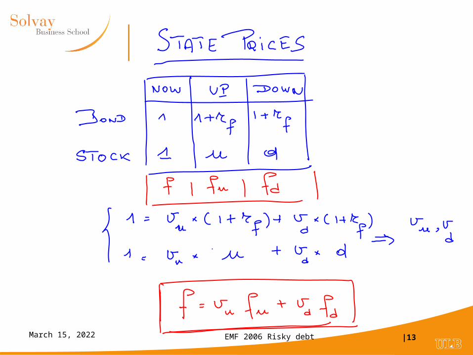
Binomial option pricing: reviewUp and down factors:

Risk neutral probability :

1-period valuation formula

05.1

032,67538.0000,70462.0 D

05.1

0538.0000,80462.0 E


Calculating the cost of borrowing

• Spread = Borrowing rate – Risk-free rate

• Borrowing rate = Yield to maturity on risky debt

• For a zero coupon (using annual compounding):

• In our example:

Ty

FD

)1(

y

1

000,70146,65

y = 7.45%

Spread = 7.45% - 5% = 2.45% (245 basis points)


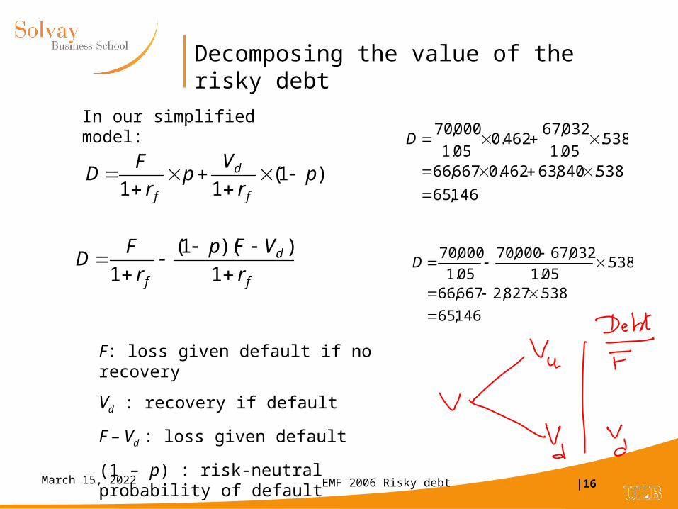
Decomposing the value of the risky debt

f

d

f r

VFp

r

FD

1

))(1(

1

)1(11

pr

Vp

r

FD

f

d

f

146,65

538.827,2667,66

538.05.1

032,67000,70

05.1

000,70

D

In our simplified model:

F: loss given default if no recovery

Vd : recovery if default

F – Vd : loss given default

(1 – p) : risk-neutral probability of default

146,65

538.840,63462.0667,66

538.05.1

032,67462.0

05.1

000,70

D


Weighted Average Cost of Capital

• (1) Start from WACC for unlevered company

– As V does not change, WACC is unchanged

– Assume that the CAPM holds

WACC = rA = rf + (rM - rf)βA

– Suppose: βA = 1 rM – rf = 6%

WACC = 5%+6%× 1 = 11%

• (2) Use WACC formula for levered company to find rE

V

Dr

V

Err DEA

000,100

146,65

000,100

854,34%11 DE rr

000,100

146,65

000,100

854,341 DE V

D

V

EDEA


Cost (beta) of equity

• Remember : C = Deltacall × S - B

– A call can is as portfolio of the underlying asset combined with borrowing B.

• The fraction invested in the underlying asset is X = (Deltacall × S) / C

• The beta of this portfolio is X βasset

• When analyzing a levered company:

– call option = equity

– underlying asset = value of company

– X = V/E = (1+D/E)

)1(E

DDelta

E

VDelta AAE

In example:βA = 1DeltaE = 0.96V/E = 2.87βE= 2.77rE = 5% + 6% × 2.77 = 21.59%

dSuS

ffDelta du

:Reminder


Cost (beta) of debt

• Remember : D = PV(FaceValue) – Put

• Put = Deltaput × V + B (!! Deltaput is negative: Deltaput=Deltacall – 1)

• So : D = PV(FaceValue) - Deltaput × V - B

• Fraction invested in underlying asset is X = - Deltaput × V/D

• βD = - βA Deltaput V/D

In example:βA = 1DeltaD = 0.04V/D = 1.54βD= 0.06rD = 5% + 6% × 0.09 = 5.33%

Putdudu

D DeltadSuS

PutPut

dSuS

PutFPutFDelta

)()(


Multiperiod binomial valuation

V

uV

u²V

u3V

u4V

dV

d²V

udV

u2dV

u3dV

u2d²V

ud3V

d4V

ud²V

d3V

p4

4p3(1 – p)

6p²(1 – p)²

4p (1 – p)3

(1 – p)4

Δt

Risk neutral proba

For European option, (1) At maturity, calculate

- firm values;- equity and debt values- risk neutral probabilities

(2) Calculate the expected values in a neutral world(3) Discount at the risk free rate


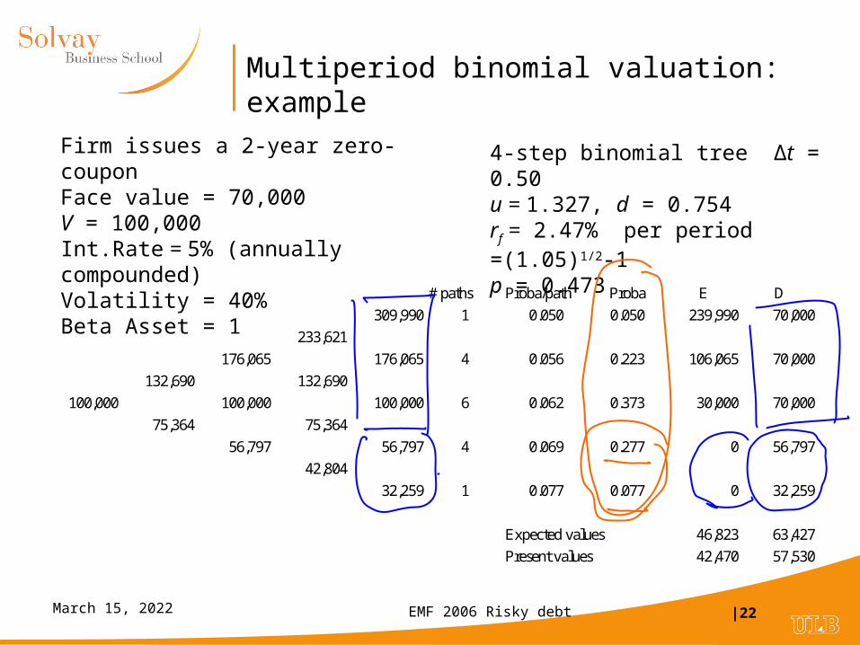
Multiperiod binomial valuation: example

Firm issues a 2-year zero-couponFace value = 70,000V = 100,000Int.Rate = 5% (annually compounded)Volatility = 40%Beta Asset = 1

4-step binomial tree Δt = 0.50u = 1.327, d = 0.754rf = 2.47% per period =(1.05)1/2-1p = 0.473

# paths Proba/path Proba E D

309,990 1 0.050 0.050 239,990 70,000

233,621

176,065 176,065 4 0.056 0.223 106,065 70,000

132,690 132,690

100,000 100,000 100,000 6 0.062 0.373 30,000 70,000

75,364 75,364

56,797 56,797 4 0.069 0.277 0 56,797

42,804

32,259 1 0.077 0.077 0 32,259

Expected values 46,823 63,427

Present values 42,470 57,530


Multiperiod valuation: details

Down Firm value0 100,000 132,690 176,065 233,621 309,9901 75,364 100,000 132,690 176,0652 56,797 75,364 100,0003 42,804 56,7974 32,259

Equity value42,470 69,427 109,399 165,308 239,990

20,280 36,828 64,377 106,0656,388 13,843 30,000

0 00

Delta0.86 0.95 1.00 1.00

0.70 0.88 1.000.43 0.69

0.00Beta

2.02 1.82 1.61 1.412.62 2.39 2.06

3.78 3.78#DIV/0!

Debt value57,530 63,262 66,667 68,313 70,000

55,084 63,172 68,313 70,00050,409 61,521 70,000

42,804 56,79732,259

Delta0.14 0.05 0.00 0.00

0.30 0.12 0.000.57 0.31

1.00Beta

0.25 0.10 0.00 0.000.40 0.19 0.00

0.65 0.371.00


Multiperiod binomial valuation: additional details

• From the previous calculation, we can decompose D into:

• Risk-free debt

• Risk-neutral probability of default

• Expected loss given default

• Expected value at maturity:

• Risk-free debt = 70,000

• Default probability = 0.354

• Expected loss given default = 18,552

• Risky debt = 70,000 – 0.354 × 18,552 = 63,427

• Present value:

• D = 63,427 / (1.05)² = 57,530


Toward Black Scholes formulas

Increase the number to time steps for a fixed maturity

The probability distribution of the firm value at maturity is lognormal

Time

Value

Today

Bankruptcy

Maturity


Black-Scholes: Review

• European call option: C = S N(d1) – PV(X) N(d2)

• Put-Call Parity: P = C – S + PV(X)

• European put option: P = + S [N(d1)-1] + PV(X)[1-N(d2)]

• P = - S N(-d1) +PV(X) N(-d2)

Delta of call option Risk-neutral probability of exercising the option = Proba(ST>X)

Delta of put option Risk-neutral probability of exercising the option = Proba(ST<X)

(Remember: 1-N(x) = N(-x))

TT

XPV

S

d

5.)

)(ln(

1 TT

XPV

S

d

5.)

)(ln(

2


Black-Scholes using Excel

23456789

10111213141516171819202122232425

A B C D EData Variable Comments and formulas

Stock price S 100.00Strike price Strike 70.00Maturity T 2Interest rate rf 4.88% with continuous compoundingVolatility Sigma 40.00%

Intermediate resultsPV(Strike price) PVStrike 63.49 D10. =Strike*EXP(-rf*T)ln(S/PV(Strike)) 45.43% D11. =LN(S/PVStrike)Sigma*t0.5 AdjSigma 56.57% D12. =Sigma*SQRT(T)Distance to exercice DTE 0.803 D13. =LN(S/PVStrike)/AdjSigmad1 1.0859 D14. =DTE+0.5*AdjSigmad2 0.5202 D15. =DTE-0.5*AdjSigma

CallCall 41.77 D18. =S*NORMSDIST(D14)-PVStrike*NORMSDIST(D15)Delta 0.86 D19. =NORMSDIST(D14)Proba in-the-money 0.30 D20. =1-NORMSDIST(D15)

PutPut 5.26 D23. =-S*NORMSDIST(-D14)+D10*NORMSDIST(-D15)Delta 0.14 D24. =NORMSDIST(-D14)Proba in-the-money 0.70 D25. =1-NORMSDIST(-D15)


Merton Model: example

DataMarket value unlevered firm €100,000Risk-free interest rate (an.comp): 5%Beta asset 1Market risk premium 6%Volatility unlevered 40%

Company issues 2-year zero-couponFace value = €70,000Proceed used to buy back shares

Using Black-Scholes formulaPrice of underling asset 100,000Exercise price 70,000Volatility 0.40Years to maturity 2Interest rate 5%

Value of call option 41,772Value of put option (using put-call parity) C+PV(ExPrice)-Sprice 5,264

Details of calculation:PV(ExPrice) = 70,000/(1.05)²= 63,492log[Price/PV(ExPrice)] = log(100,000/63,492) = 0.4543√t = 0.40 √ 2 = 0.5657

d1 = log[Price/PV(ExPrice)]/ √ + 0.5 √ t = 1.086

d2 = d1 - √ t = 1.086 - 0.5657 = 0.520

N(d1) = 0.861

N(d2) = 0.699

C = N(d1) Price - N(d2) PV(ExPrice)= 0.861 × 100,000 - 0.699 × 63,492= 41,772


Valuing the risky debt

• Market value of risky debt = Risk-free debt – Put Option

D = e-rT F – {– V[1 – N(d1)] + e-rTF [1 – N(d2)]}

• Rearrange:

D = e-rT F N(d2) + V [1 – N(d1)]

)](1[)(1

)(1 )( 2

2

12 dN

dN

dNVdNFeD rT

Value of risk-free

debt

Probability of no default

Probability of default

× ×Discounted

expected recovery

given default

+


Example (continued)

D = V – E = 100,000 – 41,772 = 58,228

D = e-rT F – Put = 63,492 – 5,264 = 58,228

228,583015.0031,466985.0492,63

)](1[)(1

)(1 )( 2

2

12

dNdN

dNVdNFeD rT

031,466985.01

8612.01000,100

)(1

)(1

2

1

dN

dNV


Expected amount of recovery

• We want to prove: E[VT|VT < F] = V erT[1 – N(d1)]/[1 – N(d2)]

• Recovery if default = VT

• Expected recovery given default = E[VT|VT < F] (mean of truncated lognormal distribution)

• The value of the put option:

• P = -V N(-d1) + e-rT F N(-d2)

• can be written as

• P = e-rT N(-d2)[- V erT N(-d1)/N(-d2) + F]

• But, given default: VT = F – Put

• So: E[VT|VT < F]=F - [- V erT N(-d1)/N(-d2) + F] = V erT N(-d1)/N(-d2)

Discount factor


Expected value of put given

F

F

Default

Put

Recovery

VT


Another presentation

Discount factor

Face Value


Expected loss given default

Loss if no recovery

Expected Amount of recovery given default

])(1

)(1[)](1[

2

12 dN

dNVeFdNFeD rTrT

]749,50000,70[3015.0000,1009070.0 D


Example using Black-Scholes

DataMarket value unlevered company € 100,000Debt = 2-year zero coupon Face value € 60,000

Risk-free interest rate 5%Volatility unlevered company 30%

Using Black-Scholes formula

Market value unlevered company € 100,000Market value of equity € 46,626Market value of debt € 53,374

Discount factor 0.9070N(d1) 0.9501N(d2) 0.8891

Using Black-Scholes formula

Value of risk-free debt € 60,000 x 0.9070 = 54,422

Probability of defaultN(-d2) = 1-N(d2) = 0.1109

Expected recovery given defaultV erT N(-d1)/N(-d2) = (100,000 / 0.9070) (0.05/0.11)= 49,585

Expected recovery rate | default= 49,585 / 60,000 = 82.64%


Calculating borrowing cost

Initial situation

Balance sheet (market value)Assets 100,000 Equity 100,000

Note: in this model, market value of company doesn’t change (Modigliani Miller 1958)

Final situation after: issue of zero-coupon & shares buy back

Balance sheet (market value)

Assets 100,000 Equity 41,772

Debt 58,228

Yield to maturity on debt y:

D = FaceValue/(1+y)²

58,228 = 60,000/(1+y)²

y = 9.64%

Spread = 364 basis points (bp)


Determinant of the spreads

0

200

400

600

800

1000

1200

1400

0 0.05 0.1 0.15 0.2 0.25 0.3 0.35 0.4 0.45 0.5 0.55 0.6 0.65 0.7 0.75 0.8 0.85 0.9 0.95 1

Quasi debt

Sp

rea

d

0

200

400

600

800

1000

1200

1400

1600

1800

2000

0 0.05 0.1 0.15 0.2 0.25 0.3 0.35 0.4 0.45 0.5 0.55 0.6 0.65 0.7 0.75 0.8 0.85 0.9 0.95 1

Volatility of the firm

Sp

read

0

500

1000

1500

2000

2500

1 2 3 4 5 6 7 8 9 10 11 12 13 14 15 16 17 18 19 20 21

Maturity

d<1

d>1

Quasi debt PV(F)/V Volatility

Maturity


Maturity and spread

0.00%

1.00%

2.00%

3.00%

4.00%

5.00%

6.00%

7.00%

8.00%

9.00%

1 2 3 4 5 6 7 8 9 10 11 12 13 14 15 16 17 18 19 20 21 22 23 24 25 26 27 28 29 30

Maturity

Sp

read

))(1

)(ln(1

12 dNd

dNT

s

Proba of no default - Delta of put option


Inside the relationship between spread and maturity

Delta of put option

-0.80

-0.70

-0.60

-0.50

-0.40

-0.30

-0.20

-0.10

0.00

1.0

2.0

3.0

4.0

5.0

6.0

7.0

8.0

9.0

10.0

11.0

12.0

13.0

14.0

15.0

16.0

17.0

18.0

19.0

20.0

21.0

22.0

23.0

24.0

25.0

26.0

27.0

28.0

29.0

30.0

Maturity

N(-

d1)

Del

ta o

f p

ut

op

tio

n

d=0.6

d=1.4

Probability of bankruptcy

0.00

0.10

0.20

0.30

0.40

0.50

0.60

0.70

0.80

0.90

1.00

1.0

2.0

3.0

4.0

5.0

6.0

7.0

8.0

9.0

10.0

11.0

12.0

13.0

14.0

15.0

16.0

17.0

18.0

19.0

20.0

21.0

22.0

23.0

24.0

25.0

26.0

27.0

28.0

29.0

30.0

MaturityP

rob

a o

f b

ankr

up

tcy

d=0.6

d=1.4

Probability of bankruptcy

d = 0.6 d = 1.4

T = 1 0.14 0.85

T = 10 0.59 0.82

Delta of put option

d = 0.6 d = 1.4

T = 1 -0.07 -0.74

T = 10 -0.15 -0.37

Spread (σ = 40%)

d = 0.6 d = 1.4

T = 1 2.46% 39.01%

T = 10 4.16% 8.22%


Agency costs

• Stockholders and bondholders have conflicting interests

• Stockholders might pursue self-interest at the expense of creditors

– Risk shifting

– Underinvestment

– Milking the property


Risk shifting

• The value of a call option is an increasing function of the value of the underlying asset

• By increasing the risk, the stockholders might fool the existing bondholders by increasing the value of their stocks at the expense of the value of the bonds

• Example (V = 100,000 – F = 60,000 – T = 2 years – r = 5%)

Volatility Equity Debt

30% 46,626 53,374

40% 48,506 51,494

+1,880 -1,880


Underinvestment

• Levered company might decide not to undertake projects with positive NPV if financed with equity.

• Example: F = 100,000, T = 5 years, r = 5%, σ = 30%

V = 100,000 E = 35,958 D = 64,042

• Investment project: Investment 8,000 & NPV = 2,000

∆V = I + NPV

V = 110,000 E = 43,780 D = 66,220

∆ V = 10,000 ∆E = 7,822 ∆D = 2,178

• Shareholders loose if project all-equity financed:

• Invest 8,000

• ∆E 7,822

Loss = 178


Milking the property

• Suppose now that the shareholders decide to pay themselves a special dividend.

• Example: F = 100,000, T = 5 years, r = 5%, σ = 30%

V = 100,000 E = 35,958 D = 64,042

• Dividend = 10,000

∆V = - Dividend

V = 90,000 E = 28,600 D = 61,400

∆ V = -10,000 ∆E = -7,357 ∆D =- 2,642

• Shareholders gain:

• Dividend 10,000

• ∆E -7,357


Where are we?

• 1. Modigliani Miller 1958

• V = E + D = VU

• WACC = rA

• 2. Debt and taxes: PV(Interest tax shield)

• V = E + D = VU +VTS

• WACC < rA

• 3. Risky debt : Merton model – No tax shield

• Agency costs

• The tradeoff model: Leland


Still a puzzle….

• If VTS >0, why not 100% debt?

• Two counterbalancing forces:

– cost of financial distress

• As debt increases, probability of financial problem increases

• The extreme case is bankruptcy.

• Financial distress might be costly

– agency costs

• Conflicts of interest between shareholders and debtholders (more on this later in the Merton model)

• The trade-off theory suggests that these forces leads to a debt ratio that maximizes firm value (more on this in the Leland model)


Trade-off theory

Market value

Debt ratio

Value of all-equity firm

PV(Tax Shield)

PV(Costs of financial distress)


Leland 1994

• Model giving the optimal debt level when taking into account:

– limited liability

– interest tax shield

– cost of bankruptcy

• Main assumptions:

– the value of the unlevered firm (VU) is known;

– this value changes randomly through time according to a diffusion process with constant volatility dVU= µVU dt + VU dW;

– the riskless interest rate r is constant;

– bankruptcy takes place if the asset value reaches a threshold VB;

– debt promises a perpetual coupon C;

– if bankruptcy occurs, a fraction α of value is lost to bankruptcy costs.


VU

Default point

Time

Barrier VB


Exogeneous level of bankruptcy

• Market value of levered company V = VU + VTS(VU) - BC(VU)

– VU: market value of unlevered company

– VTS(VU): present value of tax benefits

– BC(VU): present value of bankruptcy costs

• Closed form solution:

• Define pB : present value of $1 contingent on future bankruptcy

²

2

r

U

BB V

Vp


Example

Value of unlevered firm VU = 100

Volatility σ = 34.64%

Coupon C = 5

Tax rate TC = 40%

Bankruptcy level VB = 25

Risk-free rate r = 6%Simulation: ΔVU = (.06) VU Δt + (.3464) VU ΔW

1 path simulated for 100 years with Δt = 1/12

1,000 simulations

Result: Probability of bankruptcy = 0.677 (within the next 100 years)

Year of bankruptcy is a random variable

Expected year of bankruptcy = 25.89 (see next slide)

),0(~ tNW


Year of bankruptcy – Frequency distribution

Number default each year

0

5

10

15

20

25

30

35

40

0 3 6 9 12 15 18 21 24 27 30 33 36 39 42 45 48 51 54 57 60 63 66 69 72 75 78 81 84 87 90 93 96 99

Year

# d

efau

lts


Understanding pB

25.0100

25 ²3464.

06.2²

2

r

U

BB V

VpExact value

Simulation 248.1

ˆ1

N

n

rYB

neN

p

N =number of simulations

Yn = Year of bankruptcy in simulation n


Value of tax benefit

)1()( BC

U pr

CTVTB

Tax shield if no default

PV of $1 if no default

Example: 2575.033.33)25.01(06.

540.)(

UVTB


Present value of bankruptcy cost

BBU pVVBC )(Recovery if default

PV of $1 if default

Example: BC(VU) = 0.50 ×25×0.25 = 3.13


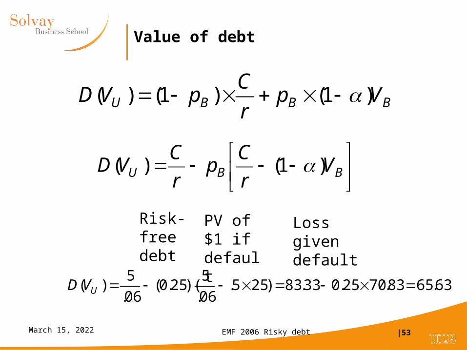
Value of debt

BBU V

r

Cp

r

CVD )1()(

BBBU Vpr

CpVD )1()1()(

Risk-free debt

Loss given default

PV of $1 if default

63.6583.7025.033.83)255.06.

5)(25.0(

06.

5)( UVD


Endogeneous bankruptcy level

• If bankrupcy takes place when market value of equity equals 0:

²)5.0(

)1(

r

CTV C

B

25²)3464.5.06(.

5)0401(

BV


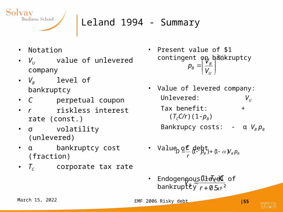
Leland 1994 - Summary

• Notation

• VU value of unlevered company

• VB level of bankruptcy

• C perpetual coupon

• r riskless interest rate (const.)

• σ volatility (unlevered)

• α bankruptcy cost (fraction)

• TC corporate tax rate

• Present value of $1 contingent on bankruptcy

• Value of levered company:

Unlevered: VU

Tax benefit: + (TCC/r)(1-pB)

Bankrupcy costs: - α VB pB

• Value of debt

• Endogeneous level of bankruptcy

BBB pVpr

CD )1()1(

²2

r

U

BB V

Vp

²5.0

)1(

r

CTV C

B


Inside the model

• Value of claim on the firm: F(VU,t)

• Black-Scholes-Merton: solution of partial differential equation

•

• When non time dependence ( ), ordinary differential equation with general solution:

F = A0 + A1V + A2 V-X with X = 2r/σ²

• Constants A0, A1 and A2 determined by boundary conditions:

• At V = VB : D = (1 – α) VB

• At V→∞ : D→ C/r

CrFFVFrVF VVUVUt "'' ²²5.0

0' tF


Unprotected and protected debt

• Unprotected debt:

• Constant coupon

• Bankruptcy if V = VB

• Endogeneous bankruptcy level: when equity falls to zero

• Protected debt:

• Bankruptcy if V = principal value of debt D0

• Interpretation: continuously renewed line of credit (short-term financing)


The Pecking Order Theory

• Developed by S. Myers (1984)

• Starts with asymmetric information:

• Managers know more than outside investors

– Use equity if stock overvalued

– Use debt if stock undervalued

• Issuing equity is a signal of overvaluation =>stock price drops

• Main implication: stock issues costly

• Order of preference for financing:

• 1.Internal funds

• 2. Debt

• 3. Stock issue

Consider the following story:

The announcement of a stock issue drives down the stock price because investors believe managers are more likely to issue when shares are overpriced.

Therefore firms prefer internal finance since funds can be raised without sending adverse signals.

If external finance is required, firms issue debt first and equity as a last resort.

The most profitable firms borrow less not because they have lower target debt ratios but because they don't need external finance.


Implications of the pecking order theory

• Firms do not have target debt ratios

• Debt absorbs difference between retained earnings and investments

• Debt increases when investments > retained earnings

• Debt decreases when investments < retained earnings


The message from CFO’s: debt

What factors affect how you choose the appropriate amount of debt for your firm?Source: US Graham and Harvey J FE December 2001 n = 392

Europe Bancel and Mittoo The Determinants of Capital Structure Choice: A Survey of European Firms, WP 2002

0.00% 10.00% 20.00% 30.00% 40.00% 50.00% 60.00% 70.00% 80.00% 90.00% 100.00%

Potential costs of financial distress

Debt level of other firms in industry

Transactions costs for issuing debt

Tax advantage of interest deductibility

Volatility of earnings and cash flows

Credit rating

Financial flexibility

% important or very important

Europe

US


Survey evidence and capital structure theories

• Trade-off theory Corporate interest deduction

moderately important Cash flow volatility important 44% have strict or somewhat

strict target/range

But: Expected distressed costs not

important Personal taxes not important

• Pecking order theory Firm value flexibility Issue debt when internal funds

are insufficient Equity issuance affected by

equity undervaluation

But: Equity issuance decision

unaffected by ability to obtain funds from debt,…

Debt issuance unaffected by equity valuation


Event studies

Security Issued

Security Retired

Two-Day Announcement Period

Retun

Leverage Increased

Stock Repurchase Debt Common 21.9%

Exchange offer Debt Common 14.0%

Exchange offer Preferred Common 8.3%

Leverage reduced

Exchange offer Common Debt -9.9%

Security Sales Common Debt -4.2%

Conversion-forcing call Common Convertible -0.4%

Conversion-forcing call Common Preferred -2.1%Source: Smith, C. Raising Capital: Theory and Evidence

Against tradeoff story


Problems with empirical studies

• Require data basis + computing capacities

• Accounting convention obscure relevant variables

• Problem for isolating capital structure decisions from other decisions

• Which econometric techniques to use?

• What are the testable hypothesis?

• How to measure the relevant variables?

• Contradictory results

• Harris & Ravis (1990) “The second major trend in financial structure has been the secular increase in leverage.” (p.331)

• Barclay, Smith, Watts (1995) “When viewed over the entire 30-year period, however, both market leverage ratios and dividend yields appear to be remarkably stable.” (p. 5)


Rajan Zingales 1995

• International data – 1987-1991

• Large listed companies

• Difference in accounting rules: pensions, leases

• Do leverage ratios vary across countries?

• Are determinants of leverage identical across countries?


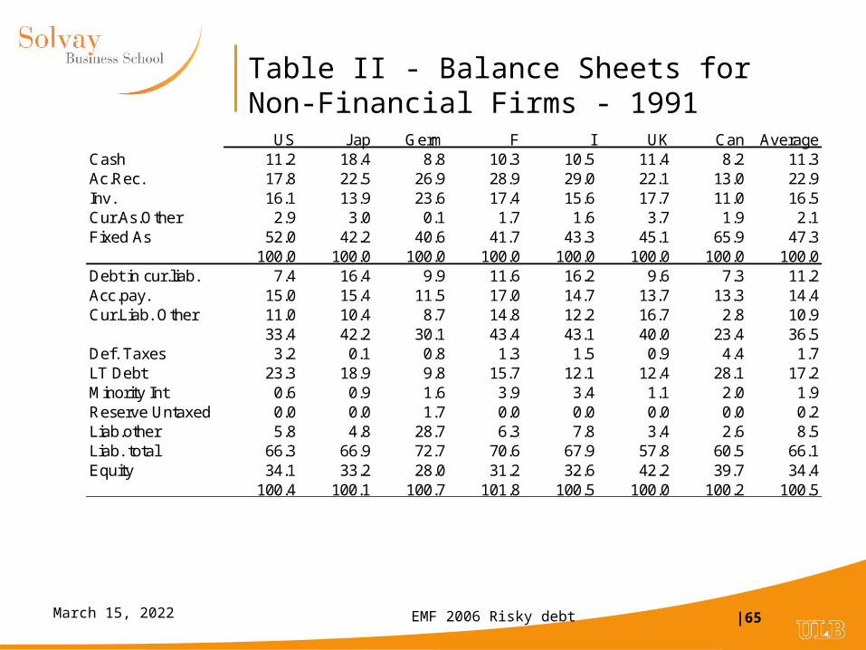
Table II - Balance Sheets for Non-Financial Firms - 1991

US J ap Germ F I UK Can AverageCash 11.2 18.4 8.8 10.3 10.5 11.4 8.2 11.3Ac.Rec. 17.8 22.5 26.9 28.9 29.0 22.1 13.0 22.9Inv. 16.1 13.9 23.6 17.4 15.6 17.7 11.0 16.5Cur.As.Other 2.9 3.0 0.1 1.7 1.6 3.7 1.9 2.1Fixed As 52.0 42.2 40.6 41.7 43.3 45.1 65.9 47.3

100.0 100.0 100.0 100.0 100.0 100.0 100.0 100.0Debt in cur.liab. 7.4 16.4 9.9 11.6 16.2 9.6 7.3 11.2Acc.pay. 15.0 15.4 11.5 17.0 14.7 13.7 13.3 14.4Cur.Liab. Other 11.0 10.4 8.7 14.8 12.2 16.7 2.8 10.9

33.4 42.2 30.1 43.4 43.1 40.0 23.4 36.5Def. Taxes 3.2 0.1 0.8 1.3 1.5 0.9 4.4 1.7LT Debt 23.3 18.9 9.8 15.7 12.1 12.4 28.1 17.2Minority Int 0.6 0.9 1.6 3.9 3.4 1.1 2.0 1.9Reserve Untaxed 0.0 0.0 1.7 0.0 0.0 0.0 0.0 0.2Liab.other 5.8 4.8 28.7 6.3 7.8 3.4 2.6 8.5Liab. total 66.3 66.9 72.7 70.6 67.9 57.8 60.5 66.1Equity 34.1 33.2 28.0 31.2 32.6 42.2 39.7 34.4

100.4 100.1 100.7 101.8 100.5 100.0 100.2 100.5


Table III Leverage in different countries

Book Book adjusted

Market Market adjusted

EBITDA/Interest

United States 37% 33% 28% 23% 4.05x

Japan 53% 37% 29% 17% 4.66x

Germany 38% 18% 23% 15% 6.81x

France 48% 34% 41% 28% 4.35x

Italy 47% 39% 46% 36% 3.24x

United Kingdom 28% 16% 19% 11% 6.44x

Canada 39% 37% 35% 32% 3.05x

Median debt to total capital in 1991

Adjusted debt = Net Debt = Debt – Cash

Book: using book equity, Market: using market value of equity


Determinants of leverage

• Tangibility of assets: Fixed Assets/Total Assets Debt

• Collateral => lower agency cost of debt

• More value in liquidation

• Market to book Debt

• Growth opportunities - underinvestment

• Costs of financial distress

• Size Debt

• Lower probability of bankruptcy

• Less asymmetry of information

• Profitability

• Myers Majluf: profitable companies prefer internal funds


Table IX Factors Correlated with Debt to Market Capital

US J ap Germ F I UK CanTangibility 0.33*** 0.58*** 0.28* 0.18 0.48** 0.27*** 0.11

(0.03) (0.09) (0.17) (0.19) (0.22) (0.06) (0.07)Market-to-book -0.08*** -0.07*** -0.21*** -0.15** -0.18* -.06** -0.13***

(0.01) (0.02) (0.06) (0.06) (0.11) (0.03) (0.03)Logsale 0.03*** 0.07*** -.06*** -0.00 0.04 0.01 0.05***

(0.00) (0.01) (0.02) (0.02) (0.03) (0.01) (0.01)Profitability -0.6*** -2.25*** 0.17 -0.22 -0.95 -0.47** -0.48***

(0.07) (0.32) (0.47) (0.53) (0.77) (0.24) (0.17)

Nb observations 2207 313 176 126 98 544 275

Pseudo R² 0.19 0.14 0.28 0.12 0.19 0.30

Standard errors are in parentheses.*,** and ***, significant at the 10, 5, 1 percent respectively.


References

• Altman, E., Resti, A. and Sironi, A., Analyzing and Explaining Default Recovery Rates, A Report Submitted to ISDA, December 2001

• Bohn, J.R., A Survey of Contingent-Claims Approaches to Risky Debt Valuation, Journal of Risk Finance (Spring 2000) pp. 53-70

• Merton, R. On the Pricing of Corporate Debt: The Risk Structure of Interest Rates Journal of Finance, 29 (May 1974)

• Merton, R. Continuous-Time Finance Basil Blackwell 1990

• Leland, H. Corporate Debt Value, Bond Covenants, and Optimal Capital Structure Journal of Finance 44, 4 (September 1994) pp. 1213-

executive master in finance risky debt professor andré farber solvay business school université...

Documents

b debt

total debt

lt debt

default slide

debt ratio rating classes

wider markets gms debt

bruxelles slide

firm value