Exercise 4:

Samples Characterization

Aim: • Sampling environmental conditions

• Principal Component Analysis of environmental conditions

• Hierarchical clustering of sampling spots

• Interpretation of the environmental dataset

INTRODUCTION

Understanding the complexity of the studied environment represents a crucial aspect of landscape genomics studies. Prior of a study, it is essential to make sure that sufficient variation will be encountered during the sampling campaign. During data interpretation, a representation of how the landscape is structured can strongly support the results analysis. Data Access

We will use all the environmental variables that we collected and produced during the previous exercises. Make sure that they are all contained on the working directory, together with the shapefile with the coordinates of the sheep samples. You can download missing data from the course website. Make sure to have the following files in your working directory:

- The 19 bioclim raster layers - The MAR_urb_30km.tif raster layer - The MAR_slope.tif raster layer - The MAR_hill.tif raster layer - The MAR_alt.vrt raster layer - The CLDsd.tif raster layer - The CLD_mean.tif raster layer - The MOOA_ENV.shp shape file. - The raster layers of your customized variables

You can download missing data from the course website, together with the codes R and python that we will run in this exercise. EXERCISE

Point Sampling of Environmental Conditions Point sampling is the procedure of attributing an environmental value to a point based on his position. QGIS provides a tool that allow to do this in a quick way. Make sure that all the layers we need are loaded on the QGIS project, then click on:

>> Plugins > Analyses > Point Sampling Tool Remember, if you can’t find the Point Sampling Tool you can look up for it in the Plugins Installer. This window will open:

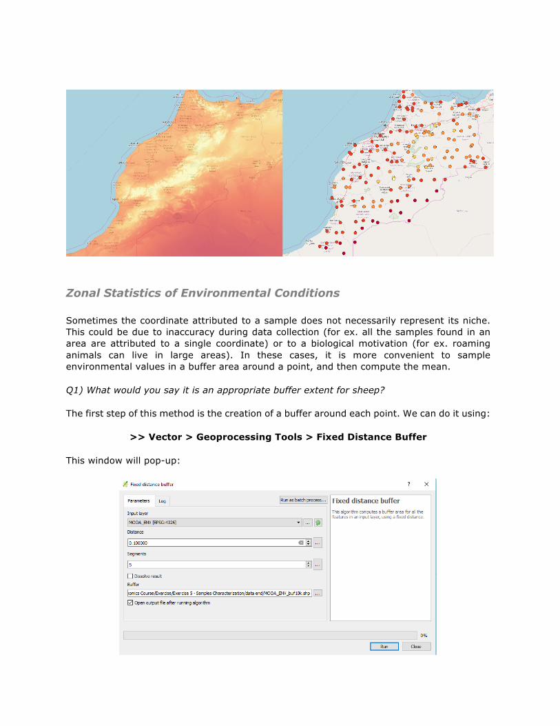
Under Layer containing sampling points, select the MOOA_ENV layer. Then select all the layers you want to sample from by sampling highlighting the layer name. You need to sample from each of the raster file that we prepared and also from the MOOA_ENV, which contains identifiers and coordinates of each sample. Save the new layer as MOOA_ENV_ps.shp. Click on ok. The new layer will appear on the QGIS project. Open the attribute table. You will see that a column per environmental variable was created. Select one variable of interest and compare how the representation of the variable change if we use the raster map or if we use the point samples. Here below it is shown an example for the variable bioclim 1 (Mean Yearly Temperature).

Zonal Statistics of Environmental Conditions Sometimes the coordinate attributed to a sample does not necessarily represent its niche. This could be due to inaccuracy during data collection (for ex. all the samples found in an area are attributed to a single coordinate) or to a biological motivation (for ex. roaming animals can live in large areas). In these cases, it is more convenient to sample environmental values in a buffer area around a point, and then compute the mean. Q1) What would you say it is an appropriate buffer extent for sheep? The first step of this method is the creation of a buffer around each point. We can do it using:

>> Vector > Geoprocessing Tools > Fixed Distance Buffer

This window will pop-up:

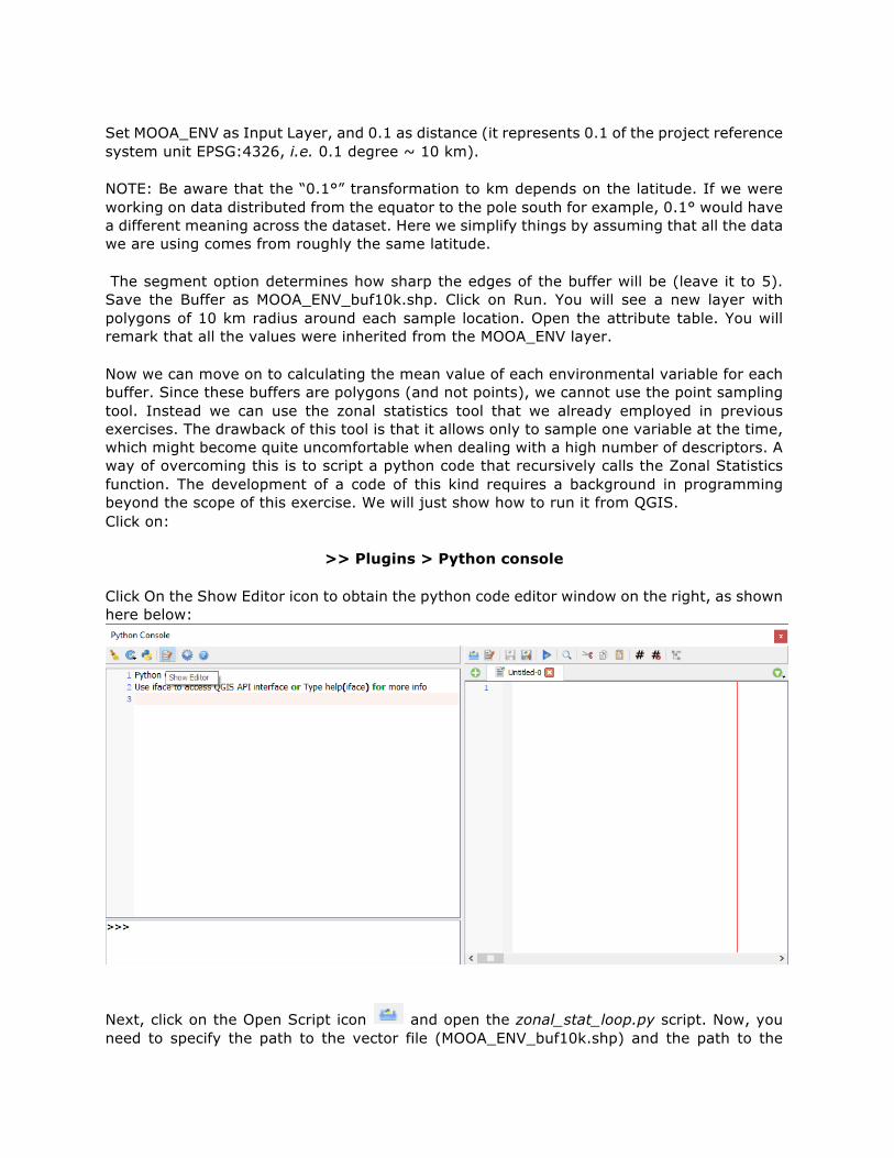
Set MOOA_ENV as Input Layer, and 0.1 as distance (it represents 0.1 of the project reference system unit EPSG:4326, i.e. 0.1 degree ~ 10 km). NOTE: Be aware that the “0.1°” transformation to km depends on the latitude. If we were working on data distributed from the equator to the pole south for example, 0.1° would have a different meaning across the dataset. Here we simplify things by assuming that all the data we are using comes from roughly the same latitude. The segment option determines how sharp the edges of the buffer will be (leave it to 5). Save the Buffer as MOOA_ENV_buf10k.shp. Click on Run. You will see a new layer with polygons of 10 km radius around each sample location. Open the attribute table. You will remark that all the values were inherited from the MOOA_ENV layer. Now we can move on to calculating the mean value of each environmental variable for each buffer. Since these buffers are polygons (and not points), we cannot use the point sampling tool. Instead we can use the zonal statistics tool that we already employed in previous exercises. The drawback of this tool is that it allows only to sample one variable at the time, which might become quite uncomfortable when dealing with a high number of descriptors. A way of overcoming this is to script a python code that recursively calls the Zonal Statistics function. The development of a code of this kind requires a background in programming beyond the scope of this exercise. We will just show how to run it from QGIS. Click on:

>> Plugins > Python console

Click On the Show Editor icon to obtain the python code editor window on the right, as shown here below:

Next, click on the Open Script icon and open the zonal_stat_loop.py script. Now, you need to specify the path to the vector file (MOOA_ENV_buf10k.shp) and the path to the

working directory where all the raster layers are kept. You can retrieve the paths in the General tab of each layer Properties. Once you have modified the paths, click on the Run

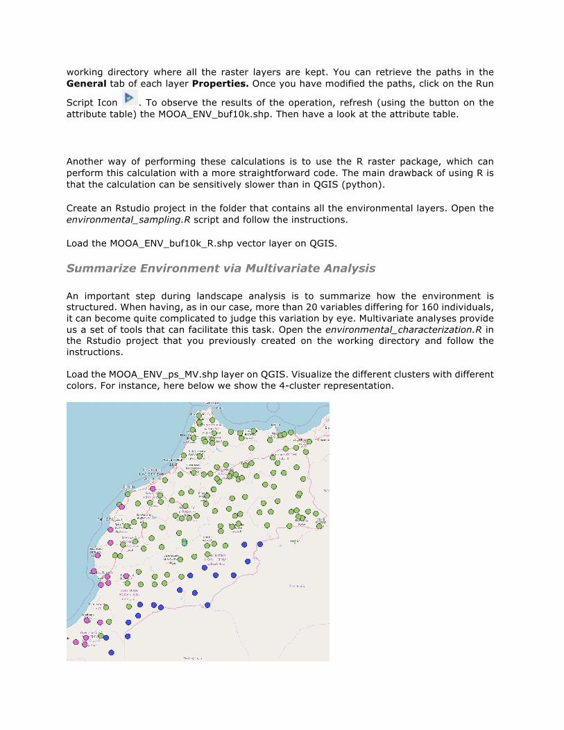
Script Icon . To observe the results of the operation, refresh (using the button on the attribute table) the MOOA_ENV_buf10k.shp. Then have a look at the attribute table. Another way of performing these calculations is to use the R raster package, which can perform this calculation with a more straightforward code. The main drawback of using R is that the calculation can be sensitively slower than in QGIS (python). Create an Rstudio project in the folder that contains all the environmental layers. Open the environmental_sampling.R script and follow the instructions. Load the MOOA_ENV_buf10k_R.shp vector layer on QGIS. Summarize Environment via Multivariate Analysis An important step during landscape analysis is to summarize how the environment is structured. When having, as in our case, more than 20 variables differing for 160 individuals, it can become quite complicated to judge this variation by eye. Multivariate analyses provide us a set of tools that can facilitate this task. Open the environmental_characterization.R in the Rstudio project that you previously created on the working directory and follow the instructions. Load the MOOA_ENV_ps_MV.shp layer on QGIS. Visualize the different clusters with different colors. For instance, here below we show the 4-cluster representation.

Q2) How do the environmental clusters distribute across the study area? What is the meaning of this separation?