Exit Strategies∗

Ignazio Angeloni†

European Central Bank and BRUEGEL

Ester Faia‡

Goethe University Frankfurt, Kiel IfW and CEPREMAP

Roland Winkler§

Goethe University Frankfurt

May 19, 2011

Abstract

We study alternative scenarios for exiting the post-crisis fiscal and monetary accommodationusing the macromodel with banking of Angeloni and Faia (2010) modified and calibrated for theeuro area. The focus is on feasible combinations and tradeoffs between macro performance (out-put and inflation), public debt accumulation and bank stability. Pre-announced and fast fiscalconsolidations dominate – based on simple criteria – alternative strategies incorporating variousdegrees of gradualism and surprise. The fiscal adjustment should be based on spending cuts orelse be relatively skewed towards consumption taxes. The phasing out of monetary accommo-dation should be simultaneous or slightly delayed. We also find that, contrary to widespreadbelief, Basel III may well have an expansionary effect in the long run.

JEL classification: G01, E63, H12Keywords: exit strategies, debt consolidation, fiscal policy, monetary policy, capital require-ments, bank runs

∗An earlier version of this paper was presented at the Banque de France, Goethe University Frankfurt, IndianaUniversity, Universita’ di Roma 2, University of Erlangen-Nuremberg, Dutch National Bank, Bundesbank and Ham-burg University. We are grateful to participants in these conferences and to the staff of the IMF Capital Markets andFiscal Affairs Departments for useful comments. We remain the sole responsible for any errors and for the opinionsexpressed in this paper.

†European Central Bank, Kaiserstrasse 29, Frankfurt am Main, Germany. E-mail: ignazio.angeloni@ecb.int.‡Department of Money and Macro, Grueneburgplatz 1, 60323, Frankfurt am Main, Germany. E-mail:

faia@wiwi.uni-frankfurt.de.§Department of Money and Macro, Grueneburgplatz 1, 60323, Frankfurt am Main, Germany. E-mail:

winkler@hof.uni-frankfurt.de.

1

“By one door you enter, by another you exit”.

PETRONIUS, Satyricon

1st Century AD1

1 Introduction

The more experience we gain with this crisis and its aftershocks, the clearer it becomes that

reversing the policies put in place in response to it and neutralizing their side effects will confront

policy makers with more serious and enduring problems than the crisis itself. Fiscal policy is at the

center of this new challenge. In all industrial countries, public sector deficits expanded sharply since

the second half of 2008 for the combined effect of automatic stabilizers, on both the expenditure

and revenue sides, and discretionary measures to support the financial, corporate and household

sectors. The extent and nature of the official support varied across countries, but the overall effect

was impressive by all standards. Budget deficits increased by about 5 percent of GDP between

2008 and 2009 in both the US and the euro area. Long run simulations by the IMF (see e.g.

Cottarelli and Vinals [21]) show that the debt dynamics will, under favorable circumstances, lead

to increases in public debt ratios in the order of 40 percent or more in the next 6 to 8 years in the

advanced countries; a public debt explosion without precedents in peacetime. An orderly exit from

such imbalance will require sustained consolidation effort for decades, and in the meantime public

finances will remain highly vulnerable to further shocks.

While the fiscal problem is paramount, the question of how to revert the anti-crisis measures

and return to a normal policy setting (the ”exit strategy” problem) is not limited to budgets.

Central banks pegged interest rates close to zero virtually everywhere in late 2008, and a number

of enhanced monetary and credit support programs were enacted. Exiting the monetary expansion

entails a dilemma. On the one hand, delaying the exit helps the recovery and lends a hand to fiscal

sustainability by reducing the interest burden. On the other, however, the exceptionally strong

and protracted monetary expansion encourages risk-taking in the financial sector, as demonstrated

by recent evidence (see a brief survey in Angeloni, Faia and Lo Duca [4]). In the long run, a

1During the reign of Nero (37-68 AD) two unscrupulous fortune-hunters, Encolpius and Ascyltus, travelling insouthern Italy in the company of a young ephebus, Giton, join a banquet offered by the rich libertus Trimalchio.As they later try to leave the extravagant party through the entrance door, they are blocked by the janitor: guestsshould never exit by the same door they entered.

Satyricon is the oldest novel we know of. Only a few fragments have been preserved. Petronius, close adviser andfriend of Nero, was eventually executed by the emperor.

2

protracted monetary expansion can become an obstacle to the restoration of balanced financial

conditions. Moreover, a dilemma arises also in the conduct of financial sector policies, in two

senses. First, publicly funded bank support programs need to be reversed, lest overburdening

public finances and fuelling moral hazard. Second, financial sector reforms, underway in all major

countries under the leadership of the G20, the FSB and the Basel Committee, include as a central

element a strengthening of bank capital. While, on both fronts, action is clearly needed from a

structural viewpoint, excessive frontloading may have undesired cyclical effects, endangering or

delaying the recovery.

In analyzing exit strategies several interconnected factors must be taken into consideration.

The fiscal adjustment is heavily influenced by the timing and modality of monetary exit, but the

reverse is also true, because fiscal consolidation will affect a number of macro-variables that are

in the informational radar screen of central bankers. In addition, the pace of financial reform will

influence how easily and quickly the monetary and liquidity support can be lifted. And so on. That

is why exit strategies should not be examined one at a time, but in combination, and this is also the

reason why a suitably comprehensive analytical framework is so useful to approach the problem2.

In this paper we contribute to this discussion by analyzing and comparing a number of policy

alternatives within a macro-DSGE model that embodies, in a stylised way, all essential ingredients.

While aware of the pitfalls inherent in model-dependent analyses, we believe that the intricacy of

the linkages referred to above can only be approached with the help of a model. Not only one

model, however. Investigating the robustness to alternative modelling structures, while beyond our

ambitions of this paper, is a key development of this research agenda.

We use an adapted version of the model proposed by Angeloni and Faia [3], henceforth AF. AF

integrate a risky banking sector, modelled as in Diamond and Rajan [27], [28] in a standard DSGE

macro framework, and analyse the transmission of monetary and other shocks in an economy with

fragile banks. Banks determine their leverage and balance sheet risk endogenously, influenced by

several factors including the stance of monetary policy; other things equal, a protracted monetary

expansion increases bank leverage and risk. Hence, in addition to the usual channels of monetary

policy, there is also a ”risk-taking” channel, affecting macroeconomic outcomes via the extent of

risk present in the bank balance sheets.

For the purpose of this paper we adjust and extend the AF model in three directions. First, we

add a detailed fiscal sector, including policy functions for public spending, labour and consumption

2The interaction between monetary and fiscal policy is analyzed in our framework within the specification of atype of ”open loop” game and under deterministic setting. This reduces the complexity in terms of the number ofpossible equilibria which can arise.

3

taxes, as well as debt accumulation. This detail is needed to study alternative mixes of fiscal

consolidation strategies and to account for debt dynamics. Second, we augment the bank capital

accumulation equation of the AF model by adding publicly funded bank recapitalisation. This adds

realism to the model, especially in the initial post-crisis phase. Thirdly, we rewrite the model in

linear form in order to apply newly developed methods to analyse and compare complex sequences

of shocks and policy responses, with different timing and informational assumptions. This permits

us to approach questions that are common in many current discussions on exit strategies, such as

gradualism versus preemptive action, sequencing and delay (who should exit first, fiscal or monetary

policy? what is the cost or benefit from delaying?) and communication policy (should the exit

strategy be pre-announced)?

While we are not aware of other papers approaching the issue of exit strategies in the fashion

we do, our paper is closely related to several strands of recent literature. The first is, naturally,

that combining banking, finance and macro modelling and studying the role of monetary policy

in preventing and in managing a financial crisis. The second relevant field of literature is that on

the effects of fiscal policy, including the role of gradualism versus front-loading, announcement, as

well as the tax-expenditure mix of fiscal consolidations. The third is the work on monetary and

fiscal regimes, including the effects of endogenous regime switching. These and other links with the

literature are briefly recapitulated in a section below.

Our main conclusions can be summarized as follows. First and foremost, exiting the post-crisis

policy stance is beneficial; undertaking an exit strategy, almost of any form, leads to an improvement

in terms of our evaluation criteria (intertemporal consumption and output; inflation and bank risk)

relative to the status quo (i.e., the indefinite continuation of the post-crisis accommodative policy

course). Not all exit strategies are alike, though. Active fiscal strategies, geared to an ambitious

debt consolidation target and credibly communicated in advance, dominate gradual, unannounced

ones. The composition of fiscal policy matters. Spending-based fiscal strategies are superior to

tax-based ones in most cases. Among the tax-based ones, strategies tilted towards consumption

taxes perform relatively well. The effect of sequencing (monetary policy moving before fiscal, or

the reverse) are more nuanced. Among active and pre-announced strategies, those where monetary

and fiscal policies move together are almost equivalent to those where fiscal moves first. Strategies

where monetary policy leads are not as effective. We also analyse, in a qualitative way, how our

model economy reacts to the transition to Basel III (the new capital accord recently agreed by the

Basel Committee on Bank Supervision). We find that the ”countercyclical buffer”, a main feature

of the new standard which foresees that banks can release capital in a recession but must build it

up in booms, has a powerful stabilizing macroeconomic effect, as intended. Moreover, and more

4

surprisingly, we find that a permanent increase in bank capitalization can be expansionary in our

model (rather than contractionary, as typically argued) in the long run, for plausible parameter

values. The expansionary effect stems from the increase in the supply of bank capital induced by

regulation, assuming (as we do) that all proceeds of bank capitalists are reinvested.

A unifying message from our results could be stated as follows: a successful exit from the

exceptional post-crisis accommodation requires not a mere return to old policy regimes, but a tran-

sition to a new approach. On the fiscal side, its main ingredients are a more credible commitment

to intertemporal sustainability, more front-loaded adjustment, and clearer communication of long

term targets. On the monetary side, taking into account the effects of central bank action on moral

hazard and risk taking in the financial sector. On financial policies, the explicit consideration of

their macroprudential dimension. Far from being a travel in reverse, the exit from post-crisis poli-

cies offers the chance of, and solicits, a qualitative change of the way macroeconomic policies are

conducted.

The rest of the paper is organized as follows. Section 2 reviews the related literature and

highlights the areas where this paper contributes. Section 3 describes the model and the simulation

methodology we use to study and compare exit strategies. Section 4 describes the calibration of the

model and the policy regimes, and the methodology for designing and simulating the exit strategies.

Section 5 describes our baseline path, which includes two elements: the initial shock (the ”crisis”)

and the immediate policy responses. Our aim here is to formulate a realistic set of impulses that

generate in the model a response in the main macro variables that roughly mimics that observed in

the euro area in the two years following the onset of the financial crisis. The next step, in section

6, is to analyse a number of alternative strategies of exit from fiscal and monetary accommodation

(paths of the main macro variables following alternative combination of changes in the existing

fiscal and monetary rules), and compare their performance against the baseline. To do this we use

visual inspection and quantitative ad hoc criteria. The final step, in section 7, is to examine the

phasing in of Basel III. Finally, section 8 concludes.

2 Links to the literature

In the aftermath of the crisis most of the literature on fiscal and monetary policy focused on

analyzing how effective unconventional monetary and fiscal policy could be in managing the crisis.

In all countries governments have let fiscal automatic stabilizers play with full force and most have

also passed discretionary stimulus packages. Monetary policy has adopted a proactive expansionary

stance, particularly in the US, where, since the aggravation of the crisis in late 2008, the reference

5

interest rate has remained stable at the zero lower bound.

In this context, a number of papers have analyzed the effects of fiscal packages, focusing

particularly on the size of the fiscal multipliers. The first analysis of this type, by authors close to

the Obama administration, is contained in the paper by Romer and Bernstein [45]: those authors

have argued that large fiscal stimuli can be extremely beneficial as fiscal multipliers are significantly

larger than one. Their conclusions have been challenged by several authors, who have published

estimates of the fiscal multipliers suggesting far less favorable scenarios (see Cogan et al. [18], Cwik

and Wieland [23], Uhlig [49] among others). Christiano, Eichenbaum and Rebelo [17] argue that

fiscal multipliers might be larger than one when the interest rate is at the zero lower bound. On

the effects of government spending on the macroeconomy there is also a vast VAR-based literature,

which however is only marginally related to our paper.

In the US much of the discussion has focused on how the Federal Reserve should reabsorb

liquidity avoiding inflationary pressure. The paper by Gertler and Karadi [32] considers the effects

of ”news shocks” for the case in which the monetary authority decides to abandon unconventional

measures. A recent paper by Chari [15] analyzes three alternative strategies for draining reserves:

(1) paying interest on excess reserves, (2) managing interest rates on short-term deposits, and (3)

selling back financial assets such as mortgage-backed securities. He concludes that the best course

would be a blend of the three.

Our paper is also related to the literature on policy regimes. Davig and Leeper [25] estimates

Markov-switching policy rules for the United States and finds that monetary and fiscal policies

fluctuate between active and passive behavior. Davig, Leeper and Walker [26] apply the same

framework to study the consequences of alternative means to resolve the “unfunded liabilities”

problem—the projected exponential growth in federal Social Security, Medicare, and Medicaid

spending with no known plan for financing the transfers. Aside from the literature on discretionary

policy in which changing policy in every periods involves game theoretic interactions between

agents and government, standard DSGE models could not so far accommodate unexpected change

in policy: a recent methodology developed by Juillard [37] takes important steps in this direction.

As the model we use introduces banks into DSGE models, our paper is also related to the

recent literature on this topic, which includes Gertler and Karadi [32], Gertler and Kiyotaki [33],

Meh and Moran [41], Covas and Fujita [22], He and Krishnamurthy [34], Bunnermeier and Sannikov

[12], Gerali et al. [31], Angelini et al. [2], Darrein Paries et al. [24].

Finally, our paper is related to recent work by Corsetti et al. [20] which analyzes the effects of

fiscal stimulus and fiscal exit in deep recessions when the interest rate is at the zero lower bound.

They show, by using a standard New Keynesian model without banks, that debt consolidation

6

through the credible announcement of future spending cuts generally amplifies the expansionary

effects of a fiscal stimulus.

3 The Model

The starting point is the model developed in AF [3] who introduce banks following Diamond and

Rajan [27], [28] into a conventional DSGE model with nominal rigidities. To this we add a fiscal

sector which sets government expenditure following an operational rule which responds to past

spending and government debt. Government spending is financed through a mix of labour and

consumption taxes and government debt. Monetary policy follows a standard Taylor rule in the

baseline scenario.

There are five type of agents in this economy: households, financial intermediaries, non-

financial good producers, capital producers and monopolistic firms. Financial intermediaries fund

projects by raising money from depositors3 and bank capitalists. Projects are subject to an id-

iosyncratic shock, which generates the possibility of bank runs. As in Diamond and Rajan [27], [28]

the bank capital structure is determined by bank managers, who act on behalf of outside investors

(depositors and bank capitalists combined) by maximizing their overall return. Once the project’s

uncertain outcome is realized, bank capitalists claim the residual value after depositors are paid out.

If the return on bank assets is low and the bank is not able to pay depositors in full there is a run

on the bank, in which case the bank capital holders get zero while depositors get the market value

of the liquidated loan. Finally, we assume that monopolistic firms in the production sector face

quadratic adjustment costs on prices: such an assumption allows to generate non-neutral effects of

monetary policy.

3.1 Households

There is a continuum of identical households who consume, save and work. Households save by

lending funds to the financial intermediaries, both in the form of deposits and bank capital. To allow

aggregation within a representative agent framework we follow Gertler and Karadi [32] and assume

that in every period a fraction γ of household members are bank capitalists and a fraction (1− γ)

are workers/depositors. Hence households also own financial intermediaries4. Bank capitalists

remain engaged in their business activity next period with a probability θ, which is independent of

3As in Diamond and Rajan [27] we need to clarify that demand deposits represent more generally short termliabilities subject to service constraints, a concept which includes asset backed securities, an asset subject to run inthe form of liquidity dry-ups in the current crisis.

4As in Gertler and Karadi [32] it is assumed that households hold deposits with financial intermediaries that theydo not own.

7

history. This finite survival scheme is needed to avoid that bankers accumulate enough wealth to

ease up the liquidity constraint. According to this structure a fraction (1− θ) of bank capitalists

exit in every period. A corresponding fraction of workers become bank capitalists every period,

so that the share of bank capitalists, γ, remains constant over time. Workers earn wages5 and

return them to the household; similarly bank capitalists return their earnings to the households.

However, bank capitalists earnings are not used for consumption but are given to the new bank

capitalists and reinvested as bank capital. Consumption and investment decisions are made by

the household, pooling all available resources. Bank managers, who determine the bank capital

structure, are simply workers in the financial sector. Household members can either work in the

production sector or in the financial sector. We assume that the fraction of workers in the financial

sector is negligible, hence their wage earnings are not included in the budget constraint.

Households maximizes the following discounted sum of utilities

E0

∞∑

t=0

βt(

1

1− σ(Ct − γCa

t−1)1−σ + ν log(1−Nt)

)

(1)

where Ct denotes consumption, Cat−1 denotes aggregate past consumption, and Nt denotes labour

hours. The introduction of habit persistence in consumption through the dependence of the utility

from past aggregate consumption smooths out fluctuations in consumption, thereby rendering its

path empirically more plausible. Households save and invest in government bonds, Bt, bank de-

posits, Dt, and bank capital. Deposits and government bonds pay a gross nominal return Rt one

period later. Finally, households are also the owners of the monopolistic competitive sector, hence

they receive real profits for an amount, Θt. The budget constraint reads as follows:

(1 + τ ct )Ct +Bt

Pt+Dt

Pt= (1− τnt )

Wt

PtNt +Rt−1

Bt−1

Pt+Rt−1

Dt−1

Pt+ τt +Θt

where τ ct and τnt are taxes on consumption purchases and labour income, respectively. τt denotes

a lump-sum transfer.6

5Workers are employed in the real or in the financial sector, as bank managers. Bank managers, a small fractionof existing workers, receive a fee (for the latter, see the next section). We do not include this fee in the budgetconstraint for simplicity, assuming it is insured away and embodied in the wages of the production sector.

6We assume away, for simplicity, risk premia on deposits and on government bonds. The first would stem fromthe risk of run. In essence we assume that households pool resources to insure against such shocks. The insurancecontract, however, guarantees only the residual deposit unpaid by the bank; hence a bank run must occur for theinsurance compensation to be paid. The second issue is potentially more important in the context of this paper.It is realistic to assume that ambitious fiscal consolidations dampen sovereign risk spreads, hence dampening theaccumulation of debt and elevating the long-term benefits of fiscal consolidation further. In this respect our paperprobably underestimates the effect of ambitious fiscal exit strategies. We leave the inclusion of endogenous bondspreads to future work.

8

The following optimality conditions (alongside with a No-Ponzi conditions) hold after aggre-

gation:

λt = (Ct − γCt−1)−σ 1

1 + τ ct(2)

λt = βEt

{

λt+1Rt

πt+1

}

(3)

Wt

Pt= ν [(1−Nt)λt(1− τnt )]

−1 (4)

3.2 Banks

There is in the economy a large number (Lt) of uncorrelated investment projects. The project lasts

two periods and requires an initial investment. Each project’s size is normalized to unity (think of

one machine) and its price is Qt. The projects require funds, that are provided by the bank. Banks

have no internal funds but receive finance from two classes of agents: holders of demand deposits

and bank capitalists. Total bank loans (equal to the number of projects multiplied by their unit

price) are equal to the sum of deposits (Dt) and bank capital (BKt). The aggregate bank balance

sheet is:

QtLt = Dt +BKt (5)

The capital structure (deposit share, equal to one minus the capital share) is determined by

bank manager on behalf of the external financiers (depositors and bank capitalists). The manager’s

task is to find the capital structure that maximizes the combined expected return of depositors

and capitalists, in exchange for a fee. Individual depositors are served sequentially and fully as

they come to the bank for withdrawal; bank capitalists instead are rewarded pro-quota after all

depositors are served. This payoff mechanism exposes the bank to runs, that occur when the return

from the project is insufficient to reimburse all depositors; as soon as they realize that the payoff

is insufficient, they run the bank and force the liquidation of the project. The timing is as follows.

At time t, the manager of bank k decides the optimal capital structure, expressed by the ratio of

deposits to total loans, dk,t =Dk,t

Qk,tLk,t, collects the funds, lends, and then the project is undertaken.

At time t + 1, the project’s outcome is known and payments to depositors and bank capitalists

(including the fee for the bank manager) are made, as discussed below. A new round of projects

starts.

Generalizing Diamond and Rajan [27], [28], we assume that the return of each project for the

bank is equal to an expected value, RA,t, plus a random shock, for simplicity assumed to have a

uniform density with dispersion h (the assumption yields a convenient closed form solution but is

9

not essential; see AF [3] for the case of logistic and normal distributions). Therefore, the project j

outcome is RA,t + xj,t, where xj,t spans across the interval [−h;h] with probability 12h . We assume

h to be constant across projects.

Given our assumption of identical projects and banks, for notational convenience from now

on we can omit project and bank subscripts. Until the end of this subsection we will omit time

subscript as well.

Each project is financed by one bank. Our bank is a relationship lender : by lending it acquires

a specialized non-sellable knowledge of the characteristics of the project. This knowledge determines

an advantage in extracting value from it before the project is concluded, relative to other agents.

Let the ratio of the value for the outsider (liquidation value) to the value for the bank be 0 < λ < 1.

Again we assume λ to be constant.

Suppose the ex-post realization of x is negative and consider how the payoffs of the three

players are distributed depending on the ex-ante determined value of the deposit ratio d and the

deposit rate R. There are three cases.

Case A: Run for sure. The outcome of the project is too low to pay depositors. This happens

if RA + x < Rd. Payoffs in case of run are distributed as follows. Capitalists receive the leftover

after depositors are served, so they get zero in this case. Depositors alone (without bank) would

get only a fraction λ(RA + x) of the project’s outcome; the remainder (1 − λ)(RA + x) is shared

between depositors and the bank depending on their relative bargaining power. We assume this

extra return is split in half (other assumptions are possible without qualitative change in the

results7). Therefore, depositors end up with

(1 + λ)(RA + x)

2

and the bank with(1− λ)(RA + x)

2(6)

Case B: Run only without the bank. The project outcome is high enough to allow depositors

to be served if the project’s value is extracted by the bank, but not otherwise. This happens if

λ(RA + x) < Rd ≤ (RA + x). In this case, the capitalists alone cannot avoid the run, but with the

bank they can. So depositors are paid in full, Rd, and the remainder is split in half between the

banker and the capitalists, each getting RA+x−Rd2 . Total payment to outsiders is RA+x+Rd

2 .

7Depositors and bank managers have equal bargaining power because neither can appropriate the extra rentwithout help from the other. Diamond and Rajan [27] mention also another case in which the depositors, afterappropriating the project, bargain directly with the entrepreneur running the project. If the entrepreneur retainshalf of the rent, the result is obviously unchanged. If not, the resulting equilibrium is more tilted towards a highlevel of deposits, because depositors lose less in case of bank run.

10

Case C: No run for sure. The project’s outcome is high enough to allow all depositors to be

served, with or without the bank’s participation. This happens if Rd ≤ λ(RA + x). Depositors

get Rd. However, unlike in the previous case, now the capitalists have a higher bargaining power

because they could decide to liquidate the project alone and pay the depositors in full, getting

λ(RA + x) − Rd; this is thus a lower threshold for them. The banker can extract (RA + x) − Rd,

and again we assume that the capitalist and the bank split this extra return in half. Therefore, the

bank gets:[(RA + x)−Rd]− [λ(RA + x)−Rd]

2=

(1− λ)(RA + x)

2

This is less than what the capitalist gets. Total payment to outsiders is:

(1 + λ)(RA + x)

2

We can now write the expected value of total payments to outsiders as follows:

1

2h

Rd−RA∫

−h

(1 + λ)(RA + x)

2dx+

1

2h

Rdλ

−RA∫

Rd−RA

(RA + x) +Rd

2dx+ (7)

+1

2h

h∫

Rdλ

−RA

(1 + λ)(RA + x)

2dx

The three terms express the payoffs to outsiders in the three cases described above, in order.

The banker’s problem is to maximize expected total payments to outsiders by choosing the suitable

value of d.

The solution to the above maximization yields the following solution for the level of deposits

for each unit of loans:

d =1

R

RA + h

2− λ. (8)

Since the second derivative is negative, this is the optimal value of d. For analytical details

characterizing the solution the reader is referred to the paper by AF [3]. In their paper the

authors also show that the above result holds for a variety of assumptions also in terms of different

probability distribution for the underlying idiosyncratic shock.

We can measure bank riskiness by the probability of a run occurring. This can be written as:

brt =1

2h

Rd−RA∫

−h

dx =1

2

(

1−RA −Rd

h

)

=1

2−RA(1− λ)− h

2h(2− λ)(9)

11

The Risk Taking Channel

To guide the interpretation of our later results concerning the exit strategies, some considerations

are in order on the relation between the interest rate and the deposit ratio on one side, and the

probability of run on the other. In the decision about whether/when to exit, there is a trade-off

between the short run benefits of expansionary policies and their long run costs. The short run

benefits are clear: using a sticky price model, lowering the interest rate results in expansion of

aggregate demand and output. As for the long run costs, one of them, and the most important, is

the effect of changes in the interest rate on the optimal deposit ratio. In this respect the features

characterizing our banking model become crucial. The model features a risk taking channel, namely

the fact that low interest rates fuel banking risks. At low interest rates banks tends to fund

themselves with deposit liabilities, therefore increasing the probability runs and bank riskiness.

This can be seen by inspecting equation 8. Even though in the general equilibrium a fall in Rt

triggers a fall in RA,t, the risk premium, represented by the ratioRA,t

Rt, decreases, therefore inducing

an increase d. The increase in the risk premium triggers a fall in asset prices and investment. In

presence of such channel, expansionary policy might in the long run might depress output relatively

to the case in which the above mentioned channel is absent.

Accumulation of bank capital and bank recapitalization

In the aggregate, the amount invested in every period is QtLt. The total amount of deposits in the

economy is

Dt =QtLt

Rt

RA,t + h

2− λ(10)

and the bank’s optimal capital is:

BKt = (1−1

Rt

RA,t + h

2− λ)QtLt (11)

Projects are financed by the intermediary for an amount:

QtLt = QtKt (12)

The above expressions suggest that following an increase in Rt the optimal amount of bank

capital increases on impact (for given RA,t). The effect of other factors in general equilibrium is

more complex, depending on several counterbalancing factors affecting RA,t and Rt, as the later

results will show.

12

Equation 11 is the level of bank capital desired by the bank manager, for any given level of

investment, QtLt and interest rate structure (Rt, RA,t). We assume that bank capital is provided

by the bank capitalist. After remunerating depositors and paying the competitive fee to the bank

manager, a return accrues to the bank capitalist, and this is reinvested in the bank as follows:

BKt = θ[BKt−1 +RTKtQtKt] (13)

where RTKt is the unitary return to the capitalist. The parameter θ is a decay rate, given by the

bank survival rate already discussed. RTKt can be derived as follows:

RTKt =1

2h

h∫

Rtdt−RA,t

(RA,t + x)−Rtdt2

dxt =(RA,t + h−Rtdt)

2

8h(14)

Note that this expression considers only the no-run state because if a run occurs the capitalist

receives no return. The accumulation of bank capital is obtained substituting 14 into 13:

BKt = θ[BKt−1 +(RA,t + h−Rtdt)

2

8hQtKt] (15)

In face of a crisis scenario banks also receive some transfers in the form of bank recapitalization,

BKGt. Hence the above equation now reads as follows:

BKt = θ(BKt−1 +RTKQtKt) +BKGt

3.3 Producers

Each firm i has monopolistic power in the production of its own variety and therefore has leverage

in setting the price. In changing prices it faces a quadratic cost equal to ϑ2 (

Pt(i)Pt−1(i)

− 1)2, where

the parameter ϑ measures the degree of nominal price rigidity. The higher ϑ the more sluggish

is the adjustment of nominal prices. In the particular case of ϑ = 0, prices are flexible. Each

firm assembles labour (supplied by the workers) and (finished) entrepreneurial capital to operate a

constant return to scale production function for the variety i of the intermediate good:

Yt(i) = AtF (Nt(i), Kt(i)) (16)

Each monopolistic firm chooses a sequence {Kt(i), Lt(i), Pt(i)}, taking nominal wage rates

Wt and the rental rate of capital Zt, as given, in order to maximize expected discounted nominal

profits:

13

E0{∞∑

t=0

Λ0,t[Pt(i)Yt(i)− (WtNt(i) + ZtKt(i))−ϑ

2

[

Pt(i)

Pt−1(i)− 1

]2

Pt]} (17)

subject to the constraint AtFt(•) ≤ Yt(i), where Λ0,t is the households’ stochastic discount factor.

Let’s denote by {mct}∞t=0 the sequence of Lagrange multipliers on the above demand constraint.

The following first order conditions for profit maximization hold (after aggregation):

Wt

Pt= mctAtFN,t (18)

Zt

Pt= mctAtFK,t (19)

Uc,t(πt − 1)πt = βEt{Uc,t+1(πt+1 − 1)πt+1}+ Uc,tAtFt(•)ε

ϑ(mct −

ε− 1

ε) (20)

The latter equation is a non-linear forward looking New-Keynesian Phillips curve, in which

deviations of the real marginal cost from its desired steady state value are the driving force of

inflation (Woodford [50]).

3.4 Capital sector

A competitive sector of capital producers combines investment (expressed in the same composite

as the final good, hence with price Pt) and existing capital stock to produce new capital goods.

This activity entails physical adjustment costs. Such costs are modelled so as to mimic correctly

the initial drop in investment under the crisis scenario. First, capital adjustment costs depend on

the change in investment according to the following equation:

CACt = S

(

ItIt−1

)

It (21)

where S(1) = 0 and S′(1) = 0. The capital accumulation equation is then given by:

Kt+1 = Kt(1− δ) +

[

1− S

(

ItIt−1

)]

It (22)

Second, we also consider variable capital utilization. Producers use Kt = utKt, which is the effective

utilization of the capital stock. The capital utilization rate is determined endogenously. The capital

producer maximizes real profitsZt

PtutKt − It −Ψ(ut)Kt (23)

subject to the capital accumulation equation. Notice that Ψ(ut)Kt are costs associated with vari-

ations in the degree of capital utilization. The first order conditions for profit maximization read

14

as:

RA,t+1

πt+1=

(

Zt+1

Pt+1ut+1 −Ψ(ut+1) +Qt+1(1− δ)

)

Qt(24)

Qt

(

1− S

(

ItIt−1

))

= QtS′

(

ItIt−1

)(

ItIt−1

)

−πt+1

RA,t+1Qt+1S

′

(

It+1

It

)(

It+1

It

)2

+ 1 (25)

Zt

Pt= Ψ′(ut) (26)

3.5 Equilibrium conditions

Equilibrium in the final good market requires that the production of the final good equals the sum

of private consumption by households, investment, public spending, and the resource costs that

originate from the adjustment of prices and capital:

Yt = Ct + It +Gt +Ψ(ut)Kt +ϑ

2(πt − 1)2 (27)

3.6 Monetary Policy and the Fiscal Sector

Monetary policy is represented by an interest rate reaction function of this form:

ln

(

Rt

R

)

= (1− φr)

[

φπ ln(πtπ

)

+ φy ln

(

YtY

)]

+ φr ln

(

Rt−1

R

)

(28)

All variables are deviations from the target or steady state (symbols without time subscript).

Fiscal policy is also described by feedback rules that determine government spending, real

government debt Brt = Bt/Pt and the composition of taxes. In order to pin down to which extent

an increase in government spending is financed by raising consumption and /or labour taxes or by

issuing new bonds, we follow Uhlig [49] and consider a rule of the following form

ln

(

τntτn

)

+ ln

(

τ ctτ c

)

= ψT

[

ln

(

Brt

Br

)

+ ln

(

τntτn

)

+ ln

(

τ ctτ c

)]

(29)

For ψT = 1 an increase in government spending is solely tax-financed leaving real government debt

unchanged. On the contrary, for ψT = 0 an increase in government spending is completely financed

by new debt.

The composition of taxes is determined with the help of the following tax rule:

ln

(

τntτn

)

= ψτ

[

ln

(

τntτn

)

+ ln

(

τ ctτ c

)]

(30)

The parameter ψτ determines to which extent tax financing is done by raising labour taxes τnt

instead of consumption taxes τ ct . Notice that the limiting case ψτ = 0 implies that the direct

15

(labour) tax rate sticks to its steady state value and tax financing is done solely by raising indirect

(consumption) taxes. For ψτ = 1, tax financing is completely shifted to labour taxes leaving

consumption taxes unchanged.

Finally, we follow Corsetti, Meier and Muller [19] and consider the following government

spending rule

ln

(

Gt

G

)

= ρg ln

(

Gt−1

G

)

− γB ln

(

Brt

Br

)

+ εgt (31)

where εgt is an exogenous shock. The parameter γB measures the strength of the endogenous

response of government spending to debt.

The government budget constraint which closes the fiscal side of the economy is given by

Brt =

Rt−1

πtBr

t−1 +Gt +BKGt − τ ct Ct − τntWt

PtNt + τt (32)

4 Calibration

Preferences and production. Time is measured in quarters. We set the intertemporal elasticity

of consumption to σ = 1.4 which is roughly the value estimated by Smets and Wouters [47] for

the Euro area. We calibrate the elasticity of labour supply, ν, to 1.425 as this induces a steady

state number of hours worked of 0.3. As it is standard in New Keynesian models we calibrate the

elasticity of demand, ε, to 6 as this induces a mark-up of 1.2. The discount factor is calibrated to

0.99 so that the annual interest rate is 4%. Following Smets and Wouters [47] we set the degree of

habit formation, γ, to 0.5.

We assume a Cobb-Douglas production function F (•) = KαN1−α, with α = 1/3. The quarterly

aggregate capital depreciation rate δ is 0.025. Following Smets and Wouters [47] the adjustment

cost parameter, φI = 1/S′′, is set to 1/6, while the utilization cost parameter, φu = Ψ′/Ψ′′, is set

to 1/0.2.

In order to parameterize the degree of price stickiness ϑ, we observe that by log-linearizing

equation 18 we can obtain an elasticity of inflation to real marginal cost (normalized by the steady-

state level of output)8 that takes the form ε−1ϑ. This allows a direct comparison with empirical

studies on the New-Keynesian Phillips curve such as Gali and Gertler [30] and Sbordone [46] using

Calvo-Yun approach. In those studies, the slope coefficient of the log-linear Phillips curve can be

expressed as (1−ϑ)(1−βϑ)

ϑ, where ϑ is the probability of not resetting the price in any given period

in the Calvo-Yun model. For any given values of ε, which entails a choice of the steady state

8To produce a slope coefficient directly comparable to the empirical literature on the New Keynesian Phillips curvethis elasticity needs to be normalized by the level of output when the price adjustement cost factor is not explicitlyproportional to output, as assumed here.

16

level of the markup, we can thus build a mapping between the frequency of price adjustment in

the Calvo-Yun model 11−ϑ

and the degree of price stickiness ϑ in the Rotemberg setup. The recent

New Keynesian literature has usually considered a frequency of price adjustment of four quarters as

realistic. Recently, Bils and Klenow [8] have argued that the observed frequency of price adjustment

in the US is higher, in the order of two quarters. As a benchmark we use a slightly higher value

consistent with the estimates of Smets and Wouters [47] and parameterize 11−ϑ

= 5, which implies

ϑ = 0.8. Given ε = 6, the resulting stickiness parameter satisfies ϑ = Y ϑ(ε−1)

(1−ϑ)(1−βϑ)≈ 30, where Y is

steady-state output.

Bank parameters. To calibrate h we have calculated the average dispersion of corporate returns

from the data constructed by Bloom et al. [10], which is around 0.3, and multiplied this by the

square root of 3, the ratio of the maximum deviation to the standard deviation of a uniform

distribution. The result is 0.5. We set the value of h slightly lower, at 0.45, a number that yields

a more accurate estimate of the steady state value of the bank deposit ratio.9

One way to interpret λ is to see it as the ratio of two present values of the project, the first at the

interest rate applied to firms’ external finance, the second discounted at the bank internal finance

rate (the money market rate). A benchmark estimate can be obtained by taking the historical ratio

between the money market rate and the lending rate. In the US over the last 20 years, based on

30-year mortgage loans, this ratio has been around 3 percent. This leads to a value of λ around

0.6. In the empirical analyses we have chosen 0.45. Finally we parameterize the survival rate of

banks at 0.97.

Fiscal policy parameters. The constant fraction of public spending, G is calibrated so as

to match G/Y = 0.23. Steady state taxes are set to τ c = 0.17 and τn = 0.41 which are values

calculated for the euro area by Trabandt and Uhlig [48]. The steady state value of government

debt is set to Br/Y = 0.7.

For the initial crises scenario, the fiscal feedback rules are calibrated as follows. ψτ is set to

2/3 implying a mix of direct and indirect taxes consistent with the composition of taxes in the Euro

area.10 The responsiveness of government spending to debt is set to γB = 0 implying, as standard

9The bank capital accumulation equation 13, once we substitute in the optimal deposit ratio 10, and the returnaccruing to the bank capitalist 14, yields a quadratic equation in RA. Solving the quadratic equation for given valuesof the parameters, one obtains a root for RA equal to 1.03 (3 percent on a quarterly basis). The corresponding valueof d is 95 percent, and bk is 5 percent. Notice that the bank capital accumulation equation includes the money thathouseholds transfer in every period to new bankers, given by a fraction of the value of the project: φQtKt. Thesteady state value that helps to pin down the return on asset, RA, is 0.075. Since such term is negligible we haveomitted that in the dynamic.

10Notice that total fiscal revenues in the euro area are about 45 percent of GDP, of which about two thirds arecomposed by direct taxes and social security contribution on individuals and corporations. The remaining fractionis indirect taxes. Both direct taxes and social security contributions can be regarded as labour-related levies.

17

in most of the literature, an exogenous process for government spending. The autocorrelation of

government spending is assumed to be 0.9 which is consistent with the estimates by Smets and

Wouters [47] for the Euro area. The value ψT = 0.1 ensures the dynamic stability of public debt,

but only in the very long run.

Monetary policy parameters. We distinguish between passive and active monetary policy.

Passive monetary policy means that the nominal interest rate is fixed at its steady state value

Rt = R. In order to ensure determinacy, the monetary authority must credibly announce a future

exit from this passive policy and a switch to an active feedback rule. This feedback rule is equation

28 with a coefficient on inflation, φp, equal to 1.5 and a coefficient on output, φy, equal to 0.5/4.

The parameter φr is set equal to zero in the baseline calibration.

4.1 Constructing the exit strategies

Our simulation strategy is as follows. We first construct a baseline scenario that mimics the actual

situation experienced during the 2007-2008 crisis (see details in the next section). Then, starting

from this scenario, we calculate the effects of different combination of exit strategies in terms of

both, monetary and fiscal policy. Alternative monetary and fiscal exit strategies differ with respect

to the degree of activism, the sequencing of events, and the composition of fiscal adjustment. We

also distinguish between policy changes that are credibly pre-announced and policy changes that

happen unexpectedly.

Monetary policy. We assume that a switch from passive to active monetary policy takes place

when there is an upward pressure on prices. Technically, we compute the expected path of the

nominal interest rates under different credibly announced exit dates, with fiscal policy as in our

baseline case. We then find the date when the Taylor rule calls for an increase in the nominal

interest rate. Under our baseline calibration and under the baseline crisis scenario, discussed in the

next section, this date is t = 13 (after three years). We call this an announced monetary exit. We

also consider an unanticipated monetary exit. In this case, the monetary exit that is announced to

happen at t = 13, unexpectedly happens one year earlier, i.e. at t = 9.

Fiscal policy. For the analysis of fiscal exit strategies we distinguish between anticipated

and unanticipated exit, between the degree of activism (passive, active, super-active), and among

different compositions of fiscal adjustment. As in case of monetary policy, our baseline crisis

scenario is based on the assumption of a passive policy (ψT = 0.1, γB = 0). In contrast to the

monetary exit where a switch from passive to active is part of the information set of private agents,

the passive fiscal policy is expected to last forever.

An unanticipated fiscal exit now means that, at some point in time, the fiscal authority un-

18

expectedly switches to activism. If we assume that monetary and fiscal policy move together this

happens at t = 13. If fiscal policy moves first, this happens at t = 9. In the case of an anticipated

fiscal exit, the fiscal authority credibly announces at t = 0 that it will switch to activism at t = 13

(t = 9).

Sequencing and preannouncement. Regarding the choice of sequencing as well as that between

announcement and surprise, we consider a few alternative scenarios. For the case of surprise

changes, we first look at a joint movement of monetary and fiscal policy. Thereby, a pre-announced

monetary exit at t = 13 goes along with an unanticipated fiscal exit at t = 13. If fiscal policy moves

first, the unanticipated fiscal exit happens at t = 9 whereas the announced monetary exit takes

place at t = 13. In the case that monetary policy moves first, the monetary exit unexpectedly takes

place in period t = 9 whereas the unanticipated fiscal exit will take place at t = 13. For the case

of announced changes, we compare a joint announced exit at t = 13, an announced fiscal exit at

t = 9 together with an announced monetary exit at t = 13 (fiscal moves first), and an announced

monetary exit at t = 9 together with an announced fiscal exit at t = 9 (money moves first).

Fiscal activism. To study different degrees of fiscal activism, we consider either an isolated

change in the tax rule (increasing the parameter ψT ) or an isolated change in the government

spending rule (increasing the parameter γB). We define the different degrees of activism as follows.

An active fiscal policy has the property that the deviation of the debt-to-output ratio from its

pre-crisis level is reduced to a maximum of one percent in period t = 200. In case of a super-active

policy the debt stabilization objective of ”at most one percent” is reached in period t = 40 (or 10

years11). Under the assumption of an announced monetary exit at t = 13 and an unanticipated

fiscal exit at the same time, the following calibration of the fiscal policy parameters ψT and γB

yields these results: in the case of an isolated change in the tax rule and a passive spending rule,

ψT = 0.22 implies an active fiscal exit, whereas ψT = 0.52 implies a super-active fiscal exit. In the

case of an isolated change in the spending rule combined with a passive fiscal rule, γB = 0.008 and

γB = 0.04 implies an active and super-active fiscal exit, respectively.

Taxation. Finally, we examine different types of taxation. Whereas in our baseline scenario

we assume ψτ = 2/3, we also explore the limiting cases ψτ = 0 and ψτ = 1. Thereby, we assume

that alongside with an announced or unannounced switch from passive to active /super-active

monetary and fiscal policy at t = 13, the composition of taxes changes. The case ψτ = 0 implies

11The IMF staff has designed long term scenarios of fiscal consolidation for the advanced G20 countries (see [36]).The scenarios are based on a target of returning to a debt to output ratio below 60 percent by 2030. They assumethat the exit process starts in 2011, when the debt ratio for the aggregate they consider, is projected to be above80 percent. In their scenario, the debt level would return to this level around 2021, i.e 10 years after the fiscal exitstarts. Hence, our super-active strategy is consistent with the IMF projections.

19

that at t = 13, the labour tax rate jumps to its steady state level and the government’s budget is

consolidated solely by raising indirect (consumption) taxes. In the other limiting case ψτ = 1, the

fiscal consolidation is done by raising direct (labour) taxes.

4.2 Numerical Methodology

The different exit strategies are simulated using a deterministic simulation routine. The use of

deterministic simulations allow us to compare anticipated to unanticipated policy changes. In the

case of anticipated policy changes, agents know already at t = 0 that a policy change will happen

at some future date. In the case of unanticipated policy changes, agents expect policy to stay

passive forever (this is obviously not possible for monetary policy). We then proceed as follows.

We deterministically simulate the model under the assumption that policy remains passive. We

then pick values for all endogenous variables at some specific date t = T and use these values as

initial values in a model simulation with a modified fiscal (or monetary) policy rule. Finally, we

combine the time paths of the initial simulation up to time t = T with the time paths of the ”exit

simulation” from T + 1 onwards. This results in time paths of all endogenous variables under the

assumption of an unanticipated policy change in period t = T .

Our modeling strategy is the natural counterpart to our anticipated exit strategy. Due to

the assumption of perfectly credible pre-announcement, rational agents attach no weight to the

probability that a policy change might not happen at the announced implementation date. In the

surprise scenario, on the other hand, agents attach no weight to the probability that a policy change

might happen in the future, but believe policy makers to follow the announced (passive) feedback

rules. An alternative and complementary approach would be to attach probabilities to the regimes

and study regime shifts, as in Davig and Leeper [25].

5 Baseline: crisis and initial stimulus

Our baseline simulation incorporates two elements: a set of shocks to the financial system, reproduc-

ing the initial factors that generated the crisis, and a number of policy interventions, representing

the supporting measures (monetary, fiscal and financial) adopted as an immediate response to the

financial turmoil. Our aim goal here is to model, in a stylized way and according with the model’s

specification, the main forces that drive the behavior of the macroeconomic variables after the crisis

but before the exit strategies are initiated.

The crisis. The first set of shock includes three components: a persistent increase in the

riskiness of investment for banks (parameter h); a persistent decrease in the early liquidation value

20

of bank investment (parameter λ); a destruction of bank capital. The first expresses the increase in

risk perception observed since late 2007 and particularly in late 2008. We calibrated this shock so

as to mimic the increase in the euro area average implicit stock market volatility in the last quarter

of 2008. The second expresses the increase in the relative riskiness of non-prime borrowers in non-

intermediated (bond) debt markets over the same period. We calibrated so as to match the increase

in spread between A and AA corporate bond yields in the euro area. The third shock, the reduction

of bank capital, is calibrated so as to gradually attain an overall bank capital deterioration equal

to the value of euro area bank asset write-downs estimated by the ECB Financial Stability Review

(see [29]).

Formally the three shocks are written as follows:

ln

(

hth

)

= 0.85 ln

(

ht−1

h

)

+ εht , where εh0 = 0.2222,

ln

(

λtλ

)

= 0.85 ln

(

λt−1

λ

)

+ ελt , where ελ0 = −0.2222,

BKt = (1− dt)QtKt exp(uBKt ) ,

uBKt = 0.95uBK

t−1 + εBKt , where εBK

0 = 0.2 .

The initial stimulus. The second set of factors introduced in the baseline is a set of policy

measures intended to provide a first response to the contractionary effect of the crisis and to the

increase in bank risk. First, we assume that the short term interest rate is brought down to zero for

a pre-announced number of quarters (12 in our base case). The second policy assumption is that

fiscal policy adopts a proactive output stabilization stance, with public expenditures responding to

output and not to past debt, and taxes constituting only a small shares of expenditures financing.

Formally, the tax and spending rules are set in a ”passive” mode (γB = 0, ψT = 0.1), the tax split

is calibrated to reproduce the euro area average (ψτ = 2/3) and government spending increases by

5 percent of GDP (εg0 = 0.05Y ).

Finally, the third policy is a bank capital support policy. We assume that the government

intervenes to refinance the bank capital when their capital/asset ratio is below the steady state.

The recapitalization increases the budget deficit an it is financed by taxes or debt, according to the

above rules. Formally:

ln

(

BKGt

BKG

)

= 0.7 ln

(

dtd

)

Simulation profiles. Subject to these shocks and these policy rules, the model produces profiles

for the main variables depicted in figure 1. Note, first, the strong contractionary effect on output.

Personal consumption reaches a trough two quarters later at about -3 percent. The investment

21

trough is much lower, around -15 percent. Output drops around 5 percent before recovering.

Inflation drops by about 5 percent relative to steady state, then quickly rises back. The public debt

ratio rises quickly by about 30 percent, then rises more slowly; in the long run, as shown in figure

2, it returns very slowly back to baseline given the very weak debt adjusting stance incorporated

in the policy functions. The budget deficit, as a ratio to output, rises by over 4 percent. In the

financial sector, leverage and bank riskiness rise, mainly reflecting the impact effect of bank capital

destruction. Bank recapitalization by the public sector kicks in immediately, helping a more rapid

recovery of bank balance sheets.

Due to our risk taking channel the zero cost of liabilities for the first 13 quarters produces a

large increase in bank riskiness, a fall in bank capital and an increase in short temr bank liabilities,

d. Such increase in risk, in the subsequent periods tends to dampen the recovery of investment and

output.

To analyze how close our initial scenario gets to the actual data, in table 1, the values of

the main macro variables in the model are compared with actual or projected euro area data

(the source is the OECD Economic Outlook, Autumn 2010) in the period 2008-2010. By a rough

approximation, we suppose that the first year after shock is the average of 2009; this is not precise,

evidently, because the eruption of the financial crisis was not concentrated in a single quarter but

rather spread out over a period (roughly) between August 2007 and October 2008. Moreover, the

entries are not directly comparable, because the OECD data are mainly levels or percentage changes

(except for the second line) whereas the model generates numbers that are deviations from steady

state. The numbers become comparable if the starting value is close to the steady state, a realistic

assumption for 2008, and the steady state value does not vary significantly in the period concerned.

All these caveats considered, the impression we get from the table is that the values produced by

the model are realistic, though they somewhat overestimate the economic slump. GDP declined by

4.1 in 2009, while the model predicts -5 percent. Consumption and investment fell by 1.1 and 11.3

percent, against 3 and 12.6 in the model. In the following year (2010), the model underpredicts.

Investment declines by 1 percent, while the model predicts -0.6 (the difference between -12.6 and

-13.2). On public finance, the match is acceptable; public debt is predicted by the model to increase

to 83 and 91, respectively, in the first and second year after the shock, against actual values equal

to 79 and 84 percent. The budget deficit rose by 4.2 in 2009 (6.2 minus 2.0), while the model says

3.5.

22

6 Exit from fiscal and monetary stimulus

We focus our attention on four interrelated questions. The first concerns the speed at which

the policy stimulus is withdrawn. Specifically, we examine alternatives concerning how fast fiscal

consolidation is achieved, represented by more or less ”active” fiscal policy reaction functions, in

terms of debt adjustment speed. The second concerns the composition of fiscal adjustment; we

compare programs based on spending cuts or tax increases, and within the latter we consider

policies more tilted towards labour taxes or consumption taxes. The third area is announcement

vs. surprise. The fiscal exit takes place some time after the initial shock: in most cases 12 quarters.

This is in accordance with the fact that in most euro area countries a significant adjustment of public

budget is not expected to take place before three years after the peak of the financial turmoil (that

is, in 2011). In this sequential setting we compare the outcome of cases where the policy change

is credibly pre-announced with cases in which it is unexpected. Lastly, we examine the issue of

policy sequencing and delaying. Specifically we compare options where fiscal and monetary policy

return to a more restrictive mode together or sequentially, and in this latter case, the consequences

of fiscal or monetary policy moving first.

We present our results in three formats. Figures 3, 5, 7, 9 and 11 show the response profiles

of the main macro variables over a short to medium term horizon (30 quarters, which given the

exit lag means about 4 and half years after the exit starts). This time horizon is useful to observe

the macro variable at a business cycle frequency. Figures 4, 6, 8, 10 and 12 show the same profiles

over a longer term (200 quarters). A time length of 50 years allows to better appreciate certain

low frequency phenomena, like for example public debt accumulation and consolidation. Finally,

in table 3 we will show summary performance indicators (see calculation details below) that allow

to compare the exit strategies shown in the figures plus a number of others (32 in total), obtained

mixing different characteristics of speed, adjustment composition, announcement, and sequencing.

To start with, in figure 3 we assume that fiscal accommodation is removed unexpectedly

after 12 quarters, in the framework of an expenditures-based adjustment program. We show two

alternative strategies; an ”active” mode where public spending reacts to public debt with a higher

coefficient, and a ”super-active” one where the reaction of public spending to output is calibrated

so as to bring public debt back to baseline within 10 years. These two strategies are plotted against

the no-exit case.

The decline in public spending leads to a contraction of output, despite some crowding in

of private consumption. The fall of output and employment increases marginal product and, in

equilibrium, real marginal costs. Hence inflation rises on impact. Responding to the higher inflation

23

profile, monetary policy (which also exits the crisis mode at t = 13) increases real rates, moderately

in the active case and more sharply in the super-active case. The monetary restriction reduces bank

risk, in presence of a risk-taking channel of monetary policy – see AF for details. The short-medium

term outcome is (moderately) less output, more inflation and more monetary restriction, a safer

financial system and, of course, less public spending and lower budget deficit and debt accumulation.

As a result of the latter, tax rates, driven by their reaction functions, move back to steady state

more quickly. The long term effects of the strategies are better appreciated in figure 4. There we

see that the policy activism is rewarded by higher output and consumption beyond t = 30, more so

with the super-active mode. The long term implications for public finance are radically different.

While the budget deficit falls below the steady state under both strategies, as expected, under the

active mode the deficit has to stay low for a much longer time (relative to super-active) and yet

achieves a lower performance in terms of debt reduction. The super-active strategy trades in a

more intense, but short lived, spending squeeze for a slower debt dynamics and permanently lower

labour and consumption tax rates.

To better appreciate the policy trade-offs inherent in this exercise, note that the fiscal exit

has two effects. On the one hand it reduces growth, to an extent given by the fiscal multiplier.

On the other, it reduces bank risk, as already described, and this in turn has ceteris paribus an

expansionary effect that dampens the direct contractionary effect of the exit plan. To see the

orders of magnitude, tables 2a and 2b report the fiscal multipliers both in the long term – over an

infinite horizon – and in a short term – 20 quarters12 – under different fiscal rules (active, passive,

based on spending, labor or consumption taxes, or both), distinguishing between our model and a

plain-vanilla model without banking (obtained by stripping the banking equations and letting the

monetary transmission occur only via the money market determined rate Rt). The table shows that

the long run multipliers are generally well below 1 and are lower for the banking model than for

the no-banking one.13 It is also interesting to observe that active fiscal rules produce higher fiscal

multipliers; more active consolidation reduces the need for future distortionary taxation, which,

expected by agents, depresses output in net present value terms.

In order to compare alternative exit strategies, performance indicators are reported in table

3 (lines 0, the no-exit case, and 2 and 4). In the table we distinguish the short to medium term

12The multipliers are calculated as net present value of all future output deviations from baseline divided by thenet present value of all future public spending deviations from baseline, following a public spending shock (Uhlig[49]).

13A detailed analysis of fiscal multipliers, though interesting, would take us too far from our main theme. It can benoted, however, that the values of the multipliers are broadly in the range of those obtained in the recent literature,for example by Mountford and Uhlig [43] and Cwik and Wieland [23].

24

performance (first 20 quarters) from the overall performance, where the long run effects (though

more heavily discounted) tend to dominate. The criteria we choose to measure performance are

output (discounted deviations from the no-exit case), consumption (measured in the same way as

output), bank risk (measured as the root sum discounted squared deviations), and inflation (again,

root sum discounted squared deviations).

Note, first, that the no-exit strategy entails very substantial costs relative to the no-crisis, no-

policies steady state. The total discounted consumption loss in the first 20 quarters is 37 percent

of yearly consumption, and the total loss is 93 percent. Measured at annual rate, the permanent

consumption loss is just below 4 percent (0.93 divided by the infinite discount factor at a 4 percent

interest rate). The output loss is only slightly smaller. In terms of bank risk and inflation, the root

sum squared deviation from the steady state values are 5 and 10 percent respectively.

Shadings in the table denote more significant improvements and deterioration of performance

(respectively, 25 percent up or 10 percent down), relative to no-exit. By these standards, the active

and super-active unannounced spending based exit strategies do not produce significant changes

relative to no-exit in the short to medium run. In the long run they do, however: in particular, the

super-active strategy improves consumption and output (respectively, 67 and 39 percent).

Figures 5 and 6 compare a tax-based and a spending-based strategy, both unannounced and

super-active. For the first we assume that the composition of tax revenues is equal to the euro area

average (two thirds and one third respectively for labour and consumption taxes). The tax-based

strategy reduces output and consumption significantly in the short run. Labour taxes produce

a leftward shift in the labour supply curve that raises marginal costs, hence inflation. Monetary

policy reacts with a significant increase in interest rates (remember that there is no interest rate

smoothing in our monetary policy rule after exit; smoothing would dampen all responses but

produce no qualitative changes). Relative to the spending strategy, the tax-based one obtains a

more front-loaded debt reduction at the cost of a larger output and consumption loss, which is

significant in the short to medium term (table 2, lines 3 and 4). In the long run, the tax-based

strategy is still successful in augmenting consumption and output, but less than the spending-based

one. There is also a significant loss in terms of inflation stabilization.

Figure 7 compares a mix-tax strategy with tax strategies tilted towards labour an consumption

taxes – still in the super-active, unannounced mode. We see that the consumption tax allows to

overcome some of the drawbacks of the labour tax. The short run consumption loss is lower and

the inflation overshooting also lower. The sharp monetary contraction is avoided, and also the

sharp deviation of bank risk from the desired baseline value. Note, however, that the consumption

tax-based strategy is about as successful as the labour and the mixed ones in terms of public finance

25

targets. Contrary to a first impression suggested by figure 7, panel [4;2], over a long horizon the debt

consolidation process is only slightly less front-loaded; see same panel of figure 8. If we compare

the performance of these strategies in table 3, rows 7 and 8 compared with 3, we see that the loss

generated by a labour tax-based strategy is significant at short horizons. The labour tax-based,

super-active unannounced exit strategy actually reduces consumption in the first 20 quarters by

21 percent relative to the no-exit one, and there is also a loss of 12 and 32 percent for bank risk

and inflation. In the longer run such loses are mitigated, but there is still an under-performance in

terms of inflation.

We move now to figures 9 and 10, showing the consequences of announcing the fiscal exit.

We are still considering spending-based super-active strategies. The improvement in macro per-

formance from announcement is very significant, as seen in the charts. Announcement reduces

the initial output loss from about 5 percent to about 2 percent, and the consumption loss from

more than 3 percent to about 1. Note that this exercise is counter-factual, because we assume

that pre-announcement takes place immediately after the crisis and together with the launch of

the supporting policies; in fact, such announcement did not take place in any country. We also

observe that pre-announcement avoids the spike in inflation observed in the spending strategy at

the time of exit. Hence, a sharp monetary restriction is avoided too, in favor of a much milder one.

Though public spending declines less, debt consolidation is faster, as we can appreciate in panel

[4;2] of figure 9 and figure 10. After about 30 to 40 quarters announced and unannounced strategies

tend to coincide, but in the earlier period the gain from announcement is very significant. All this

is clearly reflected in the performance measures of table 2; see lines 12 and 4. The announced,

super-active strategy based on spending results in significant improvement in performance based

on all criteria, at both short and long term horizon.

We now examine figure 11 and 12, where we compare scenarios where monetary policy moves

first versus scenarios where fiscal policy leads. The scenarios are the following: in the ”money

leads” one, monetary policy unexpectedly exits at t = 9 instead of 13. In the ”fiscal leads”, fiscal

unexpectedly exits at t = 9 while monetary policy exits at 13, as expected. The ”move together”

scenario correspond to the ”announced” scenario of figure 9. While the differences are not sharp,

the ”money first” approach seems to perform somewhat worse in terms of consumption, output

and also inflation, relative to the other two. Debt accumulation in particular is worse, as one would

expect given the effect of higher interest rates on the debt servicing burden. The ”fiscal leads ”

and the ”move together ” are relatively close to one another. The scenario where fiscal moves first

is seen to be marginally better in terms of short term consumption crowd-in and speed of debt

consolidation. In table 2 we see that there are three ”sequenced” strategies (where the two policies

26

move at different times) that attain a significant improvements over no-exit in all criteria and at

both time horizons: fiscal first, announced super-active tax based (line 23); fiscal first, announced

super-active spending based (line 24); and money first, announced super-active spending based

(line 32).

Three additional observations emerge from a bird’s eye examination of table 2.

First of all, we note that there is a marked concentration of shaded cells, indicating significant

improvement, in the consumption and output columns in the section ”all quarters”. This means

that nearly all exit strategies, regardless of their characteristics, improve markedly over the no-exit

case in terms of long term output and consumption performance. In the short term, the advantage

is more mixed.

Second, as already noted, the announced strategies are clearly superior to all others. There is

no surprise strategy among the six ”champions”. The best surprise strategy is the one in line 20 –

a super-active spending one where fiscal policy and monetary policy move together.

Thirdly, the choice between ”sequenced” and ”simultaneous” strategies is unclear. We have

seen that there are three sequenced strategies that score significantly better in all criteria. Three

”simultaneous” strategies share the same property: announced, super-active tax based (line 11);

announced, super-active spending based (line 12); and announced, super-active labour tax based

(line 18). Among the six ”champions” there are relevant differences. The labour tax-based (and to

a lesser extent, tax-mix) strategies perform distinctly worse in terms of consumption and output,

particularly in the short term. On the contrary they often do better on bank risk, mainly because

they entail a stronger monetary restriction at the time of exit. The three spending-based strategies

tend to dominate the others, but typically not by large amounts. Among the spending ones, the

”fiscal first” and the ”move together” tend to dominate the ”monetary first”, but only at short to

medium term horizons.

7 Phasing in Basel III

The Basel Committee on Bank Supervision approved in September 2010 a reform of the bank capital

standards comprising three main elements14: an increase in the level of bank capital requirements;

a stricter definition of capital, amounting de facto to a further increase in required capital for given

bank exposure; a countercyclical buffer, ranging between zero and 2.5 percent of risk-weighted

assets, requiring banks to raise extra capital in phases of strong credit expansion. These provisions

will be complemented by a leverage requirement, setting a limit to the build up of debt as a

14See Basel Committe [5]. The three elements are nicely summarised by Caruana [13].

27

ratio of Tier 1 capital, further requirements on bank liquidity and by additional capital charges

on systemically relevant banks. The new provisions will be phased in gradually to avoid negative

consequences on bank balance sheets; in the words of the Basel Committee, to ”help ensure that

the banking sector can meet the higher capital standards through reasonable earnings retention

and capital raising, while still supporting lending to the economy.”15

A thorough quantitative examination of the impact of Basel III on the macroeconomy goes

beyond the scope of this paper. Our more limited aim is to offer some qualitative elements to

help understand how Basel III may interact with the removal of the accommodative stance of

macro policies. Basel III and macro-exit strategies are linked in more than one way. On one

hand, the tightening of capital requirements may, if the recovery is still hesitant, unduly strain

bank balance sheets, constrain the supply of lending and ultimately endanger the recovery itself.

This view was forcefully expressed by the banking industry16. On the other, as typically voiced

by the supervisory community, strengthening bank prudential standards should, in the present

conditions of high uncertainly, contribute to restore confidence on the prospective solidity of banks

and hence revive the supply of bank capital from market sources. The scope for rebalancing fiscal

and monetary policies depends in part by the intensity and timing of these contrasting effects.

We focus our analysis to two aspects of particular relevance from a macro perspective: the

newly introduced ”countercyclical buffer” and the increase in capital requirements. These two

aspects of the reform act in a different way. The first does not necessarily change the average cap-

italization of the system, but introduces an automatic anticyclical component intended to dampen

the cyclical movements of aggregate output. If introduced at a time when negative output gaps

prevail, the countercyclical buffer should help the economy recover more quickly, reducing the need

for other forms of policy accommodation. The second element instead alters the bank balance

sheets in equilibrium: banks move to a new steady state and also the economy’s capital stock and

output may permanently change.

To examine the impact of the countercyclical buffer we conduct a counterfactual experiment

in which such buffer is assumed to have been in place from the start, when the crisis hit. The

minimum regulatory capital ratio bkMINt is modeled so as to be sensitive to the cycle, as follows:

bkMINt ≡

BKMINt

QtKt= const+ bc0

(

YtY

)bc1

(33)

AF [3] show that equation 33 mimics the cyclical property of capital requirements under Basel

II, if bc1 is equal to −12 . Here we assume an opposite coefficient, equal to 1

2 . A positive bc1 implies

15See details on the transitional arrangements at http://www.bis.org/press/p100912b.pdf.16See Institute for International Finance [35].

28

that banks build up, rather than release, capital when output rises above the steady state level.

Roughly speaking, a coefficient equal to 12 implies that, if the cyclical volatility of output is around

2 per cent (a realistic number for the euro area), the standard deviation of the required capital

ratio is about one percent. This is broadly consistent with a Basel III ”buffer” ranging between

zero and 2.5 percent.

AF [3] also show that when a minimum capital ratio is imposed, the actual bank capital ratio

bkACTt is given by:

bkACTt = bkt +

1

Rt

1− λ

2− λbkMIN

t

where bkt is the capital ratio in the absence of constraint, i.e. when bkMINt = 0. Using 8 we can

write

bkACT =

(

1−1

R

RA + h

2− λ

)

+1

R

1− λ

2− λbkMIN (34)

The bank capital accumulation equation 15 is modified as follows:

BKt = θ[BKt−1 +(RA,t + h−Rtd

ACTt )2 − (bkMIN

t )2

8hQtKt] (35)

which reduces to the standard formula if bkMINt = 0.

In figures 13 and 14, the Basel III profile is compared with a ”baseline” without fiscal exit, as

illustrated earlier. The buffer has a clear dampening effect on the economic cycle, particularly strong

on investment but significant on output as well. The consumption profile is higher throughout.

The expansionary effect reduces the overshooting of the debt to output ratio, that peaks at a

much lower level (about 27 percent above the steady state, rather than about 37 percent of the

baseline). Consequently, tax rates are lower throughout. Note that bank leverage (proxied by the

deposit ratio) is actually lower in the Basel III scenario, and bank capital higher, in the short run,

somewhat surprisingly given that under Basel III banks are allowed to release part of the capital

buffer in a recession. Bank risk on the contrary is higher for a few quarters after the shock, as a

result of a lower expected return on bank assets.

To analyse the effect of a permanent increase in required capital, consider equations 34 and 35

in the steady state. Considering that RtdACTt =

RA,t+h

2−λ− 1−λ

2−λbkMIN

t , equation 35 can be written

8h(1− θ)bkACT = θ

{

(

1− λ

2− λ

)2

(RA + h+ bkMIN )2 − (bkMIN )2

}

(36)

where bkACT , RA, R, bkMIN are intended as steady state values. Considering that the steady state

value of R does not depend on bkMIN , the two equations 34 and 36 determine bkACT and RA for

any given value of the policy determined bkMIN .

29

Any given change of the regulatory ratio bkMIN determines a change in the model’s steady

state. To see how bkACT and RA change when bkMIN changes, take differentials of the two equa-

tions:

δbkACT +1

R(2− λ)δRA =

1

R

1− λ

2− λδbkMIN (37)

8h(1− θ)δbkACT = 2θ

{

(

1− λ

2− λ

)2

(RA + h+ bkMIN )(δRA + δbkMIN )− bkMINδbkMIN

}

The second equation can also be written

4h(1− θ)δbkACT = Φ(δRA + δbkMIN )− θbkMINδbkMIN (38)

where Φ ≡ θ(

1−λ2−λ

)2(RA + h+ bkMIN ) > 0.

We can write the two equations in matrix form

[

1 1R(2−λ)

4h(1− θ) −Φ

] [

δbkACT

δRA

]

=

[

1R

1−λ2−λ

Φ− θbkMIN

]

δbkMIN

Pre-multiplying by the inverse of the matrix on the LHS (”the matrix”) we obtain the solution

[

δbkACT

δRA

]

= −1

Φ + 4h(1−θ)R(2−λ)

[

−Φ − 1R(2−λ)

−4h(1− θ) 1

] [

1R

1−λ2−λ

Φ− θbkMIN

]

δbkMIN

On the RHS we have the determinant of the matrix (a negative number), then the adjoint matrix.

We can readily establish the following relations:

Sign of

(

δbkACT

δbkMIN

)

= Sign of

[

Φ(1− λ)

R(2− λ)+

Φ− θbkMIN

R(2− λ)

]

(39)

Sign of

(

δRA

δbkMIN

)

= −Sign of

[

(

Φ− θbkMIN)

−4h(1− θ)(1− λ)

R(2− λ)

]

(40)

Note that Φ − θbkMIN is positive if bkMIN is zero or small (i.e. in the plausible range; our

steady state value is -0.973+1.02= 0.047 ). Only when bkMIN becomes very large can Φ− θbkMIN

become negative (in fact, implausibly large; the threshold is around 15 to 20 percent). Hence, the

sign in 39 is positive, i.e., an increase in the minimum capital ratio raises the actual capital ratio

in steady state.

30

The sign of the derivative in 40 is in principle uncertain, but note that the second term in

square bracket on the RHS is very small, since (1 − θ) is close to zero. Hence, for bkMIN not too

large, the sign of 40 is negative. For reasonable parameter values, in this model an increase in

the minimum capital ratio decreases the steady state return on bank assets, RA, and is therefore

expansionary.

The following intuition may help to understand this result. When the minimum capital ratio

is raised, for plausible parameter values bank capital accumulation tends to increase (equation 38).

If the increase is sufficiently high relative to bkMIN , RA declines (equation 37). The increase in

required capital by reducing deposit liabilities generates sufficient new returns to capital to be more

than fully financed. In steady state this can happen for parameters in the plausible range. In the

short term, however, this does not happen because the increase in capital takes place immediately

while the capitalist return, being a flow, cumulates slowly. Unlike a permanent one, therefore, a

temporary increase in bkMIN increases RA and is unambiguously contractionary.

Figure 15 shows some numerical relations between bkMIN and the steady state of the model.

As the capital requirement is raised, bank capitalization increases and bank risk decreases, as one

would expect. Moreover, aggregate investment and output increase, as a result of the decline in the

real bank lending rate. The economy settles on a higher level of capital, consistent with the Cobb

Douglas technology. Roughly, a 1 percent increase in the required capital ratio increases economic

capital by 20-40 percent in steady state, depending on starting conditions.

8 Conclusions

Research on exit strategies is an infant industry; in spite of its intrinsic interest and concrete policy

relevance, very few authors have explored the topic yet. To our knowledge, this is the only paper

that approaches the issue directly considering all three policy areas – fiscal, monetary and financial.

Our analysis should be refined in many respects. First, it would be interesting to apply to

our model and to our questions the regime switch methods of Davig and Leeper [25]. Second,

as already noted , the analysis of Basel III is incomplete: the new capital standards should be

calibrated accurately, once more details are available on the quantitative configurations of those

capital/liquidity requiremesnt, for the effects on the macroeconomy to be better understood. This

will require, as we have shown, exploring the dynamics across different steady states, an area of

macro-modelling of increasing interest after the crisis but still under-explored.

31

References

[1] Altunbas Y., L. Gambacorta and D. Marques-Ibanez, 2009. ”An Empirical Assessment of the

Risk-Taking Channel”. BIS, mimeo.

[2] Angelini, P., S. Neri and F. Panetta, 2010. ”Grafting macroprudential policies in a macroeco-

nomic framework; choice of optimal instruments and interaction with monetary policy”, Banca

d´Italia, mimeo

[3] Angeloni, Ignazio and Ester Faia, 2009. ”Capital Regulation and Monetary Policy with Fragile

Banks”. Mimeo.

[4] Angeloni, Ignazio, Ester Faia and Marco Lo Duca, 2010. ”Monetary Policy and Risk Taking”,

Bruegel Working Paper.

[5] Basel Committee on Bank Supervision, 2010. ”Group of Governors and Heads

of Supervision announces higher global minimum capital standards” (Press Release);

http://www.bis.org/press/p100912.pdf

[6] Bernanke, Ben and Mark Gertler, 1999. ”Monetary policy and asset price volatility.” Proceed-

ings, Federal Reserve Bank of Kansas City, pages 77-12.

[7] Bernanke, Ben, Mark Gertler and Simon Gilchrist, 1999. ”The Financial Accelerator in a

Quantitative Business Cycle Framework”. in J.B. Taylor, and M. Woodford, eds., Handbook

of Macroeconomics, Amsterdam: North-Holland.

[8] Bils M. and P. Klenow, 2004. ”Some Evidence on the Importance of Sticky Prices”. Journal

of Political Economy, October.

[9] Bloom, Nicholas, 2008. ”The Impact of Uncertainty Shocks.” Forthcoming in Econometrica.

[10] Bloom, Nicholas, Max Floteotto and Nir Jiaimovich, 2009. ”Really Uncertain Business Cycles”.

Mimeo.

[11] Brunnermeier, M., A, Crockett, C. Goodhart, M. Hellwig, A. Persaud and H. Shin, 2009, The

Fundamental Principles of Financial Regulation”, Geneva Report on the World Economy 11,

CEPR and ICMB.

[12] Brunnermeier, Markus, and Yuliy Sannikov, 2010. ”A Macroeconomic Model with a Financial

Sector”. Mimeo. Princeton University.

32

[13] Caruana, J., 2010. ”Basel III: towards a safer financial system”, speech delivered

at the 3rd Santander International Banking Conference, Madrid, 15 September 2010;

http://www.santanderinternationalbankingconference.com/

[14] Cecchetti, S.G., H. Genberg, J. Lipsky and S. Whadwani, 2000. ”Asset Prices and Central

Bank Policy”. Geneva Report on the World Economy 2, CEPR and ICMB.

[15] V. V. Chari, 2010. ”Thoughts on the Federal Reserve System’s Exit Strategy”. Federal Reserve

Bank of Minneapolis.

[16] Christiano, L., R. Motto and M. Rostagno, 2007. ”Financial Factors in Business Cycles”.

mimeo.

[17] Christiano, Lawrence, Eichenbaum, Martin and Sergio Rebelo, 2009. ”When is the government

spending multiplier large?”. NBER Working Paper 15394.

[18] Cogan, John F., Cwik, Tobias, Taylor, John B. and Volker Wieland, 2010. ”New Keynesian

versus Old Keynesian Government Spending Multipliers.” Journal of Economic Dynamics and

Control 34, 281-295.

[19] Corsetti, Giancarlo, Andre Meier, and Gernot Muller, 2009. ”Fiscal Stimulus with Spending

Reversals”. IMF Working Paper 09/106.

[20] Corsetti, Giancarlo, Keith Kuester, Andre Meier, and Gernot Muller, 2010. ”Debt consolida-

tion and fiscal stabilization of deep recessions”. American Economic Review 100, 41-45.

[21] Cottarelli, Carlo and Jose Vinals, 2009, ”A Strategy for Renormalizing Fiscal and Monetary

Policies in Advanced Economies”; IMF Staff Position Note, September 22, 2009.

[22] Covas, F. and S. Fujita, 2009, ”Time-varying capital requirements in a general equilibrium

model of liquidity dependence”, Philadelphia Fed Working paper 09-23.

[23] Cwik, Tobias and Volker Wieland, 2009. ”Keynesian government spending multipliers and

spillovers in the euro area”. Mimeo.

[24] Darracq Paries, Matthieu, Christoffer Kok Sørensen and Diego Rodriguez Palenzuela, 2010,

”Macroeconomic propagation under different regulatory regimes”, ECB Mimeo.

[25] Davig, Troy and Eric Leeper, 2011. ”Monetary-Fiscal Policy Interactions and Fiscal Stimulus”,

European Economic Review 50, 211-227.

33

[26] Davig, Troy, Leeper, Eric and Todd Walker, 2009. ”“Unfunded Liabilities” and Uncertain

Fiscal Financing”. Carnegie Rochester Series on Public Policy.

[27] Diamond, Douglas W. and Rajan, Raghuram G. 2000. ”A Theory of Bank Capital”, Journal

of Finance, vol. LV. No. 6.

[28] Douglas W. Diamond & Raghuram G. Rajan, 2001. ”Liquidity Risk, Liquidity Creation and

Financial Fragility: A Theory of Banking,” Journal of Political Economy.

[29] ECB, Financial Stability Review; various years.

[30] Galı, J. and M. Gertler, 1999. ”Inflation Dynamics: A Structural Econometric Analysis”.

Journal of Monetary Economics, vol. 44, no 2, 195-222.

[31] Gerali, A., S. Neri, L. Sessa and F. M. Signoretti, 2010. ”Credit and banking in a DSGE

model”, Banca d ´Italia, mimeo.

[32] Gertler, Mark and Peter Karadi, 2009. ”A model of Unconventional Monetary Policy”. NYU.

[33] Gertler, Mark and Nobuhiro Kiyotaki, 2009. ”Financial Intermediation and Credit Policy in

Business Cycle Analysis”, mimeo.

[34] He, Zhiguo, and Arvind Krishnamurthy, 2009. ”A Model of Capital and Crises”. Mimeo,

University of Chicago.

[35] Institute of International Finance, 2010. Interim Report on the Cumulative Impact on the

Global Economy of Proposed Changes in the Banking Regulatory Framework, June.

[36] International Monetary Fund, 2010. ”Strategies for Fiscal Consolidation in the Post-Crisis

World”, mimeo, February 4, 2010

[37] Juillard, Michel, 2009. ”Change of Policy in DSGE Models”. Mimeo.

[38] Kashyap, Anil and Jeremy Stein, 2004. ”Cyclical Implications of the Basel II Capital Stan-

dards”. Economic Perspectives, The Federal Reserve Bank of Chicago.

[39] King R. and S. Rebelo, 1999. ”Resuscitating Real Business Cycles”. in J.B. Taylor, and M.

Woodford, eds., Handbook of Macroeconomics, Amsterdam: North-Holland.

[40] Maddaloni A., and J.L. Peydro Alcalde, 2009. ”Bank risk-taking, Securitization and Monetary

Policy; Evidence from the bank Lending Survey”. ECB, mimeo.

34

[41] Meh. C.A., and K. Moran, 2008. ”The role of bank capital in the propagation of shocks”.

Journal of Economic Dynamics and Control.

[42] Morris, S. and H.S. Shin, 2008. ”Financial Regulation in a System Context.” Brookings Papers

of Economic Activity.

[43] Mountford, A., and H. Uhlig, 2005. ”What are the Effects of Fiscal policy Shocks?”. SFB

Discussion Paper 2005-039

[44] Perotti, R., 2004. ”Estimating the Effects of Fiscal Policy in OECD Countries”. Mimeo IGIER

Bocconi.

[45] Romer, Christina and Jared Bernstein (2009). ”The job impact of the American recovery and

reinvestment plan.”

[46] Sbordone A., 2002. ”Prices and Unit Labor Costs: A New Test of Price Stickiness”. Journal

of Monetary Economics Vol. 49 (2).

[47] Smets, Frank and Rafael Wouters, 2003. ”An Estimated Dynamic Stochastic General Equilib-

rium Model of the Euro Area.” Journal of the European Economic Association 1, 1123-1175.

[48] Trabandt, Mathias and Harald Uhlig, 2009. ”How Far Are We from the Slippery Slope? The

Laffer Curve Revisited.” NBER Working Paper 15343.

[49] Uhlig, Harald, 2009. ”Some fiscal calculus.” American Economic Review 100, 30-34.

[50] Woodford, Michael, 2003. Interest and Prices.

35

0 10 20 30−6

−4

−2

0

2OUTPUT

0 10 20 30−10

−5

0

5INFLATION

0 10 20 30−4

−3

−2

−1

0CONSUMPTION

0 10 20 300

0.2

0.4

0.6

0.8GOVERNMENT SPENDING

0 10 20 30−20

−10

0

10INVESTMENT

0 10 20 30−10

−5

0

5CAPITAL UTILIZATION

0 10 20 300

0.5

1NOMINAL INTEREST RATE

0 10 20 3010

20

30

40DEBT OUTPUT RATIO

0 10 20 30−2

0

2

4

6BUDGET DEFICIT

0 10 20 300

0.05

0.1

0.15

0.2CONSUMPTION TAX RATE

0 10 20 300

0.2

0.4

0.6

0.8LABOR TAX RATE

0 10 20 30−1

0

1

2

3BANK RISKINESS

0 10 20 30−40

−20

0

20BANK CAPITAL

0 10 20 30−1

0

1

2DEPOSIT RATIO

0 10 20 30−0.5

0

0.5

1

1.5BANK RECAPITALIZATION

Figure 1: Crisis and initial stimulus

36

0 100 200−6

−4

−2

0

2OUTPUT

0 100 200−10

−5

0

5INFLATION

0 100 200−4

−3

−2

−1

0CONSUMPTION

0 100 2000

0.2

0.4

0.6

0.8GOVERNMENT SPENDING

0 100 200−20

−10

0

10INVESTMENT

0 100 200−10

−5

0

5CAPITAL UTILIZATION

0 100 2000

0.5

1NOMINAL INTEREST RATE

0 100 20010

20

30

40DEBT OUTPUT RATIO

0 100 200−2

0

2

4

6BUDGET DEFICIT

0 100 2000

0.05

0.1

0.15

0.2CONSUMPTION TAX RATE

0 100 2000

0.2

0.4

0.6

0.8LABOR TAX RATE

0 100 200−1

0

1

2

3BANK RISKINESS

0 100 200−40

−20

0

20BANK CAPITAL

0 100 200−1

0

1

2DEPOSIT RATIO

0 100 200−0.5

0

0.5

1

1.5BANK RECAPITALIZATION

Figure 2: Crisis and initial stimulus

37

0 10 20 30−6

−4

−2

0

2OUTPUT

0 10 20 30−10

−5

0

5INFLATION

no exitactives/active

0 10 20 30−4

−2

0

2CONSUMPTION

0 10 20 30−1

0

1

2

3NOMINAL INTEREST RATE

0 10 20 30−1

0

1

2

3BANK RISKINESS

0 10 20 30−2

−1

0

1GOVERNMENT SPENDING

0 10 20 30−2

0

2

4

6BUDGET DEFICIT

0 10 20 3010

20

30

40DEBT OUTPUT RATIO

0 10 20 300

0.2

0.4

0.6

0.8LABOR TAX RATE

0 10 20 300

0.05

0.1

0.15

0.2CONSUMPTION TAX RATE

Figure 3: Unannounced active versus super-active spending rule

38

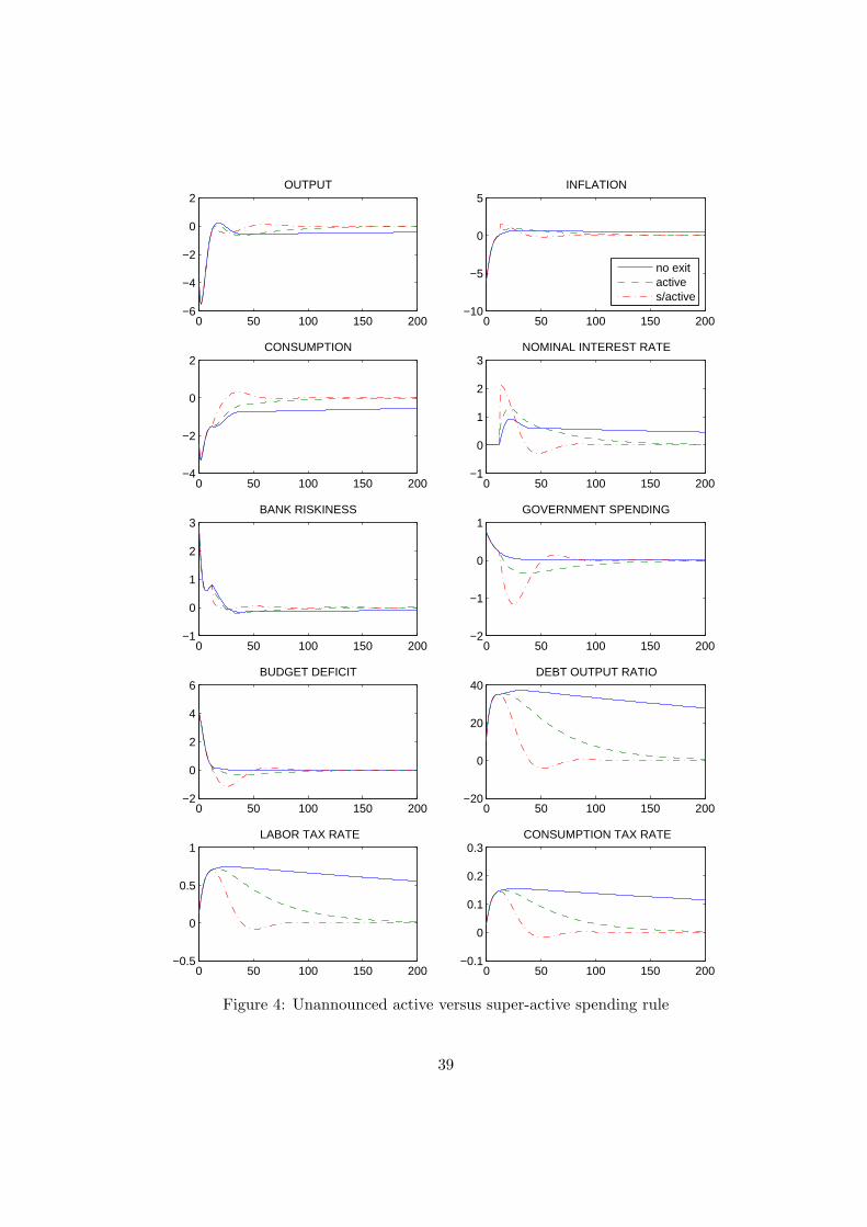
0 50 100 150 200−6

−4

−2

0

2OUTPUT

0 50 100 150 200−10

−5

0

5INFLATION

no exitactives/active

0 50 100 150 200−4

−2

0

2CONSUMPTION

0 50 100 150 200−1

0

1

2

3NOMINAL INTEREST RATE

0 50 100 150 200−1

0

1

2

3BANK RISKINESS

0 50 100 150 200−2

−1

0

1GOVERNMENT SPENDING

0 50 100 150 200−2

0

2

4

6BUDGET DEFICIT

0 50 100 150 200−20

0

20

40DEBT OUTPUT RATIO

0 50 100 150 200−0.5

0

0.5

1LABOR TAX RATE

0 50 100 150 200−0.1

0

0.1

0.2

0.3CONSUMPTION TAX RATE

Figure 4: Unannounced active versus super-active spending rule

39

0 10 20 30−6

−4

−2

0

2OUTPUT

0 10 20 30−10

−5

0

5INFLATION

no exittaxspending

0 10 20 30−4

−2

0

2CONSUMPTION

0 10 20 300

5

10NOMINAL INTEREST RATE

0 10 20 30−2

0

2

4BANK RISKINESS

0 10 20 30−2

−1

0

1GOVERNMENT SPENDING

0 10 20 30−5

0

5BUDGET DEFICIT

0 10 20 300

10

20

30

40DEBT OUTPUT RATIO

0 10 20 300

2

4

6LABOR TAX RATE

0 10 20 300

0.5

1

1.5CONSUMPTION TAX RATE

Figure 5: Tax-based versus spending-based strategy, both unannounced and super-active

40

0 50 100 150 200−6

−4

−2

0

2OUTPUT

0 50 100 150 200−10

−5

0

5INFLATION

no exittaxspending

0 50 100 150 200−4

−2

0

2CONSUMPTION

0 50 100 150 200−5

0

5

10NOMINAL INTEREST RATE

0 50 100 150 200−2

0

2

4BANK RISKINESS

0 50 100 150 200−2

−1

0

1GOVERNMENT SPENDING

0 50 100 150 200−5

0

5BUDGET DEFICIT

0 50 100 150 200−20

0

20

40DEBT OUTPUT RATIO

0 50 100 150 200−2

0

2

4

6LABOR TAX RATE

0 50 100 150 200−0.5

0

0.5

1

1.5CONSUMPTION TAX RATE

Figure 6: Tax-based versus spending-based strategy, both unannounced and super-active

41

0 10 20 30−6

−4

−2

0

2OUTPUT

0 10 20 30−10

−5

0

5

10INFLATION

tax mixconsumption taxlabor tax

0 10 20 30−4

−3

−2

−1

0CONSUMPTION

0 10 20 300

5

10NOMINAL INTEREST RATE

0 10 20 30−4

−2

0

2

4BANK RISKINESS

0 10 20 300

0.2

0.4

0.6

0.8GOVERNMENT SPENDING

0 10 20 30−10

−5

0

5BUDGET DEFICIT

0 10 20 300

10

20

30

40DEBT OUTPUT RATIO

0 10 20 300

2

4

6

8LABOR TAX RATE

0 10 20 300

1

2

3

4CONSUMPTION TAX RATE

Figure 7: Mix-tax strategy versus tax strategies tilted towards labor and consumption taxes – allin super-active, unannounced mode

42

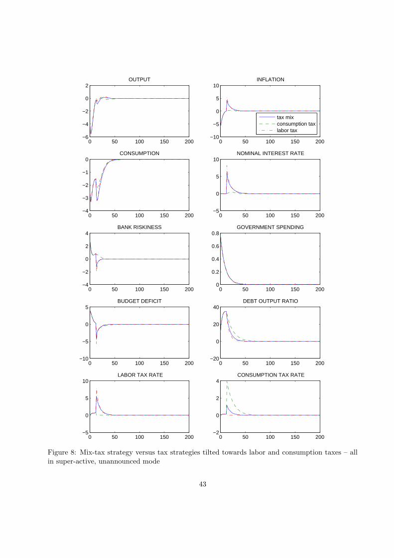
0 50 100 150 200−6

−4

−2

0

2OUTPUT

0 50 100 150 200−10

−5

0

5

10INFLATION

tax mixconsumption taxlabor tax

0 50 100 150 200−4

−3

−2

−1

0CONSUMPTION

0 50 100 150 200−5

0

5

10NOMINAL INTEREST RATE

0 50 100 150 200−4

−2

0

2

4BANK RISKINESS

0 50 100 150 2000

0.2

0.4

0.6

0.8GOVERNMENT SPENDING

0 50 100 150 200−10

−5

0

5BUDGET DEFICIT

0 50 100 150 200−20

0

20

40DEBT OUTPUT RATIO

0 50 100 150 200−5

0

5

10LABOR TAX RATE

0 50 100 150 200−2

0

2

4CONSUMPTION TAX RATE

Figure 8: Mix-tax strategy versus tax strategies tilted towards labor and consumption taxes – allin super-active, unannounced mode

43

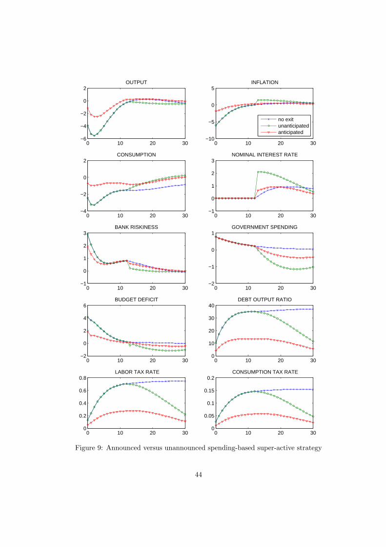
0 10 20 30−6

−4

−2

0

2OUTPUT

0 10 20 30−10

−5

0

5INFLATION

no exitunanticipatedanticipated

0 10 20 30−4

−2

0

2CONSUMPTION

0 10 20 30−1

0

1

2

3NOMINAL INTEREST RATE

0 10 20 30−1

0

1

2

3BANK RISKINESS

0 10 20 30−2

−1

0

1GOVERNMENT SPENDING

0 10 20 30−2

0

2

4

6BUDGET DEFICIT

0 10 20 300

10

20

30

40DEBT OUTPUT RATIO

0 10 20 300

0.2

0.4

0.6

0.8LABOR TAX RATE

0 10 20 300

0.05

0.1

0.15

0.2CONSUMPTION TAX RATE

Figure 9: Announced versus unannounced spending-based super-active strategy

44

0 50 100 150 200−6

−4

−2

0

2OUTPUT

0 50 100 150 200−10

−5

0

5INFLATION

no exitunanticipatedanticipated

0 50 100 150 200−4

−2

0

2CONSUMPTION

0 50 100 150 200−1

0

1

2

3NOMINAL INTEREST RATE

0 50 100 150 200−1

0

1

2

3BANK RISKINESS

0 50 100 150 200−2

−1

0

1GOVERNMENT SPENDING

0 50 100 150 200−2

0

2

4

6BUDGET DEFICIT

0 50 100 150 200−20

0

20

40DEBT OUTPUT RATIO

0 50 100 150 200−0.5

0

0.5

1LABOR TAX RATE

0 50 100 150 200−0.1

0

0.1

0.2

0.3CONSUMPTION TAX RATE

Figure 10: Announced versus unannounced spending-based super-active strategy

45

0 10 20 30−3

−2

−1

0

1OUTPUT

0 10 20 30−3

−2

−1

0

1INFLATION

fiscal leadsmoney leadsmove together

0 10 20 30−1.5

−1

−0.5

0

0.5CONSUMPTION

0 10 20 30−0.5

0

0.5

1

1.5NOMINAL INTEREST RATE

0 10 20 30−1

0

1

2BANK RISKINESS

0 10 20 30−1

−0.5

0

0.5

1GOVERNMENT SPENDING

0 10 20 30−1

0

1

2

3BUDGET DEFICIT

0 10 20 300

5

10

15

20DEBT OUTPUT RATIO

0 10 20 300

0.1

0.2

0.3

0.4LABOR TAX RATE

0 10 20 300

0.02

0.04

0.06

0.08CONSUMPTION TAX RATE

Figure 11: Sequencing and delaying

46

0 50 100 150 200−3

−2

−1

0

1OUTPUT

0 50 100 150 200−3

−2

−1

0

1INFLATION

fiscal leadsmoney leadsmove together

0 50 100 150 200−1.5

−1

−0.5

0

0.5CONSUMPTION

0 50 100 150 200−0.5

0

0.5

1

1.5NOMINAL INTEREST RATE

0 50 100 150 200−1

0

1

2BANK RISKINESS

0 50 100 150 200−1

−0.5

0

0.5

1GOVERNMENT SPENDING

0 50 100 150 200−1

0

1

2

3BUDGET DEFICIT

0 50 100 150 200−10

0

10

20DEBT OUTPUT RATIO

0 50 100 150 200−0.2

0

0.2

0.4

0.6LABOR TAX RATE

0 50 100 150 200−0.05

0

0.05

0.1

0.15CONSUMPTION TAX RATE

Figure 12: Sequencing and delaying

47

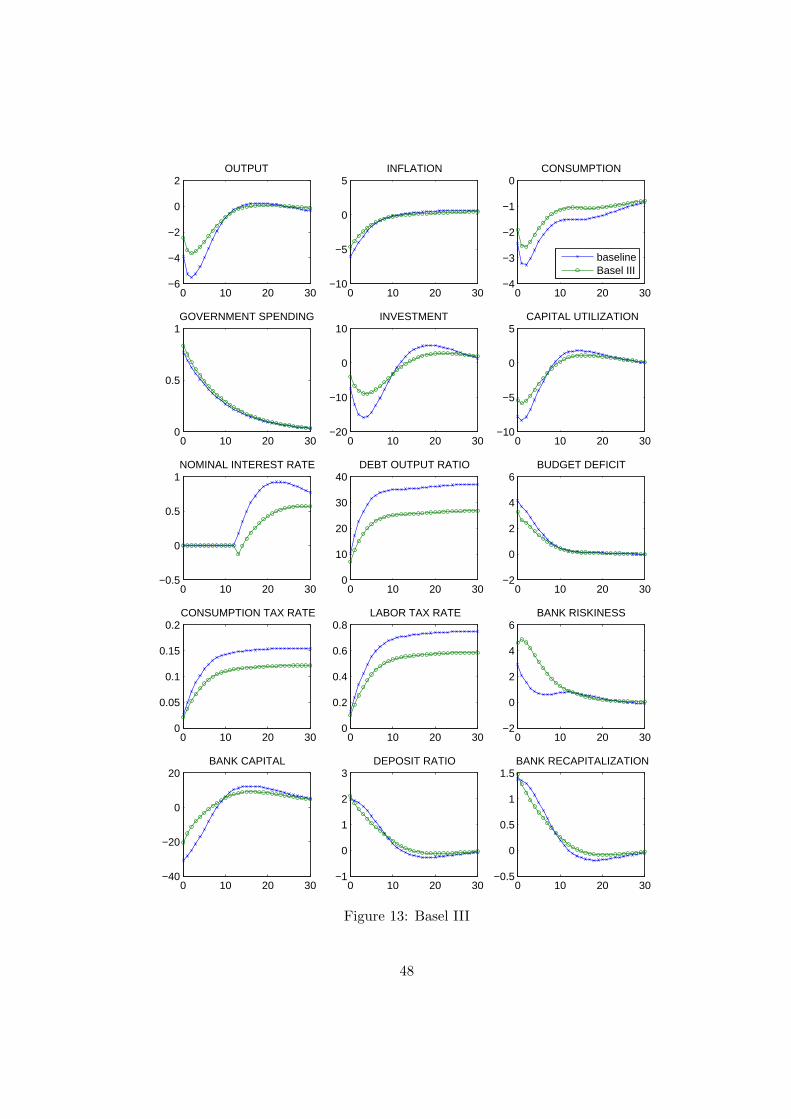
0 10 20 30−6

−4

−2

0

2OUTPUT

0 10 20 30−10

−5

0

5INFLATION

0 10 20 30−4

−3

−2

−1

0CONSUMPTION

baselineBasel III

0 10 20 300

0.5

1GOVERNMENT SPENDING

0 10 20 30−20

−10

0

10INVESTMENT

0 10 20 30−10

−5

0

5CAPITAL UTILIZATION

0 10 20 30−0.5

0

0.5

1NOMINAL INTEREST RATE

0 10 20 300

10

20

30

40DEBT OUTPUT RATIO

0 10 20 30−2

0

2

4

6BUDGET DEFICIT

0 10 20 300

0.05

0.1

0.15

0.2CONSUMPTION TAX RATE

0 10 20 300

0.2

0.4

0.6

0.8LABOR TAX RATE

0 10 20 30−2

0

2

4

6BANK RISKINESS

0 10 20 30−40

−20

0

20BANK CAPITAL

0 10 20 30−1

0

1

2

3DEPOSIT RATIO

0 10 20 30−0.5

0

0.5

1

1.5BANK RECAPITALIZATION

Figure 13: Basel III

48

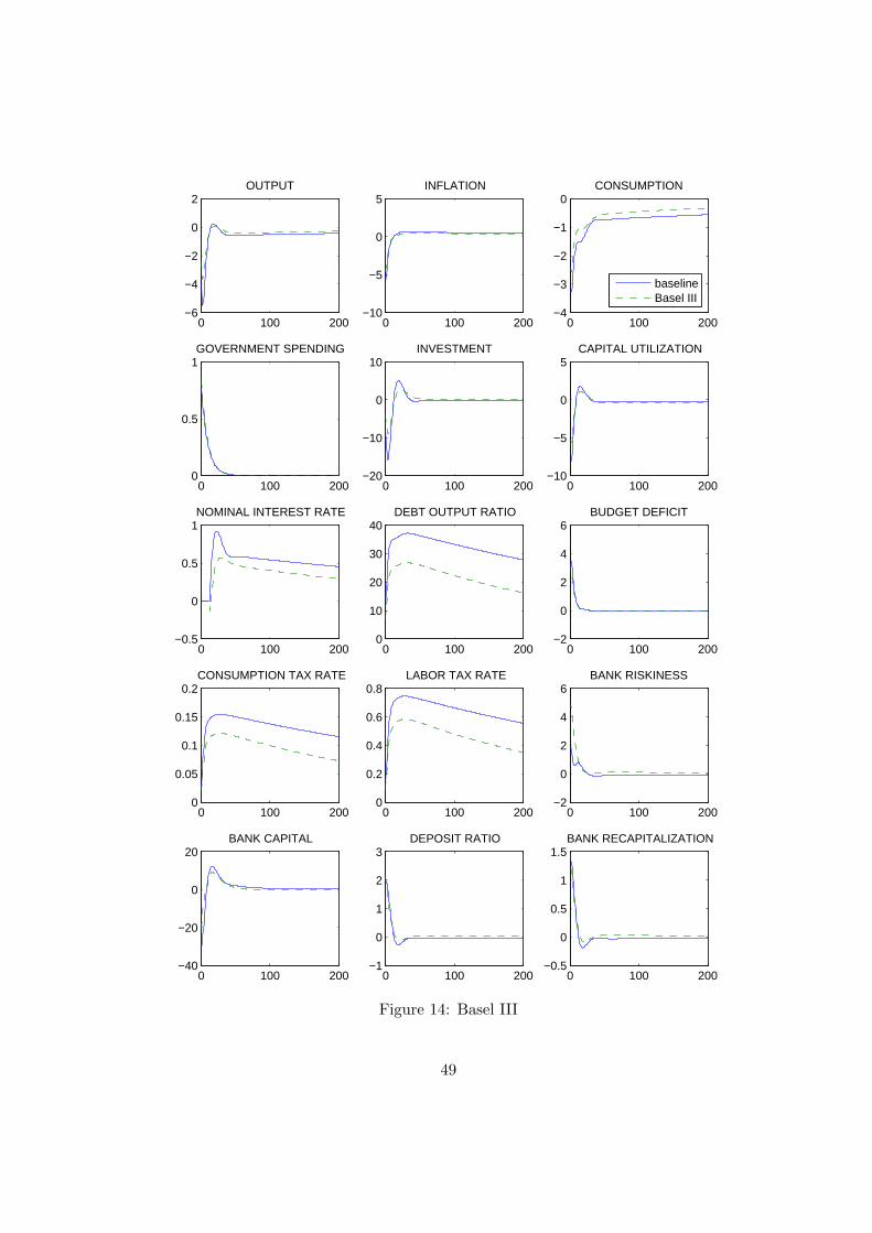
0 100 200−6

−4

−2

0

2OUTPUT

0 100 200−10

−5

0

5INFLATION

0 100 200−4

−3

−2

−1

0CONSUMPTION

baselineBasel III

0 100 2000

0.5

1GOVERNMENT SPENDING

0 100 200−20

−10

0

10INVESTMENT

0 100 200−10

−5

0

5CAPITAL UTILIZATION

0 100 200−0.5

0

0.5

1NOMINAL INTEREST RATE

0 100 2000

10

20

30

40DEBT OUTPUT RATIO

0 100 200−2

0

2

4

6BUDGET DEFICIT

0 100 2000

0.05

0.1

0.15

0.2CONSUMPTION TAX RATE

0 100 2000

0.2

0.4

0.6

0.8LABOR TAX RATE

0 100 200−2

0

2

4

6BANK RISKINESS

0 100 200−40

−20

0

20BANK CAPITAL

0 100 200−1

0

1

2

3DEPOSIT RATIO

0 100 200−0.5

0

0.5

1

1.5BANK RECAPITALIZATION

Figure 14: Basel III

49

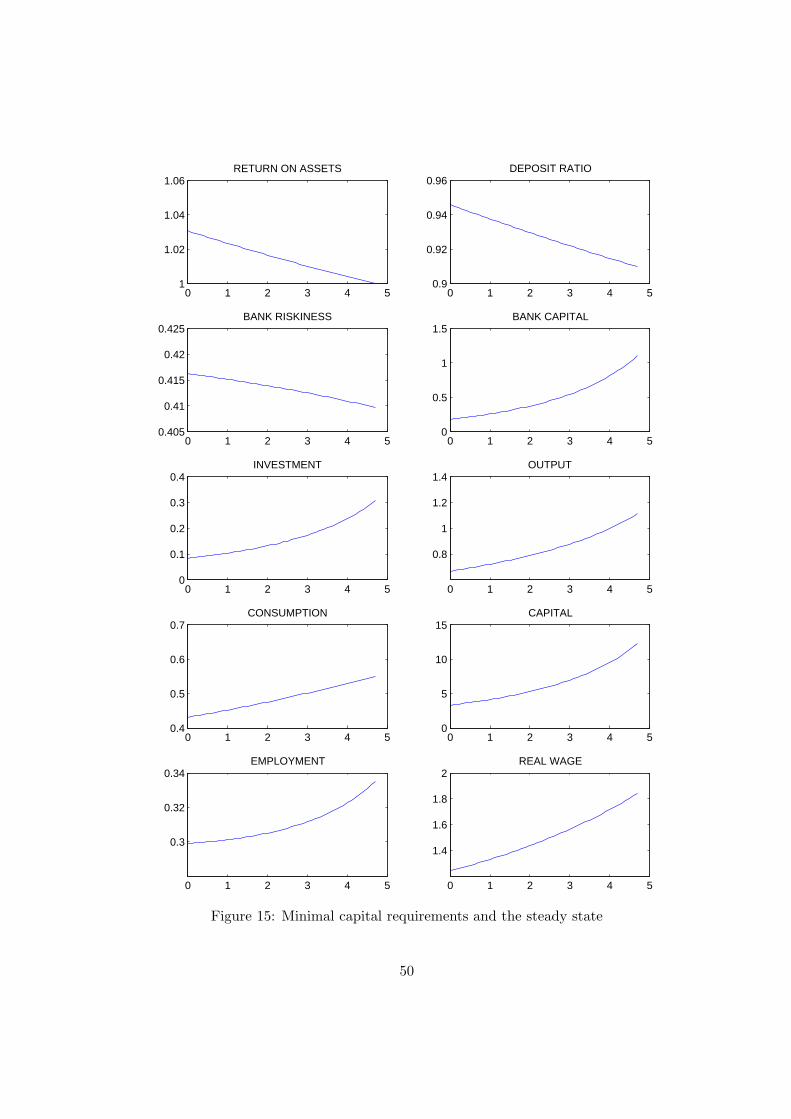
0 1 2 3 4 51

1.02

1.04

1.06RETURN ON ASSETS

0 1 2 3 4 50.9

0.92

0.94

0.96DEPOSIT RATIO

0 1 2 3 4 50.405

0.41

0.415

0.42

0.425BANK RISKINESS

0 1 2 3 4 50

0.5

1

1.5BANK CAPITAL

0 1 2 3 4 50

0.1

0.2

0.3

0.4INVESTMENT

0 1 2 3 4 5

0.8

1

1.2

1.4OUTPUT

0 1 2 3 4 50.4

0.5

0.6

0.7CONSUMPTION

0 1 2 3 4 50

5

10

15CAPITAL

0 1 2 3 4 5

0.3

0.32

0.34EMPLOYMENT

0 1 2 3 4 5

1.4

1.6

1.8

2REAL WAGE

Figure 15: Minimal capital requirements and the steady state

50

2008 2009 2010 1 2

GDP 0,3 -4,1 1,7 -5,0 -3,6

0,1 -4,9 -4,1 -5,0 -3,6

0,3 -1,1 0,6 -3,0 -2,3

-1 -11,3 -1 -12,6 -13,2

1 -1,8 -0,5 -3,4 -2,9

2,7 -0,2 1,7 -4,5 -1,6

69,6 79 84,3 82,8 91,2

2 6,2 6,3 3,5 1,7

Table 1: MATCHING THE CRISIS

Sources: OECD Econ Outlook 88, 2010 (1) Model: years after shock (2)

Periods:

GDP, % dev. from potential

Private consumption

Private investment

Employment

Consumption deflator

Public debt,% GDP

Public sector deficit, % GDP

(1) Percentage changes from previous year except when otherwise indicated. (2) Deviations from steady state

51

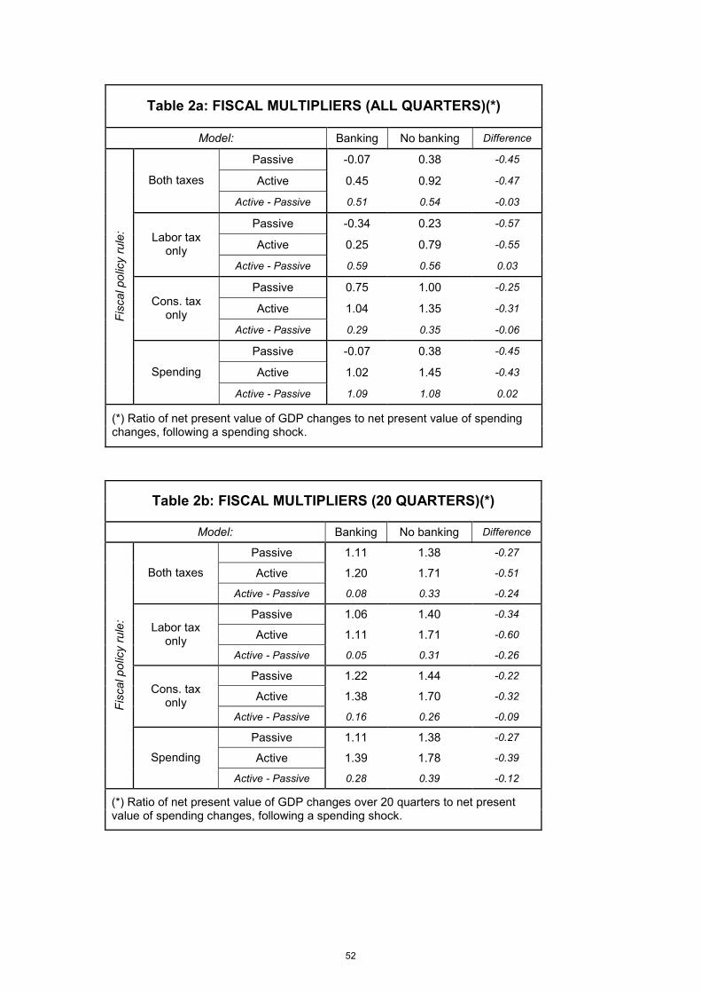
Table 2a: FISCAL MULTIPLIERS (ALL QUARTERS)(*)

Model: Banking No banking Difference

Passive -0.07 0.38 -0.45

Active 0.45 0.92 -0.47 Both taxes

Active - Passive 0.51 0.54 -0.03

Passive -0.34 0.23 -0.57

Active 0.25 0.79 -0.55 Labor tax

only

Active - Passive 0.59 0.56 0.03

Passive 0.75 1.00 -0.25

Active 1.04 1.35 -0.31 Cons. tax

only

Active - Passive 0.29 0.35 -0.06

Passive -0.07 0.38 -0.45

Active 1.02 1.45 -0.43

Fiscal policy rule:

Spending

Active - Passive 1.09 1.08 0.02

(*) Ratio of net present value of GDP changes to net present value of spending changes, following a spending shock.

Table 2b: FISCAL MULTIPLIERS (20 QUARTERS)(*)

Model: Banking No banking Difference

Passive 1.11 1.38 -0.27

Active 1.20 1.71 -0.51 Both taxes

Active - Passive 0.08 0.33 -0.24

Passive 1.06 1.40 -0.34

Active 1.11 1.71 -0.60 Labor tax

only

Active - Passive 0.05 0.31 -0.26

Passive 1.22 1.44 -0.22

Active 1.38 1.70 -0.32 Cons. tax

only

Active - Passive 0.16 0.26 -0.09

Passive 1.11 1.38 -0.27

Active 1.39 1.78 -0.39

Fiscal policy rule:

Spending

Active - Passive 0.28 0.39 -0.12

(*) Ratio of net present value of GDP changes over 20 quarters to net present value of spending changes, following a spending shock.

52

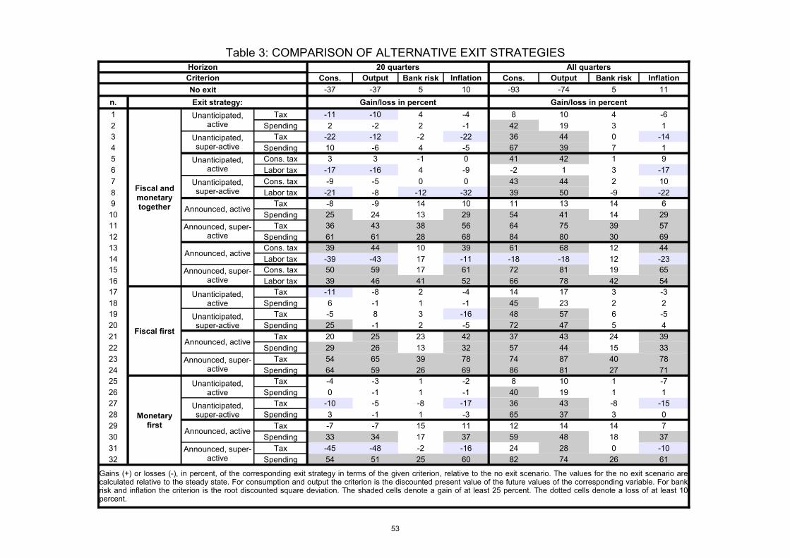
Output Inflation Output Inflation

-37 -37 5 10 -93 -74 5 11

n.

1 -11 -10 4 -4 8 10 4 -6

2 2 -2 2 -1 42 19 3 1

3 -22 -12 -2 -22 36 44 0 -14

4 10 -6 4 -5 67 39 7 1

5 3 3 -1 0 41 42 1 9

6 -17 -16 4 -9 -2 1 3 -17

7 -9 -5 0 0 43 44 2 10

8 -21 -8 -12 -32 39 50 -9 -22

9 -8 -9 14 10 11 13 14 6

10 25 24 13 29 54 41 14 29

11 36 43 38 56 64 75 39 57

12 61 61 28 68 84 80 30 69

13 39 44 10 39 61 68 12 44

14 -39 -43 17 -11 -18 -18 12 -23

15 50 59 17 61 72 81 19 65

16 39 46 41 52 66 78 42 54

17 -11 -8 2 -4 14 17 3 -3

18 6 -1 1 -1 45 23 2 2

19 -5 8 3 -16 48 57 6 -5

20 25 -1 2 -5 72 47 5 4

21 20 25 23 42 37 43 24 39

22 29 26 13 32 57 44 15 33

23 54 65 39 78 74 87 40 78

24 64 59 26 69 86 81 27 71

25 -4 -3 1 -2 8 10 1 -7

26 0 -1 1 -1 40 19 1 1

27 -10 -5 -8 -17 36 43 -8 -15

28 3 -1 1 -3 65 37 3 0

29 -7 -7 15 11 12 14 14 7

30 33 34 17 37 59 48 18 37

31 -45 -48 -2 -16 24 28 0 -10

32 54 51 25 60 82 74 26 61

Table 3: COMPARISON OF ALTERNATIVE EXIT STRATEGIESHorizon 20 quarters All quarters

Criterion Cons. Bank risk Cons. Bank risk

No exit

Exit strategy: Gain/loss in percent Gain/loss in percent

Fiscal and monetary together

Unanticipated, active

Tax

Spending

Unanticipated, super-active

Tax

Spending

Unanticipated, active

Cons. tax

Labor tax

Unanticipated, super-active

Cons. tax

Labor tax

Announced, activeTax

Spending

Announced, super-active

Tax

Spending

Announced, activeCons. tax

Labor tax

Announced, super-active

Cons. tax

Labor tax

Fiscal first

Unanticipated, active

Tax

Spending

Unanticipated, super-active

Tax

Spending

Announced, activeTax

Spending

Announced, super-active

Tax

Spending

Monetary first

Unanticipated, active

Tax

Spending

Unanticipated, super-active

Tax

Spending

Announced, activeTax

Spending

Announced, super-active

Tax

Spending

Gains (+) or losses (-), in percent, of the corresponding exit strategy in terms of the given criterion, relative to the no exit scenario. The values for the no exit scenario are calculated relative to the steady state. For consumption and output the criterion is the discounted present value of the future values of the corresponding variable. For bank risk and inflation the criterion is the root discounted square deviation. The shaded cells denote a gain of at least 25 percent. The dotted cells denote a loss of at least 10 percent.

53